Critical excitation-inhibition balance in dense neural networks
Abstract
The “edge of chaos” phase transition in artificial neural networks is of renewed interest in light of recent evidence for criticality in brain dynamics. Statistical mechanics traditionally studied this transition with connectivity as the control parameter and an exactly balanced excitation-inhibition ratio. While critical connectivity has been found to be low in these model systems, typically around , which is unrealistic for natural neural systems, a recent study utilizing the excitation-inhibition ratio as the control parameter found a new, nearly degree independent, critical point when connectivity is large. However, the new phase transition is accompanied by an unnaturally high level of activity in the network.
Here we study random neural networks with the additional properties of (i) a high clustering coefficient and (ii) neurons that are solely either excitatory or inhibitory, a prominent property of natural neurons. As a result we observe an additional critical point for networks with large connectivity, regardless of degree distribution, which exhibits low activity levels that compare well with neuronal brain networks.
Between the ordered and chaotic regimes of threshold neural networks lies the “edge of chaos,” a critical point where the length and size distributions of activity avalanches are governed by characteristic power laws. This dynamical phase transition has been thoroughly studied in random neural networks Kürten 1988; Bornholdt and Rohlf 2002; Szejka et al. 2008; Rohlf 2008, non symmetric spin glasses Derrida 1987, and random Boolean networks Derrida and Pomeau 1986; Kürten 1988; Aldana et al. 2003; Drossel 2008; Bornholdt and Kauffman 2019. Traditionally, threshold neural networks have been studied with precisely balanced excitation and inhibition, usually by randomly assigning activating and inhibiting links with equal probabilities. In these networks, criticality occurs for small average degrees Kürten 1988. However, when allowing the fraction of excitatory links as a second control parameter of the phase transition, it was recently discovered that there exist two critical lines in the --plane: one almost parallel to the axis at low and one almost independent of at some Pinheiro Neto et al. 2017, see Fig. 1.
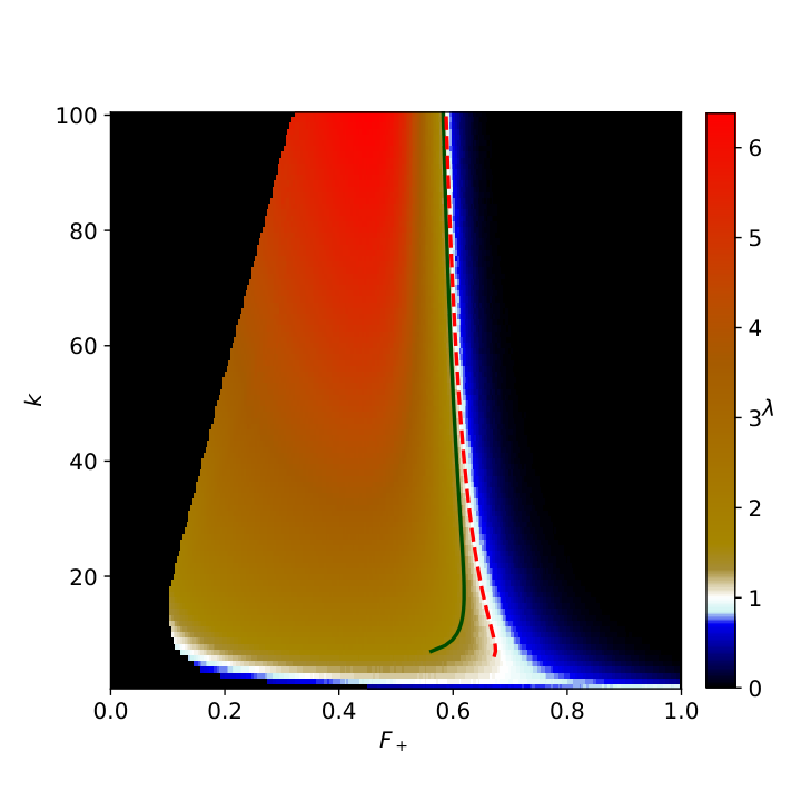
The relevance of this new critical point becomes apparent in the context of neural brain networks which exhibit a high average degree ( in human brains Huttenlocher 1979) and a characteristic imbalance between excitation and inhibition (20–30 % of neurons are inhibitory in monkey brains Hendry et al. 1987). There is a large amount of evidence suggesting that the brain operates near a critical point, namely avalanche sizes and durations governed by power laws Beggs and Plenz 2003; Friedman et al. 2012; Priesemann et al. 2014; Timme et al. 2016; Yaghoubi et al. 2018; Fontenele et al. 2019, the possibility of tuning from a subcritical regime through the critical point to a supercritical regime Haldeman and Beggs 2005, mathematical relations between critical exponents, and collapsable avalanche shapes Friedman et al. 2012; Shaukat and Thivierge 2016; Fontenele et al. 2019. Further, Fraiman et al. showed striking similarities between correlation networks extracted from brains and the Ising model at the critical point Fraiman et al. 2009. The interest in the role of criticality in the brain is illustrated by the large amount of research devoted to criticality in network models inspired by biological networks Gross and Blasius 2008; Li et al. 2017; Clawson et al. 2017; Brochini et al. 2016; Gautam et al. 2015; Shriki and Yellin 2016; Rodriguez et al. 2017; Ferraz et al. 2017.
Unfortunately, the high-degree critical point of Fig. 1 exists in a high-activity regime which is unrealistic for brain networks. We find, however, an additional critical point that persists at low activities, at the left flank of the high sensitivity region, when including additional network properties characteristic of brain networks, thereby providing a more likely network model candidate for describing the processes behind brain criticality.
We use threshold networks consisting of nodes connected by directed edges, whose node states are updated in parallel according to
| (1) |
where is the node ’s state at time and is the weight of the connection from node to node .
The weights can be if there is no connection between nodes and , or otherwise.
The weights of existing connections are chosen randomly with excitatory links chosen with probability .
Initial states of the nodes are chosen according to a random initial activity .
A simple quantity that we use to measure criticality is the sensitivity Luque and Solé 1997; Shmulevich and Kauffman 2004.
Imagine switching one node’s state in the current time step; then is defined as the average number of nodes
whose states will then be different in the next time step from what they would have been otherwise.
If sensitivity is smaller or larger than 1, perturbations will quickly die out or dominate the entire network, respectively.
Hence, at , the network is in a critical state.
First, in order to establish whether the vertical white line defined by seen in Fig. 1
indeed is a critical point, we measure the averages of multiple quantities of interest, as well as
the average sensitivity for time steps after letting the network relax from its initial condition
within time steps (tests show that increasing this time or waiting until an attractor is reached — where possible,
attractors cannot be found in a reasonable amount of time for — does not change the results)
for different values of . Afterwards, we can plot the measured quantities as a function of sensitivity.
The measured quantities are the network’s activity , the fraction of nodes which do not change their state
within the time steps , and the average number of state changes per node and time step .
This measurement is shown in Fig. 2.
For , essentially all nodes are static
(i.e. remaining in one state, either active or inactive)
and almost no flips happen, whereas for the number
of static nodes drops and the number of flips increases, so is a boundary between order and chaos.
Also note that the network’s activity is very high at the critical point. It seems, therefore, that this critical
point cannot underlie a mechanism that defines criticality in the brain, as almost all neurons constantly firing is not realistic.
Further, we measure avalanche sizes and durations at the critical point, as described in the Supplemental Material
Sup; see Fig. 3.
Also, (b) attractor and (d) transient length distributions for networks with , , , , and . The slopes shown in red are (b) and (d) . Logarithmic binning is used for all four figures.
We observe power laws in both avalanche size and duration distributions.
Finally, we measure the attractor and transient lengths, as well as the average sensitivity
within the attractor for a number of different network realizations for fixed parameters.
We only use parameter and attractor lengths of networks whose average sensitivity
is within with .
Attractor and transient length distributions are shown in FIG. 3.
Both the attractor lengths as well as the right flank of the transient length distributions
show clear power laws, as is to be expected for critical networks Bhattacharjya and Liang 1996.
All of the above discussed properties lead us to conclude that this is indeed a critical point.
We use Derrida’s annealed approximation Derrida and Pomeau 1986,
adopted for threshold networks Bornholdt and Rohlf 2002,
to estimate the critical as a function of , and arrive at the equation
| (2) |
Under the assumption of large average degree , , this can be simplified to
| (3) |
See Supplemental Material Sup for details. Figure 1 shows a comparison of Eq. (3), as well as the numerical solution of Eq. (2), with our simulation results.
Let us now focus on the the left flank of the central high sensitivity region in Fig. 1. When lowering the value of from intermediate values towards , sensitivity seems to suddenly drop to from values larger than . In the simulations this is due to a sudden drop in persistent activity: All activity dies out before the average sensitivity crosses through one. Critical sensitivity here falls into the left (black) region of entirely inactive networks whose sensitivity is not shown (as only persisting activity is relevant and, therefore, plotted).
However, as a central observation of our study, we find that networks
can be kept from abruptly dying out for low by introducing
two properties to the network: increasing the networks’ clustering
coefficient and requiring that nodes have either only excitatory
or only inhibitory outgoing edges (Dale’s principle). Both of these
properties are prominent features of brain networks
Stephan et al. 2000; Sporns and Zwi 2004; Sporns et al. 2007; Bassett and Bullmore 2006; Dale 1935.
Note that these properties do not necessarily cause networks to show
finite activity for values of in which the random network has
zero activity but instead that the activity goes continuously
towards zero with lowering instead of abruptly dropping to zero.
We believe the mechanism underlying the left flank’s survival to be as follows:
If two excitatory nodes which are connected to each other are active,
then for high clustering coefficients, they are likely to have shared neighbors
and can therefore combine their efforts to also activate these neighbors
more easily than in random networks and thereby create islands of surviving activity.
The contribution of nodes being either excitatory or inhibitory
is likely that if few random nodes are active within a region,
this property significantly increases the variance of the
relative number of activating signals in that region
and therefore increases the probability of areas exhibiting
high excitation by random chance.
We also see that the sensitivity in clustered graphs with nodes either fully excitatory or inhibitory closely follows the sensitivity of random graphs for high values of but then drops off for lower , see Fig. 4.
This is likely due to nodes in the center of activity islands receiving
many more excitatory connections than necessary for activation.
This both lowers the overall activity because these redundant excitatory
signals essentially lower the network’s total excitation and lower
the sensitivity because only nodes with an input sum near the
excitation threshold contribute to it.
Networks with only a high clustering coefficient, without the second property of nodes having either only excitatory or only inhibitory outgoing edges, can also show surviving activity on the left flank for some initial configurations and for exceedingly high clustering coefficients and thresholds, but even then the left flank drops sharply towards zero. In the following, let us denote networks obeying Dale’s principle Dale 1935, i.e. networks consisting of excitatory neurons and inhibitory neurons as EIN networks, as opposed to networks with excitatory/inhibitory edges which we will call EIE networks.
Since the network’s activity does not abruptly die out on the left flank anymore for clustered EIN networks, a second critical point can be found here, as shown in Fig. 5 and Fig. 4 (a).

Plotting the sensitivity in the --plane in Fig. 5, we now see that the left flank indeed exhibits critical sensitivity (white color). Note that, in contrast to the first critical point at the right flank of the sensitive region, this second critical point at the left flank exists in a low-activity state, making it more interesting for real life applications, such as studying mechanisms underlying brain criticality.
To construct networks with different high clustering coefficients, we here use directed Watts-Strogatz (WS) networks Watts and Strogatz 1998; Song and Wang 2014b. The original WS model consists of a ring of neurons with periodic boundary conditions in which every neuron is connected to its nearest neighbors. Then, connections are randomly rewired with rewiring probability . We use an essentially equivalent implementation without explicit rewiring from Song and Wang 2014b in which the probability of a connection from a node to a node existing is
| (4) |
where and is the distance between nodes and on the ring, i.e. . The third term has been added to enable uneven values of . By manipulating the rewiring probability , we can vary a network’s clustering coefficient and average path length. The Watts-Strogatz model’s strength is that when varying , there is a region in which the clustering coefficient is nearly constant while the average path length changes drastically and a second region in which the clustering coefficient changes and the average path length is nearly constant, enabling us to isolate these two parameters’ effects.
In our study of clustered EIN networks, we find that the second critical point comes into existence in the region in which the clustering coefficient changes, while it is unaffected by changes within the region in which the clustering coefficient is constant. Therefore, a high clustering coefficient is sufficient to enable the second critical point’s existence.
The influence of thresholds and clustering coefficients, as well as the difference between EIE and EIN networks is shown in Figs. 4 (b) and 6.

So far, our networks had degree distributions centered around an average value; however,
random or Watts-Strogatz models rarely describe real-life networks.
Scale-free or similar networks with a broad degree distribution are significantly more abundant in nature.
In fact, for neuronal networks, cumulative degree distributions ranging from power laws
Varshney et al. 2011; van den Heuvel et al. 2008; Eguíluz et al. 2005 over exponentially truncated power laws
Hayasaka and Laurienti 2010; He et al. 2007; Iturria-Medina et al. 2008; Achard et al. 2006; Gong et al. 2009 to exponential laws Modha and Singh 2010; Amaral et al. 2000; Hagmann et al. 2008; de Santos-Sierra et al. 2014 have been found, with the observation that
distributions following exponentially truncated power laws increasingly resemble true power laws
for measurements on finer scales Hayasaka and Laurienti 2010.
In analogy to the brain, we focus on EIN networks with a broad link distribution.
For generating the topology, we
require an algorithm that (1) can produce a scale-free graph in which low-degree nodes can exist, (2) can initialize large networks fast, (3) can produce networks with variable clustering coefficient, as we have already seen that this can have a large impact on criticality, and if possible (4) can also produce other degree distributions similar to scale-free graphs.
For this purpose, we adapt the algorithm described by Lo et al. Lo et al. 2012,
a particularly efficient implementation of preferential attachment Barabási and Albert 1999,
to fit our criteria.
In our algorithm, we start with a single node and iteratively add a connection between two nodes every two time steps, so that the sum of in and out degrees in the network increases by one per time step.
The origins and targets of these added nodes are chosen by preferential attachment, meaning that the probability of a node being chosen is proportional to the sum of its in and out degree plus an offset , which ensures that the probability of previously unconnected nodes receiving connections is nonzero.
Further, every time steps, a new node is added to the network.
One significant difference between our algorithm and other algorithms creating scale-free graphs is that the newly added edges need not connect to the newly added node, but can instead connect any two nodes in the system, allowing low-degree nodes to exist in the final network.
This process is repeated multiple times and the connections of every initialization are added together into one network until the desired average degree is reached.
Finally, we add random incoming and outgoing connections to every node, where is the first integer with , so that all nodes have the chance of being activated.
For a detailed description of this algorithm, see the Supplemental Material Sup.
The two parameters and control whether the resulting degree distribution is scale free or an exponentially truncated power law and also the clustering coefficient.
In general, lower and higher lead to scale-free distributions with high clustering, whereas high and low lead to low clustering truncated power law distributions.
Studying the dynamics of EIN networks with such a topology, we find that for scale-free graphs the right critical point still exists (see Fig. 7), and that the sensitivity splits into two paths on the right flank and is therefore no longer solely dependent on . The two different paths are dependent on whether the network’s largest node is excitatory or inhibitory (in our algorithm, there is a clear hierarchy between nodes, dictated by when they were introduced to the network, and therefore the first node is always clearly larger than the rest, so no multiple nodes are competing for the spot of largest node). Similarly to the existence of the left flank in WS networks, this split in the sensitivity is amplified by high clustering coefficients and thresholds.
Figure 7 also shows the existence of the left flank’s second critical point for high clustering coefficients and thresholds ; see Fig. 7. For low clustering coefficients, the left flank still dies out. High clustering coefficients and thresholds lower the sensitivity curve’s slope, so that for certain parameters the sensitivity, and therefore criticality, is almost constant over a wide area of ; see Fig. 7 (b).
To summarize, in threshold neural networks, a phase transition between
a chaotic and a quiescent regime has been found for highly clustered networks
with exclusively excitatory-inhibitory nodes.
This critical point exhibits a persisting, yet low level of average activity
(which in unclustered networks would die out).
Besides the requirement of a certain level of clustering, it is robust both
for random as well as broad (scale-free) degree distributions.
This new critical point is of particular interest to neuroscience because
it is relatively independent of the degree
and may, therefore, occur at the large average degree present in brains.
Furthermore, the main prerequisites for this critical point’s existence are present in the brain:
a highly clustered architecture and nodes being either exclusively excitatory or inhibitory (Dale’s principle).
It can only be speculated what role criticality may play in nature.
It has been discussed that it could optimize a network’s information processing capabilities.
Yet also, dynamical phase transitions are a simple means that physics provides, allowing
a complex system to tune to an intermediate activity regime with great ease.
Last but not least, research has shown that the balance between excitation and inhibition in the brain,
which needs to be a specific value for a network to be critical in our model, is vital for a functioning brain
Haider et al. 2006; Rubenstein and Merzenich 2003; Davenport et al. 2019; Antoine et al. 2019; Murray and Wang 2018
and that disturbing this balance can negatively impact information processing Yizhar et al. 2011.
Interestingly, the ratio of excitatory and inhibitory neurons in brain networks
is observed to be almost constant throughout an organism’s development,
and feedback algorithms that regulate this ratio are currently discussed Sahara et al. 2012.
This supports our hypothesis that the critical point described in this paper,
resulting from the statistical mechanics of a dynamical phase transition,
may provide a natural target value for mechanisms that regulate the
excitation-inhibition balance in the brain.
References
- Kürten (1988) K. Kürten, Phys. Lett. A 129, 157 (1988).
- Bornholdt and Rohlf (2002) S. Bornholdt and T. Rohlf, Physica A 310, 245 (2002).
- Szejka et al. (2008) A. Szejka, T. Mihaljev, and B. Drossel, New J. Phys. 10, 063009 (2008).
- Rohlf (2008) T. Rohlf, Phys. Rev. E 78, 066118 (2008).
- Derrida (1987) B. Derrida, J. Phys. A 20, L721 (1987).
- Derrida and Pomeau (1986) B. Derrida and Y. Pomeau, Europhys. Lett. 1, 45 (1986).
- Kürten (1988) K. E. Kürten, J. Phys. A 21, L615 (1988).
- Aldana et al. (2003) M. Aldana, S. Coppersmith, and L. Kadanoff, in Perspectives and Problems in Nonlinear Science, edited by E. Kaplan, J. Marsden, and K. Sreenivasan (Springer, 2003).
- Drossel (2008) B. Drossel, in Reviews of Nonlinear Dynamics and Complexity, Vol. 1, edited by H. Schuster (Wiley-VCH, Weinheim, 2008).
- Bornholdt and Kauffman (2019) S. Bornholdt and S. Kauffman, Journal of Theoretical Biology 467, 15 (2019).
- Pinheiro Neto et al. (2017) J. Pinheiro Neto, M. A. M. de Aguiar, J. A. Brum, and S. Bornholdt, arXiv e-prints , arXiv:1712.08816 (2017), arXiv:1712.08816 [nlin.AO] .
- Huttenlocher (1979) P. R. Huttenlocher, Brain Res. 163, 195 (1979).
- Hendry et al. (1987) S. Hendry, H. D. Schwark, E. Jones, and J. Yan, J. Neurosci. 7, 1503 (1987).
- Beggs and Plenz (2003) J. Beggs and D. Plenz, J. Neurosci. 23, 11167 (2003).
- Friedman et al. (2012) N. Friedman, S. Ito, B. Brinkman, M. Shimono, R. DeVille, K. Dahmen, J. Beggs, and T. Butler, Phys. Rev. Lett. 108, 208102 (2012).
- Priesemann et al. (2014) V. Priesemann, M. Wibral, M. Valderrama, R. Pröpper, M. Quyen, T. Geisel, J. Triesch, D. Nikolić, and M. Munk, Front. Syst. Neurosci. 8, 108 (2014).
- Timme et al. (2016) N. Timme, N. Marshall, N. Bennett, M. Ripp, E. Lautzenhiser, and J. Beggs, Front. Physiol. 7, 425 (2016).
- Yaghoubi et al. (2018) M. Yaghoubi, T. de Graaf, J. Orlandi, F. Girotto, M. Colicos, and J. Davidsen, Sci. Rep. 8, 3417 (2018).
- Fontenele et al. (2019) A. J. Fontenele, N. A. de Vasconcelos, T. Feliciano, L. A. A. Aguiar, C. Soares-Cunha, B. Coimbra, L. D. Porta, S. Ribeiro, A. J. Rodrigues, N. Sousa, P. V. Carelli, and M. Copelli, Phys. Rev. Lett. 122, 208101 (2019).
- Haldeman and Beggs (2005) C. Haldeman and J. Beggs, Phys. Rev. Lett. 94, 058101 (2005).
- Shaukat and Thivierge (2016) A. Shaukat and J. Thivierge, Front. Comput. Neurosci. 10, 29 (2016).
- Fraiman et al. (2009) D. Fraiman, P. Balenzuela, J. Foss, and D. Chialvo, Phys. Rev. E 79, 061922 (2009).
- Gross and Blasius (2008) T. Gross and B. Blasius, J. Royal Soc. Interface 5 20, 259 (2008).
- Li et al. (2017) X. Li, Q. Chen, and F. Xue, Phil. Trans. R. Soc. A 375, 20160286 (2017).
- Clawson et al. (2017) W. Clawson, N. Wright, R. Wessel, and W. Shew, PLoS Comput. Biol. 13, e1005574 (2017).
- Brochini et al. (2016) L. Brochini, A. de Andrade Costa, M. Abadi, A. Roque, J. Stolfi, and O. Kinouchi, Sci. Rep. 6 (2016).
- Gautam et al. (2015) S. Gautam, T. Hoang, K. McClanahan, S. Grady, and W. Shew, PLoS Comput. Biol. 11, e1004576 (2015).
- Shriki and Yellin (2016) O. Shriki and D. Yellin, PLoS Comput. Biol. 12, e1004698 (2016).
- Rodriguez et al. (2017) B. V. Rodriguez, A. Avena-Koenigsberger, O. Sporns, A. Griffa, P. Hagmann, and H. Larralde, Sci. Rep. 7, 13020 (2017).
- Ferraz et al. (2017) M. Ferraz, H. Melo-Silva, and A. Kihara, PLoS One 12, e0184367 (2017).
- Luque and Solé (1997) B. Luque and R. Solé, Phys. Rev. E 55, 257 (1997).
- Shmulevich and Kauffman (2004) I. Shmulevich and S. Kauffman, Phys. Rev. Lett. 93, 048701 (2004).
- (33) See Supplemental Material at [URL] for details on the annealed approximation and simulation methods .
- Bhattacharjya and Liang (1996) A. Bhattacharjya and S. Liang, Phys. Rev. Lett. 77, 1644 (1996).
- Stephan et al. (2000) K. E. Stephan, C.-C. Hilgetag, G. A. P. C. Burns, M. A. O’Neill, M. P. Young, and R. Kötter, Philos Trans R Soc Lond B Biol Sci. 355, 111 (2000).
- Sporns and Zwi (2004) O. Sporns and J. D. Zwi, Neuroinformatics 2, 145 (2004).
- Sporns et al. (2007) O. Sporns, C. J. Honey, and R. Kötter, PLoS One 2, e1049 (2007).
- Bassett and Bullmore (2006) D. S. Bassett and E. Bullmore, The Neuroscientist 12, 512 (2006).
- Dale (1935) H. Dale, Proceedings of the Royal Society of Medicine 28, 319 (1935), 19990108[pmid].
- Watts and Strogatz (1998) D. Watts and S. Strogatz, Nature 393, 440 (1998).
- Song and Wang (2014b) H. F. Song and X.-J. Wang, Phys. Rev. E 90, 062801 (2014b).
- Varshney et al. (2011) L. Varshney, B. Chen, E. Paniagua, D. Hall, and D. Chklovskii, PLoS Comput. Biol. 7, e1001066 (2011).
- van den Heuvel et al. (2008) M. van den Heuvel, C. Stam, M. Boersma, and H. H. Pol, Neuroimage 43, 528 (2008).
- Eguíluz et al. (2005) V. Eguíluz, D. Chialvo, G. Cecchi, M. Baliki, and A. Apkarian, Phys. Rev. Lett. 9, 018102 (2005).
- Hayasaka and Laurienti (2010) S. Hayasaka and P. Laurienti, Neuroimage 50, 499 (2010).
- He et al. (2007) Y. He, Z. Chen, and A. Evans, Cereb. Cortex 17, 2407 (2007).
- Iturria-Medina et al. (2008) Y. Iturria-Medina, R. Sotero, E. Canales-Rodríguez, Y. Alemán-Gómez, and L. Melia-Garcia, Neuroimage 40, 1064 (2008).
- Achard et al. (2006) S. Achard, R. Salvador, B. Whitcher, J. Suckling, and E. Bullmore, Neurosci. 26, 63 (2006).
- Gong et al. (2009) G. Gong, Y. He, L. Concha, C. Lebel, D. Gross, A. Evans, and C. Beaulieu, Cereb. Cortex 19, 524 (2009).
- Modha and Singh (2010) D. Modha and R. Singh, Proc. Natl. Acad. Sci. USA 107, 13485 (2010).
- Amaral et al. (2000) L. Amaral, A. Scala, M. Barthélémy, and H. Stanley, Proc. Natl. Acad. Sci. USA 97, 11149 (2000).
- Hagmann et al. (2008) P. Hagmann, L. Cammoun, X. Gagandet, R. Meuli, C. Honey, V. Wedeen, and O. Sporns, PLoS Biol. 6, e159 (2008).
- de Santos-Sierra et al. (2014) D. de Santos-Sierra, I. S. n a Nadal, I. Leyva, J. A. Almendral, S. Anava, A. Ayali, D. Papo, and S. Boccaletti, PloS One 9, e85828 (2014).
- Lo et al. (2012) Y. Lo, C. Li, and S. Lin, International Conference on Privacy, Security, Risk and Trust and International Conference on Social Computing, SocialCom-PASSAT 28, 229 (2012) (IEEE, Piscataway Township NJ).
- Barabási and Albert (1999) A. Barabási and R. Albert, Science 286, 509 (1999).
- Haider et al. (2006) B. Haider, A. Duque, A. R. Hasenstaub, and D. A. McCormick, J. Neurosci. 26, 4535 (2006).
- Rubenstein and Merzenich (2003) J. L. R. Rubenstein and M. M. Merzenich, Genes Brain Behav. 2, 255 (2003).
- Davenport et al. (2019) E. C. Davenport, B. R. Szulc, J. Drew, J. Taylor, T. Morgan, N. F. Higgs, G. López-Doménech, and J. T. Kittler, Cell Rep. 26, 2037 (2019).
- Antoine et al. (2019) M. W. Antoine, T. Langberg, P. Schnepel, and D. E. Feldman, Neuron 101, 648 (2019).
- Murray and Wang (2018) J. D. Murray and X.-J. Wang, in Computational Psychiatry, edited by A. Anticevic and J. D. Murray (Academic Press, 2018) pp. 3 – 25.
- Yizhar et al. (2011) O. Yizhar, L. E. Fenno, M. Prigge, F. Schneider, T. J. Davidson, D. J. O’Shea, V. S. Sohal, I. Goshen, J. Finkelstein, J. T. Paz, K. Stehfest, R. Fudim, C. Ramakrishnan, J. R. Huguenard, P. Hegemann, and K. Deisseroth, Nature 477, 171 (2011).
- Sahara et al. (2012) S. Sahara, Y. Yanagawa, D. D. M. O’Leary, and C. F. Stevens, J. Neurosci. 32, 4755 (2012).