The Power Light Cone of the Discrete Bak-Sneppen, Contact and other local processes

There are different ways of defining the DBS process. These definitions map to each other in straightforward ways, and only slightly differ in the notion of a “time step”. For example, one can define a time step as picking a random vertex (not necessarily with value $0$) and then not do anything when it has value $1$ but still count it as a time step. To study the process for an infinite-sized system, one can consider a continuous-time version of this process with exponential clocks at every vertex. Resampling of a vertex and its neighbors happens when the clock of the vertex rings and the current value of the vertex is zero.

In this section we consider the discrete-time process on a finite system, where a $0$-vertex is picked in every time step, and the process terminates when an all-$1$ state is reached. Furthermore, we will always refer to the vertex-state $0$ as active and $1$ as inactive.

From numerical simulations it is apparent that there is a phase transition in the DBS process when $p$ goes from 0 to 1. There is some critical probability $p_{c}$ such that for $p<p_{c}$ the active vertices quickly die out and the system is pushed toward a state with no active vertices. However for $p>p_{c}$, the active vertices have the overhand and dominate the system. This phase transition can clearly be seen in Figure 1 from two different perspectives: (a) We have computed the expected number of steps per vertex, on a cycle of length $n$, to reach the all-inactive state, where the vertices are initialized i.i.d. to active with probability $p$. (b) We have computed the probability that the end of a (non-periodic) chain is activated when the process is started with only one active vertex on the other end.

Let us write these functions as a power-series in $p$ and in $q=1-p$ respectively.

We will define these functions in more detail in Section 3, where we show, amongst other things, that they are rational functions for each $n$. For example

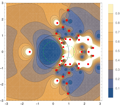
Although they only have an operational meaning for $p\in[0,1]$, we give a plot of such a function over the complex plane, see Figure 2. The plot shows the poles of $S_{(6)}(p)$, which seem to approach the value $p_{c}$ on the real line (for larger $n$ see Figure 5). Something similar happens for partition functions in statistical physics. The partition function is usually in the denominator of observable physical quantities, so that its zeroes are the poles of such quantities. A classic result on the partition function for certain gasses [YL52] shows that when an open region around the real axis is free of zeroes, then many physical quantities are analytic in that region and therefore there is no phase transition. In [PR18] the hardcore model on graphs with bounded degree is studied, and it is proven that the partition function has zeroes in the complex plane arbitrary close to the critical point.

For now, we simply want to highlight the behaviour of the coefficients $a^{(n)}_{k}$ and $b^{[n]}_{k}$. Table 1 and Table 2 show numerical values of the coefficients $a^{(n)}_{k}$ and $b^{[n]}_{k}$ respectively.⁴⁴ 4 At first sight one is tempted to conjecture that the coefficients $a^{(n)}_{k}$ are all non-negative and are monotone increasing with $n$. Unfortunately neither of these conjectures hold since $a^{(10)}_{1114}<0$. We found this counterexample by observing that the radius of convergence for $R_{10}(p)$ is less than $0.96$, which considering that $R_{10}(p)$ is bounded on $[0,0.96]$ implies that there must be a negative coefficient in its power series.

A quick look at the table immediately reveals the stabilization of coefficients:

We now know the first few terms of the power series for arbitrary large systems and we can proceed to use methods of series analysis. By applying the method of Padé approximants, we can estimate $p_{c}\approx 0.6352$. More details on this can be found in Section 3.

Our proofs are based on an observation that we call the Power Light Cone. Let $X$ be a set of vertices, and let $L_{X}$ be an event that is local on $X$, meaning that the event depends only on what happens to the vertices in $X$. For example, when $X=\{v_{0}\}$ and $L_{X}$ is the event that vertex $v_{0}$ is picked at least $r$ times, then $L_{X}$ is local on $X$. In Section 2 we will give a more precise definition of local events. We now wish to compare the probability $\mathbb{P}(L_{X})$ when the process is initialized in two different starting states, $A$ and $A^{\prime}$. When $A$ and $A^{\prime}$ differ only on vertices that are at least a distance $d$ away from $X$, then we have

By the notation $\mathcal{O}(p^{d})$ we mean that when this quantity is written as power series in $p$, then the first $d-1$ terms of the series are zero. It only has non-zero terms of order $p^{d}$ and higher, i.e. the two probabilities agree on at least the first $d-1$ terms of their power series. This is the essence of the Power Light Cone. A vertex that is a distance $d$ away from the set $X$ will only influence probabilities and expectation values of $X$-local events with terms of order $p^{d}$ or higher. The intuition behind this is that the probability of a single activation is $\mathcal{O}(p)$ and in order for such a vertex to influence the state of a vertex in $X$, it needs to form a chain of activations of size $d$ to reach $X$. This observation will also allow us to compare the process on systems of different sizes.

This idea applies to expectation values as well. Consider the expected number of steps per vertex on a cycle. By translation invariance, we have

making it a $\{1\}$-local quantity. If we add an extra vertex to the cycle, the expectation value only changes by a term of order $\mathcal{O}(p^{n/2})$ since the new vertex has distance $n/2$ to vertex $1$.

Now we present the results that exhibit the power light cone. The intuition is that if two vertices have distance $d$ in the graph, then the only way they can affect each other is that an interaction chain is forming between them, meaning that every vertex gets activated at least once in between them.

When we write $f(p)=\mathcal{O}(p^{k})$ for some function $f$ then we mean the following: when $f(p)$ is written as a power-series in $p$, i.e., $f(p)=\sum_{i=0}^{\infty}\alpha_{i}p^{i}$, then $\alpha_{i}=0$ for $0\leq i\leq k-1$.

The proof goes by induction on $d(X,Y)$. For the base case, $d(X,Y)=1$, first note that when $p=0$, the process initializes everything to inactive by property (i). Depending on whether this atomic event is included in $L_{X}$, the probability $\mathbb{P}(L_{X})$ for $p=0$ (i.e. the constant term) is either 0 or 1 and independent of the graph.

Now we show the inductive step, assuming we know the statement for $d$, and that $d(X,Y)=d+1$. First we assume, that $\mathrm{RI}^{(X)}\subseteq\overline{L_{X}}$, i.e., $L_{X}\subseteq\mathrm{BA}^{(X)}$. Define

When $L_{X}^{i}$ holds, all vertices at distance $i$ remain inactive, but for all $j\leq i-1$ there exists a vertex at distance $j$ that become active. These events form a partition $L_{X}=\dot{\bigcup}_{i\in[d+1]}L_{X}^{i}$. Below we depict $L_{X}^{i}$ graphically:

It is easy to see that for all $i\in[d+1]$ we have $L_{X}^{i}\subseteq\mathrm{BA}^{(X)}\cap\bigcap_{j\in[i-1]}\mathrm{BA}^{(\overline{\partial}(X,j))}$, and therefore by Lemma 8 we get

Now we use, for all $i\in[d]$, the Splitting lemma 7 with $S=\overline{\partial}(X,i)$ to split $\Gamma(X,i-1)$ from $G\setminus\Gamma(X,i)$. We get

Therefore

We finish the proof by observing that by $\mathrm{RI}^{(X)}$ is an atomic event of the sigma algebra of the local events of $X$, so if $\mathrm{RI}^{(X)}\nsubseteq\overline{L_{X}}$, then we necessarily have $\mathrm{RI}^{(X)}\subseteq L_{X}$. Therefore we can use the above proof with $C_{X}:=\overline{L_{X}}$ and use that $\mathbb{P}(L_{X})=1-\mathbb{P}(C_{X})$. $\Box$

The proof of this lemma is analogous to the proof of Lemma 9 and can be found in Appendix A.

In order to state our general result about the stabilization of the coefficients in the power series we define a notion of isomorphism between different PLUPs.

Now we define convergent families of PLUPs. Our requirements for such a family of processes imply that the underlying graphs converge to a common graph limit, also called graphing, therefore justifying the term “convergent”. Examples of convergent families of PLUPs include DBS and CP on toruses of any dimension, when the limit graphing is just the infinite grid. Less regular examples are also included, such as toroid ladder graphs or discrete Möbius strips of fixed width.

We are ready to state our generic result about the stabilization of coefficients phenomena.

Note that for translation invariant graphs, this implies $R_{G_{i}}=\frac{1}{|G_{i}|}\mathbb{E}_{G_{i}}(\text{total steps})$ stabilizes. Proof. Let $d=\min(i,j)$, then

In Claim 20 in Appendix B, we prove that these types of sums are absolutely convergent for small enough $p$. Therefore the equality holds when the left- and right-hand side are considered as a power series in $p$. $\Box$

We denote by $M_{G}$ the DBS process on the graph $G=(V,E)$. With a slight abuse of notation we also denote by $M_{G}$ the leaking transition matrix of this time-independent Markov Chain, where the row and column that correspond to the all-inactive configuration is set to zero. We will index vectors (and matrices) by sets $A\subseteq V$, where $A$ is the set of active vertices, as in Section 2. We will denote probability row vectors by $\rho\in\mathbb{R}^{2^{n}}$ so that $\rho\cdot M_{G}$ is the state of the system after one time step. Setting the all-inactive row and column to zero corresponds to the property that for every $A\subseteq V$ we have $(M_{G})_{\emptyset,A}=(M_{G})_{A,\emptyset}=0$. We will use notation $M_{(n)}$ for the process on the cycle of length $n$ and $M_{[n]}$ for the process on the chain (not periodic) of length $n$. In both case we identify vertices with $V:=[n]=\{1,2,...,n\}$.

The first quantity of interest is the expected number of steps per vertex to reach the all-inactive state. Consider the DBS process on the cycle of length $n$. We start the process by letting each vertex be active with probability $p$ and inactive with probability $1-p$, independently for each vertex. Denote this initial state by $\rho^{(0)}$, so $\rho^{(0)}_{A}=p^{|A|}(1-p)^{n-|A|}$. Let $J$ be a vector with all entries equal to 1, except for the entry of the all-inactive state which is zero. Then $\rho^{(0)}\cdot M_{(n)}^{k}\cdot J^{T}$ is the probability that the all-inactive state has not been reached in $k$ steps, starting from $\rho^{(0)}$. Now define $R_{(n)}(p)$ as the expected number of steps per vertex, before reaching the all-inactive state:

where $P_{(n)},P^{\prime}_{(n)}$ are polynomials as can be seen by using Cramer’s rule for matrix inversion. Therefore we can conclude that $R_{(n)}(p)$ is a rational function. For small $n$ we can compute the functions $R_{(n)}(p)$ by symbolic matrix inversion, which is how we obtained the coefficients in Table 1. For $n\geq 9$ we computed the matrix inversion for rational values of $p$ exactly, and then computed the rational function using Thiele’s interpolation formula.

Another quantity we considered in Section 1.1 is the probability of ever activating one end point of a finite chain, when we start the process with only a single active vertex at the other end. Let us consider the length-$n$ chain, and suppose we start the DBS process with a single active vertex at site $1$. As in Equation (2), we consider

Note that in order to satisfy property (i) of the PLUP definition, the initial state needs to be $\{1\}$ with probability $p$ and $\emptyset$ with probability $1-p$. To get the above definition of $S_{[n]}(p)$ with a deterministic starting state one can then simply divide by $p$. The power-series coefficients of $S_{[n]}(p)$ stabilize, which follows from Lemma 9 by letting $X=\{n\}$ and $Y=\{1\}$. However, as suggested by Figure 1, the limiting power series around $p=0$ will become the zero function and it is therefore not so interesting. Instead, we can take the power series centered around $p=1$ and it turns out that also there the coefficients stabilize. We prove this below. Define $q=1-p$.

Similarly to what we did for $R_{(n)}(p)$ we can write $S_{[n]}(q)$ using a matrix inverse. We will start the process in the (deterministic) state with a single active vertex at location 1, denoted by the probability vector $\delta_{\{1\}}$. Define $\mathcal{A}_{n}=\{A\subseteq[n]\mid n\in A\}$, the set of all states where vertex $n$ is active. Let $M_{[n]}$ be the transition matrix for the DBS process on the chain of length $n$. Define the matrix $\tilde{M}_{[n]}$ as $M_{[n]}$ but with some entries set to zero. Set the row and column of the all-inactive state $\emptyset$ to zero, $(\tilde{M}_{[n]})_{A,\emptyset}=(\tilde{M}_{[n]})_{\emptyset,A}=0$ for all $A\subseteq[n]$. Furthermore set all rows $A\in\mathcal{A}_{n}$ to zero: $(\tilde{M}_{[n]})_{A,A^{\prime}}=0$ for all $A^{\prime}\subseteq[n]$. That is, whenever vertex $n$ is active there is no outgoing transition. Denote by ${\mathchoice{\raisebox{0.0pt}{$\displaystyle\chi$}}{\raisebox{0.0pt}{$\textstyle\chi$}}{\raisebox{0.0pt}{$\scriptstyle\chi$}}{\raisebox{0.0pt}{$\scriptscriptstyle\chi$}}}_{\!\mathcal{A}_{n}}$ the vector that is 1 for all $A\in\mathcal{A}_{n}$ and zero everywhere else. We have

References

- [Bak96] Per Bak. How nature works. Copernicus, New York, 1996. The science of self-organized criticality.
- [Ban05] Christoph Bandt. The discrete evolution model of Bak and Sneppen is conjugate to the classical Contact Process. Journal of Statistical Physics, 120(3):685–693, 2005.
- [BH73] George A. Baker and D. L. Hunter. Methods of series analysis. ii. generalized and extended methods with application to the ising model. Phys. Rev. B, 7:3377–3392, Apr 1973.
- [BK01] Jérémy Barbay and Claire Kenyon. On the discrete bak-sneppen model of self-organized criticality. In Proceedings of the Twelfth Annual ACM-SIAM Symposium on Discrete Algorithms, SODA ’01, pages 928–933, Philadelphia, PA, USA, 2001. Society for Industrial and Applied Mathematics.
- [BS93] Per Bak and Kim Sneppen. Punctuated equilibrium and criticality in a simple model of evolution. Phys. Rev. Lett., 71:4083–4086, Dec 1993.
- [CCS+17] Jan Dean Catarata, Scott Corbett, Harry Stern, Mario Szegedy, Tomás Vyskocil, and Zheng Zhang. The Moser-Tardos resample algorithm: Where is the limit? (an experimental inquiry). In Sándor P. Fekete and Vijaya Ramachandran, editors, Proceedings of the Ninteenth Workshop on Algorithm Engineering and Experiments, ALENEX 2017, Barcelona, Spain, Hotel Porta Fira, January 17-18, 2017., pages 159–171. SIAM, 2017.
- [dBDF+94] Jan de Boer, Bernard Derrida, Henrik Flyvbjerg, Andrew D. Jackson, and Tilo Wettig. Simple model of self-organized biological evolution. Phys. Rev. Lett., 73:906–909, Aug 1994.
- [Dic89] Ronald Dickman. Nonequilibrium lattice models: series analysis of steady states. J. Statist. Phys., 55(5-6):997–1026, 1989.
- [Har74] T. E. Harris. Contact interactions on a lattice. Ann. Probab., 2(6):969–988, 12 1974.
- [HB73] D. L. Hunter and George A. Baker. Methods of series analysis. i. comparison of current methods used in the theory of critical phenomena. Phys. Rev. B, 7:3346–3376, Apr 1973.
- [HB79] D. L. Hunter and George A. Baker. Methods of series analysis. iii. integral approximant methods. Phys. Rev. B, 19:3808–3821, Apr 1979.
- [IK96] Norio Inui and Makoto Katori. Catalan numbers in a series expansion of the directed percolation probability on a square lattice. J. Phys. A, 29(15):4347–4364, 1996.
- [Inu95] Norio Inui. Series expansion for a nonequilibrium lattice model with parity conservation. J. Phys. Soc. Japan, 64(7):2266–2269, 1995.
- [Inu98] Norio Inui. Distribution of poles in a series expansion of the asymmetric directed-bond percolation probability on the square lattice. J. Phys. A, 31(48):9613–9620, 1998.
- [JD93] Iwan Jensen and Ronald Dickman. Time-dependent perturbation theory for nonequilibrium lattice models. J. Statist. Phys., 71(1-2):89–127, 1993.
- [KTIK99] M. Katori, T. Tsuchiya, N. Inui, and H. Kakuno. Baxter-Guttmann-Jensen conjecture for power series in directed percolation problem. Ann. Comb., 3(2-4):337–356, 1999. On combinatorics and statistical mechanics.
- [Mar94] M. Marsili. Renormalization group approach to the self-organization of a simple model of biological evolution. EPL (Europhysics Letters), 28(6):385, 1994.
- [MDLRM98] Matteo Marsili, Paolo De Los Rios, and Sergei Maslov. Expansion around the mean-field solution of the bak-sneppen model. Phys. Rev. Lett., 80:1457–1460, Feb 1998.
- [MZ02] R.W.J. Meester and D. Znamenski. Non-triviality of a discrete bak-sneppen evolution model. Journal of Statistical Physics, 109(5-6):987–1004, 2002. MR1937000.
- [PR18] Han Peters and Guus Regts. On a conjecture of sokal concerning roots of the independence polynomial. Michigan Math. J., 2018.
- [TIK97] Alex Yu. Tretyakov, Norio Inui, and Norio Konno. Phase transition for the one-sided contact process. J. Phys. Soc. Japan, 66(12):3764–3769, 1997.
- [YL52] C. N. Yang and T. D. Lee. Statistical theory of equations of state and phase transitions. i. theory of condensation. Phys. Rev., 87:404–409, Aug 1952.
Appendix A Decay of correlations
Recall Corollary 10.
See 10
Proof. First observe that if , it means that either and are in different connected components of , or one of them is the empty set, therefore and are independent events, so the statement holds.
Note that due to Property (i) the only path which has a non-zero constant term is the trivial path, when every vertex is initialized as inactive, thus the constant term of the probability of any local event is either or . Also the constant term of is if and only if the constant terms of both and are , which concludes the case.
Note that by De Morgan’s law, (6) is equivalent with