A General Framework of Exact Primal-Dual First Order Algorithms for Distributed Optimization∗ Thanks: ∗ Support provided by DARPA Langrange HR-001117S0039
Abstract
We study the problem of minimizing a sum of local objective convex functions over a network of processors/agents. This problem naturally calls for distributed optimization algorithms, in which the agents cooperatively solve the problem through local computations and communications with neighbors. While many of the existing distributed algorithms with constant stepsize can only converge to a neighborhood of optimal solution, some recent methods based on augmented Lagrangian and method of multipliers can achieve exact convergence with a fixed stepsize. However, these methods either suffer from slow convergence speed or require minimization at each iteration. In this work, we develop a class of distributed first order primal-dual methods, which allows for multiple primal steps per iteration. This general framework makes it possible to control the trade off between the performance and the execution complexity in primal-dual algorithms. We show that for strongly convex and Lipschitz gradient objective functions, this class of algorithms converges linearly to the optimal solution under appropriate constant stepsize choices. Simulation results confirm the superior performance of our algorithm compared to existing methods.
I Introduction
This paper focuses on solving the following optimization problem
| (1) |
over a network of agents (processors)11 1 For representation simplicity, we consider the case with . Our analysis can be easily generalized to the multidimensional case.. The agents are connected with an undirected static graph , with and being the set of vertices and edges respectively. Set denotes the neighbors of agent . Each agent in the network has access to a real-valued convex local objective function , and can only communicate with its neighbors defined by the graph.
Problems of form (1) that require distributed optimization algorithms are applicable to many important areas such as sensor networks, smart grids, robotics, and machine learning [26, 29, 13, 33]. The distributed equivalent of problem (1) can be formulated by defining local copies of the decision variable at each agent and rewriting the problem as the following consensus problem
| (2) |
In this distributed setting, each agent balances the goal of minimizing its local objective function and ensuring that its decision variable is equal to all of its neighbors.
One main category of distributed algorithms for solving problem (2) is first order primal methods that can parallelize computations across multiple processors. These methods include different variations of distributed (sub)gradient descent (DGD) [22, 27, 25, 28, 21, 7, 12]. In DGD-based methods, each agent updates its local estimate of the solution through a combination of a local gradient decent step and a consensus step (weighted average with neighbors variables). In order to converge to the exact solution, these algorithms need to use a diminishing stepsize, which results in a slow rate of convergence. A faster convergence to a neighborhood of the exact solution can be achieved by using a fixed stepsize. Recently, a class of algorithms based on DGD has been developed in [1], which uses increasing number of consensus steps (linear increase with iteration number) to achieve exact linear convergence with fixed stepsize.
Another line of distributed optimization is inspired by Lagrange multiplier methods for constrained optimization. Specifically, Method of Multipliers (MM), based on augmented Lagrangian, has nice convergence guarantees in centralized setting [9, 3]. Each iteration of MM includes minimizing the augmented Lagrangian in the primal space, followed by a dual variable update. This method is not implementable in a distributed setting due to the nonseparable augmentation term. Decentralized versions of augmented Lagrangian methods and alternating direction method of multiplier (ADMM) are studied in [2, 5, 35, 20, 36, 38, 32, 14, 18, 10, 11, 37]. Although these algorithms involve more computational complexity compared to primal methods, they guarantee convergence to the exact solution. Specifically algorithms in [32, 14, 18, 24] are shown to converge linearly under the assumptions of strong convexity and Lipschitz gradient. Some other algorithms like EXTRA [31], DIGing [23], and DSA [17] can achieve exact convergence with a fixed stepsize without explicitly using dual variables. These algorithms, however, can be viewed as augmented Lagrangian primal-dual methods with a single gradient step in the primal space. These methods enjoy less computational complexity compared to ADMM-based methods and are proved to converge with a linear rate, under standard assumptions.
Besides these first order methods, second order distributed algorithms are studied in [16, 19, 34, 8, 15]. These methods use Newton-type updates to achieve faster convergence and thus involve more computational complexity than first order methods.
While existing distributed first order primal-dual algorithms can achieve exact convergence, they either suffer from slower convergence compared to MM or they require minimization at each iteration. In this paper we develop a class of distributed first order primal-dual methods, which does not require exact minimization at each iteration but allows for multiple primal steps per iteration. This general framework makes it possible to control the trade off between the performance and the execution complexity in primal-dual algorithms.
We develop our algorithm based on a general form of augmented Lagrangian, which is flexible in the augmentation term, and prove global linear rate of convergence with a fixed stepsize, under the assumptions of strong convexity and Lipschitz gradient. Our framework includes EXTRA and DIGing as special cases for specific choices of augmented Lagrangian function and one primal step per iteration.
The rest of this paper is organized as follows: Section II describes the development of our general framework. Section III contains the convergence analysis. Section IV presents the numerical experiments and Section V contains the concluding remarks.
II Algorithm Development
To develop our algorithm, we express problem (2) in the following compact form
| (3) |
where , 22 2 For a vector we denote its transpose by and for a matrix we denote its transpose by . and represents all equality constraints. Matrix , , is the edge-node incidence matrix of the network graph and its null space is spanned by a vector of all ones. Row of matrix corresponds to edge , connecting vertices and , and has in column and in column (or vice versa) and in all other columns [4].
Remark 1
We denote by the minimizer of problem (3) and we focus on developing a distributed algorithm which converges to . In order to achieve exact convergence, we develop our algorithm based on the Lagrange multiplier methods. We form the following augmented Lagrangian
| (4) |
where is the vector of Lagrange multipliers. Every dual variable is associated with an edge and thus coupled between two agents. We assume that one of the two agents or choose to update the dual variable through negotiation. The set of dual variables that agent updates is denoted by . We adopt the following assumptions on our problem.
Assumption 1
The local objective functions are strongly convex, twice differentiable, and Lipschitz gradient.
Assumption 2
Matrix is a symmetric positive semidefinite matrix, has the same null space as matrix , i.e., only if , and is compatible with network topology, i.e., only if .
We assume these conditions hold for the rest of the paper. The first assumption requires the eigenvalues of the Hessian matrix of local objective functions to be bounded, i.e., for all . This is a standard assumption in proving global linear rate of convergence. The second assumption requires matrix to represent the network topology, which is needed for distributed implementation. The other assumptions on matrix are required for convergence guarantees. Some examples of matrix are , with being the graph Laplacian matrix, and weighted Laplacian matrix.
One important strand of Lagrange multiplier methods is based on the Method of Multipliers (MM), which requires solving a minimization problem in the primal space, followed by a dual update at each iteration. Despite the nice convergence properties of MM (global linear convergence for strongly convex objective functions), its primal update is computationally costly (because of the exact minimization) and cannot be implemented in a distributed manner (because is not separable). An alternative is to replace the exact minimization in primal space with a single gradient step, which results in the following primal-dual update
| (5) | ||||
where and are constant stepsize parameters. The above iterate is implementable in a distributed manner because is separable and thus locally available at agents and the terms , and can be computed at each agent through communication with neighbors (because matrices and represent the graph topology). Although different variations of the above iteration have linear convergence guarantees [31, 23], the linear convergence of MM is shown to be faster [19]. One interesting question is whether by having multiple updates in the primal space, the performance of the algorithm gets closer to MM. By looking carefully through Eq. (5), we notice that each primal update at each agent requires one gradient evaluation and one round of communication with the neighbors.
A follow up question is whether in an algorithm with multiple primal updates per iteration, it is necessary or efficient to recompute the gradient or recommunicate with neighbors at each update.
Motivated by these questions, we present an improved class of distributed primal-dual algorithms for solving problem (3), which allows for multiple primal updates at each iteration. To avoid computational complexity, in our algorithm, the gradient is evaluated once per iteration and is used for all primal updates in that iteration. In our proposed framework in Algorithm 1, at each iteration , agent computes its local gradient , and performs a predetermined number () of primal updates by repeatedly communicating with neighbors without recomputing its gradient. Each agent then updates its corresponding dual variables by using local and from its neighbors.
Under Assumption 1, there exists a unique optimal solution for problem (1) and thus a unique exists, at which the function value is bounded. Moreover, since , the Slater’s condition is satisfied. Consequently, strong duality holds and a dual optimal solution exists. We note that the projection of in the null space of matrix would not affect the performance of algorithm, and if the algorithm starts at , then all the iterates are in the column space of and hence orthogonal to null space of . Hence, the optimal dual solution is not uniquely defined, since for any optimal dual solution , the dual solution , where is in the null space of is also optimal. Without loss of generality, we assume that in Algorithm 1 , and when we refer to an optimal dual solution , we assume its projection onto the null space of is . We note that is a fixed point of Algorithm 1.
III Convergence Analysis
In order to analyze the convergence properties of our algorithm, we first express the primal-dual update in Algorithm 1 in the following compact form
| (6) |
| (7) |
where denotes the identity matrix and We next proceed to prove the linear convergence rate for our proposed framework. In Lemmas III.1 and III.2 we establish some key relations which we use to derive two fundamental inequalities in Lemmas III.3 and III.4. Finally we use these key inequalities to prove the global linear rate of convergence in Theorem III.5. In the following analysis, we denote by the largest eigenvalue of a symmetric positive semidefinite matrix and we define matrices and as follows
| (8) |
In the next lemma we show that matrix is invertible and thus matrices and are well-defined.
Lemma III.1
Consider the symmetric positive semidefinite matrix and matrices , , and . If we choose such that is positive definite, i.e., , then matrix is invertible and symmetric, matrix is symmetric positive semidefinite, and matrix is symmetric positive definite with
Proof:
Since is symmetric, it can be written as , where is an orthonormal matrix, i.e., , whose column is the eigenvector of and for and is the diagonal matrix whose diagonal elements, , are the corresponding eigenvalues. We also note that since is an orthonormal matrix, . We have
Hence matrix is symmetric. We note that matrix is a diagonal matrix with . Since for all , and thus is invertible and we have We also have where is a diagonal matrix with , consequently, matrix is symmetric. We next find the smallest and largest eigenvalues of matrix . We note that since is increasing in , the smallest and largest eigenvalues of can be computed using the smallest and largest eigenvalues of . We have , where is the largest eigenvalue of matrix . Therefore, the largest and smallest eigenvalues of are and respectively. Hence,
We next use the eigenvalue decomposition of matrices and to obtain
where is a diagonal matrix, and its diagonal element is equal to . Since for all , and hence is symmetric positive semidefinite.∎
Lemma III.2
Proof:
At each iteration, from Eq. (6) we have
Moreover, from Eq. (7) we have We can substitute this expression for into the previous equation and have
| (9) | ||||
where we added and subtracted a term of . Since an optimal solution pair is a fixed point of the algorithm update, we also have
We then subtract the above inequality from Eq. (9) and multiply both sides by [c.f. Lemma III.1], to obtain
∎
Lemma III.3
Proof:
From strong convexity of function , we have
where we add and subtract a term . We can substitute the equivalent expression of from Lemma III.2 and have
| (11) | ||||
From Young’s inequality we have for all . This can be further reduced to , by Lipschitz gradient property of function . By dual update Eq. (7) and feasibility of , we have
These two equations combined yields
Hence we can rewrite the right hand side of Eq. (11) as
We now focus on the last two terms. First, since matrix is symmetric, we have
Similarly, we have
Now we combine the terms in the preceding three relations and have
By rearranging the terms in the above inequality, we complete the proof. ∎
Lemma III.4
Proof:
We recall the following relation from Lemma III.2
Thus we have
We can add and subtract a term of and equivalently express the above relation as
By using the fact that , for any vectors , , and scalar , we have for any scalars ,
Since and , we have that is in the column space of and hence orthogonal to the null space of , therefore, we have Using the above two relations and Lipschitz gradient property of function , we have
By using the facts that and , we complete the proof. ∎
Theorem III.5
Consider the primal-dual iterates as in Algorithm 1, recall the definition of matrix from Eq. (8), and define If Assumption 1 holds true, and the primal and dual stepsizes satisfy
| (13) |
| (14) |
with , then there exists a such that
that is converges Q-linearly to and consequently converges R-linearly to .
Proof:
To show linear convergence, we will show that
for some . By using the result of Lemma III.3 [c.f. Eq. (10)], it suffices to show that there exists a such that
We now use Eq. (7) together with the fact that to obtain which we can substitute into the previous inequality and have that we need to show
We collect the terms and we will focus on showing
| (15) | ||||
We compare Eq. (15) with Eq. (12) [c.f. Lemma III.4], and we need to have for some
This is satisfied if
Since the previous two inequalities holds for all , we can find the parameters and to make the right hand sides the smallest, which would give us the most freedom to choose algorithm parameters. The term is convex in and to minimize it we set derivative to and have Similarly, we choose to be With these parameter choices, we have and The desired relations can now be expressed as and By using the fact that and are positive semidefinite matrices, and the result of Lemma III.1 to bound eigenvalues of matrix , the desired relations can be satisfied if
For the first inequality, we can multiply both sides by and rearrange the terms to have
| (16) |
We can similarly solve for the second inequality,
| (17) |
We next show that the upper bounds on given in Eq. (16) and Eq. (17) are both positive. Since the dual step size satisfies Eq. (13) and , the right hand side of Eq. (17) is positive.
Moreover, in order for the right hand side of Eq. (16) to be positive we need
| (18) |
Since [c.f. Eq. (14)], we have
Therefore inequality (18) can be written as
which holds true for satisfying Eq. (14).
Hence, the parameter set is nonempty and thus we can find
which establishes linear rate of convergence. ∎
Remark 2
Remark 3
To find an optimal value for the number of primal updates per iteration, , leading to the best convergence rate, we can optimize over various parameters in the analysis. While a general result is quite messy, we can show that the upper bound on [c.f. Eq. (14)] is increasing in and approaches for large values of . This suggests that the benefits in improving convergence speed from increasing diminishes for large .
IV Simulation Results
In this section we present some numerical experiments, where we compare the performance of our proposed algorithms with other first order exact methods. We also study the performance of our algorithms on networks with different sizes and topologies. In all experiments we set for our algorithm.
We first consider solving a classification problem using regularized logistic regression. We consider a problem with training samples that are uniformly distributed over agents in a network with regular graph, in which agents first form a ring and then each agent gets connected to two other neighbors (one from each side). Each agent has access to a batch of data with size . This problem can be formulated as follows
where and , are the feature vector and the label for the data point associated with agent and the regularizer is added to avoid overfitting. We can write this objective function in the form of , where is defined as


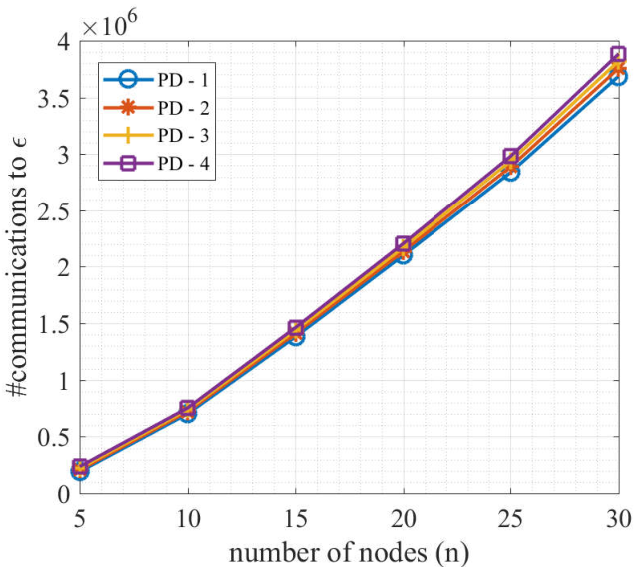
In order to study the performance of our proposed framework on different networks, we consider agents which are connected with random regular graphs (agents first form a ring and then each agent gets connected to two other random agents). The objective function at each agent is of the form with and being integers that are randomly chosen from and . We run the simulation for random seeds and we plot the average number of steps and communications until the relative error is less than , i.e., in Figure 2. The method of multipliers (centralized implementation) is also included as a benchmark. The primal stepsize parameter at each seed is chosen based on the theoretical bound given in Eq. (14) and the dual stepsize is . We observe that regardless the size of network, increasing the number of primal updates per iteration improves the performance of the algorithm. We also observe that as the network size grows, the number of steps to optimality of our proposed method grows sublinearly and the communication needed increases almost linearly. In our simulations, we use the mushrooms dataset [6], with data points, distributed uniformly over agents. Each data point has a feature vector of size and a label which is either or . In Figure 1 we compare the performance of our primal-dual algorithms [c.f. Algorithm 1] with (represented by PD - 1 to PD - 4), with EXTRA [31], DIGing [23], and NEAR-DGD+ [1], in terms of relative error, , with respect to number of iterations and number of communications. The benchmark is computed using minFunc software [30] and the stepsize parameters are manually tuned for each algorithm. We can clearly see that increasing the number of primal updates improves the performance of the algorithm, while incurring a higher communication cost. In our experiments, we observed that by increasing to larger numbers, the performance of the algorithms does not improve much, which can be explained through Remark 3 and also the effect of the outdated gradients. EXTRA and DIGing algorithms are special cases of our algorithm for specific choices of matrices and and one primal update per iteration, and thus have close performance to PD - 1. In the NEAR-DGD+ the number of communications increases linearly with the iteration number, which results in slow convergence with respect to the number of communications. We obtained similar results for other standard machine learning datasets, including diabetes-scale, heart-scale, a1a, australian-scale, and german [6].

V Final Remarks
In this paper we propose a general framework of first order decentralized primal-dual optimization algorithms. Our general class of algorithms allows for multiple primal updates per iteration, which results in design flexibility to control the trade off between execution complexity and performance of the algorithm. We show that the proposed class of algorithms converges to the exact solution with a global linear rate. The numerical experiments show the convergence speed improvement of primal-dual algorithms with multiple primal updates per iteration compared to other known first order methods like EXTRA, DIGing, and NEAR-DGD+. Possible future work includes analysis of the convergence properties for non-convex objective functions and extending the framework to second order primal-dual algorithms.
References
- [1] Albert Berahas, Raghu Bollapragada, Nitish Shirish Keskar, and Ermin Wei. Balancing communication and computation in distributed optimization. IEEE Transactions on Automatic Control, 2018.
- [2] Dimitri P Bertsekas. Incremental gradient, subgradient, and proximal methods for convex optimization: A survey. Optimization for Machine Learning, 2010(1-38):3, 2011.
- [3] Dimitri P Bertsekas. Constrained optimization and Lagrange multiplier methods. Academic press, 2014.
- [4] Dimitris Bertsimas and John N Tsitsiklis. Introduction to linear optimization, volume 6. Athena Scientific Belmont, MA, 1997.
- [5] Stephen Boyd, Neal Parikh, Eric Chu, Borja Peleato, Jonathan Eckstein, et al. Distributed optimization and statistical learning via the alternating direction method of multipliers. Foundations and Trends® in Machine learning, 3(1):1–122, 2011.
- [6] Chih-Chung Chang and Chih-Jen Lin. LIBSVM: a library for support vector machines. ACM transactions on intelligent systems and technology (TIST), 2(3):27, 2011.
- [7] Annie I Chen and Asuman Ozdaglar. A fast distributed proximal-gradient method. In Communication, Control, and Computing (Allerton), 2012 50th Annual Allerton Conference on, pages 601–608. IEEE, 2012.
- [8] Mark Eisen, Aryan Mokhtari, and Alejandro Ribeiro. Decentralized quasi-Newton methods. IEEE Transactions on Signal Processing, 65(10):2613–2628, 2017.
- [9] Magnus R Hestenes. Multiplier and gradient methods. Journal of optimization theory and applications, 4(5):303–320, 1969.
- [10] Franck Iutzeler, Pascal Bianchi, Philippe Ciblat, and Walid Hachem. Explicit convergence rate of a distributed alternating direction method of multipliers. IEEE Transactions on Automatic Control, 61(4):892–904, 2016.
- [11] Dušan Jakovetić, José MF Moura, and Joao Xavier. Linear convergence rate of a class of distributed augmented lagrangian algorithms. IEEE Transactions on Automatic Control, 60(4):922–936, 2015.
- [12] Dušan Jakovetić, Joao Xavier, and José MF Moura. Fast distributed gradient methods. IEEE Transactions on Automatic Control, 59(5):1131–1146, 2014.
- [13] Vassilis Kekatos and Georgios B Giannakis. Distributed robust power system state estimation. IEEE Transactions on Power Systems, 28(2):1617–1626, 2013.
- [14] Qing Ling, Wei Shi, Gang Wu, and Alejandro Ribeiro. DLM: Decentralized linearized alternating direction method of multipliers. IEEE Trans. Signal Processing, 63(15):4051–4064, 2015.
- [15] Fatemeh Mansoori and Ermin Wei. Superlinearly convergent asynchronous distributed network Newton method. In Decision and Control (CDC), 2017 IEEE 56th Annual Conference on, pages 2874–2879. IEEE, 2017.
- [16] Aryan Mokhtari, Qing Ling, and Alejandro Ribeiro. Network Newton-part i: Algorithm and convergence. arXiv preprint arXiv:1504.06017, 2015.
- [17] Aryan Mokhtari and Alejandro Ribeiro. DSA: Decentralized double stochastic averaging gradient algorithm. The Journal of Machine Learning Research, 17(1):2165–2199, 2016.
- [18] Aryan Mokhtari, Wei Shi, Qing Ling, and Alejandro Ribeiro. Decentralized quadratically approximated alternating direction method of multipliers. In Signal and Information Processing (GlobalSIP), 2015 IEEE Global Conference on, pages 795–799. IEEE, 2015.
- [19] Aryan Mokhtari, Wei Shi, Qing Ling, and Alejandro Ribeiro. A decentralized second-order method with exact linear convergence rate for consensus optimization. IEEE Transactions on Signal and Information Processing over Networks, 2(4):507–522, 2016.
- [20] Joao FC Mota, Joao MF Xavier, Pedro MQ Aguiar, and Markus Puschel. D-ADMM: A communication-efficient distributed algorithm for separable optimization. IEEE Transactions on Signal Processing, 61(10):2718–2723, 2013.
- [21] Angelia Nedić. Asynchronous broadcast-based convex optimization over a network. IEEE Transactions on Automatic Control, 56(6):1337–1351, 2011.
- [22] Angelia Nedić and Dimitri Bertsekas. Convergence rate of incremental subgradient algorithms. In Stochastic optimization: algorithms and applications, pages 223–264. Springer, 2001.
- [23] Angelia Nedić, Alex Olshevsky, and Wei Shi. Achieving geometric convergence for distributed optimization over time-varying graphs. SIAM Journal on Optimization, 27(4):2597–2633, 2017.
- [24] Angelia Nedić, Alex Olshevsky, and Wei Shi. Improved convergence rates for distributed resource allocation. In 2018 IEEE Conference on Decision and Control (CDC), pages 172–177. IEEE, 2018.
- [25] Angelia Nedić and Asuman Ozdaglar. Distributed subgradient methods for multi-agent optimization. IEEE Transactions on Automatic Control, 54(1):48–61, 2009.
- [26] Joel B Predd, Sanjeev R Kulkarni, and H Vincent Poor. Distributed learning in wireless sensor networks. John Wiley & Sons: Chichester, UK, 2007.
- [27] S Sundhar Ram, A Nedić, and Venugopal V Veeravalli. Incremental stochastic subgradient algorithms for convex optimization. SIAM Journal on Optimization, 20(2):691–717, 2009.
- [28] S Sundhar Ram, Angelia Nedić, and Venugopal V Veeravalli. Distributed stochastic subgradient projection algorithms for convex optimization. Journal of optimization theory and applications, 147(3):516–545, 2010.
- [29] Wei Ren, Randal W Beard, and Ella M Atkins. Information consensus in multivehicle cooperative control. IEEE Control systems magazine, 27(2):71–82, 2007.
- [30] Mark Schmidt. minfunc: unconstrained differentiable multivariate optimization in matlab. Software available at http://www. cs. ubc. ca/˜ schmidtm/Software/minFunc. htm, 2005.
- [31] Wei Shi, Qing Ling, Gang Wu, and Wotao Yin. EXTRA: An exact first-order algorithm for decentralized consensus optimization. SIAM Journal on Optimization, 25(2):944–966, 2015.
- [32] Wei Shi, Qing Ling, Kun Yuan, Gang Wu, and Wotao Yin. On the linear convergence of the ADMM in decentralized consensus optimization. IEEE Trans. Signal Processing, 62(7):1750–1761.
- [33] Konstantinos I Tsianos, Sean Lawlor, and Michael G Rabbat. Consensus-based distributed optimization: Practical issues and applications in large-scale machine learning. In 2012 50th Annual Allerton Conference on Communication, Control, and Computing (Allerton), pages 1543–1550. IEEE, 2012.
- [34] Rasul Tutunov, Haitham Bou Ammar, and Ali Jadbabaie. A distributed Newton method for large scale consensus optimization. arXiv preprint arXiv:1606.06593, 2016.
- [35] Ermin Wei and Asuman Ozdaglar. Distributed alternating direction method of multipliers. 2012.
- [36] Ermin Wei and Asuman Ozdaglar. On the O(1/k) convergence of asynchronous distributed alternating direction method of multipliers. In Global conference on signal and information processing (GlobalSIP), 2013 IEEE, pages 551–554. IEEE, 2013.
- [37] Tianyu Wu, Kun Yuan, Qing Ling, Wotao Yin, and Ali H Sayed. Decentralized consensus optimization with asynchrony and delays. IEEE Transactions on Signal and Information Processing over Networks, 4(2):293–307, 2018.
- [38] Lin Xiao and Tong Zhang. A proximal stochastic gradient method with progressive variance reduction. SIAM Journal on Optimization, 24(4):2057–2075, 2014.