Maxwell electrodynamics modified by a CPT-odd
dimension-five higher-derivative term
Abstract
In this paper, we consider an electrodynamics of higher derivatives coupled to a Lorentz-violating background tensor. Specifically, we are interested in a dimension-five term of the CPT-odd sector of the nonminimal Standard-Model Extension. By a particular choice of the operator , we obtain a higher-derivative version of the Carroll-Field-Jackiw (CFJ) term, , with a Lorentz-violating background vector . This modification is subject to being investigated. We calculate the propagator of the theory and from its poles, we analyze the dispersion relations of the isotropic and anisotropic sectors. We verify that classical causality is valid for all parameter choices, but that unitarity of the theory is generally not assured. The latter is found to break down for certain configurations of the background field and momentum. In an analog way, we also study a dimension-five anisotropic higher-derivative CFJ term, which is written as and is directly linked to the photon sector of Myers-Pospelov theory. Within the second model, purely timelike and spacelike are considered. For the timelike choice, one mode is causal, whereas the other is noncausal. Unitarity is conserved, in general, as long as the energy stays real — even for the noncausal mode. For the spacelike scenario, causality is violated when the propagation direction lies within certain regimes. However, there are particular configurations preserving unitarity and strong numerical indications exist that unitarity is guaranteed for all purely spacelike configurations. The results improve our understanding of nonminimal CPT-odd extensions of the electromagnetic sector.
pacs
11.30.Cp, 12.60.-i, 03.70.+k, 11.55.FvI Introduction
The minimal Standard-Model Extension (SME), which was proposed by V.A. Kostelecký and S. Samuel in 1998 Colladay; Samuel, shares various established properties with the Standard Model (SM) such as power-counting renormalizability, energy-momentum conservation, and gauge invariance. However, it does not preserve Lorentz symmetry and, beyond that, it can violate CPT symmetry Greenberg:2002uu. The SME is an effective field-theory framework obtained from the SM including additional terms composed of observer Lorentz-invariant contractions of the physical SM fields and fixed background tensors. Studies based on the SME have been carried out to look for Lorentz-violating (LV) effects and to develop a precision program that may allow us to examine the limitation of Lorentz symmetry in various physical interactions. In this sense, a large number of investigations has been realized in the context of the fermion sector Fermion1; Fermion2; Fermion3, CPT symmetry violation CPT, the electromagnetic CPT-odd sector Adam1; Adam2; Cherenkov1, the electromagnetic CPT-even sector Cherenkov2; KM, photon-fermion interactions KFint; Interac; Schreck1, and radiative corrections Radio1; Radio2; Radio3. Phenomenological and theoretical developments focusing on LV contributions of mass dimensions 3 and 4 have been continuously undertaken in the latest years. As a result, there is now a large number of tight constraints on Lorentz violation, mainly in the photon and lepton sector KostRussell.
To enable theoretical predictions of quantum-gravity effects at energies much smaller than the Planck scale, we must assume that such a fundamental theory has a perturbative expansion in terms of the dimensionless ratio . Here, is the energy of some experiment of interest and is the mass scale where the full theory of quantum gravity must be considered to describe the physics as a whole. The latter is expected to be related to the Planck mass; at least it is supposed to lie in its vicinity: . In configuration space, a single power of energy corresponds to a spacetime derivative that occurs in an appropriate field operator. Based on the existence of such an asymptotic expansion, the SM described by the Lagrange density can be interpreted as a zeroth-order contribution of this series. The SM depends on a range of different mass scales such as the electron mass , the proton mass or the electroweak mass scale . In what follows, we will choose as its characteristic mass scale.
The difference between the minimal SME and the SM is that the former involves Lorentz-violating controlling coefficients that are either of mass dimension 1 or dimensionless. They are contracted with field operators of mass dimension 3 and 4, respectively (incorporated in ).11 1 The standard notation employed is to indicate the mass dimensions of the corresponding field operators as indices in parentheses. For dimensional reasons and to take into account a suppression of Lorentz violation by the scale , the dimension-four coefficients could be formed via appropriate constant ratios such as . These contributions do not rise with energy, which is why formally they also must be considered as of zeroth order. The properties of the dimension-three coefficients are peculiar in this sense. Following the previous arguments, they should be of order , i.e., they ought to have a dependence of the form . Hence, they are expected to be suppressed for increasing energies, but for energies small enough, they would be large due to the occurrence of the quantum-gravity mass scale in the numerator. Obviously, there is no experimental evidence for Lorentz violation that big, whereupon these terms must be suppressed in a different manner.
Taking into account contributions that grow with energy, naturally leads us to power-counting nonrenormalizable theories. There may be Lorentz-invariant terms (contained in ) that are suppressed by a mass scale not necessarily related to the Planck mass. As these terms are Lorentz-invariant, their origin might lie in a regime different from that of Planck-scale physics. They are also known to improve the ultraviolet behavior of theories, which was certainly one of the main motivations for exploring such terms (see below).
In the latest years, an interplay between Lorentz violation and theories endowed with higher derivatives has taken place. Indeed, Lorentz violation can incorporate operators of higher mass dimensions, which may include higher-derivative terms. The number of such contributions is infinite in contrast to the minimal LV extensions. Nonminimal versions of the SME were developed for both the photon Kostelec1 and the fermion sector Kostelec2; Joao. The Lorentz-violating contributions are supposedly suppressed by powers of the Planck scale and are comprised by the Lagrange density of the nonminimal SME. So we can write the asymptotic series in the form
| (1a) | ||||
| (1b) | ||||
| (1c) | ||||
| (1d) | ||||
Here, we also stated the general structure of individual terms. A generic dimensionless background tensor with a set of Lorentz indices is indicated by where is a field operator with the same set of Lorentz indices. The mass dimension of the background has been extracted explicitly to show the dependence on the scales and . The remaining Lagrange density contains all additional contributions that have not been taken into account previously. These could be nonperturbative in nature.
According to the perturbative series of Eq. (1), the nonminimal SME is a natural extension of the higher-derivative Lorentz-invariant contributions in the same sense as the minimal SME is an extension of the SM. Searching for physics beyond the SM via an effective theory, there is a priori no reason why such nonminimal terms should be discarded. Interpreting these terms as theories that are valid within a certain energy range only, power-counting nonrenormalizability is not considered to be a problem.
Due to the arguments explained above, individual terms have an energy dependence of the form and , respectively. Nonminimal contributions grow with energy, i.e., after a certain point they dominate the minimal ones. Therefore, they might be essential in experiments involving particles of high energies, e.g., cosmic rays. From the theoretical perspective, fundamental properties such as causality, stability, and unitarity could be investigated in the high-energy regime where the higher-derivative field operators become dominant. In what follows, we will state several examples for nonrenormalizable extensions of electrodynamics that are Lorentz-invariant.
The first example of an extended electrodynamics including higher derivatives was proposed in 1942 by Podolsky Podolsky1. He initially studied the Lorentz- and gauge-invariant dimension-6 term, , with the Podolsky parameter of mass dimension . This theory exhibits two dispersion relations, the usual one of Maxwell theory and a massive mode that renders the self-energy of a pointlike charge finite. However, at the quantum level, the massive mode produces ghosts Accioly1. The gauge-fixing condition for this extension can be adapted to be compatible with the 2 degrees of freedom of the photon and the 3 additional ones connected to the massive mode GalvaoP. Further developments Podolsky3; Podolsky5 in Podolsky’s theory deserve to be mentioned including investigations of a dimension-six quantum electrodynamics in (1+1) spacetime dimensions Manavella.
Another relevant extension of Maxwell theory with higher derivatives is Lee-Wick electrodynamics, described by the dimension-6 term LeeWick. This theory also implies a finite self-energy for a pointlike charge in spacetime dimensions. It provides a bilinear contribution to the Maxwell Lagrangian that is similar to the Podolsky term but with opposite sign. This term causes energy instabilities at the classical level and negative-norm states in the Hilbert space at the quantum level. Lee and Wick introduced a mechanism to preserve unitarity by removing all states with negative norm from the Hilbert space. Ten years ago, this theory received attention again with the proposal of the Lee-Wick Standard Model LW, which is based on a non-Abelian gauge structure free of quadratic divergences. The Lee-Wick Standard Model has had a big impact and is applied in both theory and phenomenology LW2. In this context, general investigations of LV extensions are found in Turcati as well as applications to the self-energy and interaction of pointlike and spatially extended sources Barone2; Accioly2; Barone1; Barone3. General considerations of the pole structure and perturbative unitarity of these classes of theories can be found in Anselmi.
As we explained above, theories of higher derivatives and higher-derivative electrodynamics, in particular, can be endowed with Lorentz-violating contributions. It is important to mention that special choices of nonminimal operators were proposed and investigated Myers1; Marat; Reyes:2010pv; Reyes:2013nca where some works such as Passos even involve Hořava-Lifshitz gravity. Nonminimal theories containing higher-dimensional couplings can also be constructed without introducing higher derivatives (beyond those contained inside the field strength tensor). Such couplings were considered and constrained initially in NModd1; NM3 and have been proposed recently in broader scenarios NMkost; NMkost2, also including photon-photon scattering Gomes, electroweak interactions VictorEW, nuclear chiral interactions VictorCar, scalar electrodynamics Josberg, and scattering processes of electrons and positrons Khanna.
Another motivation to studying higher-derivative Lorentz-violating terms are noncommutative spacetime theories. These are based on commutation relations for spacetime coordinates of the form . The object is fixed with respect to particle Lorentz transformations and is interpreted as an observer tensor giving rise to preferred spacetime directions. Due to dimensional reasons, , whereupon it is inevitable that this object must be linked to terms of the nonminimal SME. This property was shown explicitly in Carroll:2001ws by applying the Seiberg-Witten map to translate a noncommutative field theory into a commutative field theory of modified photons.
Lately, modified higher-derivative LV terms have been generated in other ways via quantum corrections to the photon effective action in a scenario with a nonminimal coupling between fermions and photons PetrovPLB2016; Barone4 as well as in supersymmetric theories Bonetti1; Bonetti2. Recently, dimension-five terms of Myers-Pospelov type have been investigated in the context of black-body radiation Anacleto and emission of electromagnetic and gravitational waves Anacleto2. Higher-derivative applications to gamma rays have also been taken into consideration Gamma. Not so long ago, we addressed a CPT-even, dimension-6, higher-derivative electrodynamics, composed of an anisotropic Podolsky term, , and an anisotropic Lee-Wick term, , respectively, with representing a LV rank-2 background field. Both models can be mapped onto dimension-6 terms of the electromagnetic sector within the SME. We obtained the associated gauge propagators and examined the dispersion relations for several background tensor configurations. We found that both models exhibit both causal and noncausal as well as both unitary and nonunitary modes Leticia1.
To improve our understanding of higher-derivative Lorentz-violating extensions of the photon sector, it is now reasonable to pursue similar investigations of a CPT-odd theory. Therefore, in the present work, we study Maxwell electrodynamics modified by a CPT-odd, dimension-five nonminimal SME term. In Sec. II, we consider a configuration composed of a fixed background field where the additional four-derivatives are contracted with the metric tensor, i.e., . The gauge propagator is derived and the dispersion relations are obtained from its pole structure. Causality and unitarity of the modes is analyzed subsequently. In Sec. III, we analyze an alternative configuration composed of a fixed background field partially contracted with additional four-derivatives, that is, . Similar investigations are performed for this more sophisticated modification that is linked to the photon sector of Myers-Pospelov theory. Finally, we conclude on our findings in Sec. IV. Studies that are not directly connected to the modifications proposed are relegated to Appx. A, B. Natural units will be used with , unless otherwise stated.
II Maxwell electrodynamics modified by a CPT-odd dimension-five higher-derivative term: a simple model
The Lagrange density for the nonminimal SME photon sector Kostelec1 is written in a way similar to that of the minimal sector:
| (2) |
with the U(1) gauge field and the associated field strength tensor . The four-dimensional Levi-Civita symbol is denoted by where we use the convention . All fields are defined in Minkowski spacetime with metric tensor . The operators and now represent the nonminimal versions of the corresponding minimal coefficients and . They involve terms of higher derivatives and are given by the following infinite CPT-odd and CPT-even operator series:
| (3a) | ||||
| (3b) | ||||
Each controlling coefficient is labeled by the mass dimension of the associated field operator and the Lorentz indices are associated with the spacetime derivatives. In this work, we are interested in investigating the CPT-odd, dimension-five extension of the electromagnetic sector that is specifically represented by the Carroll-Field-Jackiw-like (CFJ-like) term of the Lagrange density:
| (4) |
The background field is a third-rank observer Lorentz tensor whose general structure is
| (5) |
As a first investigation, we consider the special case
| (6) |
with a Lorentz-violating four-vector . The tensor structure is chosen such that the vector properties of are described by the preferred spacetime direction , whereas the nonminimal sector is separately parameterized by the symmetric tensor . Thus, the Maxwell-Carroll-Field-Jackiw-like (MCFJ-like) Lagrange density to be studied is
| (7) |
with gauge fixing parameter , i.e., the final term is included to fix the gauge. We can consider an observer frame where is diagonal. In this context, the simplest case is that of a tensor with equal spacelike coefficients. Then is composed of a traceless part and a part with nonvanishing trace that must be proportional to the Minkowski metric tensor:
| (8a) | ||||
| (8b) | ||||
| with the preferred purely timelike direction and parameters , suitably chosen.22 2 Here we simply adopt the notation used in the CPT-even photon sector where the single coefficient is linked to a symmetric, traceless matrix, as well. As the traceless part involves two preferred directions and , its investigation is probably more complicated than that of the contribution proportional to the trace. Therefore, we leave the analysis of the traceless part for the future and choose so that , with the d’Alembertian and the redefined background vector . Thus, the LV background is | ||||
| (8c) | ||||
| and the new Lagrange density has the form | ||||
| (9) |
By performing suitable partial integrations and neglecting boundary terms, the latter can be written as
| (10a) | |||
| with the differential operator | |||
| (10b) | |||
sandwiched in between two vector fields. Here we introduced the symmetric transversal and longitudinal projectors, and , respectively:
| (11) |
while the Lorentz-violating part is described by the antisymmetric and dimensionless operator,
| (12) |
Now we intend to evaluate the propagator of the theory, i.e., we should find the Green’s function , which is the inverse of the differential operator , from the condition
| (13) |
For the inverse to be found, we use a suitable basis of tensor operators, a procedure that turned out to be successful in several theoretical scenarios Propagator; Propagator2. Thus, we propose the following Ansatz:
| (14) |
where the parameters are expected to be scalar operators. The algebra of the individual tensor operators is displayed in Table 1. We also use the definition
| (15) |
and, for brevity, define the tensor
| (16) |
which originates from the contraction of two Levi-Civita symbols.
| 0 | 0 | ||||||
| 0 | 0 | 0 | 0 | ||||
| 0 | 0 | 0 | 0 | ||||
| 0 | 0 | 0 | |||||
| 0 | 0 | ||||||
| 0 | 0 | 0 | |||||
| 0 | 0 |
Starting from the tensor equation (13), after performing some simplifications, we have
| (17) |
By comparing both sides of Eq. (17) to each other, the following differential operators are obtained:
| (18a) | ||||
| (18b) | ||||
| (18c) | ||||
| (18d) | ||||
Thus, the inverse of is
| (19) |
The form of the propagator in momentum space follows from the latter result by carrying out the substitution with the four-momentum , so that:
| (20a) | ||||
| with | ||||
| (20b) | ||||
A prefactor of has been added to match the conventions for the photon propagator for zero Lorentz violation in Peskin:1995. Several remarks are in order. First, in App. A we present the propagator of MCFJ theory in Lorenz gauge, showing that the latter and Eq. (20) are linked to each other by a simple replacement. Second, the propagator (20) is transverse, except for a piece that depends on the gauge-fixing parameter:
| (21) |
Third, note that contributions of the form (with the four-momentum replaced by the four-velocity ) appear in the context of certain classical Lagrangians associated with the SME, especially in those that arise for the coefficients (connected to Finsler space) Finsler. In Euclidean space, this quantity corresponds to the Gramian of the two vectors that appear in the expression. As there is a connection between the CPT-odd electromagnetic sector and the coefficients of the fermionic sector, such quantities are expected to appear. The structure of was also observed in the graviton propagator evaluated in the context of the linearized Einstein-Hilbert gravity (without torsion) modified by a spontaneous violation of Lorentz symmetry. The latter is induced by the bumblebee field MalufGravity; MalufGravity2 using generalized versions of the Barnes-Rivers spin operator basis Barnes; Rivers; Sezgin. Finally, note that is a dimensionless function, as the mass dimension of cancels the inverse mass dimension of .
Fourth, it is interesting to recall that the propagator (20a) has an antisymmetric term, proportional to the projector while the other pieces are symmetric with respect to the interchanges , . The Feynman propagator33 3 Note that we did not determine the Feynman propagator here, as the latter requires the definition of a suitable pole structure. The Feynman propagator is mentioned to emphasize the symmetries that must be the same as those of the Green’s function. is defined by the vacuum expectation value of the time-ordered product of field operators evaluated at distinct spacetime points,
| (22) |
The Fourier transform of the latter is symmetric with respect to the combination of interchanging its indices and . The antisymmetric piece of the propagator (20a) appears in CPT-odd electrodynamics, e.g., in the MCFJ model or Chern-Simons theory in (1+2) dimensions. But this piece does not mean that the propagator loses its symmetry. Indeed, the propagator continues being symmetric with regards to the two simultaneous operations mentioned before.
II.1 Dispersion relations
The poles of the propagator provide two dispersion equations for this model,
| (23a) | ||||
| (23b) | ||||
| as usual in theories with higher-dimensional operators. The first one corresponds to the typical Maxwell pole, which also appears in the Podolsky and Lee-Wick models as well as in the corresponding anisotropic LV versions Leticia1. The second equation contains information on the higher-derivative dimension-five term. It is reasonable to compare it to the dispersion equation obtained for the dimension-three MCFJ theory (see Eq. (25) in the first paper of Adam1), given in terms of the CFJ background vector : | ||||
| (24) |
The latter is a quartic-order dispersion equation, whereas Eq. (23b) is simpler (only of second order). Such a comparison reveals that the present dimension-five MCFJ-like theory is totally distinct from the dimension-three MCFJ model. The less involved dispersion equation can be ascribed to the simple structure of the background tensor that we have chosen in Eq. (6).
We will analyze the dispersion relations (DRs) for several configurations of the LV background where it makes sense to distinguish between purely timelike and spacelike preferred directions. If a DR does not approach the limit of standard electromagnetic waves for zero Lorentz violation, it will be called “exotic.” The latter are not necessarily unphysical, but they decouple in the low-energy regime. Dispersion laws whose group/front velocities are singular or exceed the value 1 will be referred to as “spurious.” For a purely timelike background, , we have
| (25) |
which does not correspond to a propagating mode. It is a nonphysical DR, as it does not represent a relation between energy and momentum. Thus, there is no propagating mode associated with a timelike background vector. This property is an important difference between the dimension-five model under consideration and MCFJ theory. The latter exhibits a DR associated with a timelike background vector. However, this timelike sector is plagued by consistency problems Adam1.
Now, for a purely spacelike background, , the corresponding DR is
| (26) |
which can also be written as
| (27a) | |||
| with the angle enclosed by and : | |||
| (27b) | |||
| This is a DR that is compatible with the propagation of signals, whose properties need to be examined. In the current section, we are especially interested in classical causality that is characterized by the behavior of the group and front velocity and , respectively, where Brillouin:1960 | |||
| (28) |
Classical causality is established as long as both and . We now evaluate these characteristic velocities for DR (26). The front velocity is
| (29) |
as . Furthermore, we investigate the behavior of the group velocity:
| (30) |
whose magnitude is
| (31) |
where is a dimensionless parameter. Large momenta correspond to large . Hence,
| (32) |
independently of the angle . As and , classical causality is established for the whole range of LV coefficients and momenta. Figure 1 presents the behavior of the magnitude of the group velocity. The graph shows a monotonically increasing group velocity that reaches the asymptotic value 1, which is a behavior in accordance with causality. It shares this property with the spacelike sector of MCFJ theory where classical causality is guaranteed, as well (see first paper of Adam2). The mode obtained here is exotic in the sense that it does not propagate when Lorentz violation goes to zero. Hence, it does not approach the standard DR in this limit. The mode must be understood as a high-energy effect that propagates in a well-behaved manner for large momenta.
II.2 Unitarity
The next step is to study unitarity at tree-level, which is performed by means of the saturated propagator SP Veltman. The latter is a scalar quantity that is implemented by contracting the propagator with external physical currents as follows:
| (33) |
The current is assumed to be real and satisfies the conservation law , which in momentum space reads . In accordance with this method, unitarity is assured whenever the imaginary part of the residue of the saturation SP (evaluated at the poles of the propagator) is nonnegative. A way of carrying out the calculation is to determine the eigenvalues of the propagator matrix, evaluated at their own poles with current conservation taken into account. For the propagator found in Eq. (20), the saturation is
| (34) |
where . Contracting the propagator with two equal conserved currents corresponds to getting rid of all gauge-dependent (and therefore, unhysical) contributions. These usually are terms that involve four-momenta with free indices corresponding to the indices of the Green’s function. Although the term does not have this structure, it vanishes when coupled to two external conserved currents due to its antisymmetry. Hence, the only Lorentz-violating contributions of the propagator that have an impact on unitarity (based on our criterion) are the denominators and the symmetric term, , formed from a combination of two preferred spacetime directions.
Now, for the Maxwell pole, , the residue of the saturation is
| (35) |
At the pole it holds that . From the law of current conservation we obtain . Therefore, we can cast the corresponding imaginary part into the form
| (36) |
For any background, , the imaginary part of the saturation (36) is nonnegative for small momenta, but becomes negative as the momentum increases. For a timelike configuration, , and for a spacelike configuration, , the quantity (36) becomes negative for and , respectively. So, unitarity is not assured at the pole for all configurations possible.
For the second DR, Eq. (23b), it only makes sense to examine the spacelike configuration, , where
| (37) |
It is reasonable to write the saturation as
| (38) |
Its residue at this pole is
| (39) |
Due to current conservation, , the four-current squared can be cast into
| (40) |
In the standard case, current conservation implies that , i.e., any physical four-current is spacelike. However, this property does not necessarily hold in Lorentz-violating theories, anymore — as shown by Eq. (40). Inserting this result into Eq. (39), leads to the residue
| (41) |
There are configurations for which the imaginary part of the latter is positive. For example, we can choose parallel to , whereby Eq. (41) reduces to
| (42) |
The first (negative) term can be suppressed for large momenta as long as . As the second (positive) contribution does not depend on the momentum, the imaginary part of the residue can be positive for large enough momenta. Hence, there are configurations of background field, large momenta, and external current for which unitarity is valid. This behavior is in accordance with the previous interpretation that the mode is exotic and must be interpreted as a high-energy effect. In a more specific way, if is the angle between and , we have and . Thus, the residue (42) reads
| (43) |
whose imaginary part is positive for
| (44) |
The latter condition assures unitarity. A more general case to be investigated is with , for which and . To examine it, we exploit observer rotation invariance and employ the following coordinate system:
| (45) |
in which
| (46a) | ||||
| (46b) | ||||
where is the angle between the axis and the projection of the vector in the - plane.44 4 Note that there is no connection between the axis used here and the variable employed previously, e.g., in Eq. (31). For this configuration, the residue (41) can be expressed as
| (47) |
The imaginary part of the latter is always negative, which demonstrates unitarity violation for any choice of the momentum and the angles. A similar investigation for yields a residue whose imaginary part can be either positive or negative, also providing unitarity violation in some situations.
To summarize, while causality is assured for any configuration of the purely spacelike background, unitarity can hold, but does not do so necessarily. In the next section we will examine a more involved version of this first higher-derivative model.
III Maxwell electrodynamics modified by a CPT-odd dimension-five higher-derivative term: a second model
In the last section, we have examined a CPT-odd, dimension-five, nonminimal extension of the electromagnetic sector, specifically represented by the CFJ-like Lagrange density
| (48) |
where the background vector field was written according to Eq. (8c). As a second possibility, we propose the more sophisticated choice
| (49) |
where is a Lorentz-violating four-vector whose mass dimension is
| (50) |
or equivalently . In contrast to the theory studied before, the vectorlike background field is now also contracted with the additional derivatives. This structure is supposed to render the properties of the current theory more involved than those of the previously studied one. Modifying Maxwell’s theory by including this term into its Lagrange density, leads to a higher-derivative (dimension-five) anisotropic MCFJ-like theory described by
| (51) |
In App. B we establish the connection between the modifications given by Eqs. (9), (51) and the very general compilation of Lorentz-violating contributions listed in NMkost2. Now, the latter Lagrangian can also be written as
| (52a) | |||
| with the operator | |||
| (52b) | |||
sandwiched between two gauge fields. Note that Eq. (51) is directly linked to the photon sector of Myers-Pospelov theory (cf. the first paper of Myers1). The latter was initially constructed as a prototype of higher-derivative Lorentz-violating theories and includes dimension-five modifications of scalars, Dirac fermions, and photons. In Reyes:2010pv; Reyes:2013nca, certain properties of its photon sector are on the focus. Our Eq. (51) corresponds to the theory studied in the latter references for the correspondence (with their coupling constant and preferred direction ) and the choice of the gauge fixing parameter. The article Reyes:2010pv is primarily dedicated to studying classical causality. Unitarity is analyzed in Reyes:2013nca for a lightlike background vector based on the validity of the optical theorem at tree-level. In what follows, we intend to discuss additional aspects of classical causality of this particular theory. Furthermore, the forthcoming investigation of unitarity is new in the sense that it relies on a different technique (investigation of the residues of the saturated propagator) and it is carried out for different sectors of the theory (timelike and spacelike preferred directions ).
Now, comparing the operator of (52b) to that of Eq. (10b), it is no longer possible to extract a d’Alembertian from it. The projectors , are given as before by Eq. (11) and the Lorentz-violating antisymmetric operator now reads
| (53) |
To determine the propagator of the theory given by Eq. (51), we propose the following Ansatz:
| (54) |
that must satisfy the identity
| (55) |
The algebra of the tensor operators , , , , , and is the same as that presented in Tab. 1 with the replacement to be performed. For brevity, we introduce
| (56a) | ||||
| (56b) | ||||
To find the scalar operators , we start from the tensor equation (55) and employ the algebra of the tensor operators as before. The calculation is completely analogous. After performing some algebraic simplifications, we obtain
| (57a) | |||
| where | |||
| (57b) | |||
The form of the propagator in momentum space is:
| (58) |
As before, the parts of the propagator independent of the gauge-fixing parameter are transversal, i.e., the result of Eq. (21) can be carried over. Taking into account the correspondence and the choice , we found that our of Eq. (58) corresponds to Eq. (72) of Reyes:2010pv.
III.1 Dispersion relations
As observed in the first model, the propagator poles provide two dispersion equations, namely
| (59a) | ||||
| (59b) | ||||
The first again corresponds to the usual Maxwell pole, while the second involves LV modifications caused by the higher-derivative term. We will analyze the second dispersion equation for two configurations of the LV background, which exhibit preferred directions in a spacetime modified by Lorentz violation. We need to notice that the dispersion equation (59b) is different from Eq. (23b), as it still makes sense when the LV coefficient vanishes, whereas expression (23b) does not. Hence, the classification “exotic” will be not used here. A DR originating from Eq. (59b) can be named spurious, when it exhibits unphysical behavior, or unconventional, when it is well-behaved. For a purely timelike background, , we have
| (60) |
which is equal to Eq. (19) in Reyes:2010pv. In contrast to the first model, there are now two distinct modified modes. The notation refers to the mode with the plus and minus sign label, respectively. The energy is well-defined for the mode , but not for the mode , for which it is only meaningful as long as . Furthermore, a sign change of the controlling coefficient simply interchanges the two DRs. Hence, without restriction of generality, we assume a nonnegative coefficient: .
On the other hand, for a purely spacelike background, , the corresponding DR is
| (61a) | |||
| with the angle enclosed by and : | |||
| (61b) | |||
The latter is confirmed by Eq. (29) in Reyes:2010pv when the appropriate replacements are carried out. Recall that , , have mass dimension equal to 2, while is dimensionless. It is possible to show that the energy (61a) is real for any absolute value of the background vector and direction relative to , that is, . Besides, the DR of the mode is mapped to that of the mode and vice versa when the direction of is reversed, i.e., when or . When electromagnetic waves propagate along a direction perpendicular to , Lorentz violation does not have any effect and the DR is standard. In the suitable momentum range, Eqs. (60) and (61a) represent DRs compatible with a propagation of signals.
As before, we investigate classical causality via the group and front velocity and , respectively, defined in Eq. (28). We now evaluate these characteristic velocities for DRs originating from the dispersion equation (59b). On the one hand, we compute the front velocity for DR (60). For the mode , the latter is not defined, as the energy becomes complex for momenta beyond . For the mode , we obtain
| (62) |
On the other hand, we evaluate the group velocity:
| (63) |
whose absolute values read (cf. also Eq. (21) in Reyes:2010pv)
| (64) |
where only makes sense for the range of momenta , which is the same range that assures real energies for this mode. The behavior of is depicted in Fig. 2. The large-momentum limit of the group velocity for the mode is simply given by
| (65) |
The results for the front and group velocity indicate that signals do not propagate for large momenta. Furthermore, is well-behaved for all momenta, whereas exhibits a singularity at . For , classical causality breaks down for this mode. Thus, the mode must be considered as spurious. The mode is neither spurious nor exotic, but it is, indeed, an unconventional mode that does not propagate for large momenta.
The next step is to investigate the properties of DR (61a). The associated front velocity is calculated as
| (66) |
which provides
| (67) |
independently of the choice of . Hence, the front velocity is divergent for the mode , which again indicates a breakdown of classical causality for this mode, whereby it is spurious. In contrast to that, the front velocity for the mode is well-behaved. What remains to be done, is to study the properties of the group velocity:
| (68) |
whose absolute value is
| (69a) | |||
| where and | |||
| (69b) | |||
The plots shown in Fig. 3 illustrate the behavior of the group velocity for the unconventional modes and for different angles. For the mode , the norm of the group velocity is equal 1 for and can be either larger or smaller than 1 for . For , it steadily becomes larger for , which implies causality violation. For , it falls below 1 for . In this regime, it has a minimum for a certain value of and increases again whereupon it approaches 1 from below in the limit of large momenta. This behavior is compatible with classical causality. For , the group velocity decreases monotonically with until it reaches zero. Finally, the group velocity corresponds to the standard result when , as the dispersion relation is not modified in this case. The general behavior of the mode is analogous when is replaced by .
Hence, the mode cannot propagate for large momenta when the momentum points in a direction opposite to and a similar behavior occurs for the mode when the momentum is parallel to . Thus, these results seem to show that the mode preserves classical causality for , whereas exhibits this property for . To conclude, the mode is spurious for any choice of due to Eq. (67), whereas is only spurious for .
III.2 Unitarity
The analysis of unitarity at tree-level follows the same procedure applied in Sec. II.2. For the propagator found in Eq. (58), the saturation is
| (70) |
In contrast to the first model, the Maxwell pole cancels in the saturated propagator. For the timelike configuration, , the DR is given by Eq. (60). Then, the saturated propagator is
| (71a) | ||||
| where | ||||
| (71b) | ||||
We deduce that only makes sense for where it is larger than zero. Besides, we observe that for all values of . Apart from that, we have the useful relation
| (72) |
The physical four-current squared can be conveniently expressed in the form
| (73) |
Note that according to Eq. (71b), which does not render the four-current squared negative for all configurations possible. Now, we use Eq. (73) to write the residues for both poles as
| (74) |
This expression is involved and can be better analyzed for some special configurations. For the particular case , we obtain and . Thus, the residue (74) is
| (75) |
which leads to a vanishing result when we take into account that
| (76) |
A vanishing residue means that the corresponding pole does not contribute to physical observables, which is a situation compatible with unitarity. Another particular configuration is for which and . In this case, the residue (74) reduces to
| (77) |
which can be simplified as
| (78) |
The latter result confirms unitarity for both modes as far as the associated DRs are real, which requires . Alternatively, the residue (74) can be expressed as
| (79) |
which holds in an observer frame where the three-momentum points along the third axis: . Due to observer Lorentz invariance and isotropy of the theory considered, such a choice does not restrict generality, confirming the particular results obtained for and . For the mode , the imaginary part of the residue is nonnegative for , assuring unitarity in the momentum range in which DR (60) is real. But unitarity of this mode is violated for , when the energy associated becomes complex. This is an expected breakdown, therefore.
The imaginary part of the residue is manifestly nonnegative for the mode , ensuring unitarity for the full momentum range. These properties are in accordance with the observations made in Sec. III.1 and Fig. 2. In contrast to , the mode is well-behaved with respect to both classical causality and unitarity at tree-level. However, it is interesting to mention that a breakdown of classical causality does not necessarily imply unitarity violation, as can be seen for the spurious mode where .
For the purely spacelike choice, , the saturated propagator is
| (80a) | |||
| where in the same manner as before, we introduce the auxiliary quantities | |||
| (80b) | |||
The four-current squared can be written as in Eq. (73) with the replacements and . We observe that for and for . Therefore, the standard condition for a conserved current does again not necessarily hold in the Lorentz-violating context. Based on this result, we write the residues of the two poles in the form
| (81) |

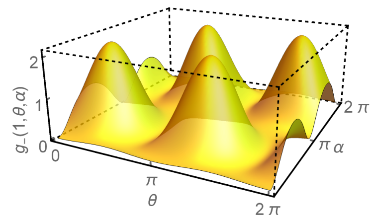
The latter can also be cast into
| (82a) | ||||
| with | ||||
| (82b) | ||||
| (82c) | ||||
| and | ||||
| (82d) | ||||
| Although the residue of Eq. (82a) does not look that involved, an analysis of this expression turned out to be challenging. Based on the new quantities of Eq. (82d), the modified DRs can be expressed in a short manner via | ||||
| (83) |
A further useful relation in this context is
| (84) |
According to our criterion, unitarity is guaranteed as long as . The second contribution of is manifestly nonnegative due to . However, the first is not. For the configurations and , the first term simply vanishes, i.e., unitarity can be demonstrated quickly for these special cases. In particular, the imaginary part of the residue for is
| (85) |
Specifically for the situation , DR (84) recovers the usual Maxwell DR and , so that the residue simply yields
| (86) |
The origin of the factor of 2 in the denominator is due to the existence of two distinct DRs for nonzero Lorentz violation and configurations other than . When both merge for vanishing Lorentz violation, each contributes the above value to the residue providing its standard result.


In contrast, for most other choices, an evaluation of the inequality seems to be highly involved. What can be done, is to employ observer rotational invariance and to choose a coordinate system such that the momentum points along the third axis and , lie in the plane spanned by the first and third axes. So we consider
| (87) |
with and . Inserting these representations into the left-hand side of , we obtain
| (88a) | ||||
| (88b) | ||||
| with | ||||
| (88c) | ||||
The left-hand side of the new inequality are functions of and the two angles , . It is challenging to prove that is nonnegative for general and angles. Plots of these functions for a given choice of are presented in Fig. 4. According to the plots, both functions most probably do not provide negative values. Numerical investigations allow for determining the zeros of ; cf. Fig. 5. There are no isolated zeros, but they lie along certain lines. Evaluating the first and second derivatives at these points, indicates that they are local minima. Minima other than those were not found. Hence, there are strong numerical indications that are nonnegative. Analog results can be obtained for , ensuring unitarity for such more general configurations of the purely spacelike case.
IV Conclusions and final remarks
We analyzed Maxwell’s electrodynamics modified by dimension-five and CPT-odd higher-derivative terms that are part of the photon sector of the nonminimal Standard-Model Extension. The first dimension-five term to be addressed was a kind of higher-derivative CFJ-like contribution. The propagator of the theory was computed by means of the algebra for the tensor operators involved. Based on this result, modifications of the properties of wave propagation due to the presence Lorentz violation were investigated.
The analysis of the dispersion relations obtained from the propagator poles revealed that signals do not propagate at all for the purely timelike sector. The modes of the purely spacelike sector decouple from the theory for low energies and only propagate in the high-energy regime. For this sector, classical causality is preserved for any choice of background coefficients. Furthermore, unitarity at tree-level was examined by contracting the propagator with conserved currents and studying the pole structure of the resulting expression. It was found that unitarity can be preserved in some special cases. In general, however, the dispersion relations describe nonunitary modes. This propagator possesses some analogy with that of MCFJ theory, which was shown in App. A. But the dispersion relations and the related physics of these two models differ from each other.
The second dimension-five term examined was an anisotropic higher-derivative CFJ-like contribution that can be identified with the photon sector of Myers-Pospelov theory. The propagator was again computed and the dispersion relations were obtained from it for a purely timelike and a purely spacelike background vector field. For the timelike background, one mode was found to be unphysical, whereas the second generally obeys classical causality and unitarity, as shown in Eq. (79). For the spacelike configuration, there are two modes, as well. One mode is causal when the propagation direction encloses an angle with the spacelike preferred direction and noncausal for complementary angles. The other mode is noncausal for all angles . However, numerical investigations indicate that unitarity is preserved for a large subset of configurations within this scenario (in spite of causality violation).
The results of this paper complement our findings for nonminimal CPT-even extensions of the electromagnetic sector considered in Leticia1. In general, the studies performed for the CPT-odd extensions were easier from a technical point of view in comparison to their CPT-even counterparts. Furthermore, our results reveal that a breakdown of classical causality does not necessarily imply unitarity violation at tree-level. Indeed, with regards to our results and those of Reyes:2013nca, we can safely conclude that the photon sector of Myers-Pospelov theory is well-behaved with respect to unitarity for a large number of parameter choices — at least based on the criteria studied in the current work and in Reyes:2013nca. This is the case even for the modes that violate causality. It is also known that a violation of classical causality does not always yield a violation of causality at the microscopic level, as was demonstrated for particular minimal models; cf. Klinkhamer:2010zs. Therefore, noncausal modes in this sense can still be of interest.
On the other hand, the fate of nonunitary modes is uncertain, as long as contributions of even higher mass dimensions that may cure this malign behavior are not taken into account. Another point connected with quantization and unitarity of this theory is how to suitably fix the gauge for addressing the additional degrees of freedom that usually appear in higher-derivative theories. Such cases can require a nonstandard gauge fixing condition. Another question to be tackled is if there is an analog of the Lee-Wick mechanism that allows us to preserve unitarity by decoupling the ghost modes and removing the negative-norm states from the asymptotic Hilbert space, even in the sectors plagued by nonunitarity behavior. One possibility of exploring this issue is to couple the higher-derivative electrodynamics to fermions and to use the optical theorem, as carried out in Ref. Reyes:2017pus.
CJF theory, which is CPT-odd and of dimension 3, is considered as a prototype Lorentz-violating modification of the photon sector that has been of great interest over the past 30 years. As its properties have already been studied in great detail, it was a natural step to look at its higher-dimensional versions of which the photon sector of Myers-Pospelov theory is one possible extension. We argued at the beginning that dimension-three modifications are suppressed for high energies, whereas the dimension-five terms studied here gain importance in this regime. The results of the paper indicate which sectors of the theory should be disregarded and which are suitable for quantization and phenomenological studies. Due to the arguments mentioned before, it may be worthwhile to consider modified particle-physics processes in the unitary sectors. An analysis of cosmic-ray data is likely to lead to an additional number of tight constraints on Lorentz violation that complement the already existing dimension-five photon sector bounds in the data tables KostRussell.
Acknowledgements.
The authors are grateful to CNPq, CAPES, and FAPEMA (Brazilian research agencies) for financial support. In particular, M.M. Ferreira is obliged to FAPEMA Universal 00880/15; FAPEMA PRONEX 01452/14; CNPq Produtividade 308933/2015-0. R.V. Maluf acknowledges CNPq Produtividade 307556/2018-2, and M. Schreck is thankful to FAPEMA Universal 01149/17; CNPq Universal 421566/2016-7; CNPq Produtividade 312201/2018-4. In addition, we thank Z. Li for pointing out the connection of our modifications with a subset of those compiled in NMkost2 and for helpful discussions. We are also indebted to the comments of the two anonymous referees that led to an improved discussion of the motivation of our work and the results obtained.Appendix A Comparison to propagator of MCFJ theory
It would be interesting to compare the propagator (20) with that of MCFJ theory, which will be carried out in the current section. The MCFJ Lagrange density is
| (89) |
where is the CFJ vector background and the last term is included to fix the gauge. Such a Lagrange density can be written as
| (90a) | ||||
| (90b) | ||||
with the projectors of Eq. (11). Using an algebra similar to that of Tab. 1, one obtains the following propagator:
| (91) |
with . In momentum space, the latter is
| (92a) | ||||
| (92b) | ||||
The replacement
| (93) |
implies
| (94a) | ||||
| (94b) | ||||
which, inserted into Eq. (92), leads to the propagator (20) of the first dimension-five model examined. Furthermore, this propagator, as it stands, corresponds to Eq. (3.3) of the first paper of Ref. Adam2 for , and , with an appropriate choice of the prefactor. Here, is the Chern-Simons mass and a fixed four-vector used in their axial gauge fixing condition.
Appendix B Mapping to the nonminimal SME
The modifications that we considered in this paper are as follows
| (95a) | ||||
| (95b) | ||||
with the vector-valued background fields and . We would like to map these Lagrangians onto those presented in NMkost2. As the related field operators are of mass dimension 5, the correct Lagrangian must be of their Tab. III with the observer tensor . The pieces antisymmetric in , and , contribute only. By performing a partial integration and neglecting the surface terms, can be brought into a form more suitable for us:
| (96) |
Comparing the latter to the previous Lagrange densities leads to the correspondences
| (97a) | ||||
| (97b) | ||||
for and , respectively. We see that both are symmetric in , due to the symmetry of the two spacetime derivatives. The problem is that the tensors are not antisymmetric in , . Hence, they should be antisymmetrized by hand. For example, for the first Lagrangian, we obtain
| (98) |
Inserting the latter into after performing the partial integration leads to
| (99) |
with the dual electromagnetic field strength tensor . The second contribution vanishes due to the homogenous Maxwell equations that are still valid in the presence of Lorentz violation. Hence, it is not necessary to antisymmetrize the tensors in , by hand, whereby the mappings of Eqs. (97) are valid as they stand. The same argument holds for the second modification.
References
- (1) D. Colladay and V.A. Kostelecký, Phys. Rev. D 55, 6760 (1997); D. Colladay and V.A. Kostelecký, Phys. Rev. D 58, 116002 (1998); S.R. Coleman and S.L. Glashow, Phys. Rev. D 59, 116008 (1999).
- (2) V.A. Kostelecký and S. Samuel, Phys. Rev. Lett. 63, 224 (1989); Phys. Rev. D 39, 683 (1989); Phys. Rev. D 40, 1886 (1989); Phys. Rev. Lett. 66, 1811 (1991); V.A. Kostelecký and R. Potting, Nucl. Phys. B 359, 545 (1991); Phys. Rev. D 51, 3923 (1995); Phys. Lett. B 381, 89 (1996).
- (3) O.W. Greenberg, Phys. Rev. Lett. 89, 231602 (2002).
- (4) V.A. Kostelecký and C.D. Lane, J. Math. Phys. 40, 6245 (1999); V.A. Kostelecký and R. Lehnert, Phys. Rev. D 63, 065008 (2001); D. Colladay and V.A. Kostelecký, Phys. Lett. B 511, 209 (2001); R. Lehnert, Phys. Rev. D 68, 085003 (2003); R. Lehnert, J. Math. Phys. 45, 3399 (2004); B. Altschul, Phys. Rev. D 70, 056005 (2004); G.M. Shore, Nucl. Phys. B 717, 86 (2005).
- (5) W.F. Chen and G. Kunstatter, Phys. Rev. D 62, 105029 (2000); O.G. Kharlanov and V.Ch. Zhukovsky, J. Math. Phys. 48, 092302 (2007); B. Gonçalves, Y.N. Obukhov, and I.L. Shapiro, Phys. Rev. D 80, 125034 (2009); S.I. Kruglov, Phys. Lett. B 718, 228 (2012); T.J. Yoder and G.S. Adkins, Phys. Rev. D 86, 116005 (2012); S. Aghababaei, M. Haghighat, and I. Motie, Phys. Rev. D 96, 115028 (2017).
- (6) B. Gonçalves, M.M. Dias Jr., and B.J. Ribeiro, Phys. Rev. D 99, 096015 (2019); Z. Xiao, Phys. Rev. D 94, 115020 (2016); Z. Xiao, Phys. Rev. D 93, 125022 (2016); Z. Xiao and B.-Q. Ma, Int. J. Mod. Phys. A 24, 1359 (2009).
- (7) R. Bluhm, V.A. Kostelecký, and N. Russell, Phys. Rev. Lett. 79, 1432 (1997); R. Bluhm, V.A. Kostelecký, and N. Russell, Phys. Rev. D 57, 3932 (1998); R. Bluhm, V.A. Kostelecký, and N. Russell, Phys. Rev. Lett. 82, 2254 (1999); V.A. Kostelecký and C.D. Lane, Phys. Rev. D 60, 116010 (1999); R. Bluhm and V.A. Kostelecký, Phys. Rev. Lett. 84, 1381 (2000); R. Bluhm, V.A. Kostelecký, and C.D. Lane, Phys. Rev. Lett. 84, 1098 (2000); R. Bluhm, V.A. Kostelecký, C.D. Lane, and N. Russell, Phys. Rev. Lett. 88, 090801 (2002).
- (8) S.M. Carroll, G.B. Field, and R. Jackiw, Phys. Rev. D 41, 1231 (1990); A.A. Andrianov and R. Soldati, Phys. Rev. D 51, 5961 (1995); A.A. Andrianov and R. Soldati, Phys. Lett. B 435, 449 (1998); A.A. Andrianov, R. Soldati, and L. Sorbo, Phys. Rev. D 59, 025002 (1998); J. Alfaro, A.A. Andrianov, M. Cambiaso, P. Giacconi, and R. Soldati, Int. J. Mod. Phys. A 25, 3271 (2010); A.A. Andrianov, D. Espriu, P. Giacconi, and R. Soldati, JHEP 0909, 057 (2009).
- (9) C. Adam and F.R. Klinkhamer, Nucl. Phys. B 607, 247 (2001); C. Adam and F.R. Klinkhamer, Nucl. Phys. B 657, 214 (2003); V.Ch. Zhukovsky, A.E. Lobanov, and E.M. Murchikova, Phys. Rev. D 73, 065016 (2006); Y.M.P. Gomes, P.C. Malta, Phys. Rev. D 94, 025031 (2016); A. Martín-Ruiz, C.A. Escobar, Phys. Rev. D 95, 036011 (2017).
- (10) A.P. Baêta Scarpelli, H. Belich, J.L. Boldo, and J.A. Helayël-Neto, Phys. Rev. D 67, 085021 (2003); R. Lehnert and R. Potting, Phys. Rev. Lett. 93, 110402 (2004); R. Lehnert and R. Potting, Phys. Rev. D 70, 125010 (2004); C. Kaufhold and F.R. Klinkhamer, Nucl. Phys. B 734, 1 (2006); B. Altschul, Phys. Rev. D 75, 105003 (2007); H. Belich, L.D. Bernald, P. Gaete, and J.A. Helayël-Neto, Eur. Phys. J. C 73, 2632 (2013).
- (11) B. Altschul, Phys. Rev. Lett. 98, 041603 (2007); C. Kaufhold and F.R. Klinkhamer, Phys. Rev. D 76, 025024 (2007); B. Altschul, Nucl. Phys. B 796, 262 (2008).
- (12) V.A. Kostelecký and M. Mewes, Phys. Rev. Lett. 87, 251304 (2001); V.A. Kostelecký and M. Mewes, Phys. Rev. D 66, 056005 (2002); V.A. Kostelecký and M. Mewes, Phys. Rev. Lett. 97, 140401 (2006); C.A. Escobar and M.A.G. Garcia, Phys. Rev. D 92, 025034 (2015); A. Martín-Ruiz and C.A. Escobar, Phys. Rev. D 94, 076010 (2016).
- (13) B. Altschul, Phys. Rev. Lett. 98, 041603 (2007); C. Kaufhold and F.R. Klinkhamer, Phys. Rev. D 76, 025024 (2007); F.R. Klinkhamer and M. Risse, Phys. Rev. D 77, 016002 (2008); F.R. Klinkhamer and M. Risse, Phys. Rev. D 77, 117901 (2008); F.R. Klinkhamer and M. Schreck, Phys. Rev. D 78, 085026 (2008).
- (14) A. Moyotl, H. Novales-Sanchez, J.J. Toscano, and E.S. Tututi, Int. J. Mod. Phys. A 29, 1450039 (2014); Int. J. Mod. Phys. A 29, 1450107 (2014).
- (15) M. Schreck, Phys. Rev. D 86, 065038 (2012); G. Gazzola, H.G. Fargnoli, A.P. Baêta Scarpelli, M. Sampaio, and M.C. Nemes, J. Phys. G 39, 035002 (2012); A.P. Baêta Scarpelli, J. Phys. G 39, 125001 (2012); B. Agostini, F.A. Barone, F.E. Barone, P. Gaete, and J.A. Helayël-Neto, Phys. Lett. B 708, 212 (2012); L.C.T. Brito, H.G. Fargnoli, and A.P. Baêta Scarpelli, Phys. Rev. D 87, 125023 (2013); S. Tizchang, R. Mohammadi, and S. Xue, Probing Lorentz violation effects via a laser beam interacting with a high-energy charged lepton beam, arXiv:1811.00486.
- (16) R. Jackiw and V.A. Kostelecký, Phys. Rev. Lett. 82, 3572 (1999); J.-M. Chung, Phys. Rev. D 60, 127901 (1999); M. Pérez-Victoria, Phys. Rev. Lett. 83, 2518 (1999); J.-M. Chung and B.K. Chung, Phys. Rev. D 63, 105015 (2001); G. Bonneau, Nucl. Phys. B 593, 398 (2001); M. Pérez-Victoria, JHEP 0104, 032 (2001).
- (17) O.A. Battistel and G. Dallabona, J. Phys. G 27, L53 (2001); Nucl. Phys. B 610, 316 (2001); A.P. Baêta Scarpelli, M. Sampaio, M.C. Nemes, and B. Hiller, Phys. Rev. D 64, 046013 (2001); O.A. Battistel and G. Dallabona, J. Phys. G 28, L23 (2002); B. Altschul, Phys. Rev. D 70, 101701(R) (2004); T. Mariz, J.R. Nascimento, E. Passos, R.F. Ribeiro, and F.A. Brito, JHEP 0510, 019 (2005); J.R. Nascimento, E. Passos, A.Yu. Petrov, and F.A. Brito, JHEP 0706, 016 (2007).
- (18) A.P. Baêta Scarpelli, M. Sampaio, M.C. Nemes, and B. Hiller, Eur. Phys. J. C 56, 571 (2008); F.A. Brito, J.R. Nascimento, E. Passos, and A.Yu. Petrov, Phys. Lett. B 664, 112 (2008); F.A. Brito, L.S. Grigorio, M.S. Guimaraes, E. Passos, and C. Wotzasek, Phys. Rev. D 78, 125023 (2008); O.M. Del Cima, J.M. Fonseca, D.H.T. Franco, and O. Piguet, Phys. Lett. B 688, 258 (2010).
- (19) V.A. Kostelecký and N. Russell, Rev. Mod. Phys. 83, 11 (2011).
- (20) V.A. Kostelecký and M. Mewes, Phys. Rev. D 80, 015020 (2009); M. Mewes, Phys. Rev. D 85, 116012 (2012); M. Schreck, Phys. Rev. D 89, 105019 (2014).
- (21) V.A. Kostelecký and M. Mewes, Phys. Rev. D 88, 096006 (2013); M. Schreck, Phys. Rev. D 90, 085025 (2014).
- (22) J.A.A.S. Reis and M. Schreck, Phys. Rev. D 95, 075016 (2017).
- (23) B. Podolsky, Phys. Rev. 62, 68 (1942); B. Podolsky and C. Kikuchi, Phys. Rev. 65, 228 (1944).
- (24) A. Accioly and E. Scatena, Mod. Phys. Lett. A 25, 269 (2010).
- (25) C.A.P. Galvão and B.M. Pimentel, Can. J. Phys. 66, 460 (1988).
- (26) R. Bufalo, B.M. Pimentel, and G.E.R. Zambrano, Phys. Rev. D 83, 045007 (2011); C.A. Bonin, R. Bufalo, B.M. Pimentel, and G.E.R. Zambrano, Phys. Rev. D 81, 025003 (2010).
- (27) R. Bufalo, B.M. Pimentel, and G.E.R. Zambrano, Phys. Rev. D 86, 125023 (2012); C.A. Bonin, B.M. Pimentel, and P.H. Ortega, Int. J. Mod. Phys. A 34, 1950134 (2019).
- (28) E.C. Manavella, Int. J. M. Phys. A 34, 1950050 (2019).
- (29) T.D. Lee and G.C. Wick, Nucl. Phys. B 9, 209 (1969); T.D. Lee and G.C. Wick, Phys. Rev D 2, 1033 (1970).
- (30) B. Grinstein and D. O’Connell, Phys. Rev. D 78, 105005 (2008); B. Grinstein, D. O’Connell, and M.B. Wise, Phys. Rev. D 77, 025012 (2008); J.R. Espinosa, B. Grinstein, D. O’Connell, and M.B. Wise, Phys. Rev. D 77, 085002 (2008); T.E.J. Underwood and R. Zwicky, Phys. Rev. D 79, 035016 (2009); R.S. Chivukula, A. Farzinnia, R. Foadi, and E.H. Simmons, Phys. Rev. D 82, 035015 (2010).
- (31) T.G. Rizzo, JHEP 0706, 070 (2007); T.G. Rizzo, JHEP 0801, 042 (2008); E. Álvarez, C. Schat, L. Da Rold, and A. Szynkman, JHEP 0804, 026 (2008); C.D. Carone and R. Primulando, Phys. Rev. D 80, 055020 (2009).
- (32) R. Turcati and M.J. Neves, Adv. High Energy Phys. 2014, 153953 (2014).
- (33) F.A. Barone, G. Flores-Hidalgo, and A.A. Nogueira, Phys. Rev. D 91, 027701 (2015).
- (34) A. Accioly, J. Helayël-Neto, F.E. Barone, F.A. Barone, and P. Gaete, Phys. Rev. D 90, 105029 (2014).
- (35) F.A. Barone, G. Flores-Hidalgo, and A.A. Nogueira, Phys. Rev. D 88, 105031 (2013).
- (36) F.A. Barone and A.A. Nogueira, Eur. Phys. J. C 75, 339 (2015).
- (37) D. Anselmi and M. Piva, JHEP 1706, 066 (2017); D. Anselmi and M. Piva, Phys. Rev. D 96, 045009 (2017).
- (38) R.C. Myers and M. Pospelov, Phys. Rev. Lett. 90, 211601 (2003); C.M. Reyes, L.F. Urrutia, and J.D. Vergara, Phys. Rev. D 78, 125011 (2008); J. Lopez-Sarrion and C.M. Reyes, Eur. Phys. J. C 72, 2150 (2012).
- (39) C.M. Reyes, L.F. Urrutia, and J.D. Vergara, Phys. Lett. B 675, 336 (2009).
- (40) C.M. Reyes, Phys. Rev. D 82, 125036 (2010).
- (41) C.M. Reyes, Phys. Rev. D 87, 125028 (2013).
- (42) E. Passos, E.M.C. Abreu, M.A. Anacleto, F.A. Brito, C. Wotzasek, and C.A.D. Zarro, Phys.Rev. D 93, 085022 (2016).
- (43) H. Belich, T. Costa-Soares, M.M. Ferreira, Jr., and J.A. Helayël-Neto, Eur. Phys. J. C 41, 421 (2005); H. Belich, L.P. Colatto, T. Costa-Soares, J.A. Helayël-Neto, and M.T.D. Orlando, Eur. Phys. J. C 62, 425 (2009); B. Charneski, M. Gomes, R.V. Maluf, and A.J. da Silva, Phys. Rev. D 86, 045003 (2012).
- (44) R. Casana, M.M. Ferreira, Jr., E. Passos, F.E.P. dos Santos, and E.O. Silva, Phys. Rev. D 87, 047701 (2013); J.B. Araujo, R. Casana, M.M. Ferreira, Jr., Phys. Rev. D 92, 025049 (2015); Phys. Lett. B 760, 302 (2016).
- (45) Y. Ding and V.A. Kostelecký, Phys. Rev. D 94, 056008 (2016).
- (46) V.A. Kostelecký and Z. Li, Phys. Rev. D 99, 056016 (2019).
- (47) Y.M.P. Gomes, J.T. Guaitolini Jr., Phys. Rev. D 99, 055006 (2019).
- (48) V.E. Mouchrek-Santos, M.M. Ferreira Jr., Phys. Rev. D 95, 071701(R) (2017).
- (49) V.E. Mouchrek-Santos, M.M. Ferreira Jr., and C. Miller, Nucl. Phys. B 945, 114677 (2019).
- (50) R. Casana, J.S. Rodrigues, and F.E.P. dos Santos, Phys. Lett. B 790, 354 (2019).
- (51) A.F. Santos, and Faqir C. Khanna, Phys. Rev. D 95, 125012 (2017); P.R.A. Souza, A.F. Santos, S.C. Ulhoa, and Faqir C. Khanna, Phys. Lett. B 791, 195 (2019); A.F. Santos and Faqir C. Khanna, Adv. High Energy Phys. 2018, 4596129 (2018).
- (52) S.M. Carroll, J.A. Harvey, V.A. Kostelecký, C.D. Lane, and T. Okamoto, Phys. Rev. Lett. 87, 141601 (2001).
- (53) L.H.C. Borges, A.G. Dias, A.F. Ferrari, J.R. Nascimento, and A.Yu. Petrov, Phys. Lett. B 756, 332 (2016); A.J.G.Carvalho, A.F.Ferrari, A.M.de Lima, J.R.Nascimento, and A.Yu.Petrov, Nucl. Phys. B 942, 393 (2019).
- (54) L.H.C. Borges, A.F. Ferrari, and F.A. Barone, Eur. Phys. J. C 76, 599 (2016);
- (55) L. Bonetti, L.R. dos Santos Filho, J.A. Helayël-Neto, and A.D.A.M. Spallicci, Phys. Lett. B 764, 203 (2017).
- (56) L. Bonetti, L.R. dos Santos Filho, J.A. Helayël-Neto, and A.D.A.M. Spallicci, Eur. Phys. J. C 78, 811 (2018).
- (57) M.A. Anacleto, F.A. Brito, E. Maciel, A. Mohammadi, E. Passos, W.O. Santos, and J.R.L. Santos, Phys. Lett. B 785, 191 (2018).
- (58) E. Passos, M.A. Anacleto, F.A. Brito, O. Holanda, G.B. Souza, and C.A.D. Zarro, Phys. Lett. B 772, 870 (2017).
- (59) K. Astapov, D. Kirpichnikov, and P. Satunin, JCAP04, 054 (2019); P. Satunin, New constraints on Lorentz invariance violation from Crab Nebula spectrum beyond 100 TeV, arXiv:1906.08221.
- (60) R. Casana, M.M. Ferreira, Jr., L. Lisboa-Santos, F.E.P. dos Santos, and M. Schreck, Phys. Rev. D 97, 115043 (2018).
- (61) A.P. Baêta Scarpelli, H. Belich, J.L. Boldo, and J.A. Helayël-Neto, Phys. Rev. D 67, 085021 (2003); R. Casana, M.M. Ferreira, Jr., A.R. Gomes, and F.E.P. dos Santos, Phys. Rev. D 82, 125006 (2010).
- (62) A. Moyotl, H. Novales-Sanchez, J.J. Toscano, and E.S. Tututi, Int. J. Mod. Phys. A 29, 1450107 (2014); T.R.S. Santos, R.F. Sobreiro, and A.A. Tomaz, Phys. Rev. D 94, 085027 (2016).
- (63) M.E. Peskin and D.V. Schroeder, An Introduction to Quantum Field Theory (Perseus Books Publishing, L.L.C., Reading; Massachusetts, 1995).
- (64) V.A. Kostelecký and N. Russell, Phys. Lett. B 693, 443 (2010); V.A. Kostelecký, Phys. Lett. B 701, 137 (2011); J. Foster and R. Lehnert, Phys. Lett. B 746, 164 (2015).
- (65) R.V. Maluf, C.A.S. Almeida, R. Casana, and M.M. Ferreira Jr., Phys. Rev. D 90, 025007 (2014).
- (66) R.V. Maluf, A.A. Araújo Filho, W.T. Cruz, and C.A.S. Almeida, EPL 124, 61001 (2018).
- (67) K.J. Barnes, Ph.D. thesis, University of London, 1963 (unpublished).
- (68) R.J. Rivers, Nuovo Cim. 34, 386 (1964).
- (69) E. Sezgin, P. van Nieuwenhuizen, Phys. Rev. D 21, 3269 (1980).
- (70) L. Brillouin, Wave propagation and group velocity (Academic Press, New York and London, 1960).
- (71) M. Veltman, in Methods in Field Theory, edited by R. Balian and J. Zinn-Justin (World Scientific, Singapore, 1981).
- (72) F.R. Klinkhamer and M. Schreck, Nucl. Phys. B 848, 90 (2011).
- (73) C.M. Reyes and L.F. Urrutia, Phys. Rev. D 95, 015024 (2017); M. Maniatis and C.M. Reyes, Phys. Rev. D 89, 056009 (2014).