DNA: Deeply-supervised Nonlinear Aggregation for Salient Object Detection

Yun Liu Ming-Ming Cheng Xin-Yu Zhang Guang-Yu Nie and Meng Wang Thanks: Manuscript received April 19, 2005; revised August 26, 2015. Major Project for New Generation of AI under Grant No. 2018AAA0100400, NSFC (NO. 61620106008), S&T innovation project from Chinese Ministry of Education, and Tianjin Natural Science Foundation for Distinguished Young Scholars (NO. 17JCJQJC43700). Thanks: Y. Liu, M.-M. Cheng, and X.-Y. Zhang are with Nankai University. M.-M. Cheng (cmm@nankai.edu.cn) is the corresponding author. Thanks: G.-Y. Nie is with Beijing Institute of Technology. Thanks: M. Wang is with Hefei University of Technology.

Abstract

Recent progress on salient object detection mainly aims at exploiting how to effectively integrate multi-scale convolutional features in convolutional neural networks (CNNs). Many popular methods impose deep supervision to perform side-output predictions that are linearly aggregated for final saliency prediction. In this paper, we theoretically and experimentally demonstrate that linear aggregation of side-output predictions is suboptimal, and it only makes limited use of the side-output information obtained by deep supervision. To solve this problem, we propose Deeply-supervised Nonlinear Aggregation (DNA) for better leveraging the complementary information of various side-outputs. Compared with existing methods, it i) aggregates side-output features rather than predictions, and ii) adopts nonlinear instead of linear transformations. Experiments demonstrate that DNA can successfully break through the bottleneck of current linear approaches. Specifically, the proposed saliency detector, a modified U-Net architecture with DNA, performs favorably against state-of-the-art methods on various datasets and evaluation metrics without bells and whistles.

Index Terms:

Salient object detection, saliency detection, deeply-supervised nonlinear aggregation.

I Introduction

Salient object detection, also known as saliency detection, aims at simulating the human vision system to detect the most conspicuous and eye-attracting objects or regions in natural images [1, 2, 3]. The progress in saliency detection has been beneficial to a wide range of vision applications, including image retrieval [4, 5], visual tracking [6], scene classification [7], content-aware image/video processing [8, 9], thumbnail generation [10], video object segmentation [11], and weakly supervised learning [12, 13]. Although numerous models have been presented [14, 15, 16, 17, 18, 19, 20, 21, 22, 23] and significant improvement has been made, it still remains an open problem to accurately detect complete salient objects in static images, especially in complicated scenarios.

\begin{overpic}[frame_comp3] \put(12.5,0.4){\footnotesize\cite[cite]{[\@@bibref{}{hariharan2015hypercolumns}{}{}]}} \put(26.7,0.4){\footnotesize\cite[cite]{[\@@bibref{}{ronneberger2015u}{}{}]}} \put(42.2,0.4){\footnotesize\cite[cite]{[\@@bibref{}{xie2017holistically}{}{}]}} \put(57.8,0.4){\footnotesize\cite[cite]{[\@@bibref{}{ronneberger2015u}{}{}]}} \put(65.6,0.4){\footnotesize\cite[cite]{[\@@bibref{}{xie2017holistically}{}{}]}} \end{overpic}

Fig. 1: Illustration of different multi-scale deep learning architectures. Note that (c)-(e) use deep supervision to produce side-outputs, but (c) and (d) linearly aggregate side-output predictions, while the proposed DNA (e) adopts nonlinear aggregation onto side-output features.

Conventional saliency detection methods [2, 27, 28] usually design hand-crafted low-level features and heuristic priors, which are difficult to represent semantic objects and scenes. Recent advances on saliency detection mainly benefit from convolutional neural networks (CNNs) [29, 30, 31, 32, 33]. On the one hand, CNNs naturally learn multi-scale and multi-level feature representations in each layer due to the increasingly larger receptive fields and downsampled (strided) scales [34]. On the other hand, salient object detection requires multi-scale learning because of the various object/scene scales in intra- and inter-images [35, 36]. Therefore, current cutting-edge saliency detectors [15, 37, 38, 39, 17, 40, 41, 42, 43] mainly aim at designing complex network architectures to leverage multi-scale CNN features, e.g., the semantic meaningful information in the top sides and the complementary spatial details in the bottom sides.

Owing to the superiority of U-Net [25] (or FCN [44]) and HED [26] in multi-scale learning, many leading-edge saliency detectors add deep supervision onto U-Net networks [16, 38, 17, 18, 41, 45, 19], [46] (Fig. 1(d)). We note that these networks first predict multi-scale saliency maps using side-outputs. The generated multi-scale side-output predictions are then linearly aggregated, e.g., via a pixel-wise convolution (i.e., $1\times 1$ convolution), to obtain the final saliency prediction which can thus combine the advantages of all side-output predictions. However, we theoretically and experimentally demonstrate that the linear aggregation of side-output predictions is suboptimal, and it makes limited use of the complementary multi-scale information implicated in side-output features. We provide detailed proofs in Section III.

Instead of linearly aggregating side-output predictions, we propose a nonlinear side-output aggregation method. Specifically, we concatenate the side-output features rather than side-output predictions and then apply nonlinear transformations to predict salient objects. We also impose deep supervision to side-output features for better optimization in the training phase, as illustrated in Fig. 1(e). In this way, the concatenated features can make better use of the multi-scale side-output features. We call the resulting method Deeply-supervised Nonlinear Aggregation (DNA). We apply DNA into a simply redesigned U-Net without bells and whistles. The proposed network performs favorably against all previous state-of-the-art salient object detectors with less parameters and faster speed. Our contributions are twofold:

•

We theoretically and experimentally analyze the natural limitation of traditional linear side-output aggregation which can only make limited use of multi-scale side-output information.
•

We propose Deeply-supervised Nonlinear Aggregation (DNA) for side-output features, whose effectiveness has been proved by introducing it into a simple network with less parameters and faster speed.

II Related Work

Salient object detection is a very active research field due to its wide range of applications and challenging scenarios. Early heuristic saliency detection methods extract hand-crafted low-level features and apply machine learning models to classify these features [47, 48, 49]. Some heuristic saliency priors are utilized to ensure the accuracy, such as color contrast [1, 2], center prior [50, 27] and background prior [51, 52]. With vast successes achieved by deep CNNs in computer vision, CNN-based methods have been introduced to improve saliency detection [53, 54, 55, 56, 57]. Region-based saliency detection [58, 59, 60, 61, 62, 20, 21] appeared in the early era of deep learning based saliency. These approaches view each image patch as a basic processing unit to perform saliency detection. More recently, CNN-based image-to-image saliency detection [15, 16, 37, 38, 39, 17, 40, 18, 41, 63, 42, 64, 65, 43, 66, 67, 45, 22, 23] has dominated this field by viewing saliency detection as a pixel-wise regression task and performing image-to-image predictions. Hence we mainly review CNN-based image-to-image saliency detection in the following.

Since saliency detection requires both high-level global information (existing in the top sides of CNNs) and low-level local details (existing in the bottom sides of CNNs), how to effectively fuse multi-level deep features is the main research direction [15, 37, 38, 39, 17, 40, 41, 42, 43, 66, 67, 45, 68, 69]. There are too many studies to list here, but the general trend of recent network designs is to become more and more complicated. We continue our discussion by briefly categorizing multi-scale deep learning into four classes: hyper feature learning, U-Net style, HED style, and U-Net + HED style. An overall illustration of them is shown in Fig. 1.

Hyper feature learning: Hyper feature learning [24, 70, 71] is the most intuitive way to learn multi-scale information, as illustrated in Fig. 1(a). Examples of this structure for saliency include [66, 37, 63, 42, 64, 72, 65, 73]. These models concatenate/sum multi-scale deep features from multiple layers of backbone nets [66, 37] or branches of the multi-stream nets [63, 42, 64]. The fused hyper features, called hypercolumn, are then used for final predictions.

U-Net style: It is widely accepted that the top layers of deep neural networks contain high-level semantic information, while the bottom layers learn low-level fine details. Therefore, a reasonable revision of hyper feature learning is to progressively fuse deep features from upper layers to lower layers [44, 25], as shown in Fig. 1(b). The top semantic features will combine with bottom low-level features to capture fine-grained details. The feature fusion can be a simple element-wise summation [44], a simple feature map concatenation (U-Net) [25], or complex designs based on them. Many saliency detectors are of this type [74, 75, 67, 76, 40, 39, 14, 77, 78]. Note that hyper feature learning and U-Net do not apply deep supervision, so they do not have side-outputs.

HED style: HED-like networks [26, 79, 80] were first presented for edge detection. Afterwards, similar ideas have been also introduced for saliency detection [15, 43]. HED-like networks add deep supervision at the intermediate sides to obtain side-output predictions, and the final result is a linear combination of all side-output predictions (shown in Fig. 1(c)). Unlike multi-scale feature fusion, HED performs multi-scale prediction fusion.

U-Net + HED style: These methods combine the advantages of both U-Net and HED. We outline this architectures in Fig. 1(d). Specifically, deep supervision is imposed at each of the convolution stage of U-Net decoder. Many recent saliency models fall into this category [16, 38, 17, 18, 41, 81, 45, 19, 82, 83, 84, 85, 23], [46]. They differ from each other by applying different fusion strategies. One notable similarity of these models is that the final prediction is produced by a linear aggregation of side-output predictions. Hence the multi-scale learning is achieved in two aspects: i) the U-Net aggregates multi-level convolutional features from top layers to bottom layers in an encoder-decoder form; ii) the multi-scale side-output predictions are further linearly aggregated for final prediction. Current research in this field mainly focuses on the first aspect, and top-performing models have designed very complex feature fusion strategies for this [17, 41].

A full literature review of salient object detection is beyond the scope of this paper. Please refer to [86, 87, 88] for more comprehensive surveys. In this paper, we focus on the second aspect of above U-Net + HED multi-scale learning: the multi-scale side-output aggregation. We find that the upper bound of traditional linear side-output prediction aggregation is limited to the side-output predictions. Hence we propose DNA to aggregate side-output features in the nonlinear way, so that the aggregated hybrid features can make good use of the complementary multi-scale deep features. A streamlined diagram of our proposed DNA can be seen in Fig. 1(e). We demonstrate DNA can achieve superior performance with a very simple U-Net.

III Revisiting Linear Side-output Aggregation

Deep supervision and corresponding linear side-output prediction aggregation have been demonstrated to be effective in many vision tasks [26, 79, 17, 41]. This section analyzes the natural limitation of the linear side-output aggregation from both theoretical and experimental perspectives. To the best of our knowledge, this is a novel contribution.

Suppose a deeply-supervised network has $N$ side-output prediction maps $\{\mathcal{O}_{1},\mathcal{O}_{2},\cdots,\mathcal{O}_{N}\}$ , all of which are supervised by ground-truth maps (Fig. 1(c)(d)). Without loss of generality, we assume the linear side-output aggregation is a pixel-wise convolution, i.e., $1\times 1$ convolution. Hence, current linear side-output aggregation can be written as

\widehat{\mathcal{O}}=\sum_{i=1}^{N}\bm{w}_{i}\cdot\mathcal{O}_{i},

(1)

where weights $\bm{w}_{i}$ of pixel-wise convolution can be learned. Note that we have $\bm{w}_{i}\geq 0$ here. Otherwise, $\mathcal{O}_{i}$ would have negative effect to $\widehat{\mathcal{O}}$ , so it should be excluded in the aggregation. To obtain the output saliency probability map, a standard sigmoid function $\sigma(x)=\frac{1}{1+e^{-x}}$ should be applied to $\widehat{\mathcal{O}}$ . The aggregated probability map becomes

\widehat{\mathcal{P}}=\sigma(\widehat{\mathcal{O}})=\sigma(\sum_{i=1}^{N}\bm{w}_{i}\cdot\mathcal{O}_{i}).

(2)

Similarly, we can compute side-output probability maps $\{\mathcal{P}_{1},\mathcal{P}_{2},\cdots,\mathcal{P}_{N}\}$ .

Theorem 1.

If $\|\bm{w}\|_{1}=1$ , the mean absolute error (MAE) of fused output $\widehat{\mathcal{P}}$ is limited by side-output predictions.

Proof.

If $\|\bm{w}\|_{1}=1$ , it is natural to show

\min(\mathcal{O}_{i})\leq\sum_{i=1}^{N}\bm{w}_{i}\cdot\mathcal{O}_{i}\leq\max(\mathcal{O}_{i}),

(3)

because $\bm{w}_{i}\geq 0$ as discussed above. Since the sigmoid function $\sigma(x)$ is monotonically increasing, we have

\min(\mathcal{P}_{i})\leq\widehat{\mathcal{P}}\leq\max(\mathcal{P}_{i}).

(4)

If a pixel $\bm{p}$ is positive, we have $\text{MAE}(\widehat{\mathcal{P}})_{\bm{p}}=|1-\widehat{\mathcal{P}}(\bm{p})|=1-\widehat{\mathcal{P}}(\bm{p})$ and $1-\max(\mathcal{P}_{i})_{\bm{p}}\leq 1-\widehat{\mathcal{P}}(\bm{p})\leq 1-\min(\mathcal{P}_{i})_{\bm{p}}$ , so that $\min(\text{MAE}(\mathcal{P}_{i})_{\bm{p}})\leq\text{MAE}(\widehat{\mathcal{P}})_{\bm{p}}\leq\max(\text{MAE}(\mathcal{P}_{i})_{\bm{p}})$ holds. If the pixel $\bm{p}$ is negative, we have $\text{MAE}(\widehat{\mathcal{P}})_{\bm{p}}=|0-\widehat{\mathcal{P}}(\bm{p})|=\widehat{\mathcal{P}}(\bm{p})$ and $\min(\mathcal{P}_{i})_{\bm{p}}\leq\widehat{\mathcal{P}}(\bm{p})\leq\max(\mathcal{P}_{i})_{\bm{p}}$ , so that $\min(\text{MAE}(\mathcal{P}_{i})_{\bm{p}})\leq\text{MAE}(\widehat{\mathcal{P}})_{\bm{p}}\leq\max(\text{MAE}(\mathcal{P}_{i})_{\bm{p}})$ holds. Note that $\bm{w}$ usually only has $N$ ( $N\leq 6$ in VGG16 [89] and ResNet [90]) dimensions, so it is also difficult to make aforementioned left equality hold. Hence traditional linear aggregation is limited in terms of MAE metric. However, what we expect is to break through the limitation by making full use of multi-scale information. ∎

Lemma 1.

If $\|\bm{w}\|_{1}\neq 1$ , traditional linear aggregation (as in Eq. (1) and Eq. (2)) is equivalent to first applying an aggregation with $\|\bm{\tilde{w}}\|_{1}=1$ and then applying a monotonically increasing mapping.

Proof.

If $\|\bm{w}\|_{1}\neq 1$ , we set $\bm{w}=\bm{\tilde{w}}\cdot\|\bm{w}\|_{1}$ , so we have $\|\bm{\tilde{w}}\|_{1}=1$ . The computation of $\widehat{\mathcal{P}}$ becomes

\widehat{\mathcal{P}}=\sigma(\|\bm{w}\|_{1}\cdot\sum_{i=1}^{N}\bm{\tilde{w}}_{i}\cdot\mathcal{O}_{i}),

(5)

in which $\sigma(\|\bm{w}\|_{1}\cdot x)$ $(\|\bm{w}\|_{1}>0)$ is a monotonically increasing function in terms of $x$ . ∎

Refer to caption — Fig. 2: Probability ( $x$ axis) *vs.* the density of $X^{\prime}$ and $Y^{\prime}$ ( $y$ axis). TN: true negative; FN: false negative; TP: true positive; FP: false positive.

Theorem 2.

The monotonically increasing mapping of $\sigma(\|\bm{w}\|_{1}\cdot x)$ $(\|\bm{w}\|_{1}>0)$ cannot change the ROC curve and AUC metric¹¹ 1 AUC is the area under the ROC Curve..

Proof.

Suppose the predicted scores of positive samples obey the distribution of $X\sim F(x)$ , while the predicted scores of negative samples obey the distribution of $Y\sim G(x)$ . We may assume $F$ and $G$ are continuous functions. $\varphi(x)=\sigma(k\cdot x)$ $(k>0)$ is a variant of sigmoid function, so we have $\varphi:\mathbb{R}\to(0,1)$ and $\varphi$ is a monotonically increasing function. Let $X^{\prime}=\varphi(X)$ and $Y^{\prime}=\varphi(Y)$ be two transformed distributions. It is easy to show

	$\displaystyle\mathbb{P}(X^{\prime}\leq u)=\mathbb{P}(\varphi(X)\leq u)$	$\displaystyle=\mathbb{P}(X\leq\varphi^{-1}(u))$		(6)
		$\displaystyle=F(\varphi^{-1}(u)),$		(6)

and thus we can obtain $X^{\prime}\sim F(\varphi^{-1}(x))$ and $Y^{\prime}\sim G(\varphi^{-1}(x))$ .

TABLE I: Comparison between linear side-output prediction aggregation (i.e., lin) and nonlinear side-output feature aggregation (i.e., nonlin). The datasets and metrics will be introduced in Section V-A. The linear aggregation of HED [26] and DSS [43] follows the original papers, and their nonlinear aggregation replaces linear aggregation with the proposed DNA.

Methods	Fusion	DUTS-TE		ECSSD		HKU-IS		DUT-O		THUR15K
Methods	Fusion	$F_{\beta}$	MAE	$F_{\beta}$	MAE	$F_{\beta}$	MAE	$F_{\beta}$	MAE	$F_{\beta}$	MAE
HED [26]	linear	0.796	0.079	0.892	0.065	0.893	0.052	0.726	0.100	0.757	0.099
HED [26]	nonlinear	0.827	0.057	0.911	0.053	0.912	0.039	0.752	0.078	0.775	0.083
DSS [43]	linear	0.827	0.056	0.915	0.056	0.913	0.041	0.774	0.066	0.770	0.074
DSS [43]	nonlinear	0.833	0.055	0.918	0.056	0.916	0.040	0.784	0.060	0.773	0.072
DNA	linear	0.844	0.048	0.921	0.050	0.917	0.034	0.765	0.066	0.785	0.071
DNA	nonlinear	0.865	0.044	0.935	0.041	0.930	0.031	0.799	0.056	0.793	0.069

Let $t$ be a threshold, true positive rate (TPR) and false positive rate (FPR) can be computed as

	$\displaystyle\text{TPR}=\frac{\text{TP}}{\text{TP}+\text{FN}}=\mathbb{P}(X^{\prime}>t)=1-F(\varphi^{-1}(t)),$		(7)
	$\displaystyle\text{FPR}=\frac{\text{FP}}{\text{FP}+\text{TN}}=\mathbb{P}(Y^{\prime}>t)=1-G(\varphi^{-1}(t)),$		(7)

as shown in Fig. 2. Hence we can denote the ROC curve as $\{(1-F(\varphi^{-1}(t)),1-G(\varphi^{-1}(t))):t\in(0,1)\}$ . It is easy to show that as $t$ goes from $0$ to $1$ continuously, $(1-F(\varphi^{-1}(t)),1-G(\varphi^{-1}(t)))$ will change from $(1,1)$ to $(0,0)$ continuously and monotonically. It is also obvious to see that $\{(1-F(\varphi^{-1}(t)),1-G(\varphi^{-1}(t)))\}$ and $\{(F(\varphi^{-1}(t)),G(\varphi^{-1}(t)))\}$ are symmetric about the point $(\frac{1}{2},\frac{1}{2})$ . Suppose the area under the curve $\{(1-F(\varphi^{-1}(t)),1-G(\varphi^{-1}(t)))\}$ is $S_{1}$ , and the area under the curve $\{(F(\varphi^{-1}(t)),G(\varphi^{-1}(t)))\}$ is $S_{2}$ . By symmetry, we have $S_{1}+S_{2}=1$ .

With the above conclusions, we can compute $S_{2}$ as

	$\displaystyle S_{2}$	$\displaystyle=\int_{0}^{1}G(\varphi^{-1}(t))dF(\varphi^{-1}(t))$		(8)
		$\displaystyle=\int_{-\infty}^{+\infty}G(x)dF(x).$		(8)

Therefore, $S_{2}$ is independent of the specific form of the function $\varphi(x)$ , and $S_{1}=1-S_{2}$ is independent of $\varphi(x)$ , too. Moreover, as $t$ ranges in $(0,1)$ , thus $\varphi^{-1}(t)$ ranges in $\mathbb{R}$ . We have

		$\displaystyle\{(1-F(\varphi^{-1}(t)),1-G(\varphi^{-1}(t))):t\in(0,1)\}$		(9)
		$\displaystyle=\{(1-F(x),1-G(x)):x\in\mathbb{R}\},$		(9)

which is also independent of the form of $\varphi(x)$ . When $F(x)$ and $G(x)$ are discrete, the set $\{(1-F(\varphi^{-1}(t)),1-G(\varphi^{-1}(t))):t\in(0,1)\}$ is discrete but still independent of $\varphi(x)$ . Therefore, we can conclude that $\varphi(x)$ cannot change the ROC curve and AUC metric. ∎

Similar to the proof for Theorem 1, we can easily demonstrate that the first step in Lemma 1, i.e., linear aggregation with $\|\bm{\tilde{w}}\|_{1}=1$ , has limited MAE results. From Theorem 2, we know the second step in Lemma 1, i.e., a monotonically increasing mapping, cannot change the ROC curve and AUC value. Therefore, we can conclude that traditional linear aggregation with $\|\bm{w}\|_{1}\neq 1$ has limited improvement. Combined with Theorem 1, we can conclude that linear aggregation of side-outputs only has limited improvement.

Besides the theoretical proofs, we also perform experiments to compare linear aggregation versus nonlinear aggregation for salient object detection. To this end, we use the proposed nonlinear side-output feature aggregation (in Section IV-B) for nonlinear regression to evaluate two well-known models: HED [26] and DSS [43], and the proposed DNA model. The results are summarized in Table I. We can see significant improvement from linear regression to nonlinear regression. Based on this observation, this paper aims at designing a simple network with nonlinear side-output aggregation for effective salient object detection.

IV Methodology

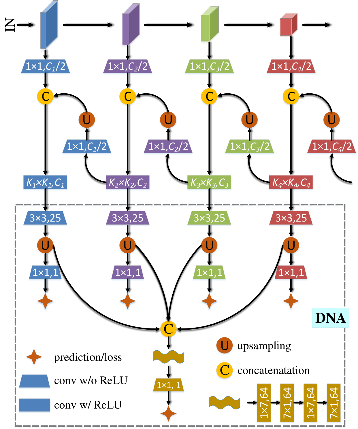
In this section, we will elaborate our proposed framework for salient object detection. We first introduce our base network in Section IV-A. Then, we present the deeply-supervised nonlinear aggregation in Section IV-B. An overall network architecture is illustrated in Fig. 3.

IV-A Base Network

Backbone network. To tackle the salient object detection, we follow recent studies [63, 42, 43] to use fully convolutional networks. Specifically, we use the well-known VGG16 network [89] as our backbone network, whose final fully connected layers are removed to serve for image-to-image translation. Salient object detection usually requires global information to locate the coarse positions of salient objects [2], so enlarging the receptive field of the network would be helpful. To this end, we keep the final pooling layer of VGG16 as in [43] and replace the last two fully connected layers with two convolution layers, one of which has the kernel size of $3\times 3$ with $C_{6}^{(1)}=192$ channels and another of which has the kernel size of $7\times 7$ with $C_{6}^{(2)}=128$ channels. Here, we use the $3\times 3$ convolution layer to reduce the feature channels, because large kernel sizes (e.g., $7\times 7$ ) lead to much more parameters.

There are five pooling layers in the backbone network. They divide the convolution layers into six convolution blocks, which are denoted as $\{\mathcal{S}^{1},\mathcal{S}^{2},\mathcal{S}^{3},\mathcal{S}^{4},\mathcal{S}^{5},\mathcal{S}^{6}\}$ from bottom to top, respectively. We consider $\mathcal{S}^{6}$ as the top valve that controls the overall contextual information that flows in the network. The resolution of the feature maps in each convolution block is half of the preceding one. Following [43, 26], the side-output of each convolution block is connected from the last layer of this block.

Encoder-decoder network. Based on the backbone net, we build an encoder-decoder network that can be seen in Fig. 3. Concretely, we connect a $1\times 1$ convolution layer to each of the convolution blocks $\mathcal{S}^{6}$ and $\mathcal{S}^{5}$ to adjust the number of channels (as shown in Table II). Then, we upsample the obtained feature maps from $\mathcal{S}^{6}$ by two. The upsampled feature maps and resulting feature maps from $\mathcal{S}^{5}$ are concatenated. To fuse the concatenated feature maps, two sequential convolution layers are used to generate the decoder side $\widetilde{\mathcal{S}}^{5}$ . The decoder sides $\{\widetilde{\mathcal{S}}^{4},\widetilde{\mathcal{S}}^{3},\widetilde{\mathcal{S}}^{2},\widetilde{\mathcal{S}}^{1}\}$ can be obtained in the same manner. For a clear presentation, we formulate the above process as follows

$\displaystyle\widetilde{\mathcal{S}}^{i}$	$\displaystyle=\varphi({\rm Concat}(\phi_{1}(\mathcal{S}^{i}),\phi_{2}(\widetilde{\mathcal{S}}^{i+1}))),$	(10)
$\displaystyle\phi_{1}(\cdot)$	$\displaystyle={\rm Conv}(\cdot),$
$\displaystyle\phi_{2}(\cdot)$	$\displaystyle={\rm Upsample}({\rm Conv}(\cdot)),$
$\displaystyle\varphi(\cdot)$	$\displaystyle={\rm ReLU}({\rm Conv}(\cdot)),$
$\displaystyle\forall i$	$\displaystyle\in\{1,2,3,4,5\}.$

Note that we have $\widetilde{\mathcal{S}}^{6}=\mathcal{S}^{6}$ , because $\mathcal{S}^{6}$ is the last block in the encoder path and also the first block in the decoder path. In this way, the proposed encoder-decoder lets top contextual information flow into the lower layers, so the lower layers are expected to emphasize the details of salient objects in an image. Here, both two sequential convolution layers ( $\varphi(\cdot)$ ) at the decoder side $\widetilde{\mathcal{S}}^{i}$ are with kernel size of $K_{i}\times K_{i}$ and output channels of $C_{i}$ . We will discuss the parameter settings in detail in the experiment part.

TABLE II: Network configurations.

Side	$C_{i}$	$K_{i}\times K_{i}$	Resolution
Side-output 1	64	$3\times 3$	1
Side-output 2	128	$3\times 3$	1/2
Side-output 3	128	$5\times 5$	1/4
Side-output 4	128	$5\times 5$	1/8
Side-output 5	128	$5\times 5$	1/16
Side output 6	-	-	1/32

IV-B Deeply-supervised Nonlinear Aggregation

Instead of linearly aggregating side-output predictions at multiple sides as in previous literature [16, 38, 17, 18, 41, 45, 19], we propose to aggregate the side-output features in a nonlinear way. The proposed DNA module is displayed in the dotted box of Fig. 3. Specifically, we first adopt a $3\times 3$ convolution for each $\widetilde{\mathcal{S}}^{i}$ to adjust the number of channels. Then, the feature maps are upsampled into the same size of the original image to generate side-output features. The side-output features can predict saliency maps using a simple $1\times 1$ convolution. In the training phase, deep supervision is added for these predicted maps.

We concatenate all side-output features to construct hybrid features that contain rich multi-scale and multi-level information. One of the key ideas in our nonlinear aggregation is that we use asymmetric convolution that decomposes a standard two-dimensional convolution into two one-dimensional convolutions. That is to say, a $n\times n$ convolution is decomposed into two sequential convolutions with kernel sizes of $1\times n$ and $n\times 1$ . Here, the reasons why we use asymmetric convolution are twofold. On one hand, in the experiments, we find large kernel size in the DNA module can improve performance, and we believe it is because hybrid feature maps have large resolution, i.e., the same resolution as the original image. On the other hand, convolutions with large kernel sizes are very time-consuming for large feature maps. According to the above analyses, we set $n=7$ for asymmetric convolutions rather than small kernel sizes. Larger kennel sizes than $n=7$ will only lead to little accuracy improvement while causing more computational load. The effectiveness of this choice has been validated in Section V-C where we try different settings of $n$ and asymmetric/standard convolutions. We use two groups of asymmetric convolutions, each of which consists of a $1\times 7$ and a $7\times 1$ convolution. With a $300\times 300$ input image, the number of FLOPs (multiply-adds) for these asymmetric convolutions is 13.8G, while the number of FLOPs will be 60.4G if we use the standard two-dimensional $7\times 7$ convolutions. At last, we connect a $1\times 1$ convolution after the asymmetric convolutions to predict the final saliency maps.

TABLE III: Comparison between the proposed DNA and 16 competitors in terms of the metrics of

F_{\beta}

and MAE on six datasets. We report results on both VGG16 [89] backbone and ResNet-50 [90] backbone. The top three models in each column are highlighted in red, green and blue, respectively. For ResNet-50 based methods, we only highlight the top performance.

Methods	DUTS-TE		ECSSD		HKU-IS		DUT-O		SOD		THUR15K
Methods	$F_{\beta}$	MAE	$F_{\beta}$	MAE	$F_{\beta}$	MAE	$F_{\beta}$	MAE	$F_{\beta}$	MAE	$F_{\beta}$	MAE
Non-deep learning
DRFI [27]	0.649	0.154	0.777	0.161	0.774	0.146	0.652	0.138	0.704	0.217	0.670	0.150
VGG16 [89] backbone
MDF [60]	0.707	0.114	0.807	0.138	-	-	0.680	0.115	0.764	0.182	0.669	0.128
LEGS [59]	0.652	0.137	0.830	0.118	0.766	0.119	0.668	0.134	0.733	0.194	0.663	0.126
DCL [66]	0.785	0.082	0.895	0.080	0.892	0.063	0.733	0.095	0.831	0.131	0.747	0.096
DHS [45]	0.807	0.066	0.903	0.062	0.889	0.053	-	-	0.822	0.128	0.752	0.082
ELD [61]	0.727	0.092	0.866	0.081	0.837	0.074	0.700	0.092	0.758	0.154	0.726	0.095
RFCN [74]	0.782	0.089	0.896	0.097	0.892	0.080	0.738	0.095	0.802	0.161	0.754	0.100
NLDF [67]	0.806	0.065	0.902	0.066	0.902	0.048	0.753	0.080	0.837	0.123	0.762	0.080
DSS [43]	0.827	0.056	0.915	0.056	0.913	0.041	0.774	0.066	0.842	0.122	0.770	0.074
Amulet [41]	0.778	0.085	0.913	0.061	0.897	0.051	0.743	0.098	0.795	0.144	0.755	0.094
UCF [75]	0.772	0.112	0.901	0.071	0.888	0.062	0.730	0.120	0.805	0.148	0.758	0.112
PiCA [17]	0.837	0.054	0.923	0.049	0.916	0.042	0.766	0.068	0.836	0.102	0.783	0.083
C2S [14]	0.811	0.062	0.907	0.057	0.898	0.046	0.759	0.072	0.819	0.122	0.775	0.083
RAS [15]	0.831	0.059	0.916	0.058	0.913	0.045	0.785	0.063	0.847	0.123	0.772	0.075
DNA	0.865	0.044	0.935	0.041	0.930	0.031	0.799	0.056	0.853	0.107	0.793	0.069
ResNet-50 [90] backbone
SRM [42]	0.826	0.059	0.914	0.056	0.906	0.046	0.769	0.069	0.840	0.126	0.778	0.077
BRN [40]	0.827	0.050	0.919	0.043	0.910	0.036	0.774	0.062	0.843	0.103	0.769	0.076
PiCA [17]	0.853	0.050	0.929	0.049	0.917	0.043	0.789	0.065	0.852	0.103	0.788	0.081
DNA	0.873	0.040	0.938	0.040	0.934	0.029	0.805	0.056	0.855	0.110	0.796	0.068

In training, we adopt class-balanced cross-entropy loss [26] to supervise all side-output and final fused predictions. Since convolutions in the DNA module are followed by nonlinear activation (i.e., ReLU), the aggregation of side-output features is nonlinear. Although there are several nonlinear functions that can be used, such as ReLU, PReLU, and LeakyReLU, in this paper, we simply use the most common ReLU function to demonstrate the necessity of nonlinear side-output aggregation. The traditional linear side-output prediction aggregation can only linearly combine multi-scale predictions, while the proposed nonlinear side-output feature aggregation can make use of the complementary multi-scale features for final prediction and is thus more effective. With the simple encoder-decoder in Section IV-A, DNA performs favorably against previous methods. Note that previous methods [16, 38, 17, 18] usually present various network architectures, modules, and operations to improve performance, but in this paper, DNA only applies a simply-modified U-Net as base network.

V Experiments

V-A Experimental Setup

Implementation details. The detailed configurations for $K_{i}$ and $C_{i}$ can be found in Table II. The large kernel size at top sides is helpful to accuracy. When $i=1,2$ , $K_{i}\times K_{i}$ equals to $3\times 3$ ; When $i=3,4,5$ , $K_{i}\times K_{i}$ equals to $5\times 5$ . The $C_{i}$ values for $i=1,\cdots,5$ are 64, 128, 128, 128 and 128, respectively. Since side-output prediction results have not been used, we remove these side-output prediction units in the test phase. However, we remain them in the training phase, because deep supervision can help the training and improve the accuracy of the final saliency prediction, as demonstrated in Section V-C.

We implement our network using the well-known Caffe [91] framework. The convolution layers in the original VGG16 [89] are initialized using the pretrained ImageNet model [92]. The weights of other layers are initialized from the zero-mean Gaussian distribution with standard deviation 0.01. Biases are initialized to 0. The upsampling operations are implemented by deconvolution layers with frozen bilinear interpolation kernels. Since the deconvolution layers do not need training, we exclude them when computing the number of parameters. The network is optimized using SGD with learning rate policy of poly, in which the current learning rate equals the base one multiplying $(1-curr\_iter/max\_iter)^{power}$ . The hyper parameters $power$ and $max\_iter$ are set to 0.9 and 20000, respectively, so that the training takes 20000 iterations in total. The initial learning rate is set to 1e-7 that is the maximum value to keep the network from training exploding (i.e., larger values will cause the well-known “Nan” error). We follow previous saliency detection methods [43, 16, 17, 15, 45, 61, 40, 53, 54, 59, 62, 64, 63, 66, 72, 84] to set the momentum and weight decay to the typical values of 0.9 and 0.0005 [93, 89], respectively. All experiments are performed on a TITAN Xp GPU.

Datasets. We extensively evaluate our method on six popular datasets, including DUTS [94], ECSSD [95], SOD [96], HKU-IS [60], THUR15K [97] and DUT-O (or DUT-OMRON) [51]. These six datasets consist of 15572, 1000, 300, 4447, 6232 and 5168 natural complex images with corresponding pixel-wise ground truth labeling. Among them, the DUTS dataset [94] is a very recent dataset consisting of 10553 training images and 5019 test images in very complex scenarios. For a fair comparison, we follow recent studies [40, 17, 42, 37] to use DUTS training set for training and test on the DUTS test set (DUTS-TE) and other datasets.

TABLE IV: Comparison between the proposed DNA and 16 competitors in terms of

F_{\beta}^{\omega}

-measure [98] on six datasets. The unit of the number of parameters (#Param) is million (M), and the unit of speed is frame per second (fps). We report results on both VGG16 [89] backbone and ResNet-50 [90] backbone. The top three models in each column are highlighted in red, green and blue, respectively. For ResNet-50 based methods, we only highlight the top performance.

Methods	#Param	Speed	DUTS-TE	ECSSD	HKU-IS	DUT-O	SOD	THUR15K
Non-deep learning
DRFI [27]	-	1/8	0.378	0.548	0.504	0.424	0.450	0.444
VGG16 [89] backbone
MDF [60]	56.86	1/19	0.507	0.619	-	0.494	0.528	0.508
LEGS [59]	18.40	0.6	0.510	0.692	0.616	0.523	0.550	0.538
DCL [66]	66.24	1.4	0.632	0.782	0.770	0.584	0.669	0.624
DHS [45]	94.04	10.0	0.705	0.837	0.816	-	0.685	0.666
ELD [61]	43.09	1.0	0.607	0.783	0.743	0.593	0.634	0.621
RFCN [74]	134.69	0.4	0.586	0.725	0.707	0.562	0.591	0.592
NLDF [67]	35.49	18.5	0.710	0.835	0.838	0.634	0.708	0.676
DSS [43]	62.23	7.0	0.700	0.832	0.821	0.643	0.698	0.662
Amulet [41]	33.15	9.7	0.657	0.839	0.817	0.626	0.674	0.650
UCF [75]	23.98	12.0	0.595	0.805	0.779	0.574	0.673	0.613
PiCA [17]	32.85	5.6	0.745	0.862	0.847	0.691	0.721	0.688
C2S [14]	137.03	16.7	0.717	0.849	0.835	0.663	0.700	0.685
RAS [15]	20.13	20.4	0.739	0.855	0.850	0.695	0.718	0.691
DNA	20.06	25.0	0.797	0.897	0.889	0.729	0.755	0.723
ResNet-50 [90] backbone
SRM [42]	43.74	12.3	0.721	0.849	0.835	0.658	0.670	0.684
BRN [40]	126.35	3.6	0.774	0.887	0.876	0.709	0.738	0.712
PiCA [17]	37.02	4.4	0.754	0.863	0.841	0.695	0.722	0.690
DNA	29.31	12.8	0.810	0.901	0.898	0.735	0.755	0.730

Evaluation criteria. We utilize three evaluation metrics to evaluate our method as well as other recent salient object detectors, including max F-measure score ( $F_{\beta}$ ), mean absolute error (MAE), and the weighted $F_{\beta}^{\omega}$ -measure score [98].

Given a predicted saliency map with continuous probability values, we can convert it into binary maps with arbitrary thresholds and computing corresponding precision/recall values. Taking the average of precision/recall values over all images in a dataset, we can get many mean precision/recall pairs. F-measure is an overall performance indicator:

F_{\beta}=\frac{(1+\beta^{2})\times{\rm Precision}\times{\rm Recall}}{\beta^{2}\times{\rm Precision}+{\rm Recall}},

(11)

in which $\beta^{2}$ is usually set to 0.3 to emphasize more on precision. We follow recent studies [67, 43, 41, 75, 17, 14, 15] to report max $F_{\beta}$ across different thresholds.

Given a saliency map $S$ and the corresponding ground truth $G$ that are normalized to [0, 1], MAE can be calculated as

{\rm MAE}=\frac{1}{H\times W}\sum_{i=1}^{H}\sum_{j=1}^{W}|S(i,j)-G(i,j)|,

(12)

where $H$ and $W$ are height and width, respectively. $S(i,j)$ denotes the saliency score at location $(i,j)$ , similar to $G(i,j)$ .

As demonstrated in [98], traditional evaluation metrics easily suffer from the interpolation flaw, dependency flaw, and equal-importance flaw. Hence the weighted $F_{\beta}^{\omega}$ -measure score is proposed to amend these flaws. We follow [47, 76, 48, 17] to adopt $F_{\beta}^{\omega}$ -measure as a metric with the default settings.

V-B Performance Comparison

We compare our proposed salient object detector with 16 recent competitive saliency models, including DRFI [27], MDF [60], LEGS [59], DCL [66], DHS [45], ELD [61], RFCN [74], NLDF [67], DSS [43], SRM [42], Amulet [41], UCF [75], BRN [40], PiCA [17], C2S [14] and RAS [15]. Among them, DRFI [27] is the best-known non-deep-learning based method, and the other 15 models are all based on deep learning. We do not report MDF [60] results on the HKU-IS [60] dataset because MDF uses a part of HKU-IS for training. Due to the same reason, we do not report DHS [45] results on the DUT-O [51] dataset. Since SRM [42] and BRN [40] are built based on the ResNet-50 [90] backbone, we also report the results of the ResNet-50 version of the proposed DNA and PiCA [17] for a fair comparison. All previous methods are tested using their publicly available code and the pretrained models released by the authors with default settings.

TABLE V: Ablation studies. U-Net means the standard U-Net [25] with VGG16 backbone. If removing the DNA module and deep supervision, the proposed network in Fig. 3 becomes an encoder-decoder network that is called Encoder-Decoder. Encoder-Decoder w/ K3 replaces all the convolutions at the top sides of Encoder-Decoder with

3\times 3

convolutions. Encoder-Decoder w/ lin means we replace the DNA module in Fig. 3 with traditional linear aggregation in [26].

Methods	DUTS-TE		ECSSD		HKU-IS		DUT-O		SOD		THUR15K
Methods	$F_{\beta}$	MAE	$F_{\beta}$	MAE	$F_{\beta}$	MAE	$F_{\beta}$	MAE	$F_{\beta}$	MAE	$F_{\beta}$	MAE
U-Net	0.793	0.080	0.890	0.065	0.894	0.051	0.723	0.101	0.811	0.115	0.758	0.099
Encoder-Decoder w/ K3	0.766	0.101	0.869	0.081	0.876	0.064	0.687	0.129	0.778	0.131	0.736	0.112
Encoder-Decoder	0.831	0.053	0.911	0.052	0.916	0.037	0.754	0.073	0.830	0.117	0.780	0.077
Encoder-Decoder w/ lin	0.844	0.048	0.921	0.050	0.917	0.034	0.765	0.066	0.839	0.120	0.785	0.071
DNA w/o Deep Supervision	0.867	0.042	0.932	0.041	0.927	0.032	0.788	0.059	0.860	0.103	0.794	0.068
DNA	0.865	0.044	0.935	0.041	0.930	0.031	0.799	0.056	0.853	0.107	0.793	0.069

TABLE VI: Ablation studies for various parameter settings. The unit of the number of parameters (#Param) is million (M), and the unit of speed is frame per second (fps).

Methods	#Param	Speed	DUTS-TE		ECSSD		HKU-IS		DUT-O		SOD		THUR15K
Methods	#Param	Speed	$F_{\beta}$	MAE	$F_{\beta}$	MAE	$F_{\beta}$	MAE	$F_{\beta}$	MAE	$F_{\beta}$	MAE	$F_{\beta}$	MAE
#1	$18.49$	$27.0$	0.859	0.044	0.932	0.041	0.928	0.031	0.796	0.057	0.855	0.105	0.790	0.069
#2	$20.06$	$25.0$	0.865	0.044	0.935	0.041	0.930	0.031	0.799	0.056	0.853	0.107	0.793	0.069
#3	$27.88$	$22.7$	0.866	0.043	0.936	0.041	0.930	0.031	0.799	0.056	0.861	0.106	0.792	0.069
#4	$41.41$	$18.2$	0.864	0.044	0.935	0.041	0.931	0.030	0.800	0.056	0.857	0.105	0.792	0.069

TABLE VII: Parameter settings for ablation studies in Table VI. The default setting in this paper is highlighted in dark.

No.	#1	#2	#3	#4
Side 1	$(3\times 3,64)$	$(3\times 3,64)$	$(3\times 3,64)$	$(3\times 3,64)$
Side 2	$(3\times 3,128)$	$(3\times 3,128)$	$(3\times 3,128)$	$(3\times 3,128)$
Side 3	$(3\times 3,128)$	$(5\times 5,128)$	$(5\times 5,128)$	$(5\times 5,256)$
Side 4	$(3\times 3,128)$	$(5\times 5,128)$	$(5\times 5,256)$	$(5\times 5,256)$
Side 5	$(3\times 3,128)$	$(5\times 5,128)$	$(5\times 5,256)$	$(5\times 5,512)$
Side 6	$(192,128)$	$(192,128)$	$(256,256)$	$(256,256)$

F-measure and MAE. Table III summarizes the numeric comparison in terms of F-measure ( $F_{\beta}$ ) and MAE on six datasets. DNA can significantly outperform other competitors in most cases, which demonstrates its effectiveness. With VGG16 [89] backbone, the $F_{\beta}$ values of DNA are 2.8%, 1.2%, 1.4%, 1.4%, 0.6% and 1.0% higher than the second best method on the DUTS-TE, ECSSD, HKU-IS, DUT-O, SOD and THUR15K datasets, respectively. As can be seen, DNA also achieves the best performance in terms of MAE metric except on the SOD dataset where DNA performs slightly worse than PiCA [17]. Overall, PiCA [17] seems to achieves the second place. With the ResNet-50 backbone, DNA still performs better than previous competitors, indicating DNA is robust to different network architectures. Therefore, we suggest the future salient object detectors using nonlinear side-output aggregation instead of the traditional linear aggregation.

Weighted $F_{\beta}^{\omega}$ -measure. The weighted $F_{\beta}^{\omega}$ -measure is also a commonly-used saliency evaluation metric. In Table IV, we evaluate DNA and above-mentioned competitors using the $F_{\beta}^{\omega}$ -measure. The VGG16 version of DNA achieves 5.2%, 3.5%, 3.9%, 3.4%, 3.4% and 3.2% higher $F_{\beta}^{\omega}$ -measure than the second best performance on the DUTS-TE, ECSSD, HKU-IS, DUT-O, SOD and THUR15K datasets, respectively. For ResNet-50 version, DNA achieves 3.6%, 1.4%, 2.2%, 2.6%, 1.7% and 1.8% better $F_{\beta}^{\omega}$ -measure than previous competitors. Note that the network of DNA is very simple, making it easy to be followed and applied to other vision tasks.

Number of parameters and runtime. As shown in Table IV, DNA has fewer parameters, i.e., about 20M parameters with VGG16 backbone and 29M parameters with ResNet-50 backbone. DNA also runs faster than other methods, achieving 25fps with VGG16 and 12.8fps with ResNet-50.

Qualitative comparison. To visually exhibit the superiority of the proposed DNA over previous methods, we select some representative images from various datasets to incorporate a variety of difficult circumstances, including complicated scenes, salient objects with thin structures, low contrast between foreground and background, multiple objects with different sizes, scenes with abnormal brightness, and etc. We display a qualitative comparison in Fig. 4 where we split the selected images into multiple groups, each of which is with several tags to describe its properties. Taking all circumstances into account, the proposed DNA can segment the right salient objects with coherent boundaries and connected regions, even in the complex, low-contrast, and abnormal scenes. This is the reason why DNA behaves better than other methods in the above quantitative comparison.

V-C Ablation Studies

Nonlinear aggregation vs. linear aggregation. To demonstrate the effectiveness of nonlinear aggregation, we replace the DNA module in our network with the traditional linear side-output prediction aggregation [26] to obtain a deeply-supervised encoder-decoder, i.e., Encoder-Decoder w/ lin. The results are shown in Table V. We can clearly see that nonlinear aggregation performs significantly better than linear aggregation, in terms of both $F_{\beta}$ and MAE. A qualitative comparison between the linear side-output aggregation and nonlinear aggregation is shown in the $4^{\rm th}$ and $5^{\rm th}$ columns of Fig. 5. The superiority of nonlinear aggregation can be clearly observed in various complicated scenarios.

The proposed encoder-decoder vs. standard U-Net. If removing the DNA module and deep supervision, the proposed encoder-decoder is a simply modified version of U-Net [25]. First, we change the kernel size of all convolutions at top sides, i.e., $K_{3}\times K_{3}$ , $K_{4}\times K_{4}$ and $K_{5}\times K_{5}$ , into $3\times 3$ . As displayed in Table V, the resulting model, Encoder-Decoder w/ K3, perform worse than the standard U-Net [25]. This could be because the proposed encoder-decoder has less feature channels and thus less parameters (U-Net has 31.06M parameters). Next, we use the default kernel size of $5\times 5$ for top sides. The resulting model, Encoder-Decoder, performs better than U-Net. This demonstrates large kernel size at the top sides is important for better performance. We provide the qualitative comparison between Encoder-Decoder and U-Net in the $2^{\rm nd}$ and $3^{\rm rd}$ columns of Fig. 5. The proposed Encoder-Decoder can predict better saliency maps.

Encoder-decoder with or without deep supervision. In Table V, Encoder-Decoder w/ lin performs better than Encoder-Decoder, which can also be seen in the $3^{\rm rd}$ and $4^{\rm th}$ columns of Fig. 5. If removing the deep supervision in DNA, the resulting model (DNA w/o Deep Supervision) performs worse than DNA in most scenarios. Therefore, deep supervision can consistently improve the saliency prediction performance.

TABLE VIII: Various convolution kernel sizes in the DNA module.

Datasets	Metrics	$3\times 3$	$5\times 5$	$7\times 7$	$1\times 7$ $7\times 1$	$1\times 9$ $9\times 1$
DUTS-TE	$F_{\beta}$	0.861	0.863	0.865	0.865	0.864
DUTS-TE	MAE	0.045	0.045	0.043	0.044	0.044
ECSSD	$F_{\beta}$	0.930	0.933	0.935	0.935	0.935
ECSSD	MAE	0.042	0.041	0.041	0.041	0.040
DUT-O	$F_{\beta}$	0.795	0.797	0.799	0.799	0.798
DUT-O	MAE	0.058	0.058	0.057	0.056	0.056
Speed (fps)		27.8	23.2	19.6	25.0	20.4

Parameter settings. To evaluate the effect of different parameter settings, we try various parameter settings in Table VII. For side 1-5, we report the settings of $(K_{i}\times K_{i},C_{i})$ . For side 6, we report the settings of $C_{6}^{(1)},C_{6}^{(2)}$ . The evaluation results are summarized in Table VI. From the first and second experiment, we can see that large kernel sizes at top sides lead to better results, but the improvement is not as significant as in Table V where deep supervision is not used. From the third and fourth experiments, we find that introducing more parameters by increasing the convolution channels can generate slightly better results. Considering the trade-off between the performance, the number of parameters and speed, we choose the second setting as our default parameters.

The asymmetric convolutions in DNA module. In Table VIII, we evaluate various convolution kernel sizes for the DNA model. Large convolution kernel sizes perform better than small kernel sizes, but increasing kernel size from 7 to 9 does not improve the performance. The standard two-dimensional $7\times 7$ convolution is time-consuming as shown in Table VIII, because the feature maps in DNA is with the same resolution as original images. Hence, we use asymmetric convolutions (i.e., $1\times 7,7\times 1$ ) to achieve both large kernel size and fast speed.

VI Conclusion

Previous deeply-supervised saliency detection networks use linear side-output prediction aggregation. We theoretically and experimentally demonstrate that linear side-output aggregation is suboptimal and worse than nonlinear aggregation. Based on this observation, we propose the DNA module that aggregates multi-level side-output features in a nonlinear way. With a simply modified U-Net, DNA can reach new state-of-the-art under various metrics when compared with 16 recent saliency models. The proposed network also has less parameters and faster running speed, which demonstrate the effectiveness of DNA. In the future, we plan to apply DNA to further improve salient object detection and exploit it in other vision tasks that need multi-scale and multi-level information.

References

[1] R. Achanta, S. Hemami, F. Estrada, and S. Susstrunk, “Frequency-tuned salient region detection,” in IEEE Conf. Comput. Vis. Pattern Recog., 2009, pp. 1597–1604.
[2] M.-M. Cheng, N. J. Mitra, X. Huang, P. H. Torr, and S.-M. Hu, “Global contrast based salient region detection,” IEEE Trans. Pattern Anal. Mach. Intell., vol. 37, no. 3, pp. 569–582, 2015.
[3] A. Borji, M.-M. Cheng, Q. Hou, H. Jiang, and J. Li, “Salient object detection: A survey,” Computational Visual Media, vol. 5, no. 2, pp. 117–150, 2019.
[4] Y. Gao, M. Wang, Z.-J. Zha, J. Shen, X. Li, and X. Wu, “Visual-textual joint relevance learning for tag-based social image search,” IEEE Trans. Image Process., vol. 22, no. 1, pp. 363–376, 2013.
[5] T. Chen, M.-M. Cheng, P. Tan, A. Shamir, and S.-M. Hu, “Sketch2Photo: Internet image montage,” ACM Trans. Graph., vol. 28, no. 5, pp. 124:1–10, 2009.
[6] V. Mahadevan and N. Vasconcelos, “Saliency-based discriminant tracking,” in IEEE Conf. Comput. Vis. Pattern Recog., 2009.
[7] Z. Ren, S. Gao, L.-T. Chia, and I. W.-H. Tsang, “Region-based saliency detection and its application in object recognition.” IEEE Trans. Circ. Syst. Video Technol., vol. 24, no. 5, pp. 769–779, 2014.
[8] F. Zund, Y. Pritch, A. Sorkine-Hornung, S. Mangold, and T. Gross, “Content-aware compression using saliency-driven image retargeting,” in IEEE Int. Conf. Image Process., 2013, pp. 1845–1849.
[9] M.-M. Cheng, X.-C. Liu, J. Wang, S.-P. Lu, Y.-K. Lai, and P. L. Rosin, “Structure-preserving neural style transfer,” IEEE Trans. Image Process., vol. 29, pp. 909–920, 2020. [Online]. Available: https://ieeexplore.ieee.org/document/8816670
[10] W. Wang, J. Shen, Y. Yu, and K.-L. Ma, “Stereoscopic thumbnail creation via efficient stereo saliency detection,” IEEE Trans. Visual. Comput. Graph., vol. 23, no. 8, pp. 2014–2027, 2016.
[11] W. Wang, J. Shen, and F. Porikli, “Saliency-aware video object segmentation,” IEEE Trans. Pattern Anal. Mach. Intell., vol. 40, no. 1, pp. 20–33, 2018.
[12] Y. Wei, J. Feng, X. Liang, M.-M. Cheng, Y. Zhao, and S. Yan, “Object region mining with adversarial erasing: A simple classification to semantic segmentation approach,” in IEEE Conf. Comput. Vis. Pattern Recog., 2017, pp. 1568–1576.
[13] Y. Wei, H. Xiao, H. Shi, Z. Jie, J. Feng, and T. S. Huang, “Revisiting dilated convolution: A simple approach for weakly-and semi-supervised semantic segmentation,” in IEEE Conf. Comput. Vis. Pattern Recog., 2018, pp. 7268–7277.
[14] X. Li, F. Yang, H. Cheng, W. Liu, and D. Shen, “Contour knowledge transfer for salient object detection,” in Eur. Conf. Comput. Vis., 2018, pp. 355–370.
[15] S. Chen, X. Tan, B. Wang, and X. Hu, “Reverse attention for salient object detection,” in Eur. Conf. Comput. Vis., 2018.
[16] X. Zhang, T. Wang, J. Qi, H. Lu, and G. Wang, “Progressive attention guided recurrent network for salient object detection,” in IEEE Conf. Comput. Vis. Pattern Recog., 2018, pp. 714–722.
[17] N. Liu, J. Han, and M.-H. Yang, “PiCANet: Learning pixel-wise contextual attention for saliency detection,” in IEEE Conf. Comput. Vis. Pattern Recog., 2018, pp. 3089–3098.
[18] M. A. Islam, M. Kalash, and N. D. Bruce, “Revisiting salient object detection: Simultaneous detection, ranking, and subitizing of multiple salient objects,” in IEEE Conf. Comput. Vis. Pattern Recog., 2018, pp. 7142–7150.
[19] S. He, J. Jiao, X. Zhang, G. Han, and R. W. Lau, “Delving into salient object subitizing and detection,” in Int. Conf. Comput. Vis., 2017, pp. 1059–1067.
[20] S. Wang, S. Yang, M. Wang, and L. Jiao, “New contour cue-based hybrid sparse learning for salient object detection,” IEEE Trans. on Cybernetics, 2019.
[21] K. Yan, X. Wang, J. Kim, and D. Feng, “A new aggregation of DNN sparse and dense labeling for saliency detection,” IEEE Trans. on Cybernetics, 2020.
[22] H. Li, G. Li, B. Yang, G. Chen, L. Lin, and Y. Yu, “Depthwise nonlocal module for fast salient object detection using a single thread,” IEEE Trans. on Cybernetics, 2020.
[23] S. Chen, B. Wang, X. Tan, and X. Hu, “Embedding attention and residual network for accurate salient object detection,” IEEE Trans. Cybernetics, vol. 50, no. 5, pp. 2050–2062, 2020.
[24] B. Hariharan, P. Arbeláez, R. Girshick, and J. Malik, “Hypercolumns for object segmentation and fine-grained localization,” in IEEE Conf. Comput. Vis. Pattern Recog., 2015, pp. 447–456.
[25] O. Ronneberger, P. Fischer, and T. Brox, “U-Net: convolutional networks for biomedical image segmentation,” in MICCAI, 2015, pp. 234–241.
[26] S. Xie and Z. Tu, “Holistically-nested edge detection,” Int. J. Comput. Vis., vol. 125, no. 1-3, pp. 3–18, 2017.
[27] J. Wang, H. Jiang, Z. Yuan, M.-M. Cheng, X. Hu, and N. Zheng, “Salient object detection: A discriminative regional feature integration approach,” Int. J. Comput. Vis., vol. 123, no. 2, pp. 251–268, 2017.
[28] N. Tong, H. Lu, X. Ruan, and M.-H. Yang, “Salient object detection via bootstrap learning,” in IEEE Conf. Comput. Vis. Pattern Recog., 2015, pp. 1884–1892.
[29] L. Zhu, H. Ling, J. Wu, H. Deng, and J. Liu, “Saliency pattern detection by ranking structured trees,” in Int. Conf. Comput. Vis., 2017, pp. 5467–5476.
[30] F. Guo, W. Wang, J. Shen, L. Shao, J. Yang, D. Tao, and Y. Y. Tang, “Video saliency detection using object proposals,” IEEE Trans. Cybernetics, vol. 48, no. 11, pp. 3159–3170, 2017.
[31] W. Wang and J. Shen, “Deep visual attention prediction,” IEEE Trans. Image Process., vol. 27, no. 5, pp. 2368–2378, 2017.
[32] W. Wang, J. Shen, and L. Shao, “Video salient object detection via fully convolutional networks,” IEEE Trans. Image Process., vol. 27, no. 1, pp. 38–49, 2017.
[33] R. Fan, M.-M. Cheng, Q. Hou, T.-J. Mu, J. Wang, and S.-M. Hu, “S4Net: Single stage salient-instance segmentation,” Computational Visual Media, vol. 6, no. 2, pp. 191–204, June 2020.
[34] S.-H. Gao, M.-M. Cheng, K. Zhao, X.-Y. Zhang, M.-H. Yang, and P. Torr, “Res2net: A new multi-scale backbone architecture,” IEEE Trans. Pattern Anal. Mach. Intell., vol. 43, no. 2, pp. 652–662, 2021.
[35] Y. Liu, S.-J. Li, and M.-M. Cheng, “RefinedBox: Refining for fewer and high-quality object proposals,” Neurocomputing, vol. 406, pp. 106–116, 2020.
[36] M.-M. Cheng, Y. Liu, W.-Y. Lin, Z. Zhang, P. L. Rosin, and P. H. Torr, “BING: Binarized normed gradients for objectness estimation at 300fps,” Computational Visual Media, vol. 5, no. 1, pp. 3–20, 2019.
[37] Y. Zeng, H. Lu, L. Zhang, M. Feng, and A. Borji, “Learning to promote saliency detectors,” in IEEE Conf. Comput. Vis. Pattern Recog., 2018, pp. 1644–1653.
[38] W. Wang, J. Shen, X. Dong, and A. Borji, “Salient object detection driven by fixation prediction,” in IEEE Conf. Comput. Vis. Pattern Recog., 2018, pp. 1711–1720.
[39] L. Zhang, J. Dai, H. Lu, Y. He, and G. Wang, “A bi-directional message passing model for salient object detection,” in IEEE Conf. Comput. Vis. Pattern Recog., 2018, pp. 1741–1750.
[40] T. Wang, L. Zhang, S. Wang, H. Lu, G. Yang, X. Ruan, and A. Borji, “Detect globally, refine locally: A novel approach to saliency detection,” in IEEE Conf. Comput. Vis. Pattern Recog., 2018, pp. 3127–3135.
[41] P. Zhang, D. Wang, H. Lu, H. Wang, and X. Ruan, “Amulet: Aggregating multi-level convolutional features for salient object detection,” in Int. Conf. Comput. Vis., 2017, pp. 202–211.
[42] T. Wang, A. Borji, L. Zhang, P. Zhang, and H. Lu, “A stagewise refinement model for detecting salient objects in images,” in Int. Conf. Comput. Vis., 2017, pp. 4019–4028.
[43] Q. Hou, M.-M. Cheng, X. Hu, A. Borji, Z. Tu, and P. Torr, “Deeply supervised salient object detection with short connections,” IEEE Trans. Pattern Anal. Mach. Intell., vol. 41, no. 4, pp. 815–828, 2019.
[44] J. Long, E. Shelhamer, and T. Darrell, “Fully convolutional networks for semantic segmentation,” in IEEE Conf. Comput. Vis. Pattern Recog., 2015, pp. 3431–3440.
[45] N. Liu and J. Han, “DHSNet: Deep hierarchical saliency network for salient object detection,” in IEEE Conf. Comput. Vis. Pattern Recog., 2016, pp. 678–686.
[46] W. Guan, T. Wang, J. Qi, L. Zhang, and H. Lu, “Edge-aware convolution neural network based salient object detection,” IEEE Signal Process. Let., vol. 26, no. 1, pp. 114–118, 2018.
[47] C. Gong, D. Tao, W. Liu, S. J. Maybank, M. Fang, K. Fu, and J. Yang, “Saliency propagation from simple to difficult,” in IEEE Conf. Comput. Vis. Pattern Recog., 2015, pp. 2531–2539.
[48] W.-C. Tu, S. He, Q. Yang, and S.-Y. Chien, “Real-time salient object detection with a minimum spanning tree,” in IEEE Conf. Comput. Vis. Pattern Recog., 2016, pp. 2334–2342.
[49] C. Xia, J. Li, X. Chen, A. Zheng, and Y. Zhang, “What is and what is not a salient object? learning salient object detector by ensembling linear exemplar regressors,” in IEEE Conf. Comput. Vis. Pattern Recog., 2017, pp. 4321–4329.
[50] Z. Jiang and L. S. Davis, “Submodular salient region detection,” in IEEE Conf. Comput. Vis. Pattern Recog., 2013, pp. 2043–2050.
[51] C. Yang, L. Zhang, H. Lu, X. Ruan, and M.-H. Yang, “Saliency detection via graph-based manifold ranking,” in IEEE Conf. Comput. Vis. Pattern Recog., 2013, pp. 3166–3173.
[52] W. Zhu, S. Liang, Y. Wei, and J. Sun, “Saliency optimization from robust background detection,” in IEEE Conf. Comput. Vis. Pattern Recog., 2014, pp. 2814–2821.
[53] D. Zhang, J. Han, and Y. Zhang, “Supervision by fusion: Towards unsupervised learning of deep salient object detector,” in Int. Conf. Comput. Vis., 2017, pp. 4048–4056.
[54] J. Zhang, T. Zhang, Y. Dai, M. Harandi, and R. Hartley, “Deep unsupervised saliency detection: A multiple noisy labeling perspective,” in IEEE Conf. Comput. Vis. Pattern Recog., 2018, pp. 9029–9038.
[55] H. R. Tavakoli, F. Ahmed, A. Borji, and J. Laaksonen, “Saliency revisited: Analysis of mouse movements versus fixations,” in IEEE Conf. Comput. Vis. Pattern Recog., 2017, pp. 6354–6362.
[56] C. Lang, J. Feng, S. Feng, J. Wang, and S. Yan, “Dual low-rank pursuit: Learning salient features for saliency detection,” IEEE Trans. Neural Net. Learn. Syst., vol. 27, no. 6, pp. 1190–1200, 2016.
[57] X. Li, L. Zhao, L. Wei, M.-H. Yang, F. Wu, Y. Zhuang, H. Ling, and J. Wang, “DeepSaliency: Multi-task deep neural network model for salient object detection,” IEEE Trans. Image Process., vol. 25, no. 8, pp. 3919–3930, 2016.
[58] R. Zhao, W. Ouyang, H. Li, and X. Wang, “Saliency detection by multi-context deep learning,” in IEEE Conf. Comput. Vis. Pattern Recog., 2015, pp. 1265–1274.
[59] L. Wang, H. Lu, X. Ruan, and M.-H. Yang, “Deep networks for saliency detection via local estimation and global search,” in IEEE Conf. Comput. Vis. Pattern Recog., 2015, pp. 3183–3192.
[60] G. Li and Y. Yu, “Visual saliency based on multiscale deep features,” in IEEE Conf. Comput. Vis. Pattern Recog., 2015, pp. 5455–5463.
[61] G. Lee, Y.-W. Tai, and J. Kim, “Deep saliency with encoded low level distance map and high level features,” in IEEE Conf. Comput. Vis. Pattern Recog., 2016, pp. 660–668.
[62] T. Chen, L. Lin, L. Liu, X. Luo, and X. Li, “DISC: Deep image saliency computing via progressive representation learning,” IEEE Trans. Neural Net. Learn. Syst., vol. 27, no. 6, pp. 1135–1149, 2016.
[63] X. Chen, A. Zheng, J. Li, and F. Lu, “Look, perceive and segment: Finding the salient objects in images via two-stream fixation-semantic CNNs,” in Int. Conf. Comput. Vis., 2017, pp. 1050–1058.
[64] N. Liu and J. Han, “A deep spatial contextual long-term recurrent convolutional network for saliency detection,” IEEE Trans. Image Process., vol. 27, no. 7, pp. 3264–3274, 2018.
[65] N. Liu, J. Han, T. Liu, and X. Li, “Learning to predict eye fixations via multiresolution convolutional neural networks,” IEEE Trans. Neural Net. Learn. Syst., vol. 29, no. 2, pp. 392–404, 2018.
[66] G. Li and Y. Yu, “Deep contrast learning for salient object detection,” in IEEE Conf. Comput. Vis. Pattern Recog., 2016, pp. 478–487.
[67] Z. Luo, A. K. Mishra, A. Achkar, J. A. Eichel, S. Li, and P.-M. Jodoin, “Non-local deep features for salient object detection,” in IEEE Conf. Comput. Vis. Pattern Recog., 2017, pp. 6609–6617.
[68] Z. Wu, L. Su, and Q. Huang, “Cascaded partial decoder for fast and accurate salient object detection,” in IEEE Conf. Comput. Vis. Pattern Recog., 2019, pp. 3907–3916.
[69] L. Zhang, J. Zhang, Z. Lin, H. Lu, and Y. He, “CapSal: Leveraging captioning to boost semantics for salient object detection,” in IEEE Conf. Comput. Vis. Pattern Recog., 2019, pp. 6024–6033.
[70] X. Hu, Y. Liu, K. Wang, and B. Ren, “Learning hybrid convolutional features for edge detection,” Neurocomputing, vol. 313, pp. 377–385, 2018.
[71] Y. Liu, P.-T. Jiang, V. Petrosyan, S.-J. Li, J. Bian, L. Zhang, and M.-M. Cheng, “DEL: Deep embedding learning for efficient image segmentation.” in Int. Joint Conf. Artif. Intell., 2018, pp. 864–870.
[72] J. Su, J. Li, C. Xia, and Y. Tian, “Selectivity or invariance: Boundary-aware salient object detection,” in Int. Conf. Comput. Vis., 2019, pp. 3799–3808.
[73] T. Zhao and X. Wu, “Pyramid feature attention network for saliency detection,” in IEEE Conf. Comput. Vis. Pattern Recog., 2019, pp. 3085–3094.
[74] L. Wang, L. Wang, H. Lu, P. Zhang, and X. Ruan, “Saliency detection with recurrent fully convolutional networks,” in Eur. Conf. Comput. Vis., 2016, pp. 825–841.
[75] P. Zhang, D. Wang, H. Lu, H. Wang, and B. Yin, “Learning uncertain convolutional features for accurate saliency detection,” in Int. Conf. Comput. Vis., 2017, pp. 212–221.
[76] P. Hu, B. Shuai, J. Liu, and G. Wang, “Deep level sets for salient object detection,” in IEEE Conf. Comput. Vis. Pattern Recog., 2017, pp. 2300–2309.
[77] N. D. Bruce, C. Catton, and S. Janjic, “A deeper look at saliency: Feature contrast, semantics, and beyond,” in IEEE Conf. Comput. Vis. Pattern Recog., 2016, pp. 516–524.
[78] X. Qin, Z. Zhang, C. Huang, C. Gao, M. Dehghan, and M. Jagersand, “BASNet: Boundary-aware salient object detection,” in IEEE Conf. Comput. Vis. Pattern Recog., 2019, pp. 7479–7489.
[79] Y. Liu, M.-M. Cheng, X. Hu, J.-W. Bian, L. Zhang, X. Bai, and J. Tang, “Richer convolutional features for edge detection,” IEEE Trans. Pattern Anal. Mach. Intell., vol. 41, no. 8, pp. 1939–1946, 2019.
[80] Y. Liu, M.-M. Cheng, D.-P. Fan, L. Zhang, J. Bian, and D. Tao, “Semantic edge detection with diverse deep supervision,” arXiv preprint arXiv:1804.02864, 2018.
[81] Y. Qiu, Y. Liu, S. Li, and J. Xu, “MiniSeg: An extremely minimum network for efficient COVID-19 segmentation,” in AAAI Conf. Artif. Intell., 2021.
[82] W. Wang, S. Zhao, J. Shen, S. C. Hoi, and A. Borji, “Salient object detection with pyramid attention and salient edges,” in IEEE Conf. Comput. Vis. Pattern Recog., 2019, pp. 1448–1457.
[83] M. Feng, H. Lu, and E. Ding, “Attentive feedback network for boundary-aware salient object detection,” in IEEE Conf. Comput. Vis. Pattern Recog., 2019, pp. 1623–1632.
[84] J.-J. Liu, Q. Hou, M.-M. Cheng, J. Feng, and J. Jiang, “A simple pooling-based design for real-time salient object detection,” in IEEE Conf. Comput. Vis. Pattern Recog., 2019, pp. 3917–3926.
[85] R. Wu, M. Feng, W. Guan, D. Wang, H. Lu, and E. Ding, “A mutual learning method for salient object detection with intertwined multi-supervision,” in IEEE Conf. Comput. Vis. Pattern Recog., 2019, pp. 8150–8159.
[86] Z. Bylinskii, T. Judd, A. Oliva, A. Torralba, and F. Durand, “What do different evaluation metrics tell us about saliency models?” IEEE Trans. Pattern Anal. Mach. Intell., 2018.
[87] R. Cong, J. Lei, H. Fu, M.-M. Cheng, W. Lin, and Q. Huang, “Review of visual saliency detection with comprehensive information,” IEEE Trans. Circ. Syst. Video Technol., 2018.
[88] J. Han, D. Zhang, G. Cheng, N. Liu, and D. Xu, “Advanced deep-learning techniques for salient and category-specific object detection: A survey,” IEEE Signal Processing Magazine, vol. 35, no. 1, pp. 84–100, 2018.
[89] K. Simonyan and A. Zisserman, “Very deep convolutional networks for large-scale image recognition,” in Int. Conf. Learn. Represent., 2015.
[90] K. He, X. Zhang, S. Ren, and J. Sun, “Deep residual learning for image recognition,” in IEEE Conf. Comput. Vis. Pattern Recog., 2016, pp. 770–778.
[91] Y. Jia, E. Shelhamer, J. Donahue, S. Karayev, J. Long, R. Girshick, S. Guadarrama, and T. Darrell, “Caffe: Convolutional architecture for fast feature embedding,” in ACM Int. Conf. Multimedia, 2014, pp. 675–678.
[92] J. Deng, W. Dong, R. Socher, L.-J. Li, K. Li, and L. Fei-Fei, “ImageNet: A large-scale hierarchical image database,” in IEEE Conf. Comput. Vis. Pattern Recog., 2009, pp. 248–255.
[93] A. Krizhevsky, I. Sutskever, and G. E. Hinton, “ImageNet classification with deep convolutional neural networks,” in Adv. Neural Inform. Process. Syst., 2012, pp. 1097–1105.
[94] L. Wang, H. Lu, Y. Wang, M. Feng, D. Wang, B. Yin, and X. Ruan, “Learning to detect salient objects with image-level supervision,” in IEEE Conf. Comput. Vis. Pattern Recog., 2017, pp. 136–145.
[95] Q. Yan, L. Xu, J. Shi, and J. Jia, “Hierarchical saliency detection,” in IEEE Conf. Comput. Vis. Pattern Recog., 2013, pp. 1155–1162.
[96] V. Movahedi and J. H. Elder, “Design and perceptual validation of performance measures for salient object segmentation,” in IEEE Conf. Comput. Vis. Pattern Recog. Worksh., 2010, pp. 49–56.
[97] M.-M. Cheng, N. J. Mitra, X. Huang, and S.-M. Hu, “SalientShape: Group saliency in image collections,” The Visual Computer, vol. 30, no. 4, pp. 443–453, 2014.
[98] R. Margolin, L. Zelnik-Manor, and A. Tal, “How to evaluate foreground maps?” in IEEE Conf. Comput. Vis. Pattern Recog., 2014, pp. 248–255.