Implicit Langevin Algorithms
for Sampling From Log-concave Densities
Abstract
For sampling from a log-concave density, we study implicit integrators resulting from -method discretization of the overdamped Langevin diffusion stochastic differential equation. Theoretical and algorithmic properties of the resulting sampling methods for and a range of step sizes are established. Our results generalize and extend prior works in several directions. In particular, for , we prove geometric ergodicity and stability of the resulting methods for all step sizes. We show that obtaining subsequent samples amounts to solving a strongly-convex optimization problem, which is readily achievable using one of numerous existing methods. Numerical examples supporting our theoretical analysis are also presented.
1 Introduction
Effectively sampling from arbitrary unnormalized probability distributions is a fundamental aspect of the Monte Carlo method, and is central in Bayesian inference. The most common cases involve probability densities with support on all of , which can be written in the unnormalized form as
The sampling problem concerns the construction of a set of points whose empirical distribution approaches in some appropriate sense. A standard approach is Markov Chain Monte Carlo (MCMC), in which approximate sampling from is accomplished by simulating a -ergodic Markov chain. By the ergodic theorem, this provides consistent Monte Carlo estimators for expectations involving the density . The most popular approach to generate such a set of points is the Metropolis-Hastings algorithm (Hastings 1970), which constructs a -ergodic Markov chain by generating a proposal from a given transition kernel and implements an acceptance criterion for these proposals; see Robert and Casella 1999 for an overview of such methods. While geometric rates of convergence (geometric ergodicity) can be guaranteed in a wide variety of settings, performance is highly susceptible to the underlying proposal. However, the effectiveness of Metropolis-Hastings methods diminish in higher dimensions, as step sizes must be scaled inversely with dimension, making rapid exploration of the space unlikely; see for example, Roberts and Rosenthal 2001.
Many of these issues lie with the steadfast requirement of consistency: that the sample empirical distribution should asymptotically be the same as . Ensuring this requirement in turn can result in incurring serious penalty to the mixing rate of the chain. However, when seeking a fixed (finite) number of samples, which is almost always the case in practice, consistency is not necessarily a decisive property. Therefore, it has recently become popular to consider rapidly converging Markov chains whose stationary distributions are only approximations to with a bias of adjustable size (Dalalyan 2017a, Dalalyan 2017b, Wibisono 2018, Cheng et al. 2018a, Cheng and Bartlett 2018). While the resulting Monte Carlo estimator is no longer consistent, it will often have dramatically smaller variance. This is an example of a bias-variance tradeoff, where a biased method can require significantly less computational effort to reach the same mean-squared error as an asymptotically unbiased Metropolis-Hastings chain (Korattikara et al. 2014).
The most studied of these methods is the unadjusted Langevin algorithm (ULA), seen in Roberts and Tweedie 1996, which is constructed by considering the overdamped Langevin diffusion equation, given by the stochastic differential equation (SDE)
| (1) |
and employing the forward Euler integrator, also known as Euler–Maruyama approximation (Kloeden and Platen 2013), to obtain iterates of the form
| (2) |
Here, denotes -dimensional standard Brownian motion, is some arbitrary (possibly deterministic) initial distribution, each is an independent standard -dimensional normal random vector, and is the step size parameter representing the temporal mesh size of the Euler method. Since Eq. 2 is explicitly defined, it is often referred to as explicit Euler scheme. This main interest in Eq. 1 lies in the well known fact that, under certain mild conditions and regardless of , for any the distribution of is absolutely continuous (so we may consider its density on ), and is an ergodic Markov process with limiting distribution , that is, as for all (Kolmogorov 1937).
However, unlike the Langevin SDE, the distribution of samples obtained from ULA Eq. 2 will, generally speaking, not converge to as . More precisely, ULA is an asymptotically biased sampling algorithm, with corresponding bias proportional to step size (temporal mesh size). Despite this, in situations where MCMC fails to perform well, for example, high-dimensional problems, ULA can provide approximate samples from the target density with acceptable accuracy (Durmus and Moulines 2019).
The theoretical properties of ULA, including geometric ergodicity (Hansen 2003, Roberts and Tweedie 1996), and performance in high dimensions (Durmus and Moulines 2019) are well understood. Of particular relevance to us is the recent work of Dalalyan 2017a, Dalalyan 2017b, and Durmus and Moulines 2017, concerning the stability of ULA. Although it does not possess a single technical definition, stability of stochastic processes is often well-understood conceptually—some common characterizations include non-evanescence and Harris recurrence (Meyn and Tweedie 2012, p. 15). To establish stability, the aforementioned works develop theoretical guarantees in the form of error bounds on the 2-Wasserstein metric between iterates of ULA and the target distribution. Doing so gives conditions under which ULA is bounded in probability, which in turn implies non-evanescence (Meyn and Tweedie 2012, Proposition 12.1.1), and Harris recurrence, of the corresponding Markov chain (Meyn and Tweedie 2012, Theorem 9.2.2). The inexact case, where is approximated to within an absolute tolerance, is also considered (Dalalyan and Karagulyan 2019). Some alternative unadjusted explicit methods have also been considered; these are usually derived using other diffusions whose stationary distributions can also be prescribed (Cheng et al. 2018b).
As a direct result of the explicit nature of the underlying discretization scheme, the main issue with ULA-type algorithms is that they are stable only up to a fixed step size, beyond which the chain is no longer ergodic. In fact, Roberts and Tweedie 1996 actively discourage the use of ULA for this reason, and show that ULA may be transient for large step sizes. Stability is an essential concept when designing and analyzing methods for the numerical integration of continuous-time differential equations (Ascher 2008). In some cases, this step size must be taken extremely small to remain stable. This becomes a major hindrance to the performance of the method in practice. Drawing comparisons to the theory of ordinary differential equations (ODEs) by dropping the stochastic term, in these cases, the Langevin diffusion is said to be stiff (Ascher and Petzold 1998). Ill-conditioned problems, such as sampling from any multivariate normal distribution with a covariance matrix possessing a large condition number (Golub and Van Loan 2012, §2.6.2), are likely to induce a stiff Langevin diffusion (Lambert 1991, §6.2). The negative side-effects associated with ill-conditioning as well as the restrictions on step size are often only exacerbated in high-dimensional problems.
In this light, a natural alternative to using explicit schemes with careful choice of step size is to consider implicit variants. From the established theory of numerical solutions of ODEs, it is well-known that implicit integrators have larger regions of stability than explicit alternatives, that is, one can take larger steps without unboundedly magnifying the underlying discretization errors (Ascher 2008). Motivated by this, we can instead consider the -method scheme (Ascher 2008, p. 84), which when applied to Langevin dynamics Eq. 1, yields general iterations of form
| (3) |
for some . The special cases of and correspond to forward, backward, and trapezoidal integrators, respectively. Of course, for , Eq. 3 reduces to the explicit Euler scheme Eq. 2. As the choice of define the endpoint in an implicit way, such integrators are often referred to as implicit.
To our knowledge, there have only been a handful of efforts to study the properties of sampling algorithms obtained from such implicit schemes. A universal analysis of sampling schemes based on general Langevin diffusion was conducted in Mattingly et al. 2002. There, it was shown that the implicit Euler scheme, and other numerical methods satisfying a certain minorization condition are geometrically ergodic for sufficiently small step sizes under the assumption that is ‘essentially quadratic’. In a more focused analysis, Casella et al. 2011 investigated the ergodic properties of a few implicit schemes (including the -method scheme) for a restricted family of one-dimensional super-Gaussian target densities. They found that, in this setting, the -method results in a geometrically ergodic chain for any step size , provided that , and suggested the same might be true in higher dimensions. Under slightly weaker assumptions than strong convexity, Kopec 2014 conducted a weak backward error analysis providing error bounds on the expectation of the fully implicit Euler scheme () with respect to suitable test functions. More recently, Wibisono 2018 considered the case and provided a rate of convergence of the scheme towards its biased stationary distribution under the 2-Wasserstein metric, assuming strong convexity and small step sizes. Despite these efforts, it is still unclear how implicit schemes compare with explicit schemes more generally for large step sizes, and what the effect of is on the bias of the method.
The aim of this work is to study the -method sampling scheme Eq. 3 for all , as it applies to the relevant case of strongly log-concave distributions, particularly when is a strongly convex function and is Lipschitz continuous. Such distributions arise frequently in Bayesian regression problems (Bishop and Tipping 2003), for example generalized linear models (GLMs) with a Gaussian prior (Chatfield et al. 2010).
1.1 Contributions
To those ends, the contributions of this work are as follows:
- 1.
We show that the transition density associated with Eq. 3 has a closed form solution. Then, using this, we establish conditions for geometric ergodicity, in terms of , the step size , Lipschitz continuity, tail behaviour, and semi-convexity of (Theorem 1). By doing so, we show stability of the -method scheme in multivariate settings for any step size when and is strongly convex, proving the conjecture by Casella et al. 2011.
- 2.
We provide non-asymptotic theoretical guarantees for long-time behaviour of Eq. 3, which extend those of Dalalyan and Karagulyan 2019 to the general implicit case (Theorem 2).
- 3.
As for , iterations of Eq. 3 involve solving a non-linear equation, we study the effect of inexact solutions of the underlying sub-problems. We propose practically computable termination criteria and quantify the effect of approximating each iterate on the convergence rate and long-term bias of the chain with this criterion.
- 4.
We establish large step size asymptotics for via a central limit theorem as (Theorem 5). As a consequence, we develop an effective default heuristic choice of step size.
- 5.
Finally, we demonstrate the empirical performance of the implicit -method scheme in a series of numerical experiments; namely sampling from high-dimensional Gaussian distributions, and the posterior density of a Bayesian logistic regression problem involving a real data set.
Proofs of all results can be found in Appendix A.
Notation.
In the sequel, vectors and matrices are denoted by bold lowercase and Romanized bold uppercase letters, for example, and , respectively. We denote the identity matrix by . Regular lower-case and upper-case letters, such as s and , are used to denote scalar constants. Random vectors are denoted by italicized bold uppercase letters, such as . For two symmetric matrices and , indicates that is symmetric positive semi-definite. For vectors, we let denote the Euclidean norm of appropriate dimension, and denote the norm acting on random vectors, that is, . For matrices, denotes the spectral norm.
2 Implicit Langevin Algorithm (ILA)
In this section, we establish conditions under which the sequence of -method iterates Eq. 3 form a Markov chain that is geometrically ergodic. For this, we impose the following assumption on the smoothness of , which ensures the existence of a unique solution to Eq. 1; see Ikeda and Watanabe 2014.
Assumption 1
The function (it is twice continuously differentiable), and is -Lipschitz, that is,
Under 1, Dalalyan 2017b shows that if , iterations of ULA Eq. 2 are bounded in probability (in other words, the algorithm is stable). However, this restriction is a fundamental disadvantage of ULA. If is particularly large, as might be the case in ill-conditioned problems and in high dimensions where the ULA is commonly applied, then the step size must be taken very small, which results in slow mixing time of the chain and high autocorrelation of the samples. In sharp contrast, we now show that for appropriate choice of , Eq. 3 does not suffer from this restriction.
The process of obtaining samples by iterating Eq. 3 is outlined in Algorithm 1. For brevity, we henceforth refer to this procedure as the implicit Langevin algorithm (ILA). Note that (3) can be rewritten as
where denotes the identity mapping. Assuming that is a strictly monotone operator, that is is globally invertible, Eq. 3 admits a unique solution as
| (4) |
Conditions under which the procedure Eq. 4 is guaranteed to be well-defined are discussed in §2.1; see Rockafellar 1976 for a thorough treatment of monotone operators and their application in proximal point algorithms. For the time being, it is also assumed in Algorithm 1 that (3) can be solved exactly. The discussion of inexact solutions is relegated to §3.
Solve Eq. 3 to obtain end for
2.1 Theoretical analysis of Algorithm 1
In this section, we establish sufficient conditions for the geometric ergodicity of the sequence of iterates generated from Algorithm 1. To conduct such an analysis, we require the transition kernel density induced from (3). In general, this is only implicitly defined, however, assuming is globally invertible, is nevertheless available in closed form. Assuming that , this is true whenever is chosen so that
| (5) |
Therefore, at the very least, for (3) to be well-defined as a sampling method, we require to be semi-convex, that is, there exists some such that is positive-semidefinite for all . For example, under Assumption 1, is -semi-convex and (5) holds if . This restriction on step size can be removed entirely if is assumed to be convex.
From (4), for fixed , note that is the probability density function of the random variable
where . As this is an invertible transformation of a standard Gaussian random vector, by the change of variables theorem (see for example, Shao 2008), we have
| (6) |
where is the density of a multivariate Gaussian distribution with mean and covariance matrix , and ‘’ denotes the determinant of a matrix.
It can be seen from (6) that increasing (or when ) alters the landscape of the transition density, and the shape of its level-sets. To illustrate this, Fig. 1 depicts the contour plots of the transition kernel Eq. 6 for an anisotropic example problem with differing and initial state for the same step size. It can be seen that the case with (ULA) results in an isotropic proposal in all situations, whereas other choices of (implicit methods) yield proposal densities that can better adapt to the anisotropic target density.
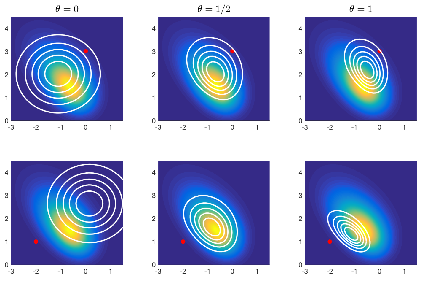
With an explicit expression for the transition density, we can investigate the stability of the iterates given by Algorithm 1. The most convenient way of doing this is by demonstrating geometric ergodicity of the chain induced by the transition kernel (6). Recall that a Markov chain with -fold transition kernel is said to be geometrically ergodic toward an invariant density if there exist constants and such that
Similarly, a diffusion process with transition kernel density is said to be exponentially ergodic towards an invariant density if there exist constants such that
It was shown in Hansen 2003 that the overdamped Langevin diffusion (1) is exponentially ergodic provided the following assumption on holds:
Assumption 2
Intuitively, 2 imposes super-Gaussian tails of the target distribution. Under Assumptions 1 and 2, for any and , there exists a constant depending on , such that (Lemma 6)
| (7) |
2 is not new, having also appeared in Kopec 2014, and appears to be among the weakest assumptions one can make to effectively study these implicit schemes. Clearly, Eq. 7 is a significantly weaker condition than strong convexity:
Assumption 3
The function is -strongly convex, that is, there exists such that
In fact, it is straightforward to show that if Assumption 2 holds, then is necessarily common in the two inequalities. Furthermore, we remark that under Assumptions 1 and 3, the spectrum of every Hessian matrix is controlled to be within . Strong convexity is quite a natural assumption in Bayesian regression problems, as it can be guaranteed for the class of GLMs with Gaussian priors (DasGupta 2011).
Under Assumptions 1 and 2, we can now establish geometric ergodicity of the -method scheme under certain conditions on and (Theorem 1).
Theorem 1
While Theorem 1 establishes the geometric ergodicity of the chain towards some stationary distribution, in general, that distribution need not necessarily be . Nevertheless, under Assumptions 1 and 3, we have established that the -method discretization of the overdamped Langevin equation is stable for any step size, provided . For these choices of , this implies that ILA is less strict about step size tuning than ULA. As will be seen in §5, this will prove to have a profound effect on the performance of ILA relative to ULA on high-dimensional problems.
2.2 Asymptotic exactness for the normal distribution
Among all values for , we draw special attention to the choice . This resulting integrator, also known as the trapezoidal scheme, is known to be second-order accurate when applied to ODEs; that is, for a quadratic function , iterates of the trapezoidal scheme for solving yield points of the exact solution (Süli and Mayers 2003, §12.4). An important consequence of this is that the global error incurred in the trapezoidal scheme is as . Unfortunately, as a consequence of the Itô calculus, this property does not hold for numerical solutions of stochastic differential equations. The construction of second-order schemes which are exact for quadratic in finite time and exhibit global error generally require careful treatment of the stochastic term—see for example Anderson and Mattingly 2011, or the Ozaki local linearization scheme (Biscay et al. 1996). However, when , the notion of second-order accuracy itself carries over to ILA in a rather remarkable way.
The case where is a quadratic form corresponds to sampling from a (multivariate) normal distribution , where
| (8) |
It is easy to see that, in this particular setting, Eq. 3 becomes explicitly solvable. Indeed, letting , we see that , and so
| (9) |
Observe that if is chosen to be a fixed value, all of the iterates are normally distributed. As a consequence of Lévy continuity, the stationary distribution of the ILA, if it exists, must also be normally distributed. In particular, due to (9), it must have mean and covariance satisfying
Since , it must be the case that . Solving for , the stationary distribution of the ILA is found to be
Here we encounter the remarkable fact that when is quadratic and , regardless of the step size chosen, ILA is asymptotically unbiased! To our knowledge, this was first observed in Wibisono 2018, however, as a consequence of our analysis, we can now deduce that is the only choice of that yields this property. While asymptotic exactness is unlikely to hold for other sampling problems, it suggests that cases involving approximately quadratic should see near optimal performance when .
3 Inexact Implicit Langevin Algorithm (i-ILA)
It is clear that the utility of ILA is dependent on the solvability of Eq. 3. Fortunately, this is made feasible by a useful reinterpretation of solutions to (3) as those of a corresponding optimization problem. Indeed, the inverse operator is quite commonly considered in convex optimization, as it is equivalent to the proximal operator defined by
This equivalence follows from that of an optimization problem and the root-finding problem for its critical values (Parikh and Boyd 2014, Eqn. (3.4)). Therefore, (3) can be formulated as the following optimization problem (after rescaling by ):
| (10a) | ||||
| where | ||||
| (10b) | ||||
This reinterpretation of (3) was also noted in Wibisono 2018, although only the case was considered. Iterations of the form (10) are often referred to as proximal-point methods in the optimization literature (Combettes and Pesquet 2011, Parikh and Boyd 2014). We remark that proximal operators were used in Pereyra 2016 in the construction of a proximal unadjusted Langevin algorithm (P-ULA). In fact, iterates of their P-ULA algorithm would correspond with (10) when and if the Gaussian term were to be moved outside the proximal operator. As one might expect, this discrepancy has a significant impact on the covariance of each proposal as ; it will be shown in Theorem 5 that the asymptotic covariance of these proposals is generally anisotropic.
The implementation of Algorithm 1 now hinges entirely on our ability to solve the subproblem Eq. 10. For the unadjusted Langevin algorithm where , this can be done trivially through a closed form solution. However, for , we generally have to resort to an iterative optimization scheme to solve Eq. 10. Thus far, we have assumed that the optimization problem in Eq. 10 can be solved exactly. However, more often than not this is infeasible, and one must instead consider the effects of approximate solutions of Eq. 10 in the overall convergence of the chain. This results in a sampling variant, which is henceforth referred to as i-ILA (for inexact ILA).
The most natural way of doing this is by measuring the error in the corresponding root-finding problem (3) via the norm of the gradient of the subproblem Eq. 10b, . This is ideal because not only can it be readily computed in practice, but also the termination criterion of many iterative optimization algorithms is based on this norm falling below a given tolerance; for example, see Nocedal and Wright 2006. Furthermore, efficient algorithms for directly minimizing , as a surrogate function for optimization of , have been recently proposed, which enjoy linear, that is, geometric, convergence rates, even in the absence of smoothness or convexity of (Roosta et al. 2018). In addition, for sampling in distributed computational environments, such as when large-scale data cannot be stored on a single machine, distributed variants of these surrogate optimization algorithms have also been recently considered (Crane and Roosta 2019). These algorithms are particularly suitable as part of i-ILA since they are guaranteed to rapidly and monotonically decrease ; recall that need not be monotonically decreasing in optimization algorithms that optimize directly.
With this in mind, we consider an inexact modification of Algorithm 1, shown in Algorithm 2, for approximate sampling from .
Find satisfying , where is defined in (10b) end for
3.1 Theoretical analysis of Algorithm 2
The increased stability offered by Algorithm 1 has been established in Theorem 1. However, while Theorem 1 guarantees rapid convergence towards some stationary distribution, closeness of the -method iterates to the target distribution and the effect of increasing on its bias as a sampling method, has yet to be established. Furthermore, Algorithm 1 and its guarantees given by Theorem 1 require exact solutions of the root-finding problem Eq. 3, whereas Algorithm 2 allows for such problems to be solved only inexactly. To address both of these problems, we devote this section to the development of theoretical guarantees of Algorithm 2, inspired by the techniques of Dalalyan 2017b. These guarantees come in the form of rate of convergence estimates under the 2-Wasserstein metric, defined between two probability measures and by
where the infimum is taken over all couplings of and , and is attained by some optimal coupling (Villani 2008, Thm. 4.1). The 2-Wasserstein metric can be readily linked to other quantities of interest. For example, from the Kantorovich-Rubinstein formula (Villani 2008, Eqn. (5.11)), for any -Lipschitz function , we have that
Our guarantees will require the same assumptions on seen in Dalalyan 2017b, that are Assumptions 1 and 3. Under these assumptions, the condition number of in Eq. 10b can be written as
| (11) |
Recall that the condition number Eq. 11 encodes and summarizes the curvature (the degree of relative flatness and steepness), of the graph of . In optimization, it is well-known that a large condition number typically amounts to a more difficult problem to solve, and hence algorithms that can take such contorted curvature into account (Newton-type methods, for example), are more appropriate (Roosta-Khorasani and Mahoney 2018, Xu et al. 2017). It is only natural to anticipate that challenges corresponding to problem ill-conditioning similarly carry over to sampling procedures as well. Indeed, large ratios of , which imply increasingly anisotropic level-sets for , can hint at more difficult sampling problems. For example, this difficulty directly manifest itself in ill-conditioning of , which in turn results in more challenging sub-problems. Furthermore, in such situations, taking a larger step size can only exacerbate the ill-condition of . As a result, similar to the role played by second-order methods in optimization, one can naturally expect to see implicit methods to be more appropriate for ill-conditioned sampling problems.
Under Assumptions 1 and 3, the discrepancy between the inexact variant of the -method given in Algorithm 2 and the target density under the 2-Wasserstein metric is described in Theorem 2.
Theorem 2
Remark 3
As , for the transition point we have . Moreover, at and , (15) coincides with Dalalyan and Karagulyan 2019, up to a different constant in the bias term. To see this, observe that implies , , when , and , when . This gives
Theorem 2 may thus be seen as a generalization of Dalalyan and Karagulyan 2019 to arbitrary and error .
Remark 4
In the noteworthy case of , Theorem 2 implies
As Theorem 1 did for Algorithm 1, Theorem 2 shows that for , Algorithm 2 is stable for all . Theorem 2 does suggest that smaller values of will achieve faster convergence rates and smaller biases for small step sizes, although this does not appear to be the case in practice (for example, refer to §5). Observe that, for and fixed , the bias term is in the order of . This implies that increasing the condition number when is bounded below (for example the spherical Gaussian prior in Bayesian regression) results in smaller bias and faster convergence. This is in sharp contrast to ULA whose performance significantly degrades with increasing condition number in such settings.
Also, we would like to reiterate that, in stark contrast to what is observed in Roberts and Rosenthal 2001 for Metropolis-Hastings algorithms, the rate of convergence in Theorem 2 for Algorithm 2 is not dependent on the dimension in any form other than through the appearances of and . The dimension appears in the bias term simply due to the natural expansion of the Euclidean distance with dimension. In particular, following Durmus and Moulines 2019, as the dependence on dimension is at most polynomial, this lends credence to the claim that implicit Langevin methods are well-equipped to handle high-dimensional sampling problems.
4 Asymptotics for large step size
While Theorem 2 provides an essential description of the behavior of Algorithm 2, the bounds presented there are tightest for smaller step sizes on the order of , and are less effective when is larger. Unfortunately, the most useful applications of ILA will occur when is large, and so the small step size () regime will not be all that relevant. Enabled by the increased stability of ILA, we present a novel analysis of Algorithm 1 by establishing a central limit-type theorem regarding asymptotic behavior of the iterates in the regime.
Before we begin with a formal analysis, we are able to obtain insight by considering the behavior of the subproblem Eq. 10 as . For , we have
where does not depend on , and so does not contribute to solving (10). As a result, the iterates of the method in the regime will satisfy the relations , where we let
| (16) |
Letting denote the unique mode of , iterating (16) gives
where . Under Assumption 3, we obtain
Therefore, the behavior of the -method for large is determined according to the three regimes depicted in Table 1.
| (unbounded in probability) | ||
| iterates oscillate about the mode | ||
| (collapse to the mode) |
The case is clearly undesirable from a practical standpoint. Moreover, the collapse towards the mode seen when is close to one suggests enormous potential bias for large step sizes. On the other hand, the case provides no damping effect whatsoever (a fact also supported by Theorem 2), making it susceptible to rare large proposals. Based on this preliminary analysis, for some small , a choice of appears to provide the safest, and potentially the most accurate of our -method samplers. This aligns with the rule-of-thumb used for -method discretization of ODEs (Ascher 2008, p. 85). To formally extend these characterizations to the implicit -method scheme Eq. 3, in Theorem 5, a central limit theorem as is obtained for a single step of the scheme about the deterministic map .
Theorem 5
Given any , consider iterations given by Eq. 10, where . Conditioned on , we have
Theorem 5 implies that as , the implicit -method scheme behaves similarly to a Markov chain with transitions
whose dynamics mimic those of the map , but with an additional normally-distributed noise term at each step. Furthermore, the variance of this noise term increases as the implicit component of the scheme diminishes (taking ). Despite the unusual regime, we have found that, for typical step sizes, Theorem 5 provides a surprisingly accurate description of the transition dynamics of ILA when , and is ideal for developing heuristics.
4.1 A heuristic choice for step size
A consequence of the proof of Theorem 5 is that the covariance of the proposal density from the transition kernel behaves asymptotically as
Conversely, applying the inverse function theorem to (4) reveals a linear approximation about , and hence
These two expressions coincide when , where denotes the mode. At this point, one might expect a ‘good’ transition kernel to resemble the Laplace approximation of the distribution about , which has covariance . This suggests a heuristic for choosing a good step size in practice, by taking as a solution to the one-dimensional optimization problem
| (17) |
where the norm can be any matrix norm of choice. Solutions to (17) can be obtained using off-the-shelf methods in univariate optimization, such as golden section search (Cottle and Thapa 2017, §9.5). We will show in the next section that, for several examples, the step size obtained from Eq. 17 with Frobenius norm tends to be an effective choice in practice, especially for , where it reveals itself to be near optimal in all of our experiments. For this choice of norm, Eq. 17 can be replaced by the equivalent problem
| (18) |
where are the eigenvalues of . One drawback is that solving (17) or (18) require either inversion of ), or knowledge of its spectrum, respectively, both of which may be prohibitively expensive in high dimensions. In many problems, however, it is reasonable to assume a certain distribution of its spectrum; for example, that the eigenvalues of decay exponentially:
| (19) |
where and take the place of the smallest and largest eigenvalues of , respectively. Simplifying assumptions such as these can be justified in problems where Hessian of is approximately low rank, in the sense that it has a small stable rank (Roosta-Khorasani and Ascher 2015), and hence its spectrum decays fast. Under these assumptions, solving Eq. 18 becomes more tractable; we shall make use of this for Fig. 3 in §5.
5 Numerical experiments
In this section, we evaluate the empirical performance of Algorithms 1 and 2 in high-dimensions as measured by a few discrepancy measures. Recall that the total variation distance between any two absolutely continuous distributions with densities and over respectively is given by
Since the total variation metric is too difficult to directly estimate in higher dimensions, we follow the standard approach in the literature (see for example Durmus and Moulines 2019 and Maire et al. 2018) and consider instead the mean marginal total variation (MMTV),
which we estimate as follows. First, kernel smoothing is applied to samples for each marginal from an extended MCMC run, as well as samples obtained from a single run of each method. The total variation between these estimated univariate densities is then computed with high accuracy via Gauss-Kronrod quadrature (Kahaner et al. 1989).
As a weakness of MMTV is its inability to adequately compare the covariances within coordinates between the two sample sets, we also compare with a second discrepancy measure; maximum mean discrepancy (MMD) (Gretton et al. 2012, Muandet et al. 2017). Letting denote a reproducing kernel Hilbert space over with reproducing kernel , MMD is defined as the integral probability metric
where are independent random variables with distribution , and are independent random variables with distribution . These expectations can be estimated using samples from and . In our experiments, we use the Gaussian kernel:
where the kernel bandwidth parameter is chosen so that is the median of , where denotes the -th sample taken from .
5.1 High-dimensional Gaussian distributions
To highlight the effects of problem ill-conditioning, we once again consider sampling from a multivariate Gaussian distribution, as in (8), with explicitly computable iterates given by (9). It is easy to see that satisfies Assumptions 1 and 3. To show efficacy in higher dimensions, we will consider . Furthermore, to test the effects of ill-conditioning, we focus on three choices of with condition numbers . Each is generated using the method of Bendel and Mickey 1978 to uniformly sample a correlation matrix with eigenvalues given by (19) for and . For simplicity, we take . MMTV and MMD discrepancies were computed between and samples of points generated by Algorithm 1 with and a variety of step sizes (encompassing and the step size heuristics in §4). Common random numbers were used, and no burn-in period was applied. The results are shown in Figure 2.
| Mean Marginal Total Variation | Maximum Mean Discrepancy |
| : | |
|---|---|
| : | |
| : |
Due to the rapid explosion in magnitude of samples generated by ULA when , we only display discrepancies for ULA for . This critical value of is highlighted as a black solid vertical line.
In light of the large step size asymptotics, the existence of an “optimal” step size for as evidenced in these plots is perhaps not too surprising. However, it is surprising to see that, especially for large , this optimum is much greater than the maximum allowed step size of for ULA. Most notable here is the greatly improved performance of the implicit method () at this optimum over ULA for any allowable step size. Moreover, in all cases, the optimal performance of ILA for exceeds that of the purely implicit method (). These two facts are not suggested by Theorem 2, implying that the large step size asymptotics should indeed play a significant role in the analysis of implicit methods moving forward.
In all cases, the step size heuristic for performs poorly, suggesting the fully implicit case operates by a different mechanism that is currently unknown to us. For , , which is clearly the optimal step size, as it yields exact samples (). In fact, , is the only choice of and which results in exact samples in this scenario. According to both estimated MMTV and MMD, the step size heuristic is an almost optimal choice of for all considered, even in high dimensions.
5.2 Logistic regression
We now consider sampling problems involving the Bayesian posterior densities of generalized linear models (GLM), which have log-concave likelihood functions, with Gaussian priors. For simplicity, and without loss of generality, we consider radially symmetric Gaussians. For a GLM with this choice of prior, posterior densities are proportional to , with
where are the response and covariate pairs, , and the domain of depends on the GLM. The cumulant generating function, , determines the type of GLM. For example, in the case of logistic regression, ; see McCullagh and Nelder 1989 for further details and applications. It is easy to see that
where is a matrix whose -th row is , is a diagonal matrix whose -th diagonal element is , and is the precision parameter of the prior. As a result, for Assumption 3, we have
| (20) |
For our example, we consider Bayesian logistic regression in this setting, yielding
| (21) |
and . We use the musk (version 1) data set from the UCI repository (Dua and Graff 2019), with the prior precision parameter . These choices yield a target distribution which is relatively ill-conditioned, whose Hessian about its mode possesses a condition number of . We estimate the values and according to their lower and upper bounds in (20). For the target density given according to (21), MMTV and MMD discrepancies were computed between samples of points generated using Algorithm 2 (with , and a variety of step sizes encompassing and the step size heuristics in §4 under the assumption that eigenvalues are distributed according to Equation 19) and a gold standard run comprised of 50,000 samples obtained from hand-tuned SMMALA (Girolami and Calderhead 2011). Due to the large difference in computation time between ULA and ILA, for the sake of comparison, we also computed MMTV and MMD discrepancies for the ULA algorithm using the same step sizes, now with a thinning factor of 50. This factor was chosen so that the computation time of ULA became roughly equivalent to the other ILA methods. Once again, common random numbers were used, and no burn-in period was applied. The results are shown in Figure 3, and follow a similar pattern to those found in the previous example. The step size heuristic for performs admirably in this case, yielding samples with smaller discrepancies to the gold standard run than ULA for any reasonable step size, even when thinned to account for the difference in computation time.
6 Conclusions
In the context of sampling from an unnormalized probability distribution, we considered a general class of unadjusted sampling algorithms that are based on implicit discretization of the Langevin dynamics. Unlike the traditional Metropolis-adjusted sampling algorithms, these unadjusted methods relax the requirement of consistency that the sample empirical distribution should asymptotically be the same as the target distribution, and hence avoid incurring serious penalty to the mixing rate of the chain. As a result, these variants generate rapidly converging Markov chains whose stationary distributions are only approximations of the target distribution with a bias that is of adjustable size. When one seeks a fixed (finite) number of samples, which is almost always the case in practice, this latter unadjusted view point can offer greatly many advantages.
In this context, we focused on the class of discretization schemes generated using -method in the context of smooth and strongly log-concave densities, explicitly deriving the transition kernel of the chain and establishing the corresponding sub-problems that are formulated as optimization problems. For smooth densities, the resulting implicit Langevin algorithms (ILA) have been shown to be geometrically ergodic for , irrespective of the step size. We also considered inexact variants (i-ILA) where the optimization sub-problems are solved only approximately. For this, we established non-asymptotic convergence of the sample empirical distribution to the target as measured by 2-Wasserstein metric, finding again that for , the resulting scheme is unconditionally stable for all step sizes. Furthermore, the growth rate in the bias term, that is shown to depend on problem’s condition number, is greatly diminished for . Together with our numerical experiments, this suggests that the implicit methods are a more appropriate choice for ill-conditioned problems than explicit schemes. Furthermore, the case appears to perform best in practice, especially when paired with our default heuristic choice of step size. The underlying reason for this is likely related to its asymptotic exactness for the normal distribution. It was suggested in Wibisono 2018 that the asymptotic bias of the case could be second-order accurate, which would imply the increased performance we have observed. Unfortunately, proving this claim remains an open problem.
Although enticing, extensions of these results to non-convex cases may prove challenging due to the potential lack of unique solutions for the implicit scheme, and the relative difficulty of non-convex optimization in general. Nevertheless, one could find success in considering that is only strongly convex outside of a compact region, as in Cheng et al. 2018a. Furthermore, although it has not been treated explicitly, we believe that implicit methods should prove effective in big data problems, that is with and , where it might be computationally prohibitive to evaluate or its gradient exactly. In this regard, one can use optimization algorithms that can employ inexact oracle information; see Roosta-Khorasani and Mahoney 2018 for example. The efficacy of this approach would prove interesting for future research.
7 Acknowledgements
All authors have been supported by the Australian Centre of Excellence for Mathematical and Statistical Frontiers (ACEMS) under grant number CE140100049. Liam Hodgkinson acknowledges the support of an Australian Research Training Program (RTP) Scholarship. Fred Roosta was partially supported by the Australian Research Council through a Discovery Early Career Researcher Award (DE180100923). Part of this work was done while Fred Roosta was visiting the Simons Institute for the Theory of Computing.
Appendix A Proofs
A.1 Proof of Theorem 1 (Geometric Ergodicity)
To establish geometric ergodicity, we prove the stronger Proposition 8 below. First, we connect Assumptions 1 and 2 to the lower bound (7).
Proof By 1, observe that for any , we have
Hence, we have
The result is implied by the definition of limit infimum.
To state the result, we recall the definition of -uniform ergodicity, as seen
in Meyn and Tweedie 2012.
Definition 7 (-uniform ergodicity)
A -ergodic Markov chain with Markov transition operator on is -uniformly ergodic for a measurable function if
By Meyn and Tweedie 2012, any -uniformly ergodic Markov chain is also geometrically ergodic.
Proposition 8
Proof It is immediately apparent from the positivity of (6) due to (5) that the iterates of the -method scheme are aperiodic and irreducible with respect to Lebesgue measure. Furthermore, it follows from Meyn and Tweedie 2012 that all compact sets are small. Therefore, by Meyn and Tweedie 2012 and Meyn and Tweedie 2012, it suffices to show that
where is the Markov transition operator of the -method scheme. Indeed, by the definition of , for a given , there exists a such that
and so for any . Letting denote the first step of the -method scheme starting from , (4) implies
Thus, by letting , we obtain , where
By the reverse triangle inequality, for any , and hence, is -Lipschitz in . Consequently, we can apply the Gaussian concentration inequality (Boucheron et al. 2013, Theorem 5.5) to reveal
Since by Jensen’s inequality,
It follows that
where
Therefore, if we can show that as , then the result follows. Since , we may focus on the difference of the squares:
| (23) |
where the last inequality follows from (7). Provided that or , (23) will be negative for sufficiently large . Since also
for any and sufficiently large ,
which implies the difference as , as required.
A.2 Proof of Theorem 2 ( bounds)
Next, using techniques analogous to those of Dalalyan and Karagulyan 2019, we prove Theorem 2. For the sake of brevity, we let denote the minimum of any two quantities and . The following estimate is fundamental to the argument.
Lemma 9
Let be the solution to the (overdamped) Langevin equation
for such that is -Lipschitz continuous. Then for any , if ,
Proof Since is stationary, for any , by Dalalyan 2017a. Therefore, . Furthermore, following the same procedure as in Dalalyan and Karagulyan 2019
With Lemma 9 in hand, we may proceed with the proof of the main result.
Proof [Theorem 2] Letting denote a -dimensional standard Brownian motion independent of and , define the stochastic process by
Evidently, is a realization of (1) and so is a reversible Markov process with for every . Now, couple the inexact -method scheme satisfying
for an appropriate error term , to , by letting for each , and choosing such that . Observing that, for any ,
by construction, . For each , let , observing that and . Choosing some , for the sake of brevity, we denote , which now satisfies
Altogether, we have
where
An application of the fundamental theorem of calculus implies and , where
Altogether, where and
It can be verified using induction that the solution to this first-order non-homogeneous recurrence relation is given by
Now, observe that by denoting , for any ,
| (24) |
Since the eigenvalues of are bounded above by and below by , so too are the eigenvalues of for each . Therefore,
| (25) |
The transition between these regimes occurs at the point which is the solution to
over . Equivalently, it is the solution to
and therefore to the quadratic equation
It may be readily verified that as defined in (12) is the only positive solution. Furthermore, provided that or . Also, for any ,
| (26) |
which further implies for any . Now combining (24), (25), and (26), for , , and hence, altogether,
Since is reversible and stationary, , and by Lemma 9, . Therefore
Since
applying the closed-form expression for the geometric series,
and the result follows.
A.3 Proof of Theorem 5 (Central Limit Theorem)
Proof The proof makes use of Laplace’s method. From Eq. 6 and the change of variables theorem, the Markov kernel for the transition is given by
| (27) |
Letting where , it suffices to show that as , pointwise in . Denoting , since , the exponent of (27) becomes
Since and the determinant term converges to , the
result follows.
References
- Anderson and Mattingly (2011) David Anderson and Jonathan Mattingly. A weak trapezoidal method for a class of stochastic differential equations. Communications in mathematical sciences, 9:301–318, 03 2011.
- Ascher (2008) Uri M. Ascher. Numerical methods for evolutionary differential equations. SIAM, 2008.
- Ascher and Petzold (1998) Uri M. Ascher and Linda Petzold. Computer Methods for Ordinary Differential Equations and Differential-Algebraic Equations. Other Titles in Applied Mathematics. Society for Industrial and Applied Mathematics (SIAM, 3600 Market Street, Floor 6, Philadelphia, PA 19104), 1998. ISBN 9781611971392.
- Bendel and Mickey (1978) Robert B. Bendel and M. Ray Mickey. Population correlation matrices for sampling experiments. Communications in Statistics-Simulation and Computation, 7(2):163–182, 1978.
- Biscay et al. (1996) R. Biscay, J. C. Jimenez, J. J. Riera, and P. A. Valdes. Local linearization method for the numerical solution of stochastic differential equations. Annals of the Institute of Statistical Mathematics, 48(4):631–644, 1996.
- Bishop and Tipping (2003) Christopher M. Bishop and Michael E. Tipping. Bayesian regression and classification. Nato Science Series sub Series III Computer And Systems Sciences, 190:267–288, 2003.
- Boucheron et al. (2013) Stéphane Boucheron, Gábor Lugosi, and Pascal Massart. Concentration inequalities: A nonasymptotic theory of independence. Oxford university press, 2013.
- Casella et al. (2011) Bruno Casella, Gareth Roberts, and Osnat Stramer. Stability of partially implicit Langevin schemes and their MCMC variants. Methodology and Computing in Applied Probability, 13(4):835–854, December 2011.
- Chatfield et al. (2010) Chris Chatfield, Jim Zidek, and Jim Lindsey. An introduction to generalized linear models. Chapman and Hall/CRC, 2010.
- Cheng and Bartlett (2018) Xiang Cheng and Peter Bartlett. Convergence of Langevin MCMC in KL-divergence. In Proceedings of Algorithmic Learning Theory, volume 83, pages 186–211, 2018.
- Cheng et al. (2018a) Xiang Cheng, Niladri S. Chatterji, Yasin Abbasi-Yadkori, Peter L. Bartlett, and Michael I. Jordan. Sharp Convergence Rates for Langevin Dynamics in the Nonconvex Setting. arXiv preprint arXiv:1805.01648, 2018a.
- Cheng et al. (2018b) Xiang Cheng, Niladri S. Chatterji, Peter L. Bartlett, and Michael I. Jordan. Underdamped Langevin MCMC: A non-asymptotic analysis. In Sébastien Bubeck, Vianney Perchet, and Philippe Rigollet, editors, Proceedings of the 31st Conference On Learning Theory, volume 75 of Proceedings of Machine Learning Research, pages 300–323. PMLR, 06–09 Jul 2018b.
- Combettes and Pesquet (2011) Patrick L. Combettes and Jean-Christophe Pesquet. Proximal splitting methods in signal processing. In Fixed-point algorithms for inverse problems in science and engineering, pages 185–212. Springer, 2011.
- Cottle and Thapa (2017) Richard W. Cottle and Mukund N. Thapa. Linear and Nonlinear Optimization. International Series in Operations Research & Management Science. Springer New York, 2017. ISBN 9781493970537.
- Crane and Roosta (2019) Rixon Crane and Fred Roosta. DINGO: Distributed Newton-type method for gradient-norm optimization. In Advances in Neural Information Processing Systems, pages 9494–9504, 2019.
- Dalalyan (2017a) Arnak S. Dalalyan. Further and stronger analogy between sampling and optimization: Langevin Monte Carlo and gradient descent. arXiv preprint arXiv:1704.04752, 2017a.
- Dalalyan (2017b) Arnak S. Dalalyan. Theoretical guarantees for approximate sampling from smooth and log-concave densities. Journal of the Royal Statistical Society: Series B (Statistical Methodology), 79(3):651–676, 2017b.
- Dalalyan and Karagulyan (2019) Arnak S Dalalyan and Avetik Karagulyan. User-friendly guarantees for the Langevin Monte Carlo with inaccurate gradient. Stochastic Processes and their Applications, 129(12):5278–5311, 2019.
- DasGupta (2011) Anirban DasGupta. Probability for Statistics and Machine Learning: Fundamentals and Advanced Topics. Springer Texts in Statistics. Springer New York, 2011. ISBN 9781441996336.
- Dua and Graff (2019) Dheeru Dua and Casey Graff. UCI machine learning repository, 2019. URL http://archive.ics.uci.edu/ml.
- Durmus and Moulines (2017) Alain Durmus and Eric Moulines. Nonasymptotic convergence analysis for the unadjusted Langevin algorithm. The Annals of Applied Probability, 27(3):1551–1587, 2017.
- Durmus and Moulines (2019) Alain Durmus and Eric Moulines. High-dimensional Bayesian inference via the unadjusted Langevin algorithm. Bernoulli, 25(4A):2854–2882, 2019.
- Girolami and Calderhead (2011) Mark Girolami and Ben Calderhead. Riemann manifold Langevin and Hamiltonian Monte Carlo methods. Journal of the Royal Statistical Society: Series B (Statistical Methodology), 73(2):123–214, 2011.
- Golub and Van Loan (2012) Gene H. Golub and Charles F. Van Loan. Matrix Computations, volume 3. JHU Press, 4 edition, 2012.
- Gretton et al. (2012) Arthur Gretton, Karsten M. Borgwardt, Malte J. Rasch, Bernhard Schölkopf, and Alexander Smola. A kernel two-sample test. Journal of Machine Learning Research, 13(Mar):723–773, 2012.
- Hansen (2003) Niels Richard Hansen. Geometric ergodicity of discrete-time approximations to multivariate diffusions. Bernoulli, 9(4):725–743, 2003.
- Hastings (1970) Wilfred K. Hastings. Monte Carlo sampling methods using Markov chains and their applications. Biometrika, 57(1):97–109, 1970. ISSN 00063444.
- Ikeda and Watanabe (2014) Nobuyuki Ikeda and Shinzo Watanabe. Stochastic differential equations and diffusion processes, volume 24. Elsevier, 2014.
- Kahaner et al. (1989) David Kahaner, Cleve B. Moler, Stephen Nash, and George E. Forsythe. Numerical Methods and Software. Prentice-Hall series in computational mathematics. Prentice Hall, 1989.
- Kloeden and Platen (2013) Peter E. Kloeden and Eckhard Platen. Numerical solution of stochastic differential equations, volume 23. Springer Science & Business Media, 2013.
- Kolmogorov (1937) Andrei N. Kolmogorov. Zur umkehrbarkeit der statistischen naturgesetze. Mathematische Annalen, 113(1):766–772, 1937.
- Kopec (2014) Marie Kopec. Weak backward error analysis for overdamped Langevin processes. IMA Journal of Numerical Analysis, 35(2):583–614, 2014.
- Korattikara et al. (2014) Anoop Korattikara, Yutian Chen, and Max Welling. Austerity in MCMC land: Cutting the Metropolis-Hastings budget. In International Conference on Machine Learning, pages 181–189, 2014.
- Lambert (1991) John Denholm Lambert. Numerical methods for ordinary differential systems: the initial value problem. John Wiley & Sons, Inc., 1991.
- Maire et al. (2018) Florian Maire, Nial Friel, and Pierre Alquier. Informed sub-sampling MCMC: approximate Bayesian inference for large datasets. Statistics and Computing, pages 1–34, Jun 2018.
- Mattingly et al. (2002) Jonathan C. Mattingly, Andrew M. Stuart, and Desmond J. Higham. Ergodicity for SDEs and approximations: locally Lipschitz vector fields and degenerate noise. Stochastic processes and their applications, 101(2):185–232, 2002.
- McCullagh and Nelder (1989) Peter McCullagh and John A. Nelder. Generalized linear models, volume 37. CRC press, 1989.
- Meyn and Tweedie (2012) Sean P. Meyn and Richard L. Tweedie. Markov chains and stochastic stability. Springer Science & Business Media, 2012.
- Muandet et al. (2017) Krikamol Muandet, Kenji Fukumizu, Bharath Sriperumbudur, and Bernhard Schölkopf. Kernel mean embedding of distributions: A review and beyond. Foundations and Trends® in Machine Learning, 10(1-2):1–141, 2017.
- Nocedal and Wright (2006) Jorge Nocedal and Stephen Wright. Numerical Optimization. Springer Science & Business Media, 2006.
- Parikh and Boyd (2014) Neal Parikh and Stephen Boyd. Proximal Algorithms. Foundations and Trends® in Optimization, 1(3):127–239, 2014.
- Pereyra (2016) Marcelo Pereyra. Proximal Markov Chain Monte Carlo algorithms. Statistics and Computing, 26(4):745–760, Jul 2016. ISSN 1573-1375.
- Robert and Casella (1999) Christian P. Robert and George Casella. Monte Carlo Statistical Methods. Springer texts in statistics. Springer, 1999. ISBN 9780387987071.
- Roberts and Rosenthal (2001) Gareth O. Roberts and Jeffrey S. Rosenthal. Optimal scaling for various Metropolis-Hastings algorithms. Statistical science, 16(4):351–367, 2001.
- Roberts and Tweedie (1996) Gareth O. Roberts and Richard L. Tweedie. Exponential convergence of Langevin distributions and their discrete approximations. Bernoulli, 2(4):341–363, 12 1996.
- Rockafellar (1976) R Tyrrell Rockafellar. Monotone operators and the proximal point algorithm. SIAM journal on control and optimization, 14(5):877–898, 1976.
- Roosta et al. (2018) Fred Roosta, Yang Liu, Peng Xu, and Michael W. Mahoney. Newton-MR: Newton’s Method Without Smoothness or Convexity. arXiv preprint arXiv:1810.00303, 2018.
- Roosta-Khorasani and Ascher (2015) Farbod Roosta-Khorasani and Uri M. Ascher. Improved bounds on sample size for implicit matrix trace estimators. Foundations of Computational Mathematics, 15(5):1187–1212, 2015.
- Roosta-Khorasani and Mahoney (2018) Farbod Roosta-Khorasani and Michael W. Mahoney. Sub-sampled Newton methods. Mathematical Programming, Nov 2018.
- Shao (2008) Jun Shao. Mathematical Statistics. Springer Texts in Statistics. Springer New York, 2008. ISBN 9780387217185.
- Süli and Mayers (2003) Endre Süli and David F. Mayers. An introduction to numerical analysis. Cambridge University Press, 2003.
- Villani (2008) Cédric Villani. Optimal Transport: Old and New, volume 338. Springer Science & Business Media, 2008.
- Wibisono (2018) Andre Wibisono. Sampling as optimization in the space of measures: The Langevin dynamics as a composite optimization problem. In Sébastien Bubeck, Vianney Perchet, and Philippe Rigollet, editors, Conference On Learning Theory, COLT 2018, Stockholm, Sweden, 6-9 July 2018, volume 75 of Proceedings of Machine Learning Research, pages 2093–3027. PMLR, 2018.
- Xu et al. (2017) Peng Xu, Fred Roosta, and Michael W Mahoney. Newton-type methods for non-convex optimization under inexact Hessian information. Mathematical Programming, pages 1–36, 2017.