跳到论文正文
W Papers独立论文阅读器 arXiv:1903.12202 论文正文 计算阅读时间 · 0%
引用这篇论文根据当前论文元数据生成,正式投稿前建议核对。


License: arXiv.org perpetual non-exclusive license
arXiv:1903.12202v1 [physics.optics] 28 Mar 2019

When topological derivatives met regularized Gauss-Newton iterations in holographic 3D imaging

A. Carpio Note: Universidad Complutense de Madrid, Madrid 28040, Spain, and Courant Institute, New York University, NY 10012, USA    T.G. Dimiduk Note: Tesla, Palo Alto, CA 94304, USA    F. Le Louër Note: Université de Technologie de Compiègne, 60203 Compiègne, France    M.L. Rapún Note: Universidad Politécnica de Madrid, Madrid 28040, Spain

Abstract. We propose an automatic algorithm for 3D inverse electromagnetic scattering based on the combination of topological derivatives and regularized Gauss-Newton iterations. The algorithm is adapted to decoding digital holograms. A hologram is a two-dimensional light interference pattern that encodes information about three-dimensional shapes and their optical properties. The formation of the hologram is modeled using Maxwell theory for light scattering by particles. We then seek shapes optimizing error functionals which measure the deviation from the recorded holograms. Their topological derivatives provide initial guesses of the objects. Next, we correct these predictions by regularized Gauss-Newton techniques. In contrast to standard Gauss-Newton methods, in our implementation the number of objects can be automatically updated during the iterative procedure by new topological derivative computations. We show that the combined use of topological derivative based optimization and iteratively regularized Gauss-Newton methods produces fast and accurate descriptions of the geometry of objects formed by multiple components with nanoscale resolution, even for a small number of detectors and non convex components aligned in the incidence direction. The method could be applied in general imaging set-ups involving other waves (microwave imaging, elastography…) provided closed-form expressions for the topological and Fréchet derivatives are determined.

1 Introduction

Digital in-line holography is a promising tool for high speed three dimensional (3D) imaging of live cells and soft matter [21, 44]. It can achieve high temporal (microseconds) and spatial (nanometers) resolution while avoiding the usage of toxic stains and fluorescent markers. Holograms are two-dimensional (2D) light interference patterns that contain information about the 3D positions and optical properties of an object or set of objects [56]. Figure 1 illustrates the formation of an in-line hologram from the interference of the light field scattered from a sample and the undiffracted beam [34]. In tracking experiments, one expects to infer the position of objects as a function of time analyzing a time-series of holograms. Instead, in characterization experiments, one aims to extract the size, shape and refractive index of the particles under study. Traditional optical reconstructions shine light back through the hologram to produce a 3D image, though this process may introduce a number of artifacts for sizes comparable to the employed light wavelength [54]. In contrast, digital holography aims to achieve numerical reconstructions, facing the inherent difficulty of computationally recovering 3D geometries from the 2D holograms they generate. From the mathematical point of view, finding objects and their optical properties from holograms is an ill-posed inverse scattering problem.

(a)                  (b)
Refer to caption     Refer to caption

Figure 1: (a) A typical optical set-up to record in-line holograms. A collimated laser beam illuminates a sample. The resulting hologram is recorded on a CMOS camera. (b) Schematic representation of an in-line holography set-up used in the algorithms and simulations presented in this paper. The incident reference wave ℰinc{\mathbfcal E}_{\rm inc} interacts with the sample Ω\Omega generating a scattered wave ℰsc{\mathbfcal E}_{\rm sc}. The interference pattern created by both of them forms the hologram ℐmeas=|ℰinc+ℰsc|2{\mathbfcal I}_{\rm meas}=|{\mathbfcal E}_{\rm inc}+{\mathbfcal E}_{\rm sc}|^{2}. We have superimposed on the CMOS screen the hologram created by a sphere placed at a distance zs=5​μz_{s}=5\,\mum (1​μ1\mum=10−610^{-6} m) from that screen, when a 660660 nm (11 nm=10−910^{-9} m) laser is emitted.

Recent work has relied on scattering theory to analyze holograms. As demonstrated in [52, 53], in-line holograms can be predicted combining Lorenz-Mie scattering theory with a model for the propagation and interference of the light fields in the microscope. Later, spherical colloidal particles were successfully tracked and characterized by fitting scattering models based on the Lorenz-Mie theory to holograms [34]. More general scattering approximations allow to treat non-spherical particles like rods as well as clusters of spherical particles [21, 59] fitting to the data a forward model, that is, a model that can evaluate a hologram based on a theory of scattering and propagation inside the microscope, using solvers such as discrete dipole approximations (DDA), see for instance [58, 59]. These methods proceed by ‘least squares fitting’: a few parameters representing radius, orientation, position, refractive index and so on are adjusted iteratively by a Levenberg-Marquardt algorithm to minimize the error when comparing the synthetic holograms generated by the approximate objects as predicted by the selected forward model and the true measured hologram. Alternative bayesian and machine learning approaches are discussed in [15, 57]. Successful reconstructions typically require significant a priori knowledge about the objects being imaged, such as their approximate positions in the field of view and a simple parametrization (sphere, cylinder…), for example.

To track and characterize objects without a priori knowledge (other than the optical properties of the ambient medium and the incident light) we may formulate more comprehensive optimization problems. The idea is to optimize the error functionals with respect to arbitrary shapes and arbitrary functions representing the imaged objects and their optical properties. When illuminating simple object configurations with time harmonic and polarized light, the problem somewhat simplifies, since we can use scalar Helmholtz approximations to simulate the polarized component of light [5, 6]. Within this simplified framework, Ref. [6] succeeds in producing first guesses of objects and of their optical properties from the holograms they generate by combining topological derivative and gradient based optimization procedures, provided the size of the objects is of the same order or smaller than the employed light wavelength. Helmholtz equations for the forward problems are solved in [6] by coupled boundary element (BEM)/finite element (FEM) methods [48, 51], whereas shapes are constructed by means of blobby molecule coverings and signed distance functions as in [5], without imposing any specific parametrization.

Instead of relying on particular scattering theories, here we implement topological derivative based optimization using the 3D vector Maxwell equations, which requires new closed-form formulas adapted to the holographic setting. We obtain them extending ideas developed in [6] to deal with holograms I=|𝐄|2I=|{\mathbf{E}}|^{2} under scalar approximations for polarized light to derivations for error functionals using complex measured data 𝐄\bf E and vector Maxwell constraints [47, 8, 36, 37]. As it happens in other imaging problems (acoustics, elastography…), topological derivatives allow us to generate first guesses of holographied objects and to correct the number of boundaries by creating, merging or destroying components. However, topological derivative based iterations may get stuck without providing a precise description of the shapes unless data distributed over a wide enough angle for a wide enough range of frequencies or incoming incident directions are available [1, 7, 8, 26]. We find that this is the case in holography. Due to the way microscopes are built, only one incident direction and one frequency are usually available and data are measured on a limited screen behind the object [5, 34, 59]. Moreover, our tests show that the results do not really improve switching to optimization procedures that deform the approximate object contours along vector fields, such as shape derivative based deformations or level set techniques [9, 17, 28, 46]. In this paper, we overcome this difficulty by combining topological derivative based optimization with iteratively regularized Gauss-Newton methods, see the videos in the supplemental material. For the true objects we will only require 𝒞2{\cal C}^{2} regularity. However, those objects will be approximated by star-shaped components during the iterative procedure. Star-shaped objects are defined by rays emerging from one fixed position 𝐜\mathbf{c}. Their boundary is located at distances of that point which vary with the angles. Therefore, they can be described using a spherical coordinate system, as it happens for ellipsoids and smoothed polyhedra, for instance. A general object formed by several star-shaped components is represented as Ω=∪ℓ=1ℒΩℓ,\Omega=\cup_{\ell=1}^{\cal L}\Omega_{\ell}, ∂Ωℓ=𝐜ℓ+𝐫ℓ​(𝕊2),\partial\Omega_{\ell}=\mathbf{c}_{\ell}+\mathbf{r}_{\ell}(\mathbb{S}^{2}), where 𝐫ℓ:𝕊2→ℝ3\mathbf{r}_{\ell}:\mathbb{S}^{2}\rightarrow\mathbb{R}^{3} is a combination of spherical harmonics. Our method identifies automatically the number of defects ℒ{\cal L} (i.e., we do not assume ℒ{\cal L} to be known), and provides the centers 𝐜ℓ\mathbf{c}_{\ell} and the radii functions 𝐫ℓ\mathbf{r}_{\ell} defining our approximation of the true configuration, which does not need to consist in star-shaped objects. Furthermore, the method could be extended to a broader class of parameterizations dropping the star-shaped constraint, see [27]. To simplify, we assume that the optical properties are known and constant inside each component.

The starting point of our algorithm are star-shaped parametrizations fitted to initial guesses of the holographied objects provided by topological derivative optimization of the error functional comparing the synthetic hologram generated by any object with the true hologram. Next, we linearize the synthetic hologram contribution in this quadratic error functional about the current parametrization to obtain a nonlinear least squares problem for the next star-shaped parametrization, which is regularized including a Tikhonov quadratic term. Gauss-Newton iterations are a very powerful tool for finding the best descent direction for minimizing nonlinear least squares problems [2, 31, 32, 27]. There is work on coupling topological gradients and Gauss-Newton iterations [19] to solve a 2D inverse problem in elasticity, applied to parameter reconstruction instead of shape reconstruction. That study does not consider the iteratively regularized Gauss-Newton method whose regularizing Tikhonov parameter is exponentially decreasing to ensure the convergence of the algorithm [31, 32] when the stoppping rule is given by Morozov’s discrepancy principle, as we do here. Moreover, the classical application of the iteratively regularized Gauss-Newton method requires an initial guess formed by the true number of components, while our hybrid method does not: it automatically updates this number by topological derivative computations. This is the key starting point for constructing automatic/smart inverse algorithms. The hybrid inverse algorithm we are proposing is therefore new, as it is its application to holography.

Many other approaches have been developed for inverse scattering problems involving time harmonic electromagnetic waves of wavelengths larger than those of light. We may mention qualitative techniques such as linear sampling, factorization and MUSIC methods [4] and a variety of methods tracking permittivity variations [41]. In such cases, the complex amplitude (modulus and phase) of the scattered field is measured. When working with light, phases are not measurable due to its high frequency, only intensities in the form of interference patterns such as holograms are measurable. Ref. [5] showed that in case the complex amplitude was known the performance of topological methods might improve. Ref. [6] proposes a procedure based on gradient optimization and gaussian filtering to numerically approximate the modulus and the phase from the measured hologram. However, the applicability of methods exploiting this numerical approximation of the complex field is currently limited by the numerical error and by the constrained use of a single incident wave.

The paper is organized as follows. Section 2 recalls the formulation of the inverse holography problem. Section 3 adapts topological techniques to generate initial approximations of the holographied objects in the absence of a priori information, other than the emitted light and the refractive index of the ambient medium. Section 4 formulates an iteratively regularized Gauss-Newton method employing star-shaped parametrizations. This allows to use closed-form expressions of the Fréchet derivatives with respect to the parametrization in the linearized operators. It also permits the use of fast spectral solvers for the Maxwell equations. Section 5 proposes a hybrid algorithm combining topological derivative based iterations to create, merge, or destroy objects with regularized Gauss-Newton iterations to sharpen their shape. We illustrate numerically the performance of this scheme for configurations containing multiple and non necessarily convex neither star-shaped components. The numerical solution of the auxiliary Maxwell systems and details on the computation of Fréchet derivatives and their adjoints are discussed in Section 6. Finally, Section 7 summarizes our conclusions and comments on possible further developments. A few appendices contain complementary information and technical details. Appendix A briefly compares with scalar approximations based on Helmholtz equations. Appendix B establishes formulas for the Fréchet, shape and topological derivatives relevant in holography. Appendix C collects some background on the selected spherical harmonics and related Mie expansions for ease of the reader.

2 The inverse holography problem

The general form of an inverse scattering problem is the following. An incident wave ℰinc{\mathbfcal E}_{\rm inc} (electromagnetic, elastic, acoustic, thermal…) interacts with objects contained in a medium. The resulting wave field ℰ{\mathbfcal E} is somehow measured at a set of detectors. Knowing the emitted waves, the data measured at the detectors, and the properties of the background medium, we aim to reconstruct the geometry of the objects and their relevant material properties with regard to the employed wave (permittivities and permeabilities, elastic constants, thermal diffusivities…). In other words, we seek objects Ω\Omega with material parameters κ\kappa such that, when the emitted waves ℰinc{\mathbfcal E}_{\rm inc} interact with such objects, the resulting wave field ℰΩ,κ{\mathbfcal E}_{\Omega,\kappa} generates at the detectors data 𝒟Ω,κ{\cal D}_{\Omega,\kappa} which agree with the measured data 𝒟meas.{\cal D}_{\rm meas}. In practice, one never knows the exact value of the true field at the detectors due to errors and noise. Therefore, it is often enough to find objects Ω\Omega with material parameters κ\kappa such that the error J⁡(Ω,κ)J(\Omega,\kappa) when comparing 𝒟Ω,κ{\cal D}_{\Omega,\kappa} and 𝒟meas{\cal D}_{\rm meas} at the detectors is as small as possible, that is, we seek objects Ω⊂ℝ3\Omega\subset{\mathbb{R}}^{3} and parameter functions κ:Ω→ℝ\kappa:\Omega\rightarrow{\mathbb{R}} minimizing the selected cost functional J⁡(Ω,κ)J(\Omega,\kappa).

In holography, the emitted waves are light beams, the measured data take the form of a hologram ℐmeas{\mathbfcal I}_{\rm meas} recorded at a screen behind the object, and the material parameters of interest are usually its permittivity or its refractive index. The resulting wave field is governed by the linear time dependent Maxwell equations. When the emitted light beams are time harmonic, that is, ℰinc​(𝐱,t)=Re⁡[e−ı​ω​t​𝐄inc​(𝐱)]{\mathbfcal E}_{\rm inc}(\mathbf{x},t)={\rm Re}[e^{-\imath\omega t}{\mathbf{E}}_{\rm inc}(\mathbf{x})], the resulting wave fields also happen to be time harmonic ℰΩ,κ​(𝐱,t)=Re⁡[e−ı​ω​t​𝐄Ω,κ​(𝐱)]{\mathbfcal E}_{\Omega,\kappa}(\mathbf{x},t)={\rm Re}[e^{-\imath\omega t}{\mathbf{E}}_{\Omega,\kappa}(\mathbf{x})] and the complex amplitude 𝐄Ω,κ​(𝐱)\mathbf{E}_{\Omega,\kappa}(\mathbf{x}) satisfies a stationary version of the time dependent Maxwell equations, the so-called forward problem:

𝐜𝐮𝐫𝐥⁡(1μe​𝐜𝐮𝐫𝐥​𝐄)−κe2μe​𝐄=0inℝ3∖Ω¯,𝐜𝐮𝐫𝐥⁡(1μi​𝐜𝐮𝐫𝐥​𝐄)−κi2μi​𝐄=0inΩ,𝐧^×𝐄−=𝐧^×𝐄+,on∂Ω,1μi​𝐧^×𝐜𝐮𝐫𝐥​𝐄−=1μe​𝐧^×𝐜𝐮𝐫𝐥​𝐄+,on∂Ω,lim|𝐱|→∞​|𝐱||𝐜𝐮𝐫𝐥⁡(𝐄−𝐄inc)×𝐱|𝐱|−ı​κe​(𝐄−𝐄inc)|=0,\displaystyle\begin{array}[]{rcl}\mathbf{curl}\,({1\over\mu_{e}}\mathbf{curl}\,\mathbf{E})-{\kappa_{e}^{2}\over\mu_{e}}\mathbf{E}=0&\mbox{in}&\mathbb{R}^{3}\setminus\overline{\Omega},\\[4.30554pt] \mathbf{curl}\,({1\over\mu_{i}}\mathbf{curl}\,\mathbf{E})-{\kappa_{i}^{2}\over\mu_{i}}\mathbf{E}=0&\mbox{in}&\Omega,\\[4.30554pt] \hat{\mathbf{n}}\times\mathbf{E}^{-}=\hat{\mathbf{n}}\times\mathbf{E}^{+},&\mbox{on}&\partial\Omega,\\[4.30554pt] {1\over\mu_{i}}\hat{\mathbf{n}}\times\mathbf{curl}\,\mathbf{E}^{-}={1\over\mu_{e}}\hat{\mathbf{n}}\times\mathbf{curl}\,\mathbf{E}^{+},&\mbox{on}&\partial\Omega,\\[4.30554pt] {\rm lim}_{|\mathbf{x}|\rightarrow\infty}|\mathbf{x}|\big|\mathbf{curl}\,(\mathbf{E}-\mathbf{E}_{\rm inc})\times{\mathbf{x}\over|\mathbf{x}|}-\imath\kappa_{e}(\mathbf{E}-\mathbf{E}_{\rm inc})\big|=0,&&\end{array}

where μi,εi,κi\mu_{i},\varepsilon_{i},\kappa_{i} and μe,εe,κe\mu_{e},\varepsilon_{e},\kappa_{e} are the permeabilities, permittivities and wavenumbers κ2=ω2​ε​μ\kappa^{2}=\omega^{2}\varepsilon\mu of the objects and the ambient medium, respectively [3, 11, 30, 49, 51]. In biological media, μi∼μe∼μ0\mu_{i}\sim\mu_{e}\sim\mu_{0}, μ0\mu_{0} being the vacuum permeability [40]. The signs ++ and −- denote the values from outside and inside Ω\Omega, respectively. The vector 𝐧^\hat{\mathbf{n}} represents the outer unit normal vector. We have imposed transmission conditions at the interface ∂Ω\partial\Omega between the objects and the ambient medium, together with the Silver-Müller radiation condition at infinity. We will consider incident plane waves polarized in a direction 𝐩^\hat{\mathbf{p}} orthogonal to the direction of propagation 𝐝^\hat{\mathbf{d}}, that is, with 𝐄inc​(𝐱)=E0​𝐩^​eı​κe​𝐝^⋅𝐱\mathbf{E}_{\rm inc}(\mathbf{x})=E_{0}\hat{\mathbf{p}}e^{\imath\kappa_{e}\hat{\mathbf{d}}\cdot\mathbf{x}} where E0E_{0} represents the units and magnitude of the incident field. As sketched in Fig. 1(b), in practice the direction of propagation is the zz axis, orthogonal to the hologram recording screen.

It is well known that system (2) has a unique solution for any real positive κe>0\kappa_{e}>0 [51]. Elliptic regularity implies that this solution belongs to the Sobolev space H2,0​(Ω′)={𝐄∈H2​(Ω′),div​𝐄=0}H^{2,0}(\Omega^{\prime})=\{{\mathbf{E}}\in H^{2}(\Omega^{\prime}),\;{\rm div}\,{\mathbf{E}}=0\} for any smooth bounded domain Ω′⊂ℝ3∖Ω¯\Omega^{\prime}\subset\mathbb{R}^{3}\setminus\overline{\Omega} [23, 25]. Sobolev’s embeddings ensure then continuity in Ω′\Omega^{\prime}.

The solution of system (2) is the forward field 𝐄Ω,κi{\mathbf{E}}_{\Omega,\kappa_{i}}. The total field 𝐄Ω,κi{\mathbf{E}}_{\Omega,\kappa_{i}} is the sum of the scattered field 𝐄sc,Ω,κi{\mathbf{E}}_{\rm sc,\Omega,\kappa_{i}} and the incident field 𝐄inc{\mathbf{E}}_{\rm inc} outside the objects, but becomes the transmitted field 𝐄tr,Ω,κi{\mathbf{E}}_{\rm tr,\Omega,\kappa_{i}} inside. The hologram is IΩ,κi=|𝐄inc+𝐄sc,Ω,κi|2=|𝐄Ω,κi|2I_{\Omega,\kappa_{i}}=|{\mathbf{E}}_{\rm inc}+{\mathbf{E}}_{\rm sc,\Omega,\kappa_{i}}|^{2}=|{\mathbf{E}}_{\Omega,\kappa_{i}}|^{2} evaluated at detectors placed at the screen.

Strategies to solve numerically (2) are discussed in Section 6. For numerical purposes, it is convenient to nondimensionalize the problem. We set 𝐱~:=𝐱/L\mathbf{\tilde{x}}:=\mathbf{x}/L, Ω~:=Ω/L\tilde{\Omega}:=\Omega/L, 𝐄~​(𝐱~)=𝐄⁡(𝐱/L)/E0\tilde{\mathbf{E}}(\mathbf{\tilde{x}})=\mathbf{E}(\mathbf{x}/L)/E_{0}, I~​(𝐱~)=I⁡(𝐱/L)/E02\tilde{I}(\mathbf{\tilde{x}})=I(\mathbf{x}/L)/E_{0}^{2}, 𝐄~i​n​c​(𝐱~)=𝐄i​n​c​(𝐱/L)/E0,\tilde{\mathbf{E}}_{inc}(\mathbf{\tilde{x}})=\mathbf{E}_{inc}(\mathbf{x}/L)/E_{0}, where LL is a reference length unit. Choosing LL equal to a typical diameter of the object Ω\Omega, for instance, we obtain the dimensionless forward system:

𝐜𝐮𝐫𝐥𝐱~​(𝐜𝐮𝐫𝐥𝐱~​𝐄~)−ke2​𝐄~=0inℝ3∖Ω~¯,𝐜𝐮𝐫𝐥𝐱~​(𝐜𝐮𝐫𝐥𝐱~​𝐄~)−ki2​𝐄~=0inΩ~,𝐧~×𝐄~−=𝐧~×𝐄~+,on∂Ω~,β​𝐧~×𝐜𝐮𝐫𝐥𝐱~​𝐄~−=𝐧~×𝐜𝐮𝐫𝐥𝐱~​𝐄~+,on∂Ω~,lim|𝐱~|→∞​|𝐱~|​|𝐜𝐮𝐫𝐥𝐱~​(𝐄~−𝐄~inc)×𝐱~|𝐱~|−ı​ke​(𝐄~−𝐄~inc)|=0,\displaystyle\begin{array}[]{rcl}\mathbf{curl}_{\tilde{\mathbf{x}}}\,(\mathbf{curl}_{\tilde{\mathbf{x}}}\,\tilde{\mathbf{E}})-k_{e}^{2}\tilde{\mathbf{E}}=0&\mbox{in}&\mathbb{R}^{3}\setminus\overline{\tilde{\Omega}},\\ \mathbf{curl}_{\tilde{\mathbf{x}}}\,(\mathbf{curl}_{\tilde{\mathbf{x}}}\,\tilde{\mathbf{E}})-k_{i}^{2}\tilde{\mathbf{E}}=0&\mbox{in}&\tilde{\Omega},\\ \tilde{\mathbf{n}}\times\tilde{\mathbf{E}}^{-}=\tilde{\mathbf{n}}\times\tilde{\mathbf{E}}^{+},&\mbox{on}&\partial\tilde{\Omega},\\ \beta\tilde{\mathbf{n}}\times\mathbf{curl}_{\tilde{\mathbf{x}}}\,\tilde{\mathbf{E}}^{-}=\tilde{\mathbf{n}}\times\mathbf{curl}_{\tilde{\mathbf{x}}}\,\tilde{\mathbf{E}}^{+},&\mbox{on}&\partial\tilde{\Omega},\\ {\rm lim}_{|\tilde{\mathbf{x}}|\rightarrow\infty}|\tilde{\mathbf{x}}|\big|\mathbf{curl}_{\tilde{\mathbf{x}}}\,(\tilde{\mathbf{E}}-\tilde{\mathbf{E}}_{\rm inc})\times{\tilde{\mathbf{x}}\over|\tilde{\mathbf{x}}|}-\imath k_{e}(\tilde{\mathbf{E}}-\tilde{\mathbf{E}}_{\rm inc})\big|=0,&&\end{array}

ki=κi​Lk_{i}=\kappa_{i}L and ke=κe​Lk_{e}=\kappa_{e}L being the ‘dimensionless wavenumbers’ (size parameters in the terminology of [3]) inside and outside the object, respectively. This assumes that the permeabilities are constant in the ambient medium and in the connected components of Ω\Omega, so that they can be scaled out. We will also assume β=μeμi∼1.\beta={\mu_{e}\over\mu_{i}}\sim 1. The standard refractive indexes become ni=κi​λ2​π=ki​λ2​π​Ln_{i}={\kappa_{i}\lambda\over 2\pi}={k_{i}\lambda\over 2\pi L} and ne=κe​λ2​π=ke​λ2​π​Ln_{e}={\kappa_{e}\lambda\over 2\pi}={k_{e}\lambda\over 2\pi L}, where λ\lambda is the employed light wavelength. For ease of notation, in the sequel we will drop the  ~\tilde{} symbol. In what follows, all the magnitudes are dimensionless. We wish to image objects using light, ranging from sizes of a few nanometers (viruses, colloidal particles, cell structures) to a few microns (prokaryotic cells). The reference length will be set to L=1​μL=1\mum. We will work with laser lights of wavelengths varying from 405405 nm (violet light) to 660660 nm (red light). For refractive indexes typical of cellular structures we find kik_{i} and kek_{e} in the ranges 12−1512-15 and 20−2520-25, respectively, for instance.

In the general framework described above and assuming the ambient refractive index known, the inverse holography problem consists in finding objects Ω=∪ℓ=1ℒΩℓ\Omega=\cup_{\ell=1}^{\cal L}\Omega_{\ell} and functions ki:Ω→ℝ+k_{i}:\Omega\rightarrow\mathbb{R}^{+} satisfying the equation

Imeas(𝐱j)=|𝐄Ω,ki(𝐱j)|2,j=1,…,N,\displaystyle I_{\rm meas}(\mathbf{x}_{j})=|{\mathbf{E}}_{\Omega,k_{i}}(\mathbf{x}_{j})|^{2},\quad j=1,\ldots,N, (13)

where 𝐄Ω,ki=𝐄inc+𝐄sc,Ω,ki\mathbf{E}_{\Omega,k_{i}}={\mathbf{E}}_{\rm inc}+{\mathbf{E}}_{\rm sc,\Omega,k_{i}} is the solution of the forward problem (2) with object Ω\Omega and dimensionless wavenumber kik_{i} (i.e. refractive index nin_{i}) whereas ImeasI_{\rm meas} represents the hologram measured at the screen points 𝐱j,\mathbf{x}_{j}, j=1,…,N.j=1,\ldots,N.

To simplify, in this paper we consider that the refractive indexes are constant and known inside each component of the objects. Therefore, the problem becomes finding objects Ω\Omega such that the equation:

Imeas(𝐱j)=|𝐄Ω(𝐱j)|2,j=1,…,N,\displaystyle I_{\rm meas}(\mathbf{x}_{j})=|{\mathbf{E}}_{\Omega}(\mathbf{x}_{j})|^{2},\quad j=1,\ldots,N, (14)

is satisfied. Alternatively, we can reformulate this equation as a constrained optimization problem: Find the global minimum Ω\Omega of

J⁡(ℝ3∖Ω¯)=12​∑j=1N|IΩ​(𝐱j)−Imeas​(𝐱j)|2.\displaystyle J(\mathbb{R}^{3}\setminus\overline{\Omega})={1\over 2}\sum_{j=1}^{N}|I_{\Omega}(\mathbf{x}_{j})-I_{\rm meas}(\mathbf{x}_{j})|^{2}. (15)

Here, IΩ=|𝐄Ω|2I_{\Omega}=|{\mathbf{E}}_{\Omega}|^{2} and 𝐄Ω\mathbf{E}_{\Omega} is the solution of the dimensionless forward system (2). The object Ω\Omega is the design variable. The stationary Maxwell system (2) is the constraint. The true objects are a global minimum at which the cost functional vanishes.

In practice, we never know the true hologram ImeasI_{\rm meas} but a hologram Imeasη=Imeas+IηI_{\rm meas}^{\eta}=I_{\rm meas}+I_{\eta} affected by noise IηI_{\eta} of magnitude η\eta, meaning that

‖Imeas−Imeasη‖2=(∑j=1N|Imeas​(𝐱j)−Imeasη​(𝐱j)|2)1/2≤η​‖Imeas‖2,\displaystyle\begin{array}[]{l}\|I_{\rm meas}-I_{\rm meas}^{\eta}\|_{2}=\big(\sum_{j=1}^{N}|I_{\rm meas}(\mathbf{x}_{j})-I_{\rm meas}^{\eta}(\mathbf{x}_{j})|^{2}\big)^{1/2}\leq\eta\,\|I_{\rm meas}\|_{2},\end{array}

where δ=‖Imeas−Imeasη‖2\delta=\|I_{\rm meas}-I_{\rm meas}^{\eta}\|_{2} is the noise level. Thus, ImeasI_{\rm meas} is replaced in (14) and (15) by ImeasηI_{\rm meas}^{\eta}. In the next section we explain how to approximate the number, size and location of holographied objects Ω\Omega from a hologram using the topological derivative of the cost functional (15).

3 Topological derivative based imaging

In the absence of any information on the holographied objects, other than the measured hologram and the nature of the ambient medium, some key features can be captured by a topological sensitivity analysis of the cost functional (15).

3.1 First guesses

The topological derivative of functional (15) measures its sensitivity to including and removing points in reconstructions of an object. Given a region ℛ{\cal R} and a point 𝐱∈ℛ\mathbf{x}\in{\cal R}, we have the expansion

J⁡(ℛ∖Bε​(𝐱)¯)=J⁡(ℛ)+43​π​ε3​DT​(𝐱,ℛ)+o⁡(ε3),ε→0,J({\cal R}\setminus\overline{B_{\varepsilon}(\mathbf{x})})=J({\cal R})+{4\over 3}\pi\varepsilon^{3}D_{T}(\mathbf{x},{\cal R})+o(\varepsilon^{3}),\qquad\varepsilon\to 0, (18)

for any ball Bε​(𝐱)=B⁡(𝐱,ε)B_{\varepsilon}(\mathbf{x})=B(\mathbf{x},\varepsilon) centered at 𝐱\mathbf{x} with radius ε\varepsilon. The coefficient DT​(𝐱,ℛ)D_{T}(\mathbf{x},{\cal R}) is the topological derivative of the functional at 𝐱{\mathbf{x}} [55]. When DT​(𝐱,ℛ)D_{T}(\mathbf{x},{\cal R}) is negative, the cost functional decreases for ε>0\varepsilon>0 small, that is, J⁡(ℛ∖Bε​(𝐱)¯)<J⁡(ℛ)J({\cal R}\setminus\overline{B_{\varepsilon}(\mathbf{x})})<J({\cal R}). This suggests that the cost functional decreases by forming objects Ωap\Omega_{\rm ap} with points where the topological derivative is negative and large [8, 20, 47]:

Ωap:={𝐱∈ℛ|DT​(𝐱,ℛ)<−C}.\Omega_{\rm ap}:=\{{\bf x}\in{\cal R}\,|\,D_{T}({\bf x},{\cal R})<-C\}. (19)

For large enough C>0,C>0, we expect J⁡(ℛ∖Ω¯ap)<J⁡(ℛ).J({\cal R}\setminus\overline{\Omega}_{\rm ap})<J({\cal R}). In practice, to select a first approximation of the holographied objects we set ℛ=ℝ3{\cal R}=\mathbb{R}^{3} and evaluate the topological derivative in a bounded region ℛobs⊂ℝ3{\cal R}_{\rm obs}\subset\mathbb{R}^{3} where objects are assumed to be located, i.e.,

Ωap:={𝐱∈ℛobs|DT​(𝐱,ℝ3)<(1−C0)​min𝐲∈ℛobs​DT​(𝐲,ℝ3)},\Omega_{\rm ap}:=\{{\bf x}\in{\cal R}_{\rm obs}\,|\,D_{T}({\bf x},\mathbb{R}^{3})<(1-C_{0})\min_{{\bf y}\in{\cal R}_{\rm obs}}D_{T}({\bf y},\mathbb{R}^{3})\}, (20)

with 0<C0<10<C_{0}<1 arbitrarily chosen (in most of our examples we will set C0=0.15C_{0}=0.15 or C0=0.2C_{0}=0.2).

Computing the topological derivative using the expansion (18) is too costly from the computational point of view. We use explicit expressions in terms of adequate forward and adjoint fields instead. For the cost functional (15) and ℛ=ℝ3{\cal R}=\mathbb{R}^{3}:

DT​(𝐱,ℝ3)=3​Re​[ke2​(ke2−ki2​β)(ki2​β+2​ke2)​𝐄​(𝐱)⋅𝐏¯​(𝐱)−1−β1+2​β​𝐜𝐮𝐫𝐥​𝐄​(𝐱)⋅𝐜𝐮𝐫𝐥​𝐏¯​(𝐱)]\displaystyle D_{T}(\mathbf{x},\mathbb{R}^{3})=3\,{\rm Re}\left[{k_{e}^{2}(k_{e}^{2}-k_{i}^{2}\beta)\over(k_{i}^{2}\beta+2k_{e}^{2})}\mathbf{E}(\mathbf{x})\cdot\overline{\mathbf{P}}(\mathbf{x})-{1-\beta\over 1+2\beta}\mathbf{curl}\,\mathbf{E}(\mathbf{x})\cdot\mathbf{curl}\,\overline{\mathbf{P}}(\mathbf{x})\right] (21)

where β=μeμi\beta={\mu_{e}\over\mu_{i}}, see Appendix B.3. Notice that β∼1\beta\sim 1 for biological samples [40], therefore we will neglect the second term. The forward 𝐄\mathbf{E} and adjoint 𝐏\mathbf{P} fields are solutions of

𝐜𝐮𝐫𝐥⁡(𝐜𝐮𝐫𝐥​𝐄)−ke2​𝐄=0in ℝ3,lim|𝐱|→∞​|𝐱||𝐜𝐮𝐫𝐥⁡(𝐄−𝐄inc)×𝐱^−ı​ke​(𝐄−𝐄inc)|=0,\displaystyle\begin{array}[]{r}\mathbf{curl}\,(\mathbf{curl}\,\mathbf{E})-k_{e}^{2}\mathbf{E}=0\quad\mbox{in $\mathbb{R}^{3}$},\\ {\rm lim}_{|\mathbf{x}|\rightarrow\infty}|\mathbf{x}|\big|\mathbf{curl}\,(\mathbf{E}-\mathbf{E}_{\rm inc})\times\hat{\mathbf{x}}-\imath k_{e}(\mathbf{E}-\mathbf{E}_{\rm inc})\big|=0,\end{array}
𝐜𝐮𝐫𝐥⁡(𝐜𝐮𝐫𝐥​𝐏)−ke2​𝐏=2​∑j=1N(Imeas−|𝐄|2)​𝐄​δ𝐱jin ℝ3,lim|𝐱|→∞​|𝐱|​|𝐜𝐮𝐫𝐥​𝐏×𝐱^+ı​ke​𝐏|=0,\displaystyle\begin{array}[]{r}\mathbf{curl}\,(\mathbf{curl}\,\mathbf{P})-k_{e}^{2}\mathbf{P}=2\sum_{j=1}^{N}(I_{\rm meas}-|\mathbf{E}|^{2})\mathbf{E}\,\delta_{\mathbf{x}_{j}}\quad\mbox{in $\mathbb{R}^{3}$},\\[4.30554pt] {\rm lim}_{|\mathbf{x}|\rightarrow\infty}|\mathbf{x}|\big|\mathbf{curl}\,\mathbf{P}\times\hat{\mathbf{x}}+\imath k_{e}\mathbf{P}\big|=0,\end{array}

where δ𝐱j\delta_{\mathbf{x}_{j}} are Dirac masses concentrated at the detectors 𝐱j\mathbf{x}_{j}, j=1,…,N,j=1,...,N, and 𝐱^=𝐱|𝐱|.\hat{\mathbf{x}}={\mathbf{x}\over|\mathbf{x}|}. As shown in Appendix B.3, the equation governing the forward electric field 𝐄\mathbf{E} and the boundary conditions at the interface of the object determine the expression of the derivative. The specific dependence on 𝐄\mathbf{E} of the cost functional influences the source of the adjoint problem instead. Expressions of the form (21) were first established in [47] with a different adjoint field to account for a different cost functional.

For an incident plane wave 𝐄inc​(𝐱)=𝐩^​eı​ke​z,\mathbf{E}_{\rm inc}(\mathbf{x})=\hat{\mathbf{p}}e^{\imath k_{e}z}, polarized in a direction 𝐩^\hat{\mathbf{p}} orthogonal to the direction of propagation (0,0,1)(0,0,1), the solution of (3.1) is 𝐄=𝐄inc\mathbf{E}=\mathbf{E}_{\rm inc}. The conjugate of the solution of (3.1) is

𝐏¯​(𝐱)=1ke2​∑j=1N𝐜𝐮𝐫𝐥𝐱​𝐜𝐮𝐫𝐥𝐱​(Gke​(𝐱−𝐱j)​ 2​(Imeas​(𝐱j)−|𝐄inc​(𝐱j)|2)​𝐄inc​(𝐱j)¯),\displaystyle\overline{\mathbf{P}}(\mathbf{x})={1\over k_{e}^{2}}\sum_{j=1}^{N}\mathbf{curl}_{\mathbf{x}}\mathbf{curl}_{\mathbf{x}}\left(G_{k_{e}}(\mathbf{x}\!-\!\mathbf{x}_{j})\,2(I_{\rm meas}(\mathbf{x}_{j})\!-\!|\mathbf{E}_{\rm inc}(\mathbf{x}_{j})|^{2})\,\overline{\mathbf{E}_{\rm inc}(\mathbf{x}_{j})}\right), (28)

where Gke​(𝐱)=eı​ke​|𝐱|4​π​|𝐱|G_{k_{e}}(\mathbf{x})={e^{\imath k_{e}|\mathbf{x}|}\over 4\pi|\mathbf{x}|} is the outgoing Green function of Helmholtz equation, that is, the solution of −Δ​G−ke2​G=δ-\Delta G-k_{e}^{2}G=\delta satisfying an outgoing radiation condition. A quantifies the deviation of these 3D formulas for the topological derivatives of the holography cost functional with Maxwell constraints from the scalar Helmholtz approximations employed in [6].

(a)             (b)          (c)
Refer to caption Refer to caption Refer to caption Refer to caption

Figure 2: (a) Experimentally measured hologram ℐmeas{\mathbfcal I}_{\rm meas} generated by a sphere of radius 0.45​μ0.45\mum, illuminated by polarized light of wavelength 520520nm and placed at a distance 28​μ28\mum of a CMOS screen of size 21.45​μ​m×21.45​μ​m21.45\mu{\rm m}\times 21.45\mu{\rm m} with a pixel grid of step 0.1078​μ​m0.1078\mu{\rm m}. The dimensionless wavenumbers are ke=16.07k_{e}=16.07 and ki=19.33k_{i}=19.33. Slice y=0y=0 of (b) the topological derivative computed using expression (21) with forward and adjoint fields given by (3.1)-(28), and (c) the scalar approximation of the topological derivative in A. The blue contour represents the true object, while the lighter magenta contour represents an approximation using the topological derivative.

Figure 2 shows results for an experimentally recorded hologram. Panel (b) represents the topological derivative constructed using the hologram in panel (a) in the vector Maxwell framework. The region where large negative values are attained would indicate the approximate location of an object. We can appreciate that this prediction is elongated and shifted towards the screen. Panel (c) displays the topological derivative obtained using the scalar formulas in A. This latter prediction improves noticeably and becomes comparable when we replace the true hologram by a synthetic hologram consistently generated using the scalar approximation for the polarized component. The increased shift is the result of neglecting the nonpolarized components, which contribute to the experimentally measured hologram. All the subsequent numerical tests in this paper use synthetically generated holograms, and devices of smaller size to reduce the computational cost of the evaluation of the involved fields in 3D regions. The distance to the hologram recording screen will be about 5​μ5\mum and the size of the screen 10​μ10\mum ×\times 10​μ10\mum in the set-up sketched in Fig. 1(b).

Figure 3 illustrates the procedure for an ellipsoid when using red light of 660660 nm. The estimation of the object location improves as we place it closer to the recording screen and reduce its size. However, the elongation in the predicted shape remains and the true orientation of the ellipsoid is missed in the initial guess. The same behavior is observed for violet light of 405405 nm.

(a)           (b)           (c)
Refer to caption Refer to caption Refer to caption
(d)           (e)           (f)
Refer to caption Refer to caption Refer to caption

Figure 3: Detection of an ellipsoid using topological derivatives in the set-up depicted in Fig. 1(b) with ke=12.56k_{e}=12.56, ki=15.12k_{i}=15.12 and β=1\beta=1. (a) True geometry: The ellipsoid is centered at (5,5,5)(5,5,5) and oriented along the yy axis, with semi-axes a=0.125a=0.125, b=0.25b=0.25, c=0.125c=0.125. (b) Synthetic hologram recorded on the screen z=10z=10, on a grid with 51×5151\times 51 detectors located at the points 𝐱k​ℓ=(0.2​k,0.2​ℓ,10){\bf x}_{k\ell}=(0.2k,0.2\ell,10), k,ℓ=0,…,50k,\ell=0,\dots,50. The direction of the incident red light is (0,0,1)(0,0,1), the polarization vector is (1,0,0). (c) Initial guess defined by (20) and (21)-(28) with C0=0.15C_{0}=0.15 when we add to the hologram 2%2\% noise, i.e. η=0.02\eta=0.02 in (2). The proposed object is elongated in the incidence direction and its center slightly shifted towards the screen. (d)-(f) Slices of the topological derivative: (d) x=5x=5, (e) y=5y=5, (f) z=5z=5. Cyan contours represent sections of the true object.

Fixing the hologram size, the distance to the hologram recording screen and the light wavelength, we have noticed that oscillations may appear in the topological derivative as the size of the object grows. Then, the objects are more clearly located tracking the peaks of a companion field [16], the topological energy ET​(𝐱,ℝ3)=|𝐄|2​|𝐏¯|2,E_{T}(\mathbf{x},\mathbb{R}^{3})=|\mathbf{E}|^{2}|\overline{\mathbf{P}}|^{2}, where 𝐄\mathbf{E} and 𝐏\mathbf{P} are the forward and adjoint fields governed by (3.1) and (3.1). This issue is further discussed in [5, 7, 26]. Here, we focus on improving the reconstructions of objects whose sizes are similar to or smaller than the light wavelength to avoid this transition.

3.2 Correction of the number of components

Once we have an initial reconstruction of the objects Ωap\Omega_{\rm ap} we may improve it by a topological derivative based iteration. We construct a new approximation Ωnew\Omega_{\rm new} from Ωap\Omega_{\rm ap} as follows [5, 8]:

Ωnew:={𝐱∈Ωap|DT​(𝐱,ℝ3∖Ω¯ap)<(−c1)​max𝐲∈Ωap​DT​(𝐲,ℝ3∖Ω¯ap)}\displaystyle\Omega_{\rm new}:=\{{\bf x}\in\Omega_{\rm ap}\;|\;D_{T}({\bf x},{\mathbb{R}}^{3}\setminus\overline{\Omega}_{\rm ap})<(1\!-\!c_{1})\max_{{\bf y}\in\Omega_{\rm ap}}D_{T}({\bf y},\mathbb{R}^{3}\setminus\overline{\Omega}_{\rm ap})\}\hskip 28.45274pt (29)
∪{𝐱∈ℛobs∖Ω¯ap|DT​(𝐱,ℝ3∖Ω¯ap)<(−C1)​min𝐲∈ℛobs∖Ω¯ap​DT​(𝐲,ℝ3∖Ω¯ap)}.\displaystyle\cup\,\{{\bf x}\in{\cal R}_{\rm obs}\setminus\overline{\Omega}_{\rm ap}\;|\;D_{T}({\bf x},{\mathbb{R}}^{3}\setminus\overline{\Omega}_{\rm ap})<(1\!-\!C_{1})\min_{{\bf y}\in{\cal R}_{\rm obs}\setminus\overline{\Omega}_{\rm ap}}\hskip-11.38109ptD_{T}({\bf y},\mathbb{R}^{3}\setminus\overline{\Omega}_{\rm ap})\}.\hskip 14.22636pt

The positive constants C1C_{1}, c1c_{1} in (29) are selected to ensure a decrease in the shape functional: J⁡(ℝ3∖Ω¯new)<J⁡(ℝ3∖Ω¯ap)J({\mathbb{R}}^{3}\setminus\overline{\Omega}_{\rm new})<J({\mathbb{R}}^{3}\setminus\overline{\Omega}_{\rm ap}). While the points where the updated topological derivative is negative and large are added to the former reconstructions, the points where it is positive and large are removed. In principle, we will set C1=c1=C0C_{1}=c_{1}=C_{0} but they may be automatically reduced in case the cost functional does not decrease. This descent strategy is suggested by expansion (18) for 𝐱∈ℛ=ℝ3∖Ω¯\mathbf{x}\in{\cal R}=\mathbb{R}^{3}\setminus\overline{\Omega} and its equivalent

J⁡(ℝ3∖(Ω∖Bε​(𝐱)¯¯))=J⁡((ℝ3∪Bε​(𝐱))∖Ω¯)=J⁡(ℝ3∖Ω¯)−43​π​ε3​DT​(𝐱,ℝ3∖Ω¯)+o⁡(ε3)\begin{array}[]{ll}J(\mathbb{R}^{3}\setminus(\overline{\Omega\setminus\overline{B_{\varepsilon}(\mathbf{x})}}))&=J((\mathbb{R}^{3}\cup B_{\varepsilon}(\mathbf{x}))\setminus\overline{\Omega})\\[4.30554pt] &=J(\mathbb{R}^{3}\setminus\overline{\Omega})-{4\over 3}\pi\varepsilon^{3}D_{T}(\mathbf{x},\mathbb{R}^{3}\setminus\overline{\Omega})+o(\varepsilon^{3})\end{array} (30)

for 𝐱∈Ω.\mathbf{x}\in\Omega. Notice the change of sign when compared with expansion (18) for ℝ3∖Ω¯.\mathbb{R}^{3}\setminus\overline{\Omega}. This is a matter of choice. Keeping the same sign in both we should add and remove regions with large and negative topological derivative. Changing the sign we achieve a simpler and more visual interpretation, which is easier to implement. Also, this choice ensures that the global expression of the topological derivative when β=1\beta=1 is continuous in ℝ3\mathbb{R}^{3} for scalar problems [6, 8].

(a)           (b)           (c)
Refer to caption Refer to captionRefer to caption
(d)           (e)           (f)
Refer to caption Refer to caption Refer to caption
(g)           (h)           (i)
Refer to caption Refer to caption Refer to caption
(j)           (k)           (l)
Refer to caption Refer to caption Refer to caption

Figure 4: Detection of two ellipsoids using topological derivatives in the set-up depicted in Fig. 1(b) with ke=12.56k_{e}=12.56, ki=15.12k_{i}=15.12 and β=1\beta=1. (a) True geometry: One ellipsoid is centered at (5,5,6)(5,5,6) and oriented along the yy axis, with semi-axes a=0.125a=0.125, b=0.25b=0.25, c=0.125c=0.125. The second one is centered at (5,5,4)(5,5,4) and oriented along the xx axis, with semi-axes a=0.25a=0.25, b=0.125b=0.125, c=0.125c=0.125. (b) Synthetic hologram recorded on the screen z=10z=10, on a grid with 51×5151\times 51 detectors. The direction of the incident red light is (0,0,1)(0,0,1) and the polarization vector is (1,0,0). (c) Evolution of the cost functional. (d) Initial guess defined by (20) and (21)-(28) with C0=0.15C_{0}=0.15. Only one object is detected, which is elongated and shifted in the incidence direction. (e) and (f) Approximate objects in the 2nd and 3rd iterations defined by (29) and (3.2)-(3.2) with C1=c1=0.15C_{1}=c_{1}=0.15. The second object is detected and the location of the center improves. However, the elongation remains and the orientation is missed. Cyan contours plot sections of the true objects whereas magenta contours represent the approximations. Slices of the topological derivative up to the 2nd iteration (g),(h),(i) x=5x=5 and (j),(k),(l) y=5y=5. No significative changes are observed until the process stops at the 7th iteration.

In the presence of an object Ω=Ωap\Omega=\Omega_{\rm ap}, the topological derivative is given by

DT​(𝐱,ℝ3∖Ω¯)={3​Re​[ke2​(ke2−ki2)(ki2+2​ke2)​𝐄​(𝐱)⋅𝐏¯​(𝐱)],𝐱∈ℝ3∖Ω¯,3​Re​[ki2​(ke2−ki2)(ke2+2​ki2)​𝐄​(𝐱)⋅𝐏¯​(𝐱)],𝐱∈Ω,\displaystyle D_{T}(\mathbf{x},\mathbb{R}^{3}\setminus\overline{\Omega})=\left\{\begin{array}[]{l}3\,{\rm Re}\big[{k_{e}^{2}(k_{e}^{2}-k_{i}^{2})\over(k_{i}^{2}+2k_{e}^{2})}\mathbf{E}(\mathbf{x})\cdot\overline{\mathbf{P}}(\mathbf{x})\big],\quad\mathbf{x}\in\mathbb{R}^{3}\setminus\overline{\Omega},\\ 3\,{\rm Re}\big[{k_{i}^{2}(k_{e}^{2}-k_{i}^{2})\over(k_{e}^{2}+2k_{i}^{2})}\mathbf{E}(\mathbf{x})\cdot\overline{\mathbf{P}}(\mathbf{x})\big],\quad\mathbf{x}\in\Omega,\end{array}\right.

when β=μeμi∼1\beta={\mu_{e}\over\mu_{i}}\sim 1, see Appendix B.3, with forward and conjugate adjoint fields satisfying transmission Maxwell problems with object Ω=Ωap\Omega=\Omega_{\rm ap}

𝐜𝐮𝐫𝐥⁡(𝐜𝐮𝐫𝐥​𝐄)−ke2​𝐄=0,inℝ3∖Ω¯,𝐜𝐮𝐫𝐥⁡(𝐜𝐮𝐫𝐥​𝐄)−ki2​𝐄=0,inΩ,𝐧^×𝐄−=𝐧^×𝐄+,on∂Ω,β​𝐧^×𝐜𝐮𝐫𝐥​𝐄−=𝐧^×𝐜𝐮𝐫𝐥​𝐄+,on∂Ω,lim|𝐱|→∞​|𝐱||𝐜𝐮𝐫𝐥⁡(𝐄−𝐄inc)×𝐱^−ı​ke​(𝐄−𝐄inc)|=0,\displaystyle\begin{array}[]{rcl}\mathbf{curl}\,(\mathbf{curl}\,\mathbf{E})-k_{e}^{2}\mathbf{E}=0,&\mbox{in}&\mathbb{R}^{3}\setminus\overline{\Omega},\\ \mathbf{curl}\,(\mathbf{curl}\,\mathbf{E})-k_{i}^{2}\mathbf{E}=0,&\mbox{in}&\Omega,\\ \hat{\mathbf{n}}\times\mathbf{E}^{-}=\hat{\mathbf{n}}\times\mathbf{E}^{+},&\mbox{on}&\partial\Omega,\\ \beta\hat{\mathbf{n}}\times\mathbf{curl}\,\mathbf{E}^{-}=\hat{\mathbf{n}}\times\mathbf{curl}\,\mathbf{E}^{+},&\mbox{on}&\partial\Omega,\\ {\rm lim}_{|\mathbf{x}|\rightarrow\infty}|\mathbf{x}|\big|\mathbf{curl}\,(\mathbf{E}-\mathbf{E}_{\rm inc})\times\hat{\mathbf{x}}-\imath k_{e}(\mathbf{E}-\mathbf{E}_{\rm inc})\big|=0,&&\end{array}
𝐜𝐮𝐫𝐥⁡(𝐜𝐮𝐫𝐥​𝐏¯)−ke2​𝐏¯=2​∑j=1N(Imeas−|𝐄|2)​𝐄¯​δ𝐱jinℝ3∖Ω¯,𝐜𝐮𝐫𝐥⁡(𝐜𝐮𝐫𝐥​𝐏¯)−ki2​𝐏¯=0,inΩ,𝐧^×𝐏¯−=𝐧^×𝐏¯+,on∂Ω,β​𝐧^×𝐜𝐮𝐫𝐥​𝐏¯−=𝐧^×𝐜𝐮𝐫𝐥​𝐏¯+,on∂Ω,lim|𝐱|→∞​|𝐱|​|𝐜𝐮𝐫𝐥​𝐏¯×𝐱^−ı​ke​𝐏¯|=0,\displaystyle\begin{array}[]{rcl}\mathbf{curl}\,(\mathbf{curl}\,\overline{\mathbf{P}})-k_{e}^{2}\overline{\mathbf{P}}=2\sum_{j=1}^{N}(I_{\rm meas}-|\mathbf{E}|^{2})\overline{\mathbf{E}}\,\delta_{\mathbf{x}_{j}}&\mbox{in}&\mathbb{R}^{3}\setminus\overline{\Omega},\\ \mathbf{curl}\,(\mathbf{curl}\,\overline{\mathbf{P}})-k_{i}^{2}\overline{\mathbf{P}}=0,&\mbox{in}&\Omega,\\ \hat{\mathbf{n}}\times\overline{\mathbf{P}}^{-}=\hat{\mathbf{n}}\times\overline{\mathbf{P}}^{+},&\mbox{on}&\partial\Omega,\\ \beta\hat{\mathbf{n}}\times\mathbf{curl}\,\overline{\mathbf{P}}^{-}=\hat{\mathbf{n}}\times\mathbf{curl}\,\overline{\mathbf{P}}^{+},&\mbox{on}&\partial\Omega,\\ {\rm lim}_{|\mathbf{x}|\rightarrow\infty}|\mathbf{x}|\big|\mathbf{curl}\,\overline{\mathbf{P}}\times\hat{\mathbf{x}}-\imath k_{e}\overline{\mathbf{P}}\big|=0,\end{array}

where 𝐧^\hat{\mathbf{n}} is the unit normal and 𝐱^=𝐱|𝐱|.\hat{\mathbf{x}}={\mathbf{x}\over|\mathbf{x}|}.

The procedure described in (29) allows for the creation of new components forming the objects (if missed in the previous iteration), for merging existing components (if they are close and intermediate points are indentified), for the destruction of proposed components (if they turn out to be spurious), and for the creation of holes inside them [8]. It does not rely on any object parametrization and can be used to reconstruct non convex and multiple objects [5, 6].

A delicate step in the process is the fitting of surfaces to the objects defined by (20) and (29), in such a way that the corresponding forward and adjoint fields can be computed numerically. Here we resort to star-shaped parametrizations and spectral solvers, as described in Sections 5 and 6. When we are only interested in determining the number and location of the objects, we may just fit spheres to each component and use explicit Mie series solutions (see Appendix C) as done in [6] for scalar problems. In general, we may avoid choosing specific parametrizations by fitting to (29) smooth surfaces defined by means of blobby molecules and signed distance functions, and employing coupled BEM-FEM solvers as in [5]. We could also work directly with (29) and DDA solvers [58, 59].

Figure 4 illustrates the performance of the iterative method based on (29) to detect two ellipsoids aligned in the incidence direction for the red light. The synthetic hologram is generated here solving numerically the forward problem (3.2) when the scatterers Ω\Omega are the true ellipsoids and adding 2%2\% random noise, fnamely, when η=0.02\eta=0.02 in (2). The two objects are detected, with adequate approximate locations and sizes, but the process stagnates without recovering the correct orientation. The same happens if we modify the light, increase the number of detectors or change the thresholds C0C_{0} and/or C1C_{1} and c1c_{1}.

4 Iteratively regularized Gauss-Newton approach

Topological derivative-based methods yield predictions of the number, location and size of holographied objects. However, the objects appear to be displaced and elongated towards the hologram recording screen and their global 3D shape is not really recognizable, though some x​yxy slices may suggest it. We will show that this information can be refined by iteratively regularized Gauss-Newton methods (IRGNM) to obtain accurate reconstructions of the holographied shapes, provided we can rely on some kind of parametrization. However, IRGNM can only improve shapes, not alter the number of predicted object contours. This section adapts the IRGNM to holographic settings. A hybrid algorithm combining topological derivatives to allow for variations in the number of contours and IRGNM to correct shapes will be presented in Section 5.

4.1 General framework

We choose an algorithm studied in [31, 32] and based on the IRGN method introduced in [2], which enjoys some convergence properties [2, 31]. Let us recall the main ideas. Given two Hilbert spaces XX, YY and a Fréchet differentiable operator ℱ:D⁡(ℱ)⊂X⟶Y{\cal F}:D({\cal F})\subset X\longrightarrow Y, we assume that the exact data y∈Yy\in Y are attainable, that is, there is x∈Xx\in X such that ℱ⁡(x)=y,{\cal F}(x)=y, but only noisy data yδy^{\delta} satisfying ‖yδ−y‖Y≤δ\|y^{\delta}-y\|_{Y}\leq\delta are available. Starting from an initial guess x0x_{0}, the IRGN method [2] generates a sequence xk+1δx_{k+1}^{\delta} as follows. At each step, we linearize the equation at xkδx_{k}^{\delta}, solve ℱ⁡(xkδ)+ℱ′​(xkδ)​ξ=yδ{\cal F}(x_{k}^{\delta})+{\cal F}^{\prime}(x_{k}^{\delta})\xi=y^{\delta} by means of the minimization problem:

ξk+1=Argminξ∈X​‖ℱ⁡(xkδ)+ℱ′​(xkδ)​ξ−yδ‖Y2+αk​‖xkδ+ξ−x0‖X2,\displaystyle\begin{array}[]{l}\xi_{k+1}={\rm Argmin}_{\xi\in X}\|{\cal F}(x_{k}^{\delta})+{\cal F}^{\prime}(x_{k}^{\delta})\xi-y^{\delta}\|_{Y}^{2}+\alpha_{k}\|x_{k}^{\delta}+\xi-x_{0}\|_{X}^{2},\end{array}

and set xk+1δ=xkδ+ξk+1.x_{k+1}^{\delta}=x_{k}^{\delta}+\xi_{k+1}. The penalty term αk​‖ξ‖X\alpha_{k}\|\xi\|_{X} would lead to the Levenberg-Marquart algorithm [39, 43]. The Tikhonov regularizing term αk​‖xkδ+ξ−x0‖X2\alpha_{k}\|x_{k}^{\delta}+\xi-x_{0}\|_{X}^{2} has additional regularizing properties and facilitates convergence for specific choices of αk\alpha_{k} and of initial guesses x0x_{0} [31]. From the theory of linear Tikhonov regularization, the unique solution of (4.1) is given by

ξk+1=−(ℱ′​(xkδ)∗​ℱ′​(xkδ)+αk​I)−1​[ℱ′​(xkδ)∗​(ℱ⁡(xkδ)−yδ)+αk​(xkδ−x0)],\displaystyle\begin{array}[]{l}\xi_{k+1}=-({\cal F}^{\prime}(x_{k}^{\delta})^{*}{\cal F}^{\prime}(x_{k}^{\delta})+\alpha_{k}I)^{-1}[{\cal F}^{\prime}(x_{k}^{\delta})^{*}({\cal F}(x_{k}^{\delta})-y^{\delta})+\alpha_{k}(x_{k}^{\delta}-x_{0})],\end{array}

where ℱ′​(xkδ)∗{\cal F}^{\prime}(x_{k}^{\delta})^{*} denotes the adjoint of the Fréchet derivative ℱ′​(xkδ){\cal F}^{\prime}(x_{k}^{\delta}), see B.1.

4.2 Variant adapted to inverse holography

We introduce next a procedure based on star-shaped parameterizations inspired in [27, 38]. We assume that the holographied object Ωtrue\Omega_{\rm true} can be approximated by a finite number of star-shaped objects. This happens, of course, when Ωtrue\Omega_{\rm true} is the union of star-shaped objects, but also for a wide range of 3D objects that are not star-shaped, like some “bean” or “peanut”-like objects. More complicated shapes, for instance “dolphin” or “aeroplane”-like ones cannot be well approximated by star-shaped parameterizations and the forthcoming method would fail. However, the ideas can be adapted to more general parameterizations [27] to deal with this kind of objects. This extension is out of the scope of the paper.

Let us first assume that Ωtrue\Omega_{\rm true} consists in just one component which can be reasonably well-approximated by a star-shaped object Ωstar\Omega_{\rm star}. The extension to multiple components is straightforward and will be discussed at the end of this section. Points on the surface of Ωstar\Omega_{\rm star} are located at rays emerging from a point 𝐜star\mathbf{c}_{\rm star}, at distances of this point which vary with the angles and can be referred to a spherical coordinate system by 𝐫star​(𝐱^)=rstar​(𝐱^)​𝐱^,\mathbf{r}_{\rm star}(\hat{\mathbf{x}})=r_{\rm star}(\hat{\mathbf{x}})\hat{\mathbf{x}}, 𝐱^=𝐱|𝐱|∈𝕊2\hat{\mathbf{x}}={\mathbf{x}\over|\mathbf{x}|}\in\mathbb{S}^{2}. The spherical harmonics [11, 30] furnish a basis to expand functions defined in L2​(𝕊2)L^{2}(\mathbb{S}^{2}) which we use to approximate rstar​(𝕊2)r_{\rm star}(\mathbb{S}^{2}), see C. Let ℍnm​a​x\mathbb{H}_{n_{max}} be the finite dimensional space spanned by scalar spherical harmonics with degree up to nm​a​x∈ℕn_{max}\in\mathbb{N}. Given a star-shaped approximation Ω𝐪ap\Omega_{\mathbf{q}_{\rm ap}} of Ωstar\Omega_{\rm star} (namely, of Ωtrue\Omega_{\rm true}), we can describe its boundary as

𝐪ap=𝐜ap+𝝃ap,𝐜ap∈ℝ3,𝝃ap(𝐱^)=rap(𝐱^)𝐱^,rap​(𝐱^)=∑n=0nm​a​x∑m=−nnγn,map​Yn,m​(𝐱^),\displaystyle\begin{array}[]{ll}\mathbf{q}_{\rm ap}=\mathbf{c}_{\rm ap}+\boldsymbol{\xi}_{\rm ap},&\quad\mathbf{c}_{\rm ap}\in\mathbb{R}^{3},\;\boldsymbol{\xi}_{\rm ap}(\hat{\mathbf{x}})=r_{\rm ap}(\hat{\mathbf{x}})\hat{\mathbf{x}},\\[4.30554pt] &\quad r_{\rm ap}(\hat{\mathbf{x}})=\sum_{n=0}^{n_{max}}\sum_{m=-n}^{n}\gamma_{n,m}^{\rm ap}Y_{n,m}(\hat{\mathbf{x}}),\end{array}

for 𝐱^∈𝕊2.\hat{\mathbf{x}}\in\mathbb{S}^{2}. Our goal is to find 𝐜ap\mathbf{c}_{\rm ap} and rapr_{\rm ap} in such a way that equation (14) is satisfied by the star-shaped object Ω=Ω𝐪ap\Omega=\Omega_{\rm\mathbf{q}_{\rm ap}} defined by it. Gradient methods would seek to correct the approximate parametrization 𝐪ap\mathbf{q}_{\rm ap} in the direction in which some kind of domain derivative of the functional (15) is negative. Gauss-Newton methods instead aim to correct the parametrization by solving equation (14) linearized at the available approximation 𝐪ap\mathbf{q}_{\rm ap}. Both strategies may undergo stagnation in the direction of small gradient. To allow for convergence avoiding this artifact, regularizing terms are added to Gauss-Newton methods, as we have discussed in Section 4.1.

In our framework, starting from an approximate parametrization 𝐪0\mathbf{q}_{0}, the IRGNM solves the linearized equation

ℐ⁡(𝐪k)+ℐ′​(𝐪k)​𝝃≈Imeasη{\cal I}(\mathbf{q}_{k})+{\cal I}^{\prime}(\mathbf{q}_{k})\boldsymbol{\xi}\approx I^{\eta}_{\rm meas}

by minimizing the regularized nonlinear least squares problem

𝝃k+1=Argmin𝝃​‖Imeasη−ℐ⁡(𝐪k)−ℐ′​(𝐪k)​𝝃‖22+αk​‖𝐪k+𝝃−𝐪ap‖Hs​(𝕊2)2,\displaystyle\begin{array}[]{l}\boldsymbol{\xi}_{k+1}=\underset{\boldsymbol{\xi}}{\operatorname{Argmin}}\big\|I^{\eta}_{\rm meas}-{\cal I}(\mathbf{q}_{k})-{\cal I}^{\prime}(\mathbf{q}_{k})\boldsymbol{\xi}\big\|^{2}_{\rm 2}+\alpha_{k}\big\|\mathbf{q}_{k}+\boldsymbol{\xi}-\mathbf{q}_{\rm ap}\big\|^{2}_{H^{s}(\mathbb{S}^{2})},\end{array}

where ‖𝝃‖Hs​(𝕊2)2=∑n=0nm​a​x∑m=−nn(1+n2)s​|γn,m|2,\|\boldsymbol{\xi}\|^{2}_{H^{s}(\mathbb{S}^{2})}=\sum_{n=0}^{n_{max}}\sum_{m=-n}^{n}(1+n^{2})^{s}|\gamma_{n,m}|^{2}, with γm,n\gamma_{m,n} as in (4.2). We choose αk=α0​(23)k\alpha_{k}=\alpha_{0}({2\over 3})^{k} to ensure logarithmic convergence [31], and fix α0=0.1\alpha_{0}=0.1. We update the object shape by setting 𝐪k+1=𝐪k+𝝃k+1\mathbf{q}_{k+1}=\mathbf{q}_{k}+\boldsymbol{\xi}_{k+1}.

As indicated in Section 4.1, the minimizer of (4.2) is the unique solution of

(ℐ′​(𝐪k)∗​ℐ′​(𝐪k)+αk​I)​𝝃k+1=ℐ′​(𝐪k)∗​(Imeasη−ℐ⁡(𝐪k))+αk​(𝐪ap−𝐪k),\displaystyle\begin{array}[]{l}\big({\cal I}^{\prime}(\mathbf{q}_{k})^{*}{\cal I}^{\prime}(\mathbf{q}_{k})+\alpha_{k}I\big)\boldsymbol{\xi}_{k+1}={\cal I}^{\prime}(\mathbf{q}_{k})^{*}(I^{\eta}_{\rm meas}-{\cal I}(\mathbf{q}_{k}))+\alpha_{k}(\mathbf{q}_{\rm ap}-\mathbf{q}_{k}),\end{array}

where ℐ′​(𝐪k)∗{\cal I}^{\prime}(\mathbf{q}_{k})^{*} represents the adjoint of the Fréchet derivative ℐ′​(𝐪k){\cal I}^{\prime}(\mathbf{q}_{k}).

Let us detail explicit expressions for both operators. Admissible perturbations 𝐪∈𝒬\mathbf{q}\in{\cal Q} of a given spherical parametrization 𝐪ap\mathbf{q}_{\rm ap} of an initial guess star-shaped with respect to a fixed center 𝐜ap\mathbf{c}_{\rm ap} take the form:

𝐪(𝝃)=𝐪ap+𝝃,𝝃(𝐱^)=r(𝐱^)𝐱^,\displaystyle\begin{array}[]{l}\mathbf{q}(\boldsymbol{\xi})=\mathbf{q}_{\rm ap}+\boldsymbol{\xi},\quad\boldsymbol{\xi}(\hat{\mathbf{x}})=r(\hat{\mathbf{x}})\hat{\mathbf{x}},\end{array}

and define deformed domains Ω𝐪⁡(𝝃)\Omega_{\mathbf{q}(\boldsymbol{\xi})} such that ∂Ω𝐪⁡(𝝃):=𝐜ap+𝝃ap​(𝕊2)+𝝃⁡(𝕊2).\partial\Omega_{\mathbf{q}(\boldsymbol{\xi})}:=\mathbf{c}_{\rm ap}+\boldsymbol{\xi}_{\rm ap}(\mathbb{S}^{2})+\boldsymbol{\xi}(\mathbb{S}^{2}). In this way, the function 𝝃\boldsymbol{\xi} is uniquely determined by ∂Ω𝐪⁡(𝝃)\partial\Omega_{\mathbf{q}(\boldsymbol{\xi})}. As argued in Section B.1, the Fréchet derivative of the hologram admits the explicit formula

ℐ′​(𝐪ap)​𝝃=(2​Re​[𝐄Ωap​(𝐱1)¯⋅𝐄˙​(𝐱1)]2​Re​[𝐄Ωap​(𝐱N)¯⋅𝐄˙​(𝐱N)]),\displaystyle{\cal I}^{\prime}(\mathbf{q}_{\rm ap})\boldsymbol{\xi}=\begin{pmatrix}2{\rm Re}\left[\overline{\mathbf{E}_{\Omega_{\rm ap}}(\mathbf{x}_{1})}\cdot\dot{\mathbf{E}}(\mathbf{x}_{1})\right]\\ \vdots\\ 2{\rm Re}\left[\overline{\mathbf{E}_{\Omega_{\rm ap}}(\mathbf{x}_{N})}\cdot\dot{\mathbf{E}}(\mathbf{x}_{N})\right]\end{pmatrix}, (59)

where 𝐱1,…,𝐱N{\bf x}_{1},\dots,{\bf x}_{N} are the screen detectors, and 𝐄˙\dot{\mathbf{E}} is the solution of

𝐜𝐮𝐫𝐥⁡(𝐜𝐮𝐫𝐥​𝐄˙)−ke2​𝐄˙=0in ℝ3∖Ω¯,𝐜𝐮𝐫𝐥⁡(𝐜𝐮𝐫𝐥​𝐄˙)−ki2​𝐄˙=0in Ω,𝐧^×𝐄˙+−𝐧^×𝐄˙−=gDon ∂Ω,𝐧^×𝐜𝐮𝐫𝐥​𝐄˙+−β​𝐧^×𝐜𝐮𝐫𝐥​𝐄˙−=gNon ∂Ω,lim|𝐱|→∞​|𝐱|​|𝐜𝐮𝐫𝐥​𝐄˙×𝐱|𝐱|−ı​ke​𝐄˙|=0,\displaystyle\begin{array}[]{ll}\mathbf{curl}\,(\mathbf{curl}\,\dot{\mathbf{E}})-k_{e}^{2}\dot{\mathbf{E}}=0&\quad\mbox{in $\mathbb{R}^{3}\setminus\overline{\Omega}$},\\ \mathbf{curl}\,(\mathbf{curl}\,\dot{\mathbf{E}})-k_{i}^{2}\dot{\mathbf{E}}=0&\quad\mbox{in $\Omega$},\\ \hat{\mathbf{n}}\times\dot{\mathbf{E}}^{+}-\hat{\mathbf{n}}\times\dot{\mathbf{E}}^{-}=g_{D}&\quad\mbox{on $\partial\Omega$},\\ \hat{\mathbf{n}}\times\mathbf{curl}\,\dot{\mathbf{E}}^{+}-\beta\,\hat{\mathbf{n}}\times\mathbf{curl}\,\dot{\mathbf{E}}^{-}=g_{N}&\quad\mbox{on $\partial\Omega$},\\ {\rm lim}_{|\mathbf{x}|\rightarrow\infty}|\mathbf{x}|\big|\mathbf{curl}\,\dot{\mathbf{E}}\times{\mathbf{x}\over|\mathbf{x}|}-\imath k_{e}\dot{\mathbf{E}}\big|=0,&\end{array}

with object Ω=Ωap\Omega=\Omega_{\rm ap} and transmission data

gD\displaystyle g_{D} =\displaystyle= −(𝝃⋅𝐧^)(𝐧^×𝐜𝐮𝐫𝐥𝐄+−𝐧^×𝐜𝐮𝐫𝐥𝐄−)×𝐧^\displaystyle-({\boldsymbol{\xi}}\cdot\hat{\mathbf{n}})\left(\hat{\mathbf{n}}\times\mathbf{curl}\,\mathbf{E}^{+}-\hat{\mathbf{n}}\times\mathbf{curl}\,\mathbf{E}^{-}\right)\times\hat{\mathbf{n}} (66)
−𝐧^×∇((𝝃⋅𝐧^)(𝐧^⋅𝐄+−𝐧^⋅𝐄−)),\displaystyle-\hat{\mathbf{n}}\times\nabla\left(({\boldsymbol{\xi}}\cdot\hat{\mathbf{n}})(\hat{\mathbf{n}}\cdot\mathbf{E}^{+}-\hat{\mathbf{n}}\cdot\mathbf{E}^{-})\right),
gN\displaystyle g_{N} =\displaystyle= −(𝝃⋅𝐧^)(ke2𝐧^×𝐄+−ki2β𝐧^×𝐄−)×𝐧^\displaystyle-({\boldsymbol{\xi}}\cdot\hat{\mathbf{n}})\left(k_{e}^{2}\hat{\mathbf{n}}\times\mathbf{E}^{+}-k_{i}^{2}\beta\,\hat{\mathbf{n}}\times\mathbf{E}^{-}\right)\times\hat{\mathbf{n}} (67)
−𝐧^×∇((𝝃⋅𝐧^)𝐧^⋅(𝐜𝐮𝐫𝐥𝐄+−β𝐜𝐮𝐫𝐥𝐄−)),\displaystyle-\hat{\mathbf{n}}\times\nabla\left(({\boldsymbol{\xi}}\cdot\hat{\mathbf{n}})\hat{\mathbf{n}}\cdot(\mathbf{curl}\,\mathbf{E}^{+}-\beta\,\mathbf{curl}\,\mathbf{E}^{-})\right),

𝐄=𝐄Ωap\mathbf{E}=\mathbf{E}_{\Omega_{\rm ap}} being the solution of (2) with Ω=Ωap\Omega=\Omega_{\rm ap} and 𝐧^\hat{\mathbf{n}} the outer unit normal. Notice that this solution is continuously differentiable in a classical sense far from the obstacles [45].

Let us characterize now the adjoint. Let 𝒉\boldsymbol{h} be a real-valued function defined on the screen detectors 𝐱1,…,𝐱N\mathbf{x}_{1},\ldots,\mathbf{x}_{N}. The L2L^{2}-adjoint operator of ℐ′​(𝐪ap){\cal I}^{\prime}(\mathbf{q}_{\rm ap}) is defined by

𝝃∗(𝐱^)=r∗(𝐱^)𝐱^=ℐ′(𝐪ap)|L2∗𝒉,\displaystyle\boldsymbol{\xi}^{*}(\hat{\mathbf{x}})=r^{*}(\hat{\mathbf{x}})\hat{\mathbf{x}}={\cal I}^{\prime}(\mathbf{q}_{\rm ap})_{|L^{2}}^{*}\boldsymbol{h}, (68)

and

r∗=𝐱^⋅ℐ′(𝐪ap)|L2∗𝒉=r2apRe[−(1−β−1)𝐧^×𝐜𝐮𝐫𝐥𝐱𝐄𝒉+¯⋅𝐧^×𝐜𝐮𝐫𝐥𝐱𝐄+¯+(1ke2−1β​ki2)​div∂Ω​(𝐧^×𝐜𝐮𝐫𝐥​𝐄𝒉+¯)​div∂Ω​(𝐧^×𝐜𝐮𝐫𝐥​𝐄+¯)−(ke2−βki2)𝐧^×𝐄𝒉+¯⋅𝐧^×𝐄+¯+(1−β)div∂Ω(𝐧^×𝐄𝒉+¯)div∂Ω(𝐧^×𝐄+¯)]∘𝐪ap,\displaystyle\begin{aligned} r^{*}=\hat{\mathbf{x}}\cdot{\cal I}^{\prime}(\mathbf{q}_{\rm ap})_{|L^{2}}^{*}\boldsymbol{h}=&\;r^{2}_{\rm ap}{\rm Re}\left[-(1-\beta^{-1})\hat{\mathbf{n}}\times\mathbf{curl}_{\mathbf{x}}\,\overline{\mathbf{E}^{+}_{\boldsymbol{h}}}\cdot\hat{\mathbf{n}}\times\mathbf{curl}_{\mathbf{x}}\,\overline{\mathbf{E}^{+}}\right.\\ &\left.\hskip 28.45274pt+(\frac{1}{k_{e}^{2}}-\frac{1}{\beta k_{i}^{2}}){\rm div}_{\partial\Omega}\big(\hat{\mathbf{n}}\times\mathbf{curl}\,\overline{\mathbf{E}^{+}_{\boldsymbol{h}}}\big)\,{\rm div}_{\partial\Omega}\big(\hat{\mathbf{n}}\times\mathbf{curl}\,\overline{\mathbf{E}^{+}}\big)\right.\\ &\left.\hskip 28.45274pt-({k_{e}^{2}}-{\beta k_{i}^{2}})\hat{\mathbf{n}}\times\overline{\mathbf{E}^{+}_{\boldsymbol{h}}}\cdot\hat{\mathbf{n}}\times\,\overline{\mathbf{E}^{+}}\right.\\ &\left.\hskip 28.45274pt+(1-\beta){\rm div}_{\partial\Omega}\big(\hat{\mathbf{n}}\times\overline{\mathbf{E}^{+}_{\boldsymbol{h}}}\big)\,{\rm div}_{\partial\Omega}\big(\hat{\mathbf{n}}\times\,\overline{\mathbf{E}^{+}}\big)\right]\circ\mathbf{q}_{\rm ap},\end{aligned} (69)

where 𝐄𝒉+{\mathbf{E}^{+}_{\boldsymbol{h}}} is the solution of the transmission problem with object Ω=Ωap\Omega=\Omega_{\rm ap} and incident field

𝐄𝒉i​n​c​(𝐱)=1ke2​𝐜𝐮𝐫𝐥𝐱​𝐜𝐮𝐫𝐥𝐱​∑j=1Neı​ke​|𝐱−𝐱j|4​π​|𝐱−𝐱j|​2​𝒉​(𝐱j)​𝐄Ωap​(𝐱j)¯.\displaystyle\mathbf{E}^{inc}_{\boldsymbol{h}}(\mathbf{x})=\frac{1}{k_{e}^{2}}\mathbf{curl}_{\mathbf{x}}\,\mathbf{curl}_{\mathbf{x}}\sum_{j=1}^{N}\frac{e^{\imath k_{e}|\mathbf{x}-\mathbf{x}_{j}|}}{4\pi|\mathbf{x}-\mathbf{x}_{j}|}2\boldsymbol{h}(\mathbf{x}_{j})\overline{\mathbf{E}_{\Omega_{\rm ap}}(\mathbf{x}_{j})}. (70)

The IRGN method has never been used with intensities in electromagnetism before. Formula (69) is the same as that derived in [38] when working with measurements of the full field. However, the incident adjoint field 𝐄𝒉i​n​c\mathbf{E}^{inc}_{\boldsymbol{h}} changes and it is given by (70). To obtain the adjoint of ℐ′​(𝐪ap){\cal I}^{\prime}(\mathbf{q}_{\rm ap}) in HsH^{s} it suffices to compose ℐ′(𝐪ap)|L2∗{\cal I}^{\prime}(\mathbf{q}_{\rm ap})_{|L^{2}}^{*} with the diagonal operator

jL2→Hs​(𝝃∗)=∑n=0nm​a​x∑m=−nn(1+n2)s​⟨r∗,Yn​m⟩L2​Yn​m​𝐱^,j_{L^{2}\to H^{s}}(\boldsymbol{\xi}^{*})=\sum_{n=0}^{n_{max}}\sum_{m=-n}^{n}(1+n^{2})^{s}\langle r^{*},Y_{nm}\rangle_{L^{2}}Y_{nm}\,\hat{\mathbf{x}},

where ⟨ϕ1,ϕ2⟩L2=∫∂Ωϕ1⋅ϕ2¯\langle\phi_{1},\phi_{2}\rangle_{L^{2}}=\int_{\partial\Omega}\phi_{1}\cdot\overline{\phi_{2}}. We then have

ℐ′(𝐪ap)∗=jL2→Hs∘ℐ′(𝐪ap)|L2∗,\displaystyle{\cal I}^{\prime}(\mathbf{q}_{\rm ap})^{*}=j_{L^{2}\to H^{s}}\circ{\cal I}^{\prime}(\mathbf{q}_{\rm ap})^{*}_{|L^{2}}, (71)

see Appendix B.1 for details. Formulas (66)-(67) can also be simplified by using only 𝐄+\mathbf{E}^{+}, as done in [38], Remark 5, thanks to the transmission conditions. These explicit expressions for the Fréchet derivatives and their adjoints allow us to solve numerically equation (4.2) in Hs​(𝕊2)H^{s}(\mathbb{S}^{2}) as explained in Section 6.

This idea can be generalized to multiple simply connected domains just by considering a set of parametrizations 𝐪=(𝐪ℓ)ℓ=1ℒap\mathbf{q}=(\mathbf{q}_{\ell})_{\ell=1}^{\mathcal{L}_{\rm ap}} for the union of the boundaries of the components Ωap,ℓ\Omega_{\rm ap,\ell} of Ωap.\Omega_{\rm ap}. Notice that the procedure we have just described fixes the approximate center of the object 𝐜ap\mathbf{c}_{\rm ap} and seeks for an adequate spherical parametrization about it. We correct the centers by a simple procedure embedded in the algorithm described in the next section.

5 Hybrid Topological derivative/Gauss-Newton algorithm

In general, we ignore the number of components of the holographied object a priori. Therefore a scheme should allow to create, merge and destroy contours at certain stages. In this section, we propose a hybrid scheme combining topological derivative based optimization with iteratively regularized Gauss-Newton iterations for inverting holographic data which achieves that goal. The algorithm proceeds in the following steps.

Step 1 - Observation region. We define a meshed region ℛobs\mathcal{R}_{\rm obs} where we seek the objects and evaluate the different fields. In our set-up, we assume the screen is the square [0,10]×[0,10]×{10}[0,10]\times[0,10]\times\{10\}. Considering ℛobs=[d,10−d]⊂[0,10]3\mathcal{R}_{\rm obs}=[d,10-d]\subset[0,10]^{3}, the 3D mesh is formed by the (Md+1)3(M_{d}+1)^{3} points 𝐱=(x1,m1,x2,m2,x3,m3)\mathbf{x}=(x_{1,m_{1}},x_{2,m_{2}},x_{3,m_{3}}), where xi,mi=d+mi​10−2​dMdx_{i,m_{i}}=d+m_{i}{{10-2d}\over M_{d}}, mi=0,…,Mdm_{i}=0,\ldots,M_{d}, i=1,2,3i=1,2,3.

Step 2 - Initial Guess.

  1. (i)

    Choose 0<C0<10<C_{0}<1 and define Ωap\Omega_{\rm ap} as in (20) where DT​(𝐱,ℝ3)D_{T}(\mathbf{x},\mathbb{R}^{3}) is given by (21) with β=1\beta=1 and (3.1)-(28). Unless otherwise stated, in all our tests we set C0=0.15C_{0}=0.15 for the red light and C0=0.2C_{0}=0.2 for the violet one.

  2. (ii)

    For all simply connected components Ωap,ℓ\Omega_{{\rm ap},\ell} of Ωap\Omega_{\rm ap}, compute the centroid 𝐜ap,ℓ∈ℝ3\mathbf{c}_{{\rm ap},\ell}\in\mathbb{R}^{3} and the boundary points 𝐜ap,ℓ+𝐫ap,ℓ\mathbf{c}_{{\rm ap},\ell}+\mathbf{r}_{{\rm ap},\ell}.

  3. (iii)

    Determine star-shaped parametrizations for 𝐫ap,ℓ​(𝐱^)=rap,ℓ​(𝐱^)​𝐱^\mathbf{r}_{{\rm ap},\ell}(\hat{\mathbf{x}})=r_{{\rm ap},\ell}(\hat{\mathbf{x}})\hat{\mathbf{x}} finding the coefficients γn,m=∫𝕊2rap,ℓ​(𝐱^)​Yn,m​(𝐱^)¯​d​S𝐱^\gamma_{n,m}=\int_{\mathbb{S}^{2}}r_{{\rm ap},\ell}(\hat{\mathbf{x}})\overline{Y_{n,m}(\hat{\mathbf{x}})}dS_{\hat{\mathbf{x}}} in the expansion (4.2) by means of the exact quadrature rule (2.42) in [22] after interpolating rap,ℓ​(𝐱^)r_{{\rm ap},\ell}(\hat{\mathbf{x}}) to obtain its values at the Gauss quadrature points, for each component.

We can store the result of checking the condition (i) on the topological derivative at each grid point as a binary vector 𝙼{\tt M} of (Md+1)3(M_{d}+1)^{3} entries. In practical implementations, this vector will be longer. After obtaining Ωap\Omega_{\rm ap} as described in Step 2(i), we consider a small cube around each simple connected component. This cube is again meshed and the topological derivative (TD) is evaluated at these points. In the end, the domain Ωap\Omega_{\rm ap} is defined by the set of all the points in this finer grid where the TD satisfies (20).

For (ii), the MATLAB command CC = bwconncomp(M) extracts the number of connected components and labels the points within them. The command boundary extracts the boundary points of each component. The property centroid of the command regionprops provides the centroids. See also [36] for simple MATLAB instructions regarding (iii).

As a result, we obtain an approximation Ω0=Ωap\Omega_{0}=\Omega_{\rm ap} with ℒap{\mathcal{L}_{\rm ap}} components Ω0,ℓ=Ωap,ℓ\Omega_{0,\ell}=\Omega_{\rm ap,\ell} parameterized by 𝐪0,ℓ=𝐪ap,ℓ=𝐜ap,ℓ+𝐫ap,ℓ=𝐜0,ℓ+𝐫0,ℓ\mathbf{q}_{0,\ell}=\mathbf{q}_{\rm ap,\ell}=\mathbf{c}_{\rm ap,\ell}+\mathbf{r}_{\rm ap,\ell}=\mathbf{c}_{0,\ell}+\mathbf{r}_{0,\ell}, ℓ=1,…,ℒap\ell=1,\ldots,{\mathcal{L}_{\rm ap}} (in principle, ℒ⊣√{\cal L_{\rm ap}} does not coincide with the true number of objects ℒ{\mathcal{L}}). Then, for each iteration k≥1k\geq 1:

Step 2​k+12k+1 - Shape Correction.

  1. (i)

    Update the shape of each connected component Ωk,ℓ\Omega_{k,\ell} of Ωk\Omega_{k} by computing the solution 𝝃k+1,ℓ\boldsymbol{\xi}_{k+1,\ell} of (4.2)-(4.2) and setting 𝐪k+1,ℓ=𝐪k,ℓ+𝝃k+1,ℓ\mathbf{q}_{k+1,\ell}=\mathbf{q}_{k,\ell}+\boldsymbol{\xi}_{k+1,\ell} for ℓ=1,…,ℒap.\ell=1,\ldots,{\mathcal{L}}_{\rm ap}.

  2. (ii)

    If any of the centers 𝐜k,ℓ{\bf c}_{k,\ell} is far from the gravity center of the corresponding component Ωk+1,ℓ\Omega_{k+1,\ell} (i.e. the distance is larger than 10%10\% of the diameter), then we set 𝐜k+1,ℓ{\bf c}_{k+1,\ell} equal to the gravity center and replace 𝐪k+1,ℓ\mathbf{q}_{k+1,\ell} with the parametrization that uses that center, as indicated in Step 2 (ii)-(iii). Otherwise, set 𝐜k+1,ℓ=𝐜k,ℓ.{\bf c}_{k+1,\ell}={\bf c}_{k,\ell}.

  3. (iii)

    Solve the forward problem (3.2) with Ω=Ωk+1\Omega=\Omega_{k+1} and evaluate the solution 𝐄Ωk+1\mathbf{E}_{\Omega_{k+1}} and the corresponding hologram IΩk+1I_{\Omega_{k+1}} at the detectors 𝐱1,…,𝐱N\mathbf{x}_{1},\ldots,\mathbf{x}_{N}.

Step 2​k+22k+2 - Stop or modify contours.

  1. (i)

    We estimate the noise in the measured hologram δ=‖Imeasη−Imeas‖2\delta=\|I_{\rm meas}^{\eta}-I_{\rm meas}\|_{2} and select as stopping criterion the discrepancy principle. If

    ‖IΩk+1−Imeasη‖2≤τ​δ,\displaystyle\|I_{\Omega_{k+1}}-I^{\eta}_{\rm meas}\|_{2}\leq\tau\delta, (72)

    we end the algorithm. To ensure an accurate approximation preventing early stops, we set τ=1.01\tau=1.01.

  2. (ii)

    If the cost functional stagnates without fulfilling the stopping criteria, i.e.,

    |J⁡(ℝ3\Ωk+1¯)−J⁡(ℝ3\Ωk¯)|​<δ5 whereas ‖IΩk+1−Imeasη‖2>​5​δ\left|\sqrt{J(\mathbb{R}^{3}\backslash\overline{\Omega_{k+1}})}-\sqrt{J(\mathbb{R}^{3}\backslash\overline{\Omega_{k}})}\right|<\frac{\delta}{5}\quad\text{ whereas }\quad\|I_{\Omega_{k+1}}-I^{\eta}_{\rm meas}\|_{2}>5\delta

    then we automatically create and/or merge and/or destroy components using the topological derivative:

    1. (a)

      Solve the adjoint problem (3.2) with Ω=Ωk+1\Omega=\Omega_{k+1}, 𝐄=𝐄Ωk+1\mathbf{E}=\mathbf{E}_{\Omega_{k+1}} and compute DT​(𝐱,ℝ3∖Ω¯k+1)D_{T}({\bf x},\mathbb{R}^{3}\setminus\overline{\Omega}_{k+1}) using (3.2) for all 𝐱∈ℛobs∖Ω¯k+1{\bf x}\in\mathcal{R}_{\rm obs}\setminus\overline{\Omega}_{k+1}.

    2. (b)

      Replace Ωk+1\Omega_{k+1} by

      Ωnew=Ωk+1∪{𝐱∈ℛobs∖Ω¯k+1|DT(𝐱,ℝ3\Ω¯k+1)<(1−C0)min𝐲∈ℛo​b​s∖Ω¯k+1DT(𝐲,ℝ3\Ω¯k+1)}.\displaystyle\begin{array}[]{lll}\Omega_{\rm new}&=&\Omega_{k+1}\cup\Big\{\mathbf{x}\in\mathcal{R}_{\rm obs}\setminus\overline{\Omega}_{k+1}\,\big|\,D_{T}(\mathbf{x},\mathbb{R}^{3}\backslash\overline{\Omega}_{k+1})<\\ &&\hskip 39.83385pt(1-C_{0})\min_{\mathbf{y}\in\mathcal{R}_{obs}\setminus\overline{\Omega}_{k+1}}D_{T}(\mathbf{y},\mathbb{R}^{3}\backslash\overline{\Omega}_{k+1})\Big\}.\end{array}

      If we wish to allow for the destruction of existing components too, then we use (29) to generate Ωnew\Omega_{\rm new} from Ωap=Ωk+1.\Omega_{\rm ap}=\Omega_{k+1}.

    3. (c)

      Go to Step 2 (ii) and repeat the procedure with Ωap=Ωnew.\Omega_{\rm ap}=\Omega_{\rm new}.

  3. (iii)

    Otherwise, go to Step 2​k+12k+1 (i) and repeat both Steps now for Ωk+1\Omega_{k+1}.

We solve the problem (4.2) for the parameterization correctors and the forward and adjoint problems for the topological derivatives (3.2) and (3.2) using the methods described in Section 6.

We have tested this algorithm in the set-up depicted in Fig. 1(b). After non-dimensionalizing as indicated in Section 2, the detectors are placed on the screen [0,10]×[0,10]×{10}[0,10]\times[0,10]\times\{10\}. The holograms are synthetically generated on that screen on a grid with 51×5151\times 51 detectors by solving numerically the corresponding forward problems and adding random noise of magnitude 2%2\%, i.e., such that (2) holds for η=0.02\eta=0.02. Detectors are located at the points 𝐱k​ℓ=(0.2​k,0.2​ℓ,10){\bf x}_{k\ell}=(0.2k,0.2\ell,10), k,ℓ=0,…,50k,\ell=0,\dots,50. The direction of the incident light is (0,0,1)(0,0,1) and the polarization vector is (1,0,0). We fix the refractive indexes of the objects, so that ke=12.56k_{e}=12.56 and ki=15.12k_{i}=15.12 for a red incident light of 660660 nm and ke=20.6k_{e}=20.6, ki=24.79k_{i}=24.79 for a violet incident light of 405405 nm. As said earlier, β=1\beta=1. We keep the default values for the parameters C0=0.15C_{0}=0.15 (red light), 0.20.2 (violet light), C1=c1=C0C_{1}=c_{1}=C_{0}, α0=0.1\alpha_{0}=0.1 and τ=1.01\tau=1.01 indicated in the description of the algorithm, unless stated otherwise. We have fixed in all our tests nm​a​x=8n_{max}=8 for the definition of the parameterizations (4.2).

(a)           (b)           (c)
Refer to captionRefer to captionRefer to caption
(d)           (e)           (f)
Refer to caption Refer to caption Refer to caption

Figure 5: Evolution of the initial guess represented in Fig. 4(d) for the same data using the hybrid TD/IRGN algorithm described in Section 5: (a) Approximate object Ω3\Omega_{3} obtained by the IRGNM. (b) and (c) Slices x=5x=5 and y=5y=5 of the topological derivative (3.2) with forward and adjoint fields given by (3.2)-(3.2) when Ω=Ω3\Omega=\Omega_{3}. Cyan contours represent the true object, whereas the approximate object section is shown in magenta. (d) Approximate object Ω4\Omega_{4} obtained from Ω3\Omega_{3} using the TD through (0). A new component is detected. (e) Final approximate object Ω21\Omega_{21} generated by the IRGNM. The true objects are two ellipsoids depicted in Fig. 4(a). The orientation of the ellipsoids, the location of the center and the length of the semi-axes are captured. (f) Evolution of the error functional (15) during the iterative procedure plotted in logarithmic scale. The stagnation at iterations 11-33 disappears when the second component is introduced at iteration 44 allowing for convergence.

(a)           (b)           (c)
Refer to captionRefer to captionRefer to caption
(d)           (e)           (f)
Refer to caption Refer to caption Refer to caption
(g)           (h)           (i)
Refer to caption Refer to caption Refer to caption

Figure 6: Application of the hybrid TD/IRGN algorithm to the set-up shown in Fig. 4(a) switching to violet light (ke=20.6k_{e}=20.6 and ki=24.79k_{i}=24.79) and varying the constant defining the initial guesses: (a,b,c) C0=0.15C_{0}=0.15, (d,e,f) C0=0.2C_{0}=0.2, (g,h,i) C0=0.3C_{0}=0.3. The first column represents initial guesses, the second column displays final approximations and the third column plots the evolution of the cost functional.

Figure 5 revisits the approximation obtained in Figure 4 with this technique keeping the parameters for red light. The location, size and shape of the two object components is now recovered with accuracy, setting Ωap\Omega_{\rm ap} equal to the initial approximation in Fig. 4(d). The cost functional (15), which stagnated during the iterative procedure proposed in Section 3.2, decreases now after the introduction of the second component, as the location, size and orientation of both components improves. Video 1 in the Supplementary Material reproduces the whole sequence of approximations. In Figure 6 we repeat the tests for the violet light. We observe that our method is very robust with respect to the choice of the threshold C0C_{0} in (20) and (0). It is able to find very accurate reconstructions even when the initial guess has only one component which is rather small (panels (a,b,c)), when it has only one component comparable in size with the objects to be found (panels (d,e,f)), and when the initial guess has the correct number of contours, but sizes are overestimated and orientations are incorrect (panels (g,h,i)). Comparing the decay of the cost functional for the three selected values, we find that for C0=0.3C_{0}=0.3 the cost functional decays rapidly during the first iterations because the initial guess has the correct number of components, and the number of iterations is slightly smaller because stagnation only occurs at the end of the procedure. Remarkably, when starting with a wrong number of components (panels (c,f)), the cost functional stagnates at the 5th iteration and the number of components is updated. At about the 10th iteration, the value of the cost function is almost the same for the three situations. Moreover, we have observed that a further increase in C0C_{0} promotes initial guesses for which the cost functional increases, so that the method automatically reduces such constants. In the sequel we will set C0=0.2C_{0}=0.2 for the violet light.

(a)           (b)           (c)
Refer to caption Refer to caption Refer to caption
(d)           (e)           (f)
Refer to caption Refer to caption Refer to caption
(g)           (h)           (i)
Refer to caption Refer to caption Refer to caption
(j)           (k)           (l)
Refer to caption Refer to caption Refer to caption

Figure 7: Detection of one ellipsoid and one peanut using the hybrid TD/IRGN algorithm with violet light. (a) True geometry: We keep the ellipsoid centered at (5,5,6)(5,5,6) of Fig. 4, whereas the second ellipsoid is replaced by the peanut (76), with the same center and orientation. (b) Hologram. (c) Evolution of the cost functional during the optimization process. (d) and (e) Slices x=5x=5 and y=5y=5 of the topological derivative (21)-(28). (f) Initial guess Ω1\Omega_{1} defined by (20). Only one object is detected, elongated and shifted towards the screen. (g) Approximate object Ω5\Omega_{5} obtained by the IRGNM. The object is overestimated in the x−x-direction. (h) and (i) Slices x=5x=5 and y=5y=5 of the topological derivative (3.2), (3.2)-(3.2) when Ω=Ω5\Omega=\Omega_{5}. Cyan contours represent the true object, whereas the approximated object section is shown in magenta. (j) Approximate object Ω6\Omega_{6} obtained from Ω5\Omega_{5} using (0). A new component is detected. (k,l) Approximate objects Ω12\Omega_{12} and Ω23\Omega_{23} obtained by the IRGNM. The location, size and shape of both objects is accurately recovered.

(a)           (b)           (c)
Refer to captionRefer to captionRefer to caption
(d)           (e)           (f)
Refer to captionRefer to captionRefer to caption
(g)           (h)           (i)
Refer to captionRefer to captionRefer to caption
(j)           (k)           (l)
Refer to captionRefer to captionRefer to caption

Figure 8: Detection of one ellipsoid and two spheres using the hybrid TD/IRGN algorithm with violet light. (a) True geometry: The ellipsoid is centered at (5,5,6)(5,5,6) and oriented along the yy axis, with semi-axes a=0.125a=0.125, b=0.25b=0.25, c=0.125c=0.125. The spheres are centered at (4.75,5,4)(4.75,5,4) and (5.25,5,4)(5.25,5,4) with radius r=0.125r=0.125. (b) Hologram. (c) Evolution of the cost functional during the optimization process. (d) and (e) Slices x=5x=5 and y=5y=5 of the topological derivative (21)-(28). (f) Initial guess Ω1\Omega_{1} defined by (20). Only one object is detected, elongated and shifted towards the screen. (g) Approximate object Ω5\Omega_{5} obtained by the IRGNM. (h) and (i) Slices x=5x=5 and y=5y=5 of the topological derivative (3.2), (3.2)-(3.2) when Ω=Ω5\Omega=\Omega_{5}. Cyan contours represent the true object, whereas the approximated object section is shown in magenta. (j) Approximate object Ω6\Omega_{6} obtained from Ω5\Omega_{5} using (0). Two new components are detected. (k,l) Intermediate and final approximate objects Ω9\Omega_{9} and Ω22\Omega_{22} obtained by the IRGNM. The location of the centers, sizes and orientation are captured.

(a)           (b)           (c)
Refer to caption Refer to caption Refer to caption

Figure 9: Counterpart of the panels (a,f,l) in Fig. 8 when the spheres are centered at (5,5,4)(5,5,4) and (5.5,5,4)(5.5,5,4).

We next replace the ellipsoid located at (5,5,4)(5,5,4) by a peanut. The parameterization of the boundary of a peanut centered at (cx,cy,cz)(c_{x},c_{y},c_{z}) is:

(cx−rγ​(θ)​cos⁡θ,cy+2​rγ​(θ)​sin⁡θ​sin⁡ϕ,cz+rγ​(θ)​sin⁡θ​cos⁡ϕ),(c_{x}-r_{\gamma}(\theta)\cos\theta,c_{y}+2r_{\gamma}(\theta)\sin\theta\sin\phi,c_{z}+r_{\gamma}(\theta)\sin\theta\cos\phi), (76)

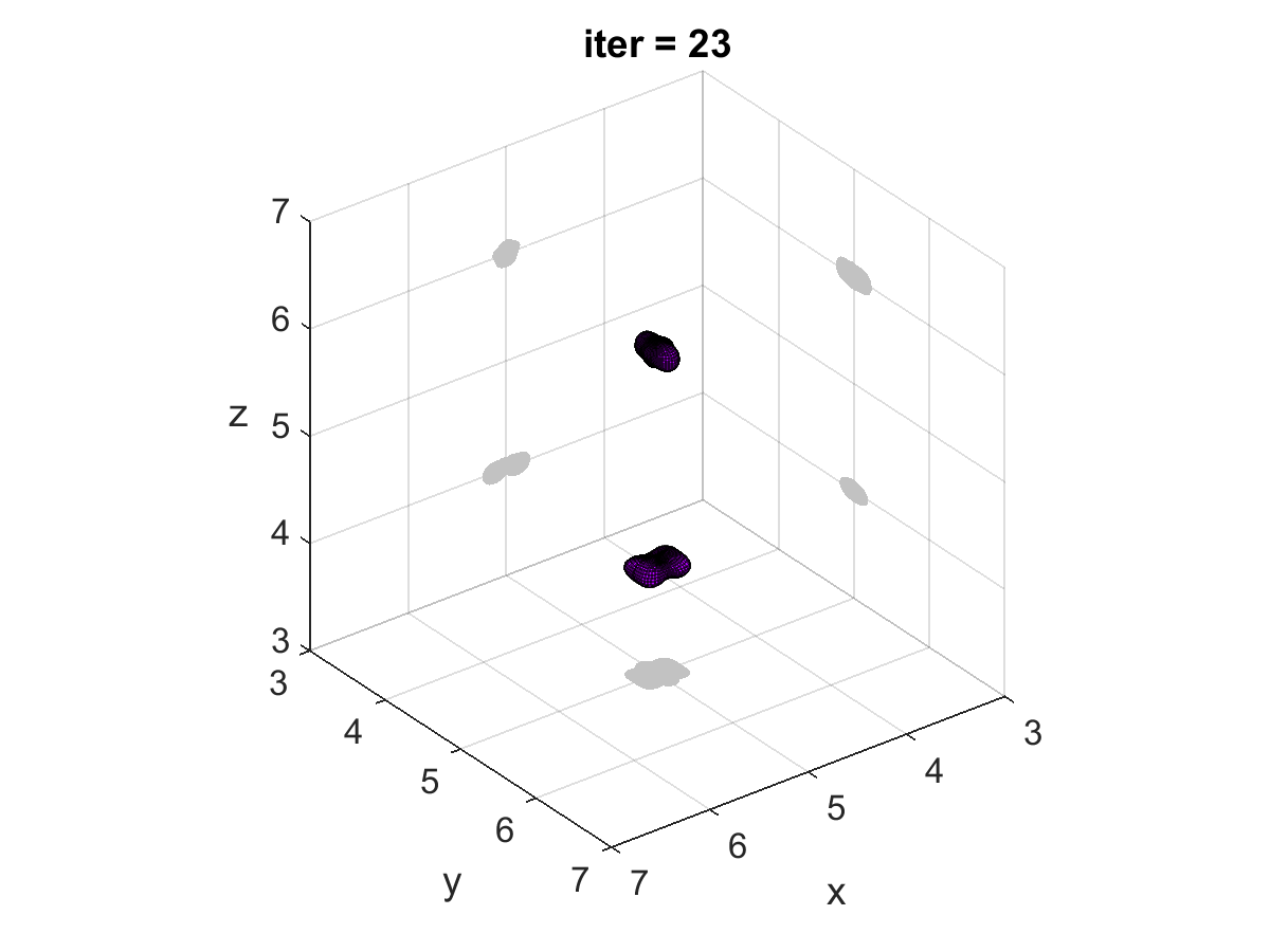
with θ∈[0,π]\theta\in[0,\pi], ϕ∈[0,2​π]\phi\in[0,2\pi] and rγ​(θ)=14​1+γ+1​cos⁡(2​θ)+γ+1−sin2⁡(2​θ).r_{\gamma}(\theta)=\frac{1}{4\sqrt{1+\sqrt{\gamma+1}}}\sqrt{\cos(2\theta)+\sqrt{\gamma+1-\sin^{2}(2\theta)}}. We select (cx,cy,cz)=(5,5,4)(c_{x},c_{y},c_{z})=(5,5,4) and γ=0.5\gamma=0.5. The parameter γ>0\gamma>0 determines the narrowness in the middle of the peanut shape (the closer to zero, the more constricted). Figure 7 illustrates the good performance of the hybrid algorithm, which recovers both shapes in 23 iterations for violet light (results for red light are similar in 24 iterations), see also Video 2 in the Supplementary Material.

If we replace the peanut by two spheres, we recover the three objects in 2222 iterations of the hybrid TD/IRGN method as shown in Figure 8, see also Video 3 in the Supplementary Material. Figure 9 and Video 4 illustrate convergence when the two spheres are placed asymmetrically. Notice that in this case, recovering the sphere aligned with the ellipsoid should be in principle more complicated than approximating the sphere not screened by it. However, our method overcomes the difficulty and provides an accurate description of both spheres.

(a)           (b)           (c)
Refer to captionRefer to captionRefer to caption
(d)           (e)           (f)
Refer to captionRefer to captionRefer to caption
(g)           (h)           (i)
Refer to captionRefer to captionRefer to caption
(j)           (k)           (l)
Refer to captionRefer to captionRefer to caption

Figure 10: Detection of three objects with different shapes and sizes using the hybrid TD/IRGN with violet light. (a) True geometry: The bean is centered at (5,5,6)(5,5,6) and described by the parameterization (77), the sphere is centered at (5,5,4)(5,5,4) with radius 0.1250.125 and the ellipsoid is centered at (5,5.5,4)(5,5.5,4) with semi-axes a=0.25a=0.25, b=0.125b=0.125 and c=0.125c=0.125. (b) Hologram. (c) Evolution of the cost functional during the optimization process. (d) Slice x=5x=5 of the topological derivative (21)-(28). (e) Initial guess Ω1\Omega_{1} defined by (20). Only one object is detected. (f) Approximate object Ω4\Omega_{4} obtained by the IRGNM. (g) Slice x=5x=5 of the topological derivative (3.2), (3.2)-(3.2) when Ω=Ω4\Omega=\Omega_{4}. Cyan contours represent the true object, whereas the approximated object section is shown in magenta. (h) Approximate object Ω5\Omega_{5} obtained from Ω4\Omega_{4} using (0). A new component is detected. (i) Slice x=5x=5 of the topological derivative when Ω=Ω5\Omega=\Omega_{5}. (j) Approximate object Ω6\Omega_{6} obtained from Ω5\Omega_{5} using (0). The third component, corresponding to the sphere, is detected. (k,l) Intermediate and final approximate objects Ω10\Omega_{10} and Ω24\Omega_{24} obtained by the IRGNM.

Finally, in Figure 10 (see also Video 5 in the supplementary material), we illustrate the performance of the hybrid algorithm in a configuration with three objects of different sizes and shapes. One of them is a bean, a non-star shaped object described by the parameterization

(5,5,6)+0.17​(A⁡(θ)​sin⁡θ​cos⁡ϕ,B⁡(θ)​sin⁡θ​sin⁡ϕ−0.3​C​(θ),cos⁡θ),(5,5,6)+0.17(A(\theta)\sin\theta\cos\phi,B(\theta)\sin\theta\sin\phi-0.3C(\theta),\cos\theta), (77)

with A⁡(θ)=0.64​(−0.1​C​(θ))A(\theta)\!=\!\sqrt{0.64(1\!-\!0.1C(\theta))}, B⁡(θ)=0.64​(−0.4​C​(θ))B(\theta)\!=\!\sqrt{0.64(1\!-\!0.4C(\theta))}, C⁡(θ)=cos⁡(π​cos⁡θ)C(\theta)=\cos(\pi\cos\theta) for θ∈[0,π]\theta\in[0,\pi], ϕ∈[0,2​π]\phi\in[0,2\pi]. The first identified object is the bean, that is closer to the screen. When the algorithm carries out a topological derivative iteration to update the number of objects, the existing approximation resembles an ellipsoid rather than a bean. After this update, only the ellipsoid is detected because is bigger than the sphere, which is not seen. Once this new component is found, the algorithm requires a new topological derivative iteration, finally determining the correct number of objects. At the 6th iteration (see panel (j)), the three objects resemble ellipsoids, but in a few iterations the true shapes are approximated with accuracy (panel (l)).

(a)           (b)           (c)
Refer to captionRefer to captionRefer to caption
(d)           (e)           (f)
Refer to captionRefer to captionRefer to caption
(g)           (h)           (i)
Refer to captionRefer to captionRefer to caption
(j)           (k)           (l)
Refer to captionRefer to captionRefer to caption

Figure 11: Performance of the hybrid TD/IRGN algorithm for different configurations of scatterers when only 121121 detectors are placed on the screen. First column: true geometries. Second column: final reconstructions. Third column: evolution of the cost functional.

Remarkably, the quality of the previous approximations is maintained when reducing drastically the number of detectors, in agreement with the observations made in [13]. Let us consider a much coarser detector grid formed by just 121121 detectors located at the points 𝐱k​ℓ=(k,ℓ,10){\bf x}_{k\ell}=(k,\ell,10), k,ℓ=0,…,10k,\ell=0,\dots,10. Figure 11 shows the results obtained for different sets of scatterers using violet light. Comparing Figure 11(b,e,h,k) with Figure 6(e), Figure 7(l), Figure 9(c) and Figure 10(l), respectively, we observe that the quality of the approximations is similar.

6 Numerical solution of boundary value and linearized problems

The optimization techniques to address the inverse holography problem described in Sections 3-5 rely on the availability of adequate solvers for the associated forward and adjoint problems on one side, and the characterization of the Fréchet derivatives on the other. All of them can be rewritten to adopt the same mathematical structure.

6.1 Forward and adjoint fields

Expressing the total light field 𝐄\mathbf{E} in terms of transmitted 𝐄tr{\mathbf{E}}_{\rm tr}, scattered 𝐄sc{\mathbf{E}}_{\rm sc} and incident 𝐄inc{\mathbf{E}}_{\rm inc} wave fields, and the conjugate adjoint field in a similar way where 𝐏¯inc\overline{\mathbf{P}}_{\rm inc} is the solution of the conjugate adjoint problem in the whole space (28) we find

𝐄={𝐄sc+𝐄incin​ℝ3∖Ω¯,𝐄trin​Ω,𝐏¯={𝐏¯sc+𝐏¯incin​ℝ3∖Ω¯,𝐏¯trin​Ω,\displaystyle{\mathbf{E}}=\left\{\begin{array}[]{ll}{\mathbf{E}}_{\rm sc}+{\mathbf{E}}_{\rm inc}&{\rm in}\,\mathbb{R}^{3}\setminus{\overline{\Omega}},\\ {\mathbf{E}}_{\rm tr}&{\rm in}\,\Omega,\\ \end{array}\right.\qquad\overline{\mathbf{P}}=\left\{\begin{array}[]{ll}\overline{\mathbf{P}}_{\rm sc}+\overline{\mathbf{P}}_{\rm inc}&{\rm in}\,\mathbb{R}^{3}\setminus{\overline{\Omega}},\\ \overline{\mathbf{P}}_{\rm tr}&{\rm in}\,\Omega,\\ \end{array}\right.

systems (3.2) and (3.2) governing the forward and adjoint fields become

𝐜𝐮𝐫𝐥⁡(𝐜𝐮𝐫𝐥​𝐖sc)−ke2​𝐖sc=0in ℝ3∖Ω¯,𝐜𝐮𝐫𝐥⁡(𝐜𝐮𝐫𝐥​𝐖tr)−ki2​𝐖tr=0in Ω,𝐧^×𝐖tr−𝐧^×𝐖sc=𝐧^×𝐖inc,on ∂Ωβ​𝐧^×𝐜𝐮𝐫𝐥​𝐖tr−𝐧^×𝐜𝐮𝐫𝐥​𝐖sc=𝐧^×𝐜𝐮𝐫𝐥​𝐖inc,on ∂Ω,lim|𝐱|→∞​|𝐱|​|𝐜𝐮𝐫𝐥​𝐖sc×𝐱^−ı​ke​𝐖sc|=0,\displaystyle\begin{array}[]{ll}\mathbf{curl}\,(\mathbf{curl}\,\mathbf{W}_{\rm sc})-k_{e}^{2}\mathbf{W}_{\rm sc}=0&\mbox{in $\mathbb{R}^{3}\setminus\overline{\Omega}$},\\ \mathbf{curl}\,(\mathbf{curl}\,\mathbf{W}_{\rm tr})-k_{i}^{2}\mathbf{W}_{\rm tr}=0&\mbox{in $\Omega$},\\ \hat{\mathbf{n}}\times\mathbf{W}_{\rm tr}-\hat{\mathbf{n}}\times\mathbf{W}_{\rm sc}=\hat{\mathbf{n}}\times\mathbf{W}_{\rm inc},&\mbox{on $\partial\Omega$}\\ \beta\,\hat{\mathbf{n}}\times\mathbf{curl}\,\mathbf{W}_{\rm tr}-\hat{\mathbf{n}}\times\mathbf{curl}\,\mathbf{W}_{\rm sc}=\hat{\mathbf{n}}\times\mathbf{curl}\,\mathbf{W}_{\rm inc},&\mbox{on $\partial\Omega$},\\ {\rm lim}_{|\mathbf{x}|\rightarrow\infty}|\mathbf{x}|\big|\mathbf{curl}\,\mathbf{W}_{\rm sc}\times\hat{\mathbf{x}}-\imath k_{e}\mathbf{W}_{\rm sc}\big|=0,&\end{array}

for 𝐖=𝐄\mathbf{W}=\mathbf{E} or 𝐏¯.\overline{\mathbf{P}}. In principle, any solver for transmission Maxwell problems can be used.

In our setting, for scatterers whose boundary is defined by a 𝒞2{\cal C}^{2}-parameteriza- tion (in particular, by a star-shaped one) with piecewise constant refractive indexes, we use fast boundary integral/spectral codes [22, 38]. Maxwell equations are solved by a Muller type boundary integral formulation [18, 38, 50]. The parametrization is exploited to transport the integral equations into unit spheres and the system is solved by means of Galerkin schemes using tangential vector spherical harmonics of low order [38]. This approach may be faster than implementing the discrete dipole approximation [58, 59] or combing boundary element (BEM)/ finite element (FEM) in a 3D region [5, 48, 51]. Unlike these two latter methods, it is only applicable when a specific parametrization is available. Fast multipole scattering methods would also be adequate in the presence of many particles [24].

6.2 Linearized equation to correct parameterizations

The least squares problem (4.2) is minimized solving numerically equation (4.2) in Hs​(𝕊2)H^{s}(\mathbb{S}^{2}) using the conjugate gradient method with initial solution 𝝃k+1=0\boldsymbol{\xi}_{k+1}=0 and residual 10−210^{-2}. In each step of the conjugate gradient method, we must apply the operators ℐ′​(𝐪k){\cal I}^{\prime}(\mathbf{q}_{k}) and ℐ′​(𝐪k)∗{\cal I}^{\prime}(\mathbf{q}_{k})^{*} to known vectors. Applying ℐ′​(𝐪k){\cal I}^{\prime}(\mathbf{q}_{k}) to a vector 𝝃\boldsymbol{\xi} amounts to solving system (4.2). System (4.2) has the structure (6.1) with transmission data (66)-(67). The techniques mentioned in Section 6.1 can be used to solve it.

To compute numerically the adjoint (71) there are two possibilities, depending on how we evaluate the Cauchy data (𝐧^×𝐄𝒉+¯,𝐧^×𝐜𝐮𝐫𝐥​𝐄𝒉+¯)(\hat{\mathbf{n}}\times\,\overline{\mathbf{E}^{+}_{\boldsymbol{h}}},\hat{\mathbf{n}}\times\mathbf{curl}\,\overline{\mathbf{E}^{+}_{\boldsymbol{h}}}):

  • (i)

    Either we compute the data (𝐧^×𝐄𝒉+,𝐧^×𝐜𝐮𝐫𝐥​𝐄𝒉+)(\hat{\mathbf{n}}\times\,{\mathbf{E}^{+}_{\boldsymbol{h}}},\hat{\mathbf{n}}\times\mathbf{curl}\,{\mathbf{E}^{+}_{\boldsymbol{h}}}) by solving the transmission problem with the incident field 𝐄𝒉i​n​c\mathbf{E}^{inc}_{\boldsymbol{h}} as indicated above. Then we take the conjugate.

  • (ii)

    Or else, we compute the hermitian adjoint (transpose of the conjugate matrix) of the discretized approximation of the operator

    (gDgN)↦ℐ′​(𝐪ap)​𝝃\begin{pmatrix}g_{D}\\ g_{N}\end{pmatrix}\mapsto{\cal I}^{\prime}(\mathbf{q}_{\rm ap})\boldsymbol{\xi}

    that provides the vector (𝐧^×𝐄𝒉+¯,𝐧^×𝐜𝐮𝐫𝐥​𝐄𝒉+¯)(\hat{\mathbf{n}}\times\overline{\mathbf{E}^{+}_{\boldsymbol{h}}},\hat{\mathbf{n}}\times\mathbf{curl}\,\overline{\mathbf{E}^{+}_{\boldsymbol{h}}}). This is our choice. Indeed, we have

    𝒉⋅ℐ′​(𝐪ap)​𝝃=Re⁡(⟨gD,𝐧^×𝐄𝒉+¯⟩L2+⟨gN,𝐧^×𝐜𝐮𝐫𝐥​𝐄𝒉+¯⟩L2).\displaystyle\boldsymbol{h}\cdot{\cal I}^{\prime}(\mathbf{q}_{\rm ap})\boldsymbol{\xi}={\rm Re}\left(\langle g_{D},\hat{\mathbf{n}}\times\overline{\mathbf{E}^{+}_{\boldsymbol{h}}}\rangle_{L^{2}}+\langle g_{N},\hat{\mathbf{n}}\times\mathbf{curl}\,\overline{\mathbf{E}^{+}_{\boldsymbol{h}}}\rangle_{L^{2}}\right). (89)

7 Conclusions

We have proposed a fully automatic algorithm to numerically reconstruct 3D objects from the holograms they generate. The method seeks to minimize the difference when comparing the true holograms and the holograms generated by approximate objects as predicted by a Maxwell forward model of light scattering. The topological derivative of this error functional provides an initial guess of the holographied objects in the absence of a priori information, other than the ambient refractive index and the incident wave. Working with star-shaped parameterizations, we implement an iteratively regularized Gauss-Newton method to successively correct the parametrization by solving linearized problems. Automatically combined with additional topological derivative based iterations to create or destroy objects when the decrease in the error functional stagnates, this procedure yields accurate reconstructions of a variety of objects in an experimental holography setting. This scheme is quite general and can be applied to other inverse electromagnetic problems by changing the error functional, so that it is defined in terms of the adequate data. This usually requires adjusting the sources in the adjoint problems and adjusting the Fréchet derivatives.

In general ‘nonlinear least squares’ problems, gradient methods seek to deform initial domains in the direction in which some kind of derivative of the error functional is negative, so that the functional decreases. This kind of methods includes topological derivative (TD), shape derivative (SD) and level set (LS) based optimization. Instead, Gauss-Newton type methods aim to correct the current approximation by linearizing about it and solving the resulting problem. Even when no spurious solutions are introduced by these procedures, they all may suffer from stagnation in the direction of small ‘gradient’. Here, the inclusion of Tikhonov regularizing terms in Gauss-Newton methods allows for convergence avoiding this artifact. From a technical point of view, while Gauss-Newton approaches require an explicit expression for a Fréchet derivative with respect to the domain, descent methods based on TD, SD or LS rely on explicit expressions for the shape/topological derivatives. Such expressions can usually be obtained introducing auxiliary adjoint problems without the need of characterizing the Fréchet derivative. The availability of these latter characterizations allows us to implement the IRGNM considered here.

We have focused on recovering shapes assuming the refractive indexes of the objects known. To obtain both we may combine our algorithm for shape optimization with parameter optimization, as in [6] or explore bayesian techniques [15]. Moreover, this paper considers object sizes of the same or smaller order than the employed light wavelength. The design of effective methods for larger objects and for objects whose components cannot be well approximated by star-shaped descriptions will require further developments.

In principle, the algorithm we propose could be extended to other inverse electromagnetic scattering problems by adjusting the closed-form formulas for the pertinent derivatives, and also to other inverse scattering problems, provided closed-form formulas for the derivatives as well as solvers for forward/adjoint problems are available (acoustics, elastography…).

Acknowledgments

This research has been supported by MINECO grants No. MTM2017-84446-C2-1-R (AC, MLR) and TRA2016-75075-R (MLR) as well as by sabbatical funds from Fundación Caja Madrid and the Salvador de Madariaga Program PRX18/00112 (AC). T.G. Dimiduk and A. Carpio thank V.N. Manoharan for discussions of holography and the Kavli Institute Seminars at Harvard for the interdisciplinary communication environment that initiated this work. A. Carpio thanks M.P. Brenner for hospitality while visiting Harvard University and R.E. Caflisch for hospitality while visiting the Courant Institute at NYU.

Appendix A Comparison with scalar approximations

When working with an incident wave polarized in the xx or yy directions, such as 𝐄inc=(Einc,0,0)\mathbf{E}_{\rm inc}=(E_{\rm inc},0,0), Einc=eı​ke​z,E_{\rm inc}=e^{\imath k_{e}z}, a standard approximation sets the non polarized components of the electric field equal to zero and uses a scalar Helmholtz transmission problem to approximate the polarized component E1E_{1}. In this framework, the inverse problem (14) is reformulated as finding Ω\Omega such that the solution EΩE_{\Omega} of the scalar forward problem

ΔE−ke2E=0inℝ3∖Ω¯,ΔE−ki2E=0inΩ,E−=E+on∂Ω,β∂E−∂𝐧^=∂E+∂𝐧^on∂Ω,lim|𝐱|→∞​|𝐱|​|∂∂|𝐱|​(E−Einc)−ı​ke​(E−Einc)|=0,\displaystyle\begin{array}[]{l}\Delta E-k_{e}^{2}E=0\;\mbox{in}\;\mathbb{R}^{3}\setminus\overline{\Omega},\qquad\Delta E-k_{i}^{2}E=0\;\mbox{in}\;\Omega,\\ E^{-}=E^{+}\;\mbox{on}\;\partial\Omega,\qquad\beta{\partial E^{-}\over\partial\hat{\mathbf{n}}}={\partial E^{+}\over\partial\hat{\mathbf{n}}}\;\mbox{on}\;\partial\Omega,\\ {\rm lim}_{|\mathbf{x}|\rightarrow\infty}|\mathbf{x}|\big|{\partial\over\partial|\mathbf{x}|}(E-E_{\rm inc})-\imath k_{e}(E-E_{\rm inc})\big|=0,\end{array}

satisfies the equations Imeas​(𝐱j)=|EΩ​(𝐱j)|2I_{\rm meas}(\mathbf{x}_{j})=|E_{\Omega}(\mathbf{x}_{j})|^{2}, j=1,…,Nj=1,\dots,N, or is a global minimum of the functional 12​∑j=1N|Imeas​(𝐱j)−|EΩ​(𝐱j)|2|2.{1\over 2}\sum_{j=1}^{N}|I_{\rm meas}(\mathbf{x}_{j})-|E_{\Omega}(\mathbf{x}_{j})|^{2}|^{2}. A scalar version of the topological methods explained in Section 3 was implemented in [6].

This strategy may be reasonable in the presence of isolated smooth scatterers, placed far enough from the detector screen. However, it introduces a number of errors of varying magnitude:

  • •

    First, Imeas​(𝐱j)=E1​(𝐱j)2+E2​(𝐱j)2+E3​(𝐱j)3I_{\rm meas}(\mathbf{x}_{j})=E_{1}(\mathbf{x}_{j})^{2}+E_{2}(\mathbf{x}_{j})^{2}+E_{3}(\mathbf{x}_{j})^{3} where 𝐄=(E1,E2,E3)\mathbf{E}=(E_{1},E_{2},E_{3}) is the solution of the vector Maxwell system (2) for the true object Ω\Omega. The boundary conditions couple the three components of the electric field at the boundary of the object. However, if we work with well separated objects and the detectors are placed far enough from them, the value of E2​(𝐱j)2+E3​(𝐱j)2E_{2}(\mathbf{x}_{j})^{2}+E_{3}(\mathbf{x}_{j})^{2} is expected to be small.

  • •

    The topological derivative for the scalar problem in the whole space is DT​(𝐱,ℝ3)=Re⁡[(ke2−ki2)​E​Q¯]D_{T}(\mathbf{x},\mathbb{R}^{3})={\rm Re}[(k_{e}^{2}-k_{i}^{2})E\overline{Q}] where E=EincE=E_{\rm inc} and the scalar adjoint Q¯\overline{Q} is an outgoing solution of

    −ΔQ¯−ke2Q¯=∑j=1Ndjδ𝐱j,dj=2(Imeas(𝐱j)−|E(𝐱j)|2)E¯(𝐱j).\displaystyle\begin{array}[]{l}-\Delta\overline{Q}-k_{e}^{2}\overline{Q}=\sum_{j=1}^{N}d_{j}\delta_{\mathbf{x}_{j}},\quad d_{j}=2(I_{\rm meas}(\mathbf{x}_{j})-|E(\mathbf{x}_{j})|^{2})\overline{E}(\mathbf{x}_{j}).\end{array}

    Particularizing formula (21) for the vector Maxwell problem with polarized light and β=1\beta=1, we find DT​(𝐱,ℝ3)=3​ke2ki2+2​ke2​Re​[(ke2−ki2)​E​P¯1]D_{T}(\mathbf{x},\mathbb{R}^{3})={3k_{e}^{2}\over k_{i}^{2}+2k_{e}^{2}}{\rm Re}[(k_{e}^{2}-k_{i}^{2})E\overline{P}_{1}], where 𝐏=(P1,P2,P3)\mathbf{P}=(P_{1},P_{2},P_{3}) is given by (3.1). To quantify the difference between both formulas for topological derivatives, we need to relate QQ and P1P_{1}. We find a term of the form ke−2∑j=1N∇divGke∗djδ𝐱jk_{e}^{-2}\sum_{j=1}^{N}\nabla{\rm div}G_{k_{e}}*d_{j}\delta_{\mathbf{x}_{j}}, where GkeG_{k_{e}} is the Green function of the Helmholtz equation. This error term decays with the distance to the detectors.

    Indeed, conjugating system (3.1) we obtain:

    𝐜𝐮𝐫𝐥⁡(𝐜𝐮𝐫𝐥​𝐏¯)−ke2​𝐏¯=2​∑j=1N(Imeas−|𝐄inc|2)​𝐄¯inc​δ𝐱jin ℝ3,lim|𝐱|→∞​|𝐱|​|𝐜𝐮𝐫𝐥​𝐏¯×𝐱^−ı​ke​𝐏¯|=0.\displaystyle\begin{array}[]{ll}\mathbf{curl}\,(\mathbf{curl}\,\overline{\mathbf{P}})-k_{e}^{2}\overline{\mathbf{P}}=2\sum_{j=1}^{N}(I_{\rm meas}-|\mathbf{E}_{\rm inc}|^{2})\overline{\mathbf{E}}_{\rm inc}\,\delta_{\mathbf{x}_{j}}&\quad\mbox{in $\mathbb{R}^{3}$},\\[4.30554pt] {\rm lim}_{|\mathbf{x}|\rightarrow\infty}|\mathbf{x}|\big|\mathbf{curl}\,\overline{\mathbf{P}}\times\hat{\mathbf{x}}-\imath k_{e}\overline{\mathbf{P}}\big|=0.&\end{array}

    For j=1,…,Nj=1,\ldots,N, we take the divergence 𝐜𝐮𝐫𝐥⁡(𝐜𝐮𝐫𝐥​𝐏¯j)−ke2​𝐏¯j=𝐝j​δ𝐱j\mathbf{curl}\,(\mathbf{curl}\,\overline{\mathbf{P}}_{j})-k_{e}^{2}\overline{\mathbf{P}}_{j}={\mathbf{d}_{j}}\delta_{\mathbf{x}_{j}}, where 𝐝j=2​(Imeas​(𝐱j)−|𝐄⁡(𝐱j)|2)​𝐄⁡(𝐱j)¯\mathbf{d}_{j}=2(I_{\rm meas}(\mathbf{x}_{j})-|\mathbf{E}(\mathbf{x}_{j})|^{2})\overline{\mathbf{E}(\mathbf{x}_{j})}. Since div⁡(𝐜𝐮𝐫𝐥​𝐀)=0{\rm div}\,(\mathbf{curl}\,\mathbf{A})=0 for any vector 𝐀\mathbf{A}, we find div​𝐏¯j=−1ke2​div​𝐝j​δ𝐱j.{\rm div}\,{\overline{\mathbf{P}}_{j}}=-{1\over k_{e}^{2}}{\rm div}\,{\mathbf{d}}_{j}\delta_{\mathbf{x}_{j}}. Making use of the vector identity 𝐜𝐮𝐫𝐥⁡(𝐜𝐮𝐫𝐥​𝐏¯j)=∇(div​𝐏¯j)−Δ​𝐏¯j\mathbf{curl}\,(\mathbf{curl}\,\overline{\mathbf{P}}_{j})=\nabla({\rm div}\,\overline{\mathbf{P}}_{j})-\Delta{\overline{\mathbf{P}}_{j}} we have

    −Δ𝐏¯j−ke2𝐏¯j=δ𝐱j𝐝j+1ke2∇(div𝐝jδ𝐱j).\displaystyle\begin{array}[]{r}-\Delta{\overline{\mathbf{P}}_{j}}-k_{e}^{2}{\overline{\mathbf{P}}_{j}}=\delta_{\mathbf{x}_{j}}{\mathbf{d}}_{j}+{1\over k_{e}^{2}}\nabla({\rm div}\,{\mathbf{d}}_{j}\delta_{\mathbf{x}_{j}}).\end{array}

    We can solve the equations by convolution with the Green function of Helmholtz equation:

    𝐏¯j=Gke∗𝐝j​δ𝐱j+1ke2​Gke∗∇(div​𝐝j​δ𝐱j).\displaystyle\begin{array}[]{r}\overline{\mathbf{P}}_{j}=G_{k_{e}}*{\mathbf{d}}_{j}\delta_{\mathbf{x}_{j}}+{1\over k_{e}^{2}}G_{k_{e}}*\nabla({\rm div}\,{\mathbf{d}}_{j}\delta_{\mathbf{x}_{j}}).\end{array}

    This expression quantifies the difference between the Green function of Maxwell equation and Green functions of Helmholtz equations. Indeed, notice that the right hand side can be rewritten as Gke∗𝐝j​δ𝐱j+1ke2​Gke∗[𝐜𝐮𝐫𝐥​𝐜𝐮𝐫𝐥​𝐝j​δ𝐱j+Δ​𝐝j​δ𝐱j].G_{k_{e}}*{\mathbf{d}}_{j}\delta_{\mathbf{x}_{j}}+{1\over k_{e}^{2}}G_{k_{e}}*[\mathbf{curl}\,\mathbf{curl}\,{\mathbf{d}}_{j}\delta_{\mathbf{x}_{j}}+\Delta{\mathbf{d}}_{j}\delta_{\mathbf{x}_{j}}]. Interchanging the derivatives in the convolution we find:

    𝐏¯j​(𝐱)=1ke2​𝐜𝐮𝐫𝐥​𝐜𝐮𝐫𝐥​Gke​(𝐱−𝐱j)​𝐝j​(𝐱j).\displaystyle\begin{array}[]{r}\overline{\mathbf{P}}_{j}(\mathbf{x})={1\over k_{e}^{2}}\mathbf{curl}\,\mathbf{curl}\,G_{k_{e}}(\mathbf{x}-\mathbf{x}_{j}){\mathbf{d}}_{j}(\mathbf{x}_{j}).\end{array}

    for 𝐱≠𝐱j\mathbf{x}\neq\mathbf{x}_{j}. Summing over jj, this implies that formula (28) for the adjoint holds pointwise as long as we do not reach the screen where the hologram is recorded.

  • •

    When we consider the topological derivatives in the presence of approximated objects Ωap≠∅\Omega_{\rm ap}\neq\emptyset, the differences between the vector and the scalar approach increase, since the expression for the topological derivative (3.2) becomes discontinuous across the boundary and the coupling of the field components at the boundary in (3.2) and (3.2) produces nonzero components for the forward and adjoint fields.

Appendix B Fréchet, shape and topological derivatives for holography

In this section we justify the formulas for the Fréchet, shape and topological derivatives for the hologram and the cost functional (15) employed throughout the paper.

Given an object Ω⊂ℝ3\Omega\subset\mathbb{R}^{3} with boundary Γ=∂Ω\Gamma=\partial\Omega, we consider variations of Ω\Omega along vector fields 𝝃.\boldsymbol{\xi}. For τ>0\tau>0, we introduce the family of deformations

φτ​𝝃(𝐱)=𝐱+τ𝝃(𝐱),𝐱∈ℝ3,\displaystyle\begin{array}[]{l}\varphi_{\tau\boldsymbol{\xi}}(\mathbf{x})=\mathbf{x}+\tau\boldsymbol{\xi}(\mathbf{x}),\quad\mathbf{x}\in\mathbb{R}^{3},\end{array}

and consider the deformed domains φτ​𝝃​(Ω)=Ωτ​𝝃.\varphi_{\tau\boldsymbol{\xi}}(\Omega)=\Omega_{\tau\boldsymbol{\xi}}. Let us quantify first the variations of the hologram under such deformations.

B.1 Fréchet derivative of the hologram

The Fréchet derivative extends the concept of differential to general spaces of infinite dimension. Given two Banach spaces XX, YY and a function ℱ:D⁡(ℱ)⊂X⟶Y{\cal F}:D({\cal F})\subset X\longrightarrow Y, its Fréchet derivative ℱ′:X⟶Y{\cal F}^{\prime}:X\longrightarrow Y is a linear bounded operator satisfying ℱ⁡(x+ξ)=ℱ⁡(x)+ℱ′​(x)​ξ+o⁡(ξ){\cal F}(x+\xi)={\cal F}(x)+{\cal F}^{\prime}(x)\xi+o(\xi) for ξ∈X\xi\in X as ‖ξ‖X→0\|\xi\|_{X}\rightarrow 0, for any x∈Xx\in X. In other words, it satisfies lim‖ξ‖X→0​‖ℱ⁡(x+ξ)−ℱ⁡(x)−ℱ′​(x)​ξ‖Y‖ξ‖X=0.{\rm lim}_{\|\xi\|_{X}\rightarrow 0}{\|{\cal F}(x+\xi)-{\cal F}(x)-{\cal F}^{\prime}(x)\xi\|_{Y}\over\|\xi\|_{X}}=0. It is related to the directional Gateaux derivative

Dξ​ℱ​(x)=limτ→0​ℱ⁡(x+τ​ξ)−ℱ⁡(x)τ\displaystyle\begin{array}[]{l}D_{\xi}{\cal F}(x)={\rm lim}_{\tau\rightarrow 0}{{\cal F}(x+\tau\xi)-{\cal F}(x)\over\tau}\end{array}

by ℱ′​(x)​ξ=Dξ​ℱ​(x).{\cal F}^{\prime}(x)\xi=D_{\xi}{\cal F}(x).

Let us introduce the operator that maps the deformation of the object boundary to the solution of the forward problem evaluated at the detectors:

ℱ:D⁡(ℱ)⊂Ck​(Γ,ℝ3)⟶ℳN×3​(ℂ)𝝃⟶(𝐄Ω𝝃​(𝐱1),…,𝐄Ω𝝃​(𝐱N))t,\displaystyle\begin{array}[]{ll}{\cal F}:&D({\cal F})\subset C^{k}(\Gamma,\mathbb{R}^{3})\longrightarrow{\cal M}_{N\times 3}(\mathbb{C})\\ &{\boldsymbol{\xi}}\longrightarrow(\mathbf{E}_{\Omega_{\boldsymbol{\xi}}}(\mathbf{x}_{1}),\ldots,\mathbf{E}_{\Omega_{\boldsymbol{\xi}}}(\mathbf{x}_{N}))^{t},\end{array}

where k≥2k\geq 2, 𝐄Ω𝝃{\mathbf{E}}_{\Omega_{\boldsymbol{\xi}}} is the solution of (2) with Ω=Ω𝝃,\Omega={\Omega_{\boldsymbol{\xi}}}, 𝐱j\mathbf{x}_{j}, j=1,…,N,j=1,\ldots,N, are detectors placed on a screen. Then, we can write the corresponding hologram as ℐ​(𝝃)j=|𝐄Ω𝝃​(𝐱j)|2=ℱ​(𝝃)j⋅ℱ​(𝝃)j¯,{\cal I}({\boldsymbol{\xi}})_{j}=|\mathbf{E}_{\Omega_{\boldsymbol{\xi}}}(\mathbf{x}_{j})|^{2}={\cal F}({\boldsymbol{\xi}})_{j}\cdot\overline{{\cal F}({\boldsymbol{\xi}})_{j}}, j=1,…,N.j=1,\ldots,N.

Theorem 1.The Fréchet derivative of the operator ℐ⁡(𝛏){\cal I}({\boldsymbol{\xi}}) and its adjoint operator are given by (59) and (71), respectively.

Proof. The Gateaux derivative 𝐄˙\dot{\mathbf{E}} of the solution of (2) in the direction 𝝃\boldsymbol{\xi} is characterized as the solution of (4.2) in [12], Theorem 6.6. This provides the Fréchet derivative of the operator ℱ{\cal F} defined by (B.1). Then,

ℐ′​(0)​𝝃=2​(Re⁡[ℱ​(0)j¯⋅(ℱ′​(0)​𝝃)j])j=1N=2​(Re⁡[𝐄Ω𝝃​(𝐱j)¯⋅𝐄˙​(𝐱j)])j=1N.\displaystyle\begin{array}[]{l}{\cal I}^{\prime}(0)\boldsymbol{\xi}=2\left({\rm Re}[\overline{{\cal F}(0)_{j}}\cdot({\cal F}^{\prime}(0)\boldsymbol{\xi})_{j}]\right)_{j=1}^{N}=2\left({\rm Re}[\overline{\mathbf{E}_{\Omega_{\boldsymbol{\xi}}}(\mathbf{x}_{j})}\cdot\dot{\mathbf{E}}(\mathbf{x}_{j})]\right)_{j=1}^{N}.\end{array}

We deduce that

ℐ′∗​(0)​𝒉=2​ℱ′∗​(0)​ℱ⁡(0)¯​𝒉,{{\cal I}^{\prime}}^{*}(0)\boldsymbol{h}=2{{\cal F}^{\prime}}^{*}(0)\overline{{\cal F}(0)}\boldsymbol{h},

where ℱ′∗​(0){{\cal F}^{\prime}}^{*}(0) is characterized in [38], Proposition 6. The only difference with respect to the use of full measurements (phase+intensity) [38] is the multiplication of the incident adjoint field by 2​𝒉2\boldsymbol{h}. □\square

Using the same formula we get similar results inspired by [33, Eq. (1.3)] for the scalar case.

Theorem 1bis. Using the scalar approximation for polarized waves, the Fréchet derivative of the operator ℐ⁡(𝛏){\cal I}({\boldsymbol{\xi}}) is given by

ℐ′​(𝐪ap)​𝝃=(2​Re​[EΩap​(𝐱1)¯​E˙​(𝐱1)]2​Re​[EΩap​(𝐱N)¯​E˙​(𝐱N)]),\displaystyle{\cal I}^{\prime}(\mathbf{q}_{\rm ap})\boldsymbol{\xi}=\begin{pmatrix}2{\rm Re}\left[\overline{E_{\Omega_{\rm ap}}(\mathbf{x}_{1})}\dot{E}(\mathbf{x}_{1})\right]\\ \vdots\\ 2{\rm Re}\left[\overline{E_{\Omega_{\rm ap}}(\mathbf{x}_{N})}\dot{E}(\mathbf{x}_{N})\right]\end{pmatrix},

where E˙\dot{E} is the solution of

ΔE˙−ke2E˙=0inℝ3∖Ω¯,ΔE˙−ki2E˙=0inΩ,E˙+−E˙−=gDon∂Ω,∂E˙+∂𝐧^−β∂E˙−∂𝐧^=gNon∂Ω,lim|𝐱|→∞​|𝐱|​|∂∂|𝐱|​E˙−ı​ke​E˙|=0,\displaystyle\begin{array}[]{l}\Delta\dot{E}-k_{e}^{2}\dot{E}=0\;\mbox{in}\;\mathbb{R}^{3}\setminus\overline{\Omega},\qquad\Delta\dot{E}-k_{i}^{2}\dot{E}=0\;\mbox{in}\;\Omega,\\ \dot{E}^{+}-\dot{E}^{-}=g_{D}\;\mbox{on}\;\partial\Omega,\qquad{\partial\dot{E}^{+}\over\partial\hat{\mathbf{n}}}-\beta{\partial\dot{E}^{-}\over\partial\hat{\mathbf{n}}}=g_{N}\;\mbox{on}\;\partial\Omega,\\ {\rm lim}_{|\mathbf{x}|\rightarrow\infty}|\mathbf{x}|\big|{\partial\over\partial|\mathbf{x}|}\dot{E}-\imath k_{e}\dot{E}\big|=0,\end{array}

with object Ω=Ωap\Omega=\Omega_{\rm ap} and transmission data

gD=−(𝝃⋅𝐧^)​(∂E+∂𝐧^−∂E−∂𝐧^),\displaystyle g_{D}=-({\boldsymbol{\xi}}\cdot{\hat{\mathbf{n}}})\left({\partial{E}^{+}\over\partial\hat{\mathbf{n}}}-{\partial{E}^{-}\over\partial\hat{\mathbf{n}}}\right),
gN=(𝝃⋅𝐧^)(ke2E+−ki2βE−)+div∂Ω((𝝃⋅𝐧^)(∇E+−β∇E−)),\displaystyle g_{N}=({\boldsymbol{\xi}}\cdot{\hat{\mathbf{n}}})\left(k_{e}^{2}E^{+}-k_{i}^{2}\beta\,\ E^{-}\right)+{\rm div}_{\partial\Omega}\left(({\boldsymbol{\xi}}\cdot{\hat{\mathbf{n}}})(\nabla E^{+}-\beta\nabla E^{-})\right),

E=EΩapE=E_{\Omega_{\rm ap}} being the solution of (A) with Ω=Ωap\Omega=\Omega_{\rm ap} and 𝐧^\hat{\mathbf{n}} the outer unit normal. The L2L^{2}-adjoint operator is defined by

𝝃∗(𝐱^)=r∗(𝐱^)𝐱^=ℐ′(𝐪ap)|L2∗𝒉,r∗=𝐱^⋅ℐ′(𝐪ap)|L2∗𝒉=r2apRe[−(1−β−1)∂E𝒉+¯∂𝐧^⋅∂E+¯∂𝐧^−(ke2−βki2)E𝒉+¯⋅E+¯+(1−β)∇∂ΩE𝒉+¯⋅∇∂ΩE+¯]∘𝐪ap,\displaystyle\begin{aligned} &\boldsymbol{\xi}^{*}(\hat{\mathbf{x}})=r^{*}(\hat{\mathbf{x}})\hat{\mathbf{x}}={\cal I}^{\prime}(\mathbf{q}_{\rm ap})_{|L^{2}}^{*}\boldsymbol{h},\\ r^{*}=\hat{\mathbf{x}}\cdot{\cal I}^{\prime}(\mathbf{q}_{\rm ap})_{|L^{2}}^{*}\boldsymbol{h}=&\;r^{2}_{\rm ap}{\rm Re}\Big[-(1-\beta^{-1}){\partial\overline{E^{+}_{\boldsymbol{h}}}\over\partial\hat{\mathbf{n}}}\cdot{\partial\overline{E^{+}}\over\partial\hat{\mathbf{n}}}-({k_{e}^{2}}-{\beta k_{i}^{2}})\overline{E^{+}_{\boldsymbol{h}}}\cdot\overline{E^{+}}\\ &\hskip 28.45274pt+(1-\beta){\nabla}_{\partial\Omega}\overline{E^{+}_{\boldsymbol{h}}}\,\cdot\,{\nabla}_{\partial\Omega}\overline{E^{+}}\Big]\circ\mathbf{q}_{\rm ap},\end{aligned}

where E𝒉+{E^{+}_{\boldsymbol{h}}} is the solution of the transmission problem (A) with object Ω=Ωap\Omega=\Omega_{\rm ap} and incident field

E𝒉i​n​c​(𝐱)=∑j=1Nei​ke​|𝐱−𝐱j|4​π​|𝐱−𝐱j|​2​𝒉​(𝐱j)​EΩap​(𝐱j)¯.E^{inc}_{\boldsymbol{h}}(\mathbf{x})=\sum_{j=1}^{N}\frac{e^{ik_{e}|\mathbf{x}-\mathbf{x}_{j}|}}{4\pi|\mathbf{x}-\mathbf{x}_{j}|}2\boldsymbol{h}(\mathbf{x}_{j})\overline{E_{\Omega_{\rm ap}}(\mathbf{x}_{j})}.

B.2 Shape derivative of the cost functional

When instead of the hologram we differentiate the cost functional (15) with respect to deformations along vector fields, we obtain the so-called shape derivative. Let us fix a vector field 𝝃\boldsymbol{\xi}. For any region ℛ{\cal R}, the deformed domain φτ​(ℛ)\varphi_{\tau}({\cal R}) is the image of ℛ{\cal R} by the deformation (B). Evaluating J{J} on the deformed regions, we obtain a scalar function J⁡(τ)=J⁡(φτ​(ℛ))J(\tau)={J}(\varphi_{\tau}({\cal R})) of the deformation parameter τ\tau, which can be differentiated with respect to it. The shape derivative along the vector field 𝝃\boldsymbol{\xi} is precisely this derivative:

⟨D​J​(ℛ),𝝃⟩:=dd​τ​J​(φτ​(ℛ))|τ=0.\displaystyle\langle D{J}({\cal R}),\boldsymbol{\xi}\rangle:=\frac{d}{d\tau}\,{J}(\varphi_{\tau}({\cal R}))\bigg|_{\tau=0}. (108)

Theorem 2. Let us assume that Ω\Omega is a C2C^{2} domain and the coefficients ke,ki,βk_{e},k_{i},\beta are piecewise constant in the different components. Then the shape derivative ⟨D​J​(ℝ3∖Ω¯),𝛏⟩\langle DJ(\mathbb{R}^{3}\setminus\overline{\Omega}),\boldsymbol{\xi}\rangle of functional (15) is given by:

Re[∫∂Ω(𝝃⋅𝐧^)(ke2−ki2β)[(𝐧^×𝐄−)⋅(𝐧^×𝐏¯−)+ki2​βke2(𝐧^⋅𝐄−)⋅(𝐧^⋅𝐏¯−)]−(𝝃⋅𝐧^)(−β)[β(𝐧^×𝐜𝐮𝐫𝐥𝐄−)⋅(𝐧^×𝐜𝐮𝐫𝐥𝐏¯−)+(𝐧^⋅𝐜𝐮𝐫𝐥𝐄−)⋅(𝐧^⋅𝐜𝐮𝐫𝐥𝐏¯−)]]dS,\displaystyle\begin{array}[]{l}{\rm Re}\bigg[\int_{\partial\Omega}(\boldsymbol{\xi}\!\cdot\!\hat{\mathbf{n}})(k_{e}^{2}\!-\!k_{i}^{2}\beta)\left[(\hat{\mathbf{n}}\!\times\!\mathbf{E}^{-})\!\cdot\!(\hat{\mathbf{n}}\!\times\!\overline{\mathbf{P}}^{-})\!+\!{k_{i}^{2}\beta\over k_{e}^{2}}(\hat{\mathbf{n}}\!\cdot\!\mathbf{E}^{-})\!\cdot\!(\hat{\mathbf{n}}\!\cdot\!\overline{\mathbf{P}}^{-})\right]\\ \ -(\boldsymbol{\xi}\!\cdot\!\hat{\mathbf{n}})(1\!-\!\beta)\left[\beta(\hat{\mathbf{n}}\!\times\!\mathbf{curl}\,\mathbf{E}^{-})\!\cdot\!(\hat{\mathbf{n}}\!\times\!\mathbf{curl}\,\overline{\mathbf{P}}^{-})\!+\!(\hat{\mathbf{n}}\!\cdot\!\mathbf{curl}\,\mathbf{E}^{-})\!\cdot\!(\hat{\mathbf{n}}\!\cdot\!\mathbf{curl}\,\overline{\mathbf{P}}^{-})\right]\bigg]dS,\end{array}

where 𝐄\mathbf{E} and 𝐏¯\overline{\mathbf{P}} are the solutions of the forward and conjugate adjoint problems (3.2) and (3.2).

Proof. Given the vector field 𝝃\boldsymbol{\xi}, we must evaluate (108). Differentiating with respect to τ\tau the function J⁡(ℝ3∖ϕτ​(Ω)¯)J(\mathbb{R}^{3}\setminus\overline{\phi_{\tau}(\Omega)}) with JJ given by (15) we find a vector version of the scalar formula in [6]:

d​J​(ℝ3∖ϕτ​(Ω)¯)d​τ=Re⁡[∑j=1N2​(|𝐄τ​(𝐱j)|2−Imeas​(𝐱j))​𝐄¯τ​(𝐱j)⋅d​𝐄τd​τ​(𝐱j)],\displaystyle\begin{array}[]{l}{dJ(\mathbb{R}^{3}\setminus\overline{\phi_{\tau}(\Omega)})\over d\tau}={\rm Re}\left[\sum_{j=1}^{N}2\left(|\mathbf{E}_{\tau}(\mathbf{x}_{j})|^{2}-I_{\rm meas}(\mathbf{x}_{j})\right)\overline{\mathbf{E}}_{\tau}(\mathbf{x}_{j})\cdot{d\mathbf{E}_{\tau}\over d\tau}(\mathbf{x}_{j})\right],\end{array}

where 𝐄τ\mathbf{E}_{\tau} is a solution of the forward problem (3.2) with object Ωτ=φτ​(Ω).\Omega_{\tau}=\varphi_{\tau}(\Omega). Evaluating at τ=0\tau=0, we obtain

d​J​(ℝ3∖ϕτ​(Ω)¯)d​τ|τ=0=Re⁡[∑j=1N2​(|𝐄⁡(𝐱j)|2−Imeas​(𝐱j))​𝐄¯​(𝐱j)⋅𝐄˙​(𝐱j)],\displaystyle\begin{array}[]{l}{dJ(\mathbb{R}^{3}\setminus\overline{\phi_{\tau}(\Omega)})\over d\tau}\Big|_{\tau=0}={\rm Re}\left[\sum_{j=1}^{N}2\left(|\mathbf{E}(\mathbf{x}_{j})|^{2}-I_{\rm meas}(\mathbf{x}_{j})\right)\overline{\mathbf{E}}(\mathbf{x}_{j})\cdot\dot{\mathbf{E}}(\mathbf{x}_{j})\right],\end{array}

since 𝐄0=𝐄\mathbf{E}_{0}=\mathbf{E} is the solution of (3.2) with object Ω\Omega.

We set 𝐄˙=d​𝐄τd​τ|τ=0\dot{\mathbf{E}}={d\mathbf{E}_{\tau}\over d\tau}\Big|_{\tau=0}, which is the Gateaux derivative in the direction 𝝃\boldsymbol{\xi} of the solutions of the forward problems (3.2) with deformed domains Ωτ\Omega_{\tau}. For the transmission Maxwell system it is characterized as the solution of (4.2), see [12]. Then, elliptic regularity and Sobolev’s embeddings ensure continuity of the solution and continuity of derivatives away from the interface ∂Ω\partial\Omega [23, 25, 51]. Therefore, we can evaluate it at the detectors.

We rewrite the right hand side in identity (B.2) as follows. Integrating the equations for the adjoint field and using Green’s formula we obtain the identities:

∫Ω(β​𝐜𝐮𝐫𝐥​𝐜𝐮𝐫𝐥​𝐏¯−β​ki2​𝐏¯)⋅𝐄˙−∫∂Ωβ​𝐧^×𝐜𝐮𝐫𝐥​𝐏¯−⋅𝐄˙−=∫Ω(β​𝐜𝐮𝐫𝐥​𝐜𝐮𝐫𝐥​𝐄˙−β​ki2​𝐄˙)⋅𝐏¯−∫∂Ωβ​𝐧^×𝐜𝐮𝐫𝐥​𝐄˙−⋅𝐏¯−\displaystyle\hskip-28.45274pt\begin{array}[]{l}\int_{\Omega}(\beta\,\mathbf{curl}\,\mathbf{curl}\,\overline{\mathbf{P}}-\beta\,k_{i}^{2}\overline{\mathbf{P}})\cdot\dot{\mathbf{E}}-\int_{\partial\Omega}\beta\ \hat{\mathbf{n}}\times\mathbf{curl}\,\overline{\mathbf{P}}^{-}\cdot\dot{\mathbf{E}}^{-}\\ =\int_{\Omega}(\beta\,\mathbf{curl}\,\mathbf{curl}\,\dot{\mathbf{E}}-\beta\,k_{i}^{2}\dot{\mathbf{E}})\cdot\overline{\mathbf{P}}-\int_{\partial\Omega}\beta\,\hat{\mathbf{n}}\times\mathbf{curl}\,\dot{\mathbf{E}}^{-}\cdot\overline{\mathbf{P}}^{-}\end{array}

and

∫BR∖Ω¯(𝐜𝐮𝐫𝐥​𝐜𝐮𝐫𝐥​𝐏¯−ke2​𝐏¯)⋅𝐄˙+∫∂Ω𝐧^×𝐜𝐮𝐫𝐥​𝐏¯+⋅𝐄˙+−∫∂BRı​ke​Lke​(𝐧^R×𝐏¯)⋅𝐄˙=∫BR∖Ω¯(𝐜𝐮𝐫𝐥​𝐜𝐮𝐫𝐥​𝐄˙−ke2​𝐄˙)⋅𝐏¯+∫∂Ω𝐧^×𝐜𝐮𝐫𝐥​𝐄˙+⋅𝐏¯+−∫∂BRı​ke​Lke​(𝐧^R×𝐄˙)⋅𝐏¯.\displaystyle\begin{array}[]{l}\int_{B_{R}\setminus\overline{\Omega}}(\mathbf{curl}\,\mathbf{curl}\,\overline{\mathbf{P}}\!-\!k_{e}^{2}\overline{\mathbf{P}})\!\cdot\!\dot{\mathbf{E}}\!+\!\int_{\partial\Omega}\hskip-2.84526pt\hat{\mathbf{n}}\!\times\!\mathbf{curl}\,\overline{\mathbf{P}}^{+}\!\!\cdot\!\dot{\mathbf{E}}^{+}\!\!-\!\!\int_{\partial B_{R}}\hskip-7.11317pt\imath k_{e}L_{k_{e}}\!(\hat{\mathbf{n}}_{R}\!\times\!\overline{\mathbf{P}})\!\cdot\!\dot{\mathbf{E}}\\ =\int_{B_{R}\setminus{\overline{\Omega}}}(\mathbf{curl}\,\mathbf{curl}\,\dot{\mathbf{E}}\!-\!k_{e}^{2}\dot{\mathbf{E}})\!\cdot\!\overline{\mathbf{P}}\!+\!\int_{\partial\Omega}\hskip-2.84526pt\hat{\mathbf{n}}\!\times\!\mathbf{curl}\,\dot{\mathbf{E}}^{+}\!\!\cdot\!\overline{\mathbf{P}}^{+}\!\!-\!\!\int_{\partial B_{R}}\hskip-7.11317pt\imath k_{e}L_{k_{e}}\!(\hat{\mathbf{n}}_{R}\!\times\!\dot{\mathbf{E}})\!\cdot\!\overline{\mathbf{P}}.\end{array}

Here, BR=B⁡(𝟎,R)B_{R}=B(\mathbf{0},R) is a sphere with radius RR large enough to contain the objects and detectors and LkeL_{k_{e}} stands for the Dirichlet to Neumann operator for Maxwell equations [49, Chapter 10]. To be able to use the transmission boundary conditions for 𝐄˙\dot{\mathbf{E}} we combine (B.2)-(B.2) to get:

∑j=1N2​(|𝐄⁡(𝐱j)|2−Imeas​(𝐱j))​𝐄¯​(𝐱j)⋅𝐄˙​(𝐱j)=−∫∂Ω𝐧^×(𝐜𝐮𝐫𝐥𝐄˙+−β𝐜𝐮𝐫𝐥𝐄˙−)⋅𝐏¯−−∫∂Ω𝐧^×𝐜𝐮𝐫𝐥𝐄˙+⋅(𝐏¯+−𝐏¯−)+∫∂Ωβ𝐧^×𝐜𝐮𝐫𝐥𝐏¯−⋅(𝐄˙+−𝐄˙−)−∫∂Ω𝐧^×(β𝐜𝐮𝐫𝐥𝐏¯−−𝐜𝐮𝐫𝐥𝐏¯+)⋅𝐄˙+.\displaystyle\hskip-28.45274pt\begin{array}[]{l}\sum_{j=1}^{N}2\left(|\mathbf{E}(\mathbf{x}_{j})|^{2}-I_{\rm meas}(\mathbf{x}_{j})\right)\overline{\mathbf{E}}(\mathbf{x}_{j})\cdot\dot{\mathbf{E}}(\mathbf{x}_{j})=\\ -\int_{\partial\Omega}\hat{\mathbf{n}}\times(\mathbf{curl}\,\dot{\mathbf{E}}^{+}-\beta\,\mathbf{curl}\,\dot{\mathbf{E}}^{-})\cdot\overline{\mathbf{P}}^{-}-\int_{\partial\Omega}\hat{\mathbf{n}}\times\mathbf{curl}\,\dot{\mathbf{E}}^{+}\cdot(\overline{\mathbf{P}}^{+}-\overline{\mathbf{P}}^{-})\\ +\int_{\partial\Omega}\beta\,\hat{\mathbf{n}}\times\mathbf{curl}\,\overline{\mathbf{P}}^{-}\cdot(\dot{\mathbf{E}}^{+}-\dot{\mathbf{E}}^{-})-\int_{\partial\Omega}\hat{\mathbf{n}}\times(\beta\,\mathbf{curl}\,\overline{\mathbf{P}}^{-}-\mathbf{curl}\,\overline{\mathbf{P}}^{+})\cdot\dot{\mathbf{E}}^{+}.\end{array}

Following [36], we analyze the boundary terms in this identity using the boundary conditions satisfied by 𝐄˙\dot{\mathbf{E}}, 𝐄\mathbf{E}, 𝐏¯\overline{\mathbf{P}}, together with classical vector identities and differential calculus relations on surfaces [51], to finally obtain the desired expression using (B.2), see [36] for details. □\square

This Theorem is stated for piecewise constant coefficients and C2C^{2} domains. However, piecewise C1C^{1} coefficients and Lipschitz domains suffice [14, 29, 51].

Shape derivatives can be exploited to optimize the cost functional (15) since they provide vector fields 𝝃\boldsymbol{\xi} to deform an initial guess Ωap\Omega_{\rm ap} in such a way that the cost functional decreases. The vector field 𝝃\boldsymbol{\xi} is selected to ensure that the shape derivative of (15) is negative. The process can be repeated, generating a sequence of reconstructions along which the cost functional diminishes.

When β=1\beta=1, the shape derivative of the cost functional (15) at the scatterer Ωap\Omega_{\rm ap} is given by

⟨DJ(ℝ3∖Ω¯ap),𝝃⟩=Re[∫∂Ωap(𝝃⋅𝐧^)(ke2−ki2)((𝐧^×𝐄−)⋅(𝐧^×𝐏¯−)+ki2ke2(𝐧^⋅𝐄−)⋅(𝐧^⋅𝐏¯−))dS]\displaystyle\begin{array}[]{r}\langle DJ(\mathbb{R}^{3}\setminus\overline{\Omega}_{\rm ap}),\boldsymbol{\xi}\rangle={\rm Re}\Big[\int_{\partial\Omega_{\rm ap}}(\boldsymbol{\xi}\cdot\hat{\mathbf{n}})(k_{e}^{2}-k_{i}^{2})\Big((\hat{\mathbf{n}}\times\mathbf{E}^{-})\cdot(\hat{\mathbf{n}}\times\overline{\mathbf{P}}^{-})\\ +{k_{i}^{2}\over k_{e}^{2}}(\hat{\mathbf{n}}\cdot\mathbf{E}^{-})\cdot(\hat{\mathbf{n}}\cdot\overline{\mathbf{P}}^{-})\Big)dS\Big]\end{array}

where 𝐄\mathbf{E} and 𝐏\mathbf{P} are the solutions of the forward and adjoint problems (3.2) and (3.2) with object Ωap\Omega_{\rm ap}. Choosing 𝝃=ξn​𝐧^\boldsymbol{\xi}=\xi_{n}\hat{\mathbf{n}}, 𝐧^\hat{\mathbf{n}} being the unit normal vector on ∂Ωap,\partial\Omega_{\rm ap}, with

ξn=𝝃⋅𝐧^=(ki2−ke2)​Re​[(𝐧^×𝐄−)⋅(𝐧^×𝐏¯−)+ki2ke2​(𝐧^⋅𝐄−)⋅(𝐧^⋅𝐏¯−)]\displaystyle\begin{array}[]{l}\xi_{n}=\boldsymbol{\xi}\cdot\hat{\mathbf{n}}=(k_{i}^{2}-k_{e}^{2})\,{\rm Re}\Big[(\hat{\mathbf{n}}\times\mathbf{E}^{-})\cdot(\hat{\mathbf{n}}\times\overline{\mathbf{P}}^{-})+{k_{i}^{2}\over k_{e}^{2}}(\hat{\mathbf{n}}\cdot\mathbf{E}^{-})\cdot(\hat{\mathbf{n}}\cdot\overline{\mathbf{P}}^{-})\Big]\end{array}

we ensure ⟨D​J​(ℝ3∖Ω¯ap),𝝃⟩<0\langle DJ(\mathbb{R}^{3}\setminus\overline{\Omega}_{\rm ap}),\boldsymbol{\xi}\rangle<0. A new approximation is defined as

Ωnew=Ωap+τ​𝝃​(Ωap)={𝐱+τ​𝝃​(𝐱),𝐱∈Ωap}.\displaystyle\begin{array}[]{l}\Omega_{\rm new}=\Omega_{\rm ap}+\tau\boldsymbol{\xi}(\Omega_{\rm ap})=\{\mathbf{x}+\tau\boldsymbol{\xi}(\mathbf{x}),\;\mathbf{x}\in\Omega_{\rm ap}\}.\end{array}

Then, J⁡(ℝ3∖Ω¯new)<J⁡(ℝ3∖Ω¯ap)J(\mathbb{R}^{3}\setminus\overline{\Omega}_{\rm new})<J(\mathbb{R}^{3}\setminus\overline{\Omega}_{\rm ap}) for τ>0\tau>0 small.

When enforcing star-shaped parameterizations we should fit a star-shaped parametrization to the resulting object. Alternatively, we can adapt an strategy to preserve the parametrization used in [9]. We define a set of directions associated to the parametrization:

𝐕1=(1,0,0),𝐕2=(0,1,0),𝐕3=(0,0,1),𝐕n,m=𝐱|𝐱|Ynm(𝐱|𝐱|),m=−n,…,n,n=0,…,nm​a​x.\displaystyle\begin{array}[]{l}\mathbf{V}_{1}=(1,0,0),\,\mathbf{V}_{2}=(0,1,0),\mathbf{V}_{3}=(0,0,1),\\[4.30554pt] \mathbf{V}_{n,m}={\mathbf{x}\over|\mathbf{x}|}Y_{n}^{m}({\mathbf{x}\over|\mathbf{x}|}),\quad m=-n,...,n,\,n=0,...,n_{max}.\end{array}

Then, the parameters defining the star-shaped boundary of the new approximation Ωnew\Omega_{\rm new} would be:

cℓnew=cℓap−τℓ⟨DJ(ℝ3∖Ω¯ap),𝐕ℓ⟩,γn,mnew=γn,map−τn,m⟨DJ(ℝ3∖Ω¯ap),𝐕n,m⟩,\displaystyle\begin{array}[]{l}c_{\ell}^{\rm new}=c_{\ell}^{\rm ap}-\tau_{\ell}\langle DJ(\mathbb{R}^{3}\setminus\overline{\Omega}_{\rm ap}),\mathbf{V}_{\ell}\rangle,\quad\gamma_{n,m}^{\rm new}=\gamma_{n,m}^{\rm ap}-\tau_{n,m}\langle DJ(\mathbb{R}^{3}\setminus\overline{\Omega}_{\rm ap}),\mathbf{V}_{n,m}\rangle,\end{array}

with τℓ,τn,m>0\tau_{\ell},\tau_{n,m}>0 small enough. We have tested both procedures, but the approximations stagnate without converging, as it happens for the topological derivative based iterations.

B.3 Topological derivative of the cost functional

Once an explicit formula for the shape derivative of a cost functional is available, we can obtain an explicit formula for the topological derivative taking an additional limit [20]. For every 𝐱∈ℛ,\mathbf{x}\in{\cal R}, we set Bε=B⁡(𝐱,ε)B_{\varepsilon}=B({\mathbf{x}},\varepsilon) and ℛε=ℛ∖Bε¯,{\cal R}_{\varepsilon}={\cal R}\setminus\overline{B_{\varepsilon}}, we have [20]:

DT​(𝐱,ℛ)=limε→0J⁡(ℛε)−J⁡(ℛ)43​π​ε3=limε→0⟨D​J​(ℛε),𝝃⟩4​π​ε2\displaystyle D_{T}({\mathbf{x}},{\cal R})=\lim_{\varepsilon\to 0}{J({\cal R}_{\varepsilon})-J({\cal R})\over{4\over 3}\pi\varepsilon^{3}}=\lim_{\varepsilon\to 0}\frac{\langle D{J}({\cal R}_{\varepsilon}),\boldsymbol{\xi}\rangle}{4\pi\varepsilon^{2}}
=limε→0(14​π​ε2​dd​τ​J​(φτ​(ℛε))|τ=0),\displaystyle=\lim_{\varepsilon\to 0}\left(\frac{1}{4\pi\varepsilon^{2}}\,\frac{d}{d\tau}{J}(\varphi_{\tau}({\cal R}_{\varepsilon}))\bigg|_{\tau=0}\right), (134)

for every 𝐱∈ℛ\mathbf{x}\in{\cal R} 11 1 Reference [20] uses −4​π​ε2-{4\pi\varepsilon^{2}}. This changes the sign of DT​(𝐱,ℛ)D_{T}({\mathbf{x}},{\cal R}) at each point.. The vector field 𝝃\boldsymbol{\xi} is an extension to ℝ3\mathbb{R}^{3} of 𝝃=𝐧^​(𝐳),𝐳∈Γε=∂Bε​(𝐱),\boldsymbol{\xi}=\hat{\bf n}({\mathbf{z}}),\,{\mathbf{z}}\in\Gamma_{\varepsilon}=\partial B_{\varepsilon}({\mathbf{x}}), where the normal 𝐧^​(𝐳)=𝐳−𝐱|𝐳−𝐱|\hat{\bf n}({\bf z})={{\bf z}-{\bf x}\over|{\bf z}-{\bf x}|} points outside22 2 Reference [20] and later work often select the inner normal vector to the ball instead of the exterior one, setting 𝐕=−𝐧⁡(𝐳){\bf V}=-{\bf n}({\mathbf{z}}) at the boundary, which is equivalent. the ball, and vanishes out of a narrow neighborhood of ∂Bε\partial B_{\varepsilon}.

Theorem 3. Let us assume that Ω\Omega is a C2C^{2} domain and the coefficients ke,ki,βk_{e},k_{i},\beta are constant. Then the topological derivative of functional (15) in ℝ3\mathbb{R}^{3} is given by (21) with forward and adjoint fields governed by (3.1) and (3.1).

Proof. Expressions of the form (21) for cost functionals involving the full wave field were first established in [47] using asymptotic expansions. We obtain it here exploiting the relation with shape derivatives (B.3), as in [6, 8, 20, 36], To find an expression for the topological derivative in terms of adjoint and forward fields we must first evaluate the shape derivative. We set here ℛ=ℝ3{\cal R}=\mathbb{R}^{3}. By Theorem 2 in Appendix B.2, ⟨D​J​(ℝ3∖Bε¯),𝝃⟩\langle DJ(\mathbb{R}^{3}\setminus\overline{B_{\varepsilon}}),\boldsymbol{\xi}\rangle is given by

Re[∫∂Bε(ke2−ki2β)[(𝐧^ε×𝐄ε−)⋅(𝐧^ε×𝐏¯ε−)+ki2​βke2(𝐧^ε⋅𝐄ε−)⋅(𝐧^ε⋅𝐏¯ε−)]−(−β)[β(𝐧^ε×𝐜𝐮𝐫𝐥𝐄ε−)⋅(𝐧^ε×𝐜𝐮𝐫𝐥𝐏¯ε−)+(𝐧^ε⋅𝐜𝐮𝐫𝐥𝐄ε−)⋅(𝐧^ε⋅𝐜𝐮𝐫𝐥𝐏¯ε−)]]dS,\displaystyle\begin{array}[]{l}{\rm Re}\bigg[\int_{\partial B_{\varepsilon}}(k_{e}^{2}\!-\!k_{i}^{2}\beta)\left[(\hat{\mathbf{n}}_{\varepsilon}\!\times\!\mathbf{E}_{\varepsilon}^{-})\!\cdot\!(\hat{\mathbf{n}}_{\varepsilon}\!\times\!\overline{\mathbf{P}}_{\varepsilon}^{-})\!+\!{k_{i}^{2}\beta\over k_{e}^{2}}(\hat{\mathbf{n}}_{\varepsilon}\!\cdot\!\mathbf{E}_{\varepsilon}^{-})\!\cdot\!(\hat{\mathbf{n}}_{\varepsilon}\!\cdot\!\overline{\mathbf{P}}_{\varepsilon}^{-})\right]\\ -(1\!-\!\beta)\!\left[\beta(\hat{\mathbf{n}}_{\varepsilon}\!\times\!\mathbf{curl}\,\mathbf{E}_{\varepsilon}^{-})\!\cdot\!(\hat{\mathbf{n}}_{\varepsilon}\!\times\!\mathbf{curl}\,\overline{\mathbf{P}}_{\varepsilon}^{-})\!+\!(\hat{\mathbf{n}}_{\varepsilon}\!\cdot\!\mathbf{curl}\,\mathbf{E}_{\varepsilon}^{-})\!\cdot\!(\hat{\mathbf{n}}_{\varepsilon}\!\cdot\!\mathbf{curl}\,\overline{\mathbf{P}}_{\varepsilon}^{-})\right]\!\!\bigg]dS,\end{array}

where 𝐄ε\mathbf{E}_{\varepsilon} and 𝐏ε\mathbf{P}_{\varepsilon} are the solutions of the forward and adjoint problems (3.2) and (3.2) with object BεB_{\varepsilon}. These solutions admit explicit forms given by the series expansions in C. From them, we obtain the following asymptotic behaviors when |𝝌|=1|\boldsymbol{\chi}|=1 as in [6, 36]:

𝐧^ε×𝐄ε−​(𝐱+ε​𝝌)→3​(ki2​βke2+2)−1​𝝌×𝐄inc​(𝐱),𝐧^ε⋅𝐄ε−​(𝐱+ε​𝝌)→3​(ki2​βke2+2)−1​𝝌⋅𝐄inc​(𝐱),𝐧^ε×𝐜𝐮𝐫𝐥​𝐄ε−​(𝐱+ε​𝝌)→3​(1+2​β)−1​𝝌×𝐜𝐮𝐫𝐥​𝐄inc​(𝐱),𝐧^ε⋅𝐜𝐮𝐫𝐥​𝐄ε−​(𝐱+ε​𝝌)→3​(1+2​β)−1​𝝌⋅𝐜𝐮𝐫𝐥​𝐄inc​(𝐱),\displaystyle\hskip-28.45274pt\begin{array}[]{r}\hat{\mathbf{n}}_{\varepsilon}\times\mathbf{E}_{\varepsilon}^{-}(\mathbf{x}+\varepsilon\boldsymbol{\chi})\rightarrow 3\left({k_{i}^{2}\beta\over k_{e}^{2}}+2\right)^{-1}\boldsymbol{\chi}\times\mathbf{E}_{\rm inc}(\mathbf{x}),\\ \hat{\mathbf{n}}_{\varepsilon}\cdot\mathbf{E}_{\varepsilon}^{-}(\mathbf{x}+\varepsilon\boldsymbol{\chi})\rightarrow 3\left({k_{i}^{2}\beta\over k_{e}^{2}}+2\right)^{-1}\boldsymbol{\chi}\cdot\mathbf{E}_{\rm inc}(\mathbf{x}),\\ \hat{\mathbf{n}}_{\varepsilon}\times\mathbf{curl}\,\mathbf{E}_{\varepsilon}^{-}(\mathbf{x}+\varepsilon\boldsymbol{\chi})\rightarrow 3\left(1+2\beta\right)^{-1}\boldsymbol{\chi}\times\mathbf{curl}\,\mathbf{E}_{\rm inc}(\mathbf{x}),\\ \hat{\mathbf{n}}_{\varepsilon}\cdot\mathbf{curl}\,\mathbf{E}_{\varepsilon}^{-}(\mathbf{x}+\varepsilon\boldsymbol{\chi})\rightarrow 3\left(1+2\beta\right)^{-1}\boldsymbol{\chi}\cdot\mathbf{curl}\,\mathbf{E}_{\rm inc}(\mathbf{x}),\end{array}

when ε→0.\varepsilon\rightarrow 0. To justify this asymptotic behavior, we use the series expansion (159) with coefficients (C) for R=εR=\varepsilon at 𝐳=𝐱+ε​𝝌,\mathbf{z}=\mathbf{x}+\varepsilon\boldsymbol{\chi}, evaluating αn,m\alpha_{n,m},βn,m\beta_{n,m} from the series expansion of the incident wave (C). Since the spheres are centered at a point 𝐱\mathbf{x} instead of 𝟎\mathbf{0}, 𝐌n,m(1)​(ki,𝐱)\mathbf{M}_{n,m}^{(1)}(k_{i},\mathbf{x}) and 𝐍n,m(1)​(ki,𝐱)\mathbf{N}_{n,m}^{(1)}(k_{i},\mathbf{x}) are replaced by 𝐌n,m(1)​(ki,𝐳−𝐱)\mathbf{M}_{n,m}^{(1)}(k_{i},\mathbf{z}-\mathbf{x}) and 𝐍n,m(1)​(ki,𝐳−𝐱)\mathbf{N}_{n,m}^{(1)}(k_{i},\mathbf{z}-\mathbf{x}) [10, 42, 36].

The behavior of the conjugate adjoint fields 𝐏¯ε−\overline{\mathbf{P}}^{-}_{\varepsilon} is similar to (B.3), replacing 𝐄inc\mathbf{E}_{\rm inc} by 𝐏¯inc.\overline{\mathbf{P}}_{\rm inc}. Combining the asymptotic behaviors (B.3) with the identities

∫∂B1(𝝌⁡(𝐳)⋅𝐚)​(𝝌⁡(𝐳)⋅𝐛)​d​S𝐳=43​π​𝐚⋅𝐛,∫∂B1(𝝌⁡(𝐳)×𝐚)​(𝝌⁡(𝐳)×𝐛)​d​S𝐳=83​π​𝐚⋅𝐛,\int_{\partial B_{1}}(\boldsymbol{\chi}(\mathbf{z})\cdot\mathbf{a})(\boldsymbol{\chi}(\mathbf{z})\cdot\mathbf{b})dS_{\mathbf{z}}={4\over 3}\pi\,\mathbf{a}\cdot\mathbf{b},\quad\int_{\partial B_{1}}(\boldsymbol{\chi}(\mathbf{z})\times\mathbf{a})(\boldsymbol{\chi}(\mathbf{z})\times\mathbf{b})dS_{\mathbf{z}}={8\over 3}\pi\,\mathbf{a}\cdot\mathbf{b},

where 𝝌⁡(𝐳)=𝐳−𝐱|𝐳−𝐱|\boldsymbol{\chi}(\mathbf{z})={\mathbf{z}-\mathbf{x}\over|\mathbf{z}-\mathbf{x}|}, |𝐳−𝐱|=1|\mathbf{z}-\mathbf{x}|=1, and ∫∂Bεa⁡(𝐳)​d​S𝐳=ε2​∫∂B1a⁡(𝐱+ε​𝝌)​d​S𝝌.\int_{\partial B_{\varepsilon}}a(\mathbf{z})dS_{\mathbf{z}}=\varepsilon^{2}\int_{\partial B_{1}}a(\mathbf{x}+\varepsilon\boldsymbol{\chi})dS_{\boldsymbol{\chi}}. we obtain expression (21) when taking the limit (B.3) using formula (B.3). □\square

Theorem 4. Let us assume that Ω\Omega is a C2C^{2} domain, the coefficients ke,kik_{e},k_{i} are piecewise constant functions and the coefficient β=1\beta=1. Then the topological derivative of functional (15) in ℝ3\mathbb{R}^{3} is given by (3.2) with forward and adjoint fields governed by (3.2) and (3.2).

Proof. We can adapt the arguments in either [6] for scalar holography or in [37] for full Maxwell measurements. Consider first points 𝐱∈ℛ=ℝ3∖Ω\mathbf{x}\in{\cal R}=\mathbb{R}^{3}\setminus\Omega. Since 𝝃\boldsymbol{\xi} vanishes on ∂Ω\partial\Omega, the only difference with the proof of Theorem 2 arises when justifying the limits (B.3). Let us first observe that (B.3) hold when 𝐄inc\mathbf{E}_{\rm inc} is replaced by a general field 𝐖inc\mathbf{W}_{\rm inc} which can be expanded as (C) and 𝐄ε\mathbf{E}_{\varepsilon} is replaced by the solution 𝐖ε\mathbf{W}_{\varepsilon} of (151) with R=ε.R=\varepsilon. We set 𝐖inc=𝐄\mathbf{W}_{\rm inc}=\mathbf{E} equal to the solution of the forward problem (3.2) with object Ω\Omega.

The proof is concluded by showing that to first order in ε\varepsilon we have 𝐖ε∼𝐄ε\mathbf{W}_{\varepsilon}\sim\mathbf{E}_{\varepsilon} on ∂Bε​(𝐱).\partial B_{\varepsilon}(\mathbf{x}). To do so, let us quantify the difference between the solutions 𝐄ε\mathbf{E}_{\varepsilon} of (3.2) with object Ω∪Bε​(𝐱)\Omega\cup B_{\varepsilon}(\mathbf{x}) and the total fields 𝐄~ε\tilde{\mathbf{E}}_{\varepsilon}:

𝐄~ε={𝐖ε,sc+𝐖incin​ℝ3∖Bε​(𝐱)¯,𝐖ε,trin​Bε​(𝐱),\displaystyle\tilde{\mathbf{E}}_{\varepsilon}=\left\{\begin{array}[]{ll}{\mathbf{W}}_{\varepsilon,\rm sc}+{\mathbf{W}}_{\rm inc}&{\rm in}\,\mathbb{R}^{3}\setminus{\overline{B_{\varepsilon}(\mathbf{x})}},\\ {\mathbf{W}}_{\varepsilon,\rm tr}&{\rm in}\,B_{\varepsilon}(\mathbf{x}),\\ \end{array}\right.

𝐖ε\mathbf{W}_{\varepsilon} being the solution of (151) with R=ε.R=\varepsilon. The functions 𝐄~ε\tilde{\mathbf{E}}_{\varepsilon} satisfy

𝐜𝐮𝐫𝐥⁡(𝐜𝐮𝐫𝐥​𝐄~ε)−ke2​𝐄~ε=0,inℝ3∖Ω∪Bε​(𝐱)¯,𝐜𝐮𝐫𝐥⁡(𝐜𝐮𝐫𝐥​𝐄~ε)−ki2​𝐄~ε=0,inBε​(𝐱),𝐜𝐮𝐫𝐥⁡(𝐜𝐮𝐫𝐥​𝐄~ε)−ki2​𝐄~ε=(ke2−ki2)​𝐖ε,sc,inΩ,𝐧^×𝐄~ε−=𝐧^×𝐄~ε+,𝐧^×𝐜𝐮𝐫𝐥𝐄~ε−=𝐧^×𝐜𝐮𝐫𝐥𝐄~ε+,on∂Bε​(𝐱),𝐧^×𝐄~ε−=𝐧^×𝐄~ε+,𝐧^×𝐜𝐮𝐫𝐥𝐄~ε−=𝐧^×𝐜𝐮𝐫𝐥𝐄~ε+,on∂Ω,lim|𝐱|→∞​|𝐱||𝐜𝐮𝐫𝐥⁡(𝐄~ε−𝐄inc)×𝐱^−ı​ke​(𝐄~ε−𝐄inc)|=0.\displaystyle\begin{array}[]{lcl}\mathbf{curl}\,(\mathbf{curl}\,\tilde{\mathbf{E}}_{\varepsilon})-k_{e}^{2}\tilde{\mathbf{E}}_{\varepsilon}=0,&\mbox{in}&\mathbb{R}^{3}\setminus\overline{\Omega\cup B_{\varepsilon}(\mathbf{x})},\\ \mathbf{curl}\,(\mathbf{curl}\,\tilde{\mathbf{E}}_{\varepsilon})-k_{i}^{2}\tilde{\mathbf{E}}_{\varepsilon}=0,&\mbox{in}&B_{\varepsilon}(\mathbf{x}),\\ \mathbf{curl}\,(\mathbf{curl}\,\tilde{\mathbf{E}}_{\varepsilon})-k_{i}^{2}\tilde{\mathbf{E}}_{\varepsilon}=(k_{e}^{2}-k_{i}^{2}){\mathbf{W}}_{\varepsilon,\rm sc},&\mbox{in}&\Omega,\\ \hat{\mathbf{n}}\times\tilde{\mathbf{E}}_{\varepsilon}^{-}=\hat{\mathbf{n}}\times\tilde{\mathbf{E}}_{\varepsilon}^{+},\quad\hat{\mathbf{n}}\times\mathbf{curl}\,\tilde{\mathbf{E}}_{\varepsilon}^{-}=\hat{\mathbf{n}}\times\mathbf{curl}\,\tilde{\mathbf{E}}_{\varepsilon}^{+},&\mbox{on}&\partial B_{\varepsilon}(\mathbf{x}),\\ \hat{\mathbf{n}}\times\tilde{\mathbf{E}}_{\varepsilon}^{-}=\hat{\mathbf{n}}\times\tilde{\mathbf{E}}_{\varepsilon}^{+},\quad\hat{\mathbf{n}}\times\mathbf{curl}\,\tilde{\mathbf{E}}_{\varepsilon}^{-}=\hat{\mathbf{n}}\times\mathbf{curl}\,\tilde{\mathbf{E}}_{\varepsilon}^{+},&\mbox{on}&\partial\Omega,\\ {\rm lim}_{|\mathbf{x}|\rightarrow\infty}|\mathbf{x}|\big|\mathbf{curl}\,(\tilde{\mathbf{E}}_{\varepsilon}-\mathbf{E}_{\rm inc})\times\hat{\mathbf{x}}-\imath k_{e}(\tilde{\mathbf{E}}_{\varepsilon}-\mathbf{E}_{\rm inc})\big|=0.&&\end{array}

Notice that both 𝐖inc=𝐄\mathbf{W}_{\rm inc}=\mathbf{E} and 𝐖ε,sc\mathbf{W}_{\varepsilon,\rm sc} satisfy the transmission boundary conditions on ∂Ω\partial\Omega, the first one by construction and the second one by regularity. Now, 𝐖ε,sc​(𝐳)\mathbf{W}_{\varepsilon,\rm sc}(\mathbf{z}) is given by a series of the form (158) setting in the coefficients R=εR=\varepsilon and using 𝐌n,m(3)​(ke,𝐳−𝐱)\mathbf{M}^{(3)}_{n,m}(k_{e},\mathbf{z}-\mathbf{x}), 𝐍n,m(3)​(ke,𝐳−𝐱)\mathbf{N}^{(3)}_{n,m}(k_{e},\mathbf{z}-\mathbf{x}) [10, 42]. Exploiting the asymptotic behavior of the spherical Bessel functions [11] as ε→0\varepsilon\rightarrow 0, jn​(k​ε)∼(k​ε)n​2n​n!(2​n+1)!j_{n}(k\varepsilon)\sim(k\varepsilon)^{n}{2^{n}n!\over(2n+1)!}, yn​(k​ε)∼−(k​ε)−(n+1)​(2​n−1)!2n−1​(n−1)!y_{n}(k\varepsilon)\sim-(k\varepsilon)^{-(n+1)}{(2n-1)!\over 2^{n-1}(n-1)!}, as well as the relations hn(1)=jn+ı​ynh^{(1)}_{n}=j_{n}+\imath y_{n}, and zn​(k​ε)′=−zn+1​(k​ε)+n​(k​ε)−1​zn​(k​ε)z_{n}(k\varepsilon)^{\prime}=-z_{n+1}(k\varepsilon)+n(k\varepsilon)^{-1}z_{n}(k\varepsilon) for zn=jn,hn(1),z_{n}=j_{n},h_{n}^{(1)}, we see that the coefficients an​(ε)a_{n}(\varepsilon) and bn​(ε)b_{n}(\varepsilon) given by (C) behave like ε2​n+1\varepsilon^{2n+1}. Therefore, the source term (ke2−ki2)​𝐖ε,sc​(𝐳)=O⁡(ε3)(k_{e}^{2}-k_{i}^{2})\mathbf{W}_{\varepsilon,\rm sc}(\mathbf{z})=O(\varepsilon^{3}) and 𝐄~ε∼𝐄ε\tilde{\mathbf{E}}_{\varepsilon}\sim\mathbf{E}_{\varepsilon} at zero order in ε\varepsilon.

Let us consider now 𝐱∈Ω\mathbf{x}\in\Omega. The proof of identity (B.3) in [20] uses expansions of the form (18). If we revisit that proof using expansion (30) instead and setting ℛ=ℝ3∖Ω¯{\cal R}=\mathbb{R}^{3}\setminus\overline{\Omega}, we find that DT(𝐱,ℛ)=−limε→014​π​ε2dd​τJ(φτ(ℛ∪Bε))|τ=0D_{T}({\mathbf{x}},{\cal R})=-\lim_{\varepsilon\to 0}\frac{1}{4\pi\varepsilon^{2}}\,\frac{d}{d\tau}{J}(\varphi_{\tau}({\cal R}\cup B_{\varepsilon}))\big|_{\tau=0} for 𝐱∈Ω\mathbf{x}\in\Omega. Now, the roles of kik_{i} and kek_{e} are exchanged when computing the shape derivative dd​τ​J​(φτ​(ℛ∪Bε))|τ=0\frac{d}{d\tau}{J}(\varphi_{\tau}({\cal R}\cup B_{\varepsilon}))\big|_{\tau=0} following the proof of Theorem 1. Therefore the formula for the shape derivative has the opposite sign and the two minus signs cancel each other, yielding (3.2) for β=1.\beta=1. 33 3 When β≠1\beta\neq 1, similar arguments show that the formula for the topological derivative inside Ω\Omega becomes 3Re[−ki2​(ki2−ke2​β−1)(ke2​β−1+2​ki2)𝐄(𝐱)⋅𝐏¯(𝐱)+1−β−11+2​β−1𝐜𝐮𝐫𝐥𝐄(𝐱)⋅𝐜𝐮𝐫𝐥𝐏¯(𝐱)].3\,{\rm Re}\left[-{k_{i}^{2}(k_{i}^{2}-k_{e}^{2}\beta^{-1})\over(k_{e}^{2}\beta^{-1}+2k_{i}^{2})}\mathbf{E}(\mathbf{x})\cdot\overline{\mathbf{P}}(\mathbf{x})+{1-\beta^{-1}\over 1+2\beta^{-1}}\mathbf{curl}\,\mathbf{E}(\mathbf{x})\cdot\mathbf{curl}\,\overline{\mathbf{P}}(\mathbf{x})\right]. . The passage to the limit remains similar. □\square

When kik_{i} and kek_{e} are piecewise C1C^{1} in space, the formula in Theorem 2 persists, replacing kik_{i} and kek_{e} by ki​(𝐱)k_{i}(\mathbf{x}) and ke​(𝐱)k_{e}(\mathbf{x}). When taking limits in Theorems 3 and 4, we expand k⁡(𝐱+ε​𝝃)=k⁡(𝐱)+ε​r​(𝐱)k(\mathbf{x}+\varepsilon\boldsymbol{\xi})=k(\mathbf{x})+\varepsilon r(\mathbf{x}), rr being a bounded function. Similar results hold replacing kik_{i} and kek_{e} by ki​(𝐱)k_{i}(\mathbf{x}) and ke​(𝐱)k_{e}(\mathbf{x}) again, revisiting the arguments in [8].

Appendix C Spherical harmonic expansions for spheres

In this Appendix, we obtain the series expansions for the forward and adjoint fields employed to calculate the topological derivative in Appendix B.3. We consider the transmission problems (6.1) when Ω=BR=B⁡(𝟎,R)\Omega=B_{R}=B(\mathbf{0},R) is a sphere centered at (0,0,0)(0,0,0) with radius R>0R>0. The boundary ∂Ω=∂BR\partial\Omega=\partial B_{R} is the surface |𝐱|=R|\mathbf{x}|=R, with normal vector 𝐧^=𝐱^=𝐱|𝐱|\hat{\mathbf{n}}=\hat{\mathbf{x}}={\mathbf{x}\over|\mathbf{x}|}. Both problems take the form:

𝐜𝐮𝐫𝐥⁡(𝐜𝐮𝐫𝐥​𝐖sc)−ke2​𝐖sc=0in ℝ3∖BR¯,𝐜𝐮𝐫𝐥⁡(𝐜𝐮𝐫𝐥​𝐖tr)−ki2​𝐖tr=0in BR,𝐱^×𝐖tr−𝐱^×𝐖sc=𝐱^×𝐖incon ∂BR,β​𝐱^×𝐜𝐮𝐫𝐥​𝐖tr−𝐱^×𝐜𝐮𝐫𝐥​𝐖sc=𝐱^×𝐜𝐮𝐫𝐥​𝐖incon ∂BR,lim|𝐱|→∞​|𝐱|​|𝐜𝐮𝐫𝐥​𝐖sc×𝐱^−ı​ke​𝐖sc|=0,\begin{array}[]{llll}\mathbf{curl}\,(\mathbf{curl}\,\mathbf{W}_{\rm sc})-k_{e}^{2}\mathbf{W}_{\rm sc}=0&\mbox{in $\mathbb{R}^{3}\setminus\overline{B_{R}}$},\\ \mathbf{curl}\,(\mathbf{curl}\,\mathbf{W}_{\rm tr})-k_{i}^{2}\mathbf{W}_{\rm tr}=0&\mbox{in $B_{R}$},\\ \hat{\mathbf{x}}\times\mathbf{W}_{\rm tr}-\hat{\mathbf{x}}\times\mathbf{W}_{\rm sc}=\hat{\mathbf{x}}\times\mathbf{W}_{\rm inc}&\mbox{on $\partial B_{R}$},\\ \beta\,\hat{\mathbf{x}}\times\mathbf{curl}\,\mathbf{W}_{\rm tr}-\hat{\mathbf{x}}\times\mathbf{curl}\,\mathbf{W}_{\rm sc}=\hat{\mathbf{x}}\times\mathbf{curl}\,\mathbf{W}_{\rm inc}&\mbox{on $\partial B_{R}$},\\ {\rm lim}_{|\mathbf{x}|\rightarrow\infty}|\mathbf{x}|\big|\mathbf{curl}\,\mathbf{W}_{\rm sc}\times\hat{\mathbf{x}}-\imath k_{e}\mathbf{W}_{\rm sc}\big|=0,&&\end{array} (151)

for specific choices of 𝐖inc.\mathbf{W}_{\rm inc}. We set 𝕊2=∂B1.\mathbb{S}^{2}=\partial B_{1}.

Any solution of (151) admits a series expansion in terms of spherical harmonic functions [3, 11]. Different choices for this basis coexist in the literature. Initial calculations of Mie series for the scattering of plane waves by spheres used functions of the form Pnm​(cos⁡(θ))​cos⁡(m​ψ),P_{n}^{m}(\cos(\theta))\cos(m\psi), Pnm​(cos⁡(θ))​sin⁡(m​ψ),P_{n}^{m}(\cos(\theta))\sin(m\psi), m=0,1,…m=0,1,..., n=m,…n=m,..., where PnmP_{n}^{m} are associated Legendre polynomials [3]. For many computations it is useful to select a basis that is invariant by complex conjugation, such that Y¯nm=Yn−m\overline{Y}_{n}^{m}={Y}_{n}^{-m}. We will work with [11, 49]:

Ynm​(𝐱^)=2​n+14​π​(n−|m|)!(n+|m|)!​Pn|m|​(cos⁡(θ))​eı​m​ψ,\displaystyle\begin{array}[]{l}Y_{n}^{m}(\hat{\mathbf{x}})=\sqrt{{2n+1\over 4\pi}{(n-|m|)!\over(n+|m|)!}}P_{n}^{|m|}(\cos(\theta))e^{\imath m\psi},\end{array}

where r>0,θ∈[0,ϕ],ψ∈[0,2​ϕ]r>0,\theta\in[0,\phi],\psi\in[0,2\phi] are the spherical coordinates of a point 𝐱∈ℝ3\mathbf{x}\in\mathbb{R}^{3} and Pn|m|​(cos⁡(θ))P_{n}^{|m|}(\cos(\theta)) are the associated Legendre polynomials for m=−n,…,nm=-n,...,n and n=0,1,2​…n=0,1,2.... These spherical functions constitute an orthonormal basis in L2​(𝕊2)L^{2}(\mathbb{S}^{2}). Denoting by jnj_{n} the spherical Bessel functions of the first kind and by hn(1)h^{(1)}_{n} the spherical Hankel functions, the sets of functions

𝐌(1)n,m(𝐱)=𝐜𝐮𝐫𝐥(𝐱jn(kr)Ynm(𝐱^)),𝐍(1)n,m(𝐱)=1ı​k𝐜𝐮𝐫𝐥𝐌(1)n,m(𝐱),\displaystyle\begin{array}[]{l}\mathbf{M}^{(1)}_{n,m}(\mathbf{x})=\mathbf{curl}\,(\mathbf{x}j_{n}(kr)Y_{n}^{m}(\hat{\mathbf{x}})),\quad\mathbf{N}^{(1)}_{n,m}(\mathbf{x})={1\over\imath k}\mathbf{curl}\,\mathbf{M}^{(1)}_{n,m}(\mathbf{x}),\end{array}

are solutions of 𝐜𝐮𝐫𝐥​𝐜𝐮𝐫𝐥​𝐖−k2​𝐖=0\mathbf{curl}\,\mathbf{curl}\,\mathbf{W}-k^{2}\mathbf{W}=0 in ℝ3\mathbb{R}^{3} for m=−n,…,nm=-n,...,n and n=0,1,2​…n=0,1,2... and the functions

𝐌(3)n,m(𝐱)=𝐜𝐮𝐫𝐥(𝐱h(1)n(kr)Ynm(𝐱^)),𝐍(3)n,m(𝐱)=1ı​k𝐜𝐮𝐫𝐥𝐌(3)n,m(𝐱),\displaystyle\begin{array}[]{l}\mathbf{M}^{(3)}_{n,m}(\mathbf{x})=\mathbf{curl}\,(\mathbf{x}h^{(1)}_{n}(kr)Y_{n}^{m}(\hat{\mathbf{x}})),\quad\mathbf{N}^{(3)}_{n,m}(\mathbf{x})={1\over\imath k}\mathbf{curl}\,\mathbf{M}^{(3)}_{n,m}(\mathbf{x}),\end{array}

are solutions of 𝐜𝐮𝐫𝐥​𝐜𝐮𝐫𝐥​𝐖−k2​𝐖=0\mathbf{curl}\,\mathbf{curl}\,\mathbf{W}-k^{2}\mathbf{W}=0 in ℝ3∖{𝟎}\mathbb{R}^{3}\setminus\{\mathbf{0}\} satisfying the Silver-Müller radiation condition for m=−n,…,nm=-n,...,n and n=0,1,2​…n=0,1,2.... We can use 𝐌n,m(1)\mathbf{M}^{(1)}_{n,m} and 𝐍n,m(1)\mathbf{N}^{(1)}_{n,m} to seek series expansions of solutions of interior problems inside spheres and 𝐌n,m(3)\mathbf{M}^{(3)}_{n,m} and 𝐍n,m(3)\mathbf{N}^{(3)}_{n,m} for exterior problems outside. More precisely, the unique solution of (151) is given by [35]:

𝐖sc​(𝐱)=∑n=1∞∑m=−nn[an,m​𝐌n,m(3)​(ke,𝐱)+bn,m​𝐍n,m(3)​(ke,𝐱)],\displaystyle\mathbf{W}_{\rm sc}(\mathbf{x})=\sum_{n=1}^{\infty}\sum_{m=-n}^{n}[a_{n,m}\mathbf{M}^{(3)}_{n,m}(k_{e},\mathbf{x})+b_{n,m}\mathbf{N}^{(3)}_{n,m}(k_{e},\mathbf{x})], (158)
𝐖tr​(𝐱)=∑n=1∞∑m=−nn[cn,m​𝐌n,m(1)​(ki,𝐱)+dn,m​𝐍n,m(1)​(ki,𝐱)],\displaystyle\mathbf{W}_{\rm tr}(\mathbf{x})=\sum_{n=1}^{\infty}\sum_{m=-n}^{n}[c_{n,m}\mathbf{M}^{(1)}_{n,m}(k_{i},\mathbf{x})+d_{n,m}\mathbf{N}^{(1)}_{n,m}(k_{i},\mathbf{x})], (159)

with coefficients

an,m=αn,man,bn,m=βn,mbn,cn,m=αn,mcn,dn,m=βn,mcn,an=−jn​(ki​R)​[jn​(ke​R)+ke​R​jn′​(ke​R)]−β​jn​(ke​R)​[jn​(ki​R)+ki​R​jn′​(ki​R)]jn​(ki​R)​[hn(1)​(ke​R)+ke​R​(hn(1))′​(ke​R)]−β​hn(1)​(ke​R)​[jn​(ki​R)+ki​R​jn′​(ki​R)],bn=−ki2​βke2​jn​(ki​R)​[jn​(ke​R)+ke​R​jn′​(ke​R)]−jn​(ke​R)​[jn​(ki​R)+ki​R​jn′​(ki​R)]ki2​βke2​jn​(ki​R)​[hn(1)​(ke​R)+ke​R​(hn(1))′​(ke​R)]−hn(1)​(ke​R)​[jn​(ki​R)+ki​R​jn′​(ki​R)],cn=keR[(h(1)n)′(keR))jn(keR)−hn(1)(keR)jn′(keR))]jn​(ki​R)​[hn(1)​(ke​R)+ke​R​(hn(1))′​(ke​R)]−β​hn(1)​(ke​R)​[jn​(ki​R)+ki​R​jn′​(ki​R)],dn=ki​R​[(hn(1))′​(ke​R)​jn​(ke​R)−hn(1)​(ke​R)​jn′​(ke​R)]ki2​βke2​jn​(ki​R)​[hn(1)​(ke​R)+ke​R​(hn(1))′​(ke​R)]−hn(1)​(ke​R)​[jn​(ki​R)+ki​R​jn′​(ki​R)],\displaystyle \hskip-28.45274pt\begin{array}[]{l}a_{n,m}=\alpha_{n,m}a_{n},\,b_{n,m}=\beta_{n,m}b_{n},\,c_{n,m}=\alpha_{n,m}c_{n},\,d_{n,m}=\beta_{n,m}c_{n},\\[4.30554pt] a_{n}\!=\!-{j_{n}(k_{i}R)[j_{n}(k_{e}R)+k_{e}Rj_{n}^{\prime}(k_{e}R)]-\beta j_{n}(k_{e}R)[j_{n}(k_{i}R)+k_{i}Rj_{n}^{\prime}(k_{i}R)]\over j_{n}(k_{i}R)[h^{(1)}_{n}(k_{e}R)+k_{e}R(h^{(1)}_{n})^{\prime}(k_{e}R)]-\beta h_{n}^{(1)}(k_{e}R)[j_{n}(k_{i}R)+k_{i}Rj_{n}^{\prime}(k_{i}R)]},\\[4.30554pt] b_{n}\!=\!-{{k_{i}^{2}\beta\over k_{e}^{2}}j_{n}(k_{i}R)[j_{n}(k_{e}R)+k_{e}Rj_{n}^{\prime}(k_{e}R)]-j_{n}(k_{e}R)[j_{n}(k_{i}R)+k_{i}Rj_{n}^{\prime}(k_{i}R)]\over{k_{i}^{2}\beta\over k_{e}^{2}}j_{n}(k_{i}R)[h^{(1)}_{n}(k_{e}R)+k_{e}R(h^{(1)}_{n})^{\prime}(k_{e}R)]-h_{n}^{(1)}(k_{e}R)[j_{n}(k_{i}R)+k_{i}Rj_{n}^{\prime}(k_{i}R)]},\\[4.30554pt] c_{n}\!=\!{k_{e}R\left[(h^{(1)}_{n})^{\prime}(k_{e}R))j_{n}(k_{e}R)-h_{n}^{(1)}(k_{e}R)j_{n}^{\prime}(k_{e}R))\right]\over j_{n}(k_{i}R)[h^{(1)}_{n}(k_{e}R)+k_{e}R(h^{(1)}_{n})^{\prime}(k_{e}R)]-\beta h_{n}^{(1)}(k_{e}R)[j_{n}(k_{i}R)+k_{i}Rj_{n}^{\prime}(k_{i}R)]},\\[6.45831pt] d_{n}\!=\!{k_{i}R\left[(h^{(1)}_{n})^{\prime}(k_{e}R)j_{n}(k_{e}R)-h_{n}^{(1)}(k_{e}R)j_{n}^{\prime}(k_{e}R)\right]\over{k_{i}^{2}\beta\over k_{e}^{2}}j_{n}(k_{i}R)[h^{(1)}_{n}(k_{e}R)+k_{e}R(h^{(1)}_{n})^{\prime}(k_{e}R)]-h_{n}^{(1)}(k_{e}R)[j_{n}(k_{i}R)+k_{i}Rj_{n}^{\prime}(k_{i}R)]},\end{array}

where αn,m\alpha_{n,m} and βn,m\beta_{n,m} are the coefficients of the series expansion of 𝐖inc:\mathbf{W}_{\rm inc}:

𝐖inc​(𝐱)=∑n=1∞∑m=−nn[αn,m​𝐌n,m(1)​(ke,𝐱)+βn,m​𝐍n,m(1)​(ke,𝐱)].\displaystyle\begin{array}[]{l}\mathbf{W}_{\rm inc}(\mathbf{x})=\sum_{n=1}^{\infty}\sum_{m=-n}^{n}[\alpha_{n,m}\mathbf{M}^{(1)}_{n,m}(k_{e},\mathbf{x})+\beta_{n,m}\mathbf{N}^{(1)}_{n,m}(k_{e},\mathbf{x})].\end{array}

These transfer coefficients are the same for the spherical harmonics used in [3], with a change of sign in ana_{n} and bnb_{n} because of a sign difference in the coefficients employed in [3] for the expansion of the scattered waves. They are obtained as follows. We take the 𝐜𝐮𝐫𝐥{\bf curl} of the series (158)-(159) and use 𝐜𝐮𝐫𝐥​𝐌(j)=ı​k​𝐍(j)\mathbf{curl\,M}^{(j)}=\imath k\mathbf{N}^{(j)}, 𝐜𝐮𝐫𝐥​𝐍(j)=−ı​k​𝐌(j)\mathbf{curl\,N}^{(j)}=-\imath k\mathbf{M}^{(j)}, j=1,3j=1,3 to express them again in terms of the basis functions. We then impose the transmission conditions (151) on |𝐱|=R|\mathbf{x}|=R computing the cross product with the normal vectors. Notice that on the surface of a sphere |𝐱|=R|\mathbf{x}|=R,

𝐌n,m(1)​(k,R​𝝌)=jn​(k​R)​𝐜𝐮𝐫𝐥𝐒2​Ynm​(𝝌),𝐍n,m(1)​(k,R​𝝌)=𝝌ı​k​R​n​(n+1)​jn​(k​R)​Ynm​(𝝌)+1ı​k​R​[jn​(k​R)+k​R​jn′​(k​R)]​∇𝕊2Ynm​(𝝌),\displaystyle\hskip-5.69054pt\begin{array}[]{l}\mathbf{M}_{n,m}^{(1)}(k,R\boldsymbol{\chi})\!=\!j_{n}(kR)\mathbf{curl}_{\mathbf{S}^{2}}Y^{m}_{n}(\boldsymbol{\chi}),\\ \mathbf{N}_{n,m}^{(1)}(k,R\boldsymbol{\chi})\!=\!{\boldsymbol{\chi}\over\imath kR}n(n\!+\!1)j_{n}(kR)Y^{m}_{n}(\boldsymbol{\chi})\!+\!{1\over\imath kR}[j_{n}(kR)\!+\!kRj_{n}^{\prime}(kR)]\nabla_{\mathbb{S}^{2}}Y_{n}^{m}(\boldsymbol{\chi}),\end{array}

where 𝐜𝐮𝐫𝐥𝕊2\mathbf{curl}_{\mathbb{S}^{2}} and ∇𝕊2\nabla_{\mathbb{S}^{2}} represent surface curl and gradients on the sphere |𝝌|=1|\boldsymbol{\chi}|=1. Similar identities hold for 𝐌(3)\mathbf{M}^{(3)} and 𝐍(3)\mathbf{N}^{(3)} replacing jnj_{n} by hn(1).h_{n}^{(1)}. We observe that, in the transmission conditions, the terms involving 𝝌​Ynm​(𝝌){\boldsymbol{\chi}}Y_{n}^{m}(\boldsymbol{\chi}) vanish. The functions 𝐜𝐮𝐫𝐥𝕊2​Ynm\mathbf{curl}_{\mathbb{S}^{2}}Y_{n}^{m} and ∇𝕊2Ynm\nabla_{\mathbb{S}^{2}}Y_{n}^{m} form an orthogonal basis in L𝐭2​(𝕊2)L^{2}_{\mathbf{t}}(\mathbb{S}^{2}) (tangent fields), satisfying 𝐧^×∇𝕊2Ynm=−𝐜𝐮𝐫𝐥𝕊2​Ynm\hat{\mathbf{n}}\times\nabla_{\mathbb{S}^{2}}Y_{n}^{m}=-\mathbf{curl}_{\mathbb{S}^{2}}Y_{n}^{m} and 𝐧^×𝐜𝐮𝐫𝐥𝕊2​Ynm=∇𝕊2Ynm.\hat{\mathbf{n}}\times\mathbf{curl}_{\mathbb{S}^{2}}Y_{n}^{m}=\nabla_{\mathbb{S}^{2}}Y_{n}^{m}. Setting the coefficients of the resulting expansions equal to zero, we obtain the expressions (C), where an,bn,cn,dna_{n},b_{n},c_{n},d_{n} are the solutions of the systems of equations:

cn​jn​(ki​R)−an​hn(1)​(ke​R)=jn​(ke​R),cn​β​[jn​(ki​R)+ki​R​jn′​(ki​R)]−an​[hn(1)​(ke​R)+ke​R​(hn(1))′​(ke​R)]=jn​(ke​R)+ke​R​jn′​(ke​R),dn​ki−1​[jn​(ki​R)+ki​R​jn′​(ki​R)]−bn​ke−1​[hn(1)​(ke​R)+ke​R​(hn(1))′​(ke​R)]=ke−1​[jn​(ke​R)+ke​R​jn′​(ke​R)],dn​ki​β​jn​(ki​R)−bn​ke​hn(1)​(ke​R)=ke​jn​(ke​R).\displaystyle\hskip-5.69054pt\begin{array}[]{l}c_{n}j_{n}(k_{i}R)-a_{n}h_{n}^{(1)}(k_{e}R)=j_{n}(k_{e}R),\\[4.30554pt] c_{n}\beta[j_{n}(k_{i}R)\!+\!k_{i}Rj_{n}^{\prime}(k_{i}R)]\!-\!a_{n}[h^{(1)}_{n}(k_{e}R)\!+\!k_{e}R(h^{(1)}_{n})^{\prime}(k_{e}R)]=j_{n}(k_{e}R)\!+\!k_{e}Rj_{n}^{\prime}(k_{e}R),\\[4.30554pt] d_{n}k_{i}^{-1}[j_{n}(k_{i}R)\!+\!k_{i}Rj_{n}^{\prime}(k_{i}R)]\!-\!b_{n}k_{e}^{-1}[h^{(1)}_{n}(k_{e}R)\!+\!k_{e}R(h^{(1)}_{n})^{\prime}(k_{e}R)]=k_{e}^{-1}[j_{n}(k_{e}R)\!+\!k_{e}Rj_{n}^{\prime}(k_{e}R)],\\[4.30554pt] d_{n}k_{i}\beta j_{n}(k_{i}R)-b_{n}k_{e}h_{n}^{(1)}(k_{e}R)=k_{e}j_{n}(k_{e}R).\end{array}

Thus, to obtain explicit expressions for the forward and adjoint fields in the presence of spheres we only need to determine the coefficients αn,m\alpha_{n,m} and βn,m\beta_{n,m} of the series expansion (C) of 𝐄inc\mathbf{E}_{\rm inc} and of 𝐏¯inc\overline{\mathbf{P}}_{\rm inc} given by (3.1).

C.1 Series expansion of forward fields for spheres

For a plane wave advancing in the direction of the axis zz and polarized along the axis xx, that is, 𝐄inc​(𝐱)=(eı​ke​z,0,0),\mathbf{E}_{\rm inc}(\mathbf{x})=(e^{\imath k_{e}z},0,0), the Mie series expansion for 𝐄inc\mathbf{E}_{\rm inc} is obtained from the expansion in [3] setting sin⁡(m​θ)=eı​m​θ−e−ı​m​θ2​ı\sin(m\theta)={e^{\imath m\theta}-e^{-\imath m\theta}\over 2\imath} and cos⁡(m​θ)=eı​m​θ+e−ı​m​θ2\cos(m\theta)={e^{\imath m\theta}+e^{-\imath m\theta}\over 2}:

𝐄inc(𝐱)=−∑n=1∞ın4​π​2​n+1n⁡(n+1)[𝐌n,1(1)​(ke,𝐱)−𝐌n,−1(1)​(ke,𝐱)2​ı+𝐍n,1(1)​(ke,𝐱)+𝐍n,−1(1)​(ke,𝐱)2].\displaystyle\begin{array}[]{rrr}\hskip-5.69054pt\mathbf{E}_{\rm inc}(\mathbf{x})\!=\!-{\displaystyle\sum_{n=1}^{\infty}}\!\imath^{n}\!\sqrt{4\pi{2n+1\over n(n+1)}}\Big[{\mathbf{M}_{n,1}^{(1)}(k_{e},\mathbf{x})-\mathbf{M}_{n,-1}^{(1)}(k_{e},\mathbf{x})\over 2\imath}\!+\!{\mathbf{N}_{n,1}^{(1)}(k_{e},\mathbf{x})+\mathbf{N}_{n,-1}^{(1)}(k_{e},\mathbf{x})\over 2}\Big].\end{array}

With these coefficients we obtain the corresponding Mie solution (158)-(C). The above formulas apply to spheres centered at (0,0,0)(0,0,0). If the sphere is centered at a point 𝐲\mathbf{y}, the formulas must be conveniently shifted.

C.2 Series expansion of adjoint fields for spheres

The field 𝐏¯inc\overline{\mathbf{P}}_{\rm inc} given by (3.1) involves terms of the form

1ke2​𝐜𝐮𝐫𝐥​𝐜𝐮𝐫𝐥​(𝐝j​eı​ke​|𝐱−𝐱j|4​π​|𝐱−𝐱j|),\displaystyle\begin{array}[]{l}{1\over k_{e}^{2}}\mathbf{curl}\,\mathbf{curl}\,\left(\mathbf{d}_{j}{e^{\imath k_{e}|\mathbf{x}-\mathbf{x}_{j}|}\over 4\pi|\mathbf{x}-\mathbf{x}_{j}|}\right),\end{array}

where 𝐝j=2​(Imeas​(𝐱j)−|𝐄⁡(𝐱j)|2)​𝐄⁡(𝐱j)¯,\mathbf{d}_{j}=2(I_{\rm meas}(\mathbf{x}_{j})-|\mathbf{E}(\mathbf{x}_{j})|^{2})\overline{\mathbf{E}(\mathbf{x}_{j})}, where 𝐄\mathbf{E} is the solution to (3.1). When the incident wave is a plane wave, the coefficients (C) are given in C.1. The Mie expansion of the functions (C.2) is given in [11], page 222 44 4 In [11], the notation is 𝐌n,m=𝐌n,m(1)\mathbf{M}_{n,m}=\mathbf{M}_{n,m}^{(1)}, 𝐍n,m=𝐌n,m(3)\mathbf{N}_{n,m}=\mathbf{M}_{n,m}^{(3)}. . Summing over jj:

𝐏¯inc(𝐱)=∑n=1∞ı​ken⁡(n+1)∑m=−nn[𝐌n,m(1)(𝐱)∑j=1N(𝐌n,−m(3)(𝐱j)⋅𝐝j)−𝐍n,m(1)(𝐱)∑j=1N(𝐍n,−m(3)(𝐱j)⋅𝐝j)].\displaystyle\begin{array}[]{rrr}\overline{\mathbf{P}}_{\rm inc}(\mathbf{x})=\sum_{n=1}^{\infty}{\imath k_{e}\over n(n+1)}\sum_{m=-n}^{n}\Big[\mathbf{M}_{n,m}^{(1)}(\mathbf{x})\sum_{j=1}^{N}\big(\mathbf{M}_{n,-m}^{(3)}(\mathbf{x}_{j})\cdot\mathbf{d}_{j}\big)\\ -\mathbf{N}_{n,m}^{(1)}(\mathbf{x})\sum_{j=1}^{N}\big(\mathbf{N}_{n,-m}^{(3)}(\mathbf{x}_{j})\cdot\mathbf{d}_{j}\big)\Big].\end{array}

With these coefficients we obtain the corresponding Mie solution (158)-(C). Such formulas apply to spheres centered at (0,0,0).(0,0,0). When the sphere is centered at a point 𝐲\mathbf{y}, we replace everywhere the functions 𝐌n,m(1)​(𝐱)\mathbf{M}_{n,m}^{(1)}(\mathbf{x}), 𝐍n,m(1)​(𝐱)\mathbf{N}_{n,m}^{(1)}(\mathbf{x}), Mn,m(3)​(𝐱j)M_{n,m}^{(3)}(\mathbf{x}_{j}), 𝐍n,m(3)​(𝐱j)\mathbf{N}_{n,m}^{(3)}(\mathbf{x}_{j}) by 𝐌n,m(1)​(𝐱−𝐲)\mathbf{M}_{n,m}^{(1)}(\mathbf{x}-\mathbf{y}), 𝐍n,m(1)​(𝐱−𝐲)\mathbf{N}_{n,m}^{(1)}(\mathbf{x}-\mathbf{y}), 𝐌n,m(3)​(𝐱j−𝐲)\mathbf{M}_{n,m}^{(3)}(\mathbf{x}_{j}-\mathbf{y}), 𝐍n,m(3)​(𝐱j−𝐲)\mathbf{N}_{n,m}^{(3)}(\mathbf{x}_{j}-\mathbf{y}). The resulting formula holds when |𝐱j−𝐲|>|𝐱−𝐲|,|\mathbf{x}_{j}-\mathbf{y}|>|\mathbf{x}-\mathbf{y}|, for j=1,…,Nj=1,...,N. An alternative derivation follows [10, 42].

References

  • [1] C.Y. Ahn, K. Jeon, Y.K. Ma, W.K. Park, A study on the topological derivative-based imaging of thin electromagnetic inhomogeneities in limited-aperture problems, Inverse Problems 30 (2014), 105004.
  • [2] A.B. Bakushinskiĭ, On a convergence problem of the iterative-regularized Gauss-Newton method, Comput. Math. Math. Phys. 32 (1992) 1503-1509.
  • [3] C.F. Borhen, D.R. Huffman, Absorption and scattering of light by small particles, Wiley Sciences, John Wiley & Sons Inc, Berlin, 1998.
  • [4] F. Cakoni, D. Colton, A qualitative approach to inverse scattering theory, Applied Mathematical Sciences 188, Springer 2014.
  • [5] A. Carpio, T.G. Dimiduk, V. Selgas, M.L. Rapun, Noninvasive imaging of three-dimensional micro and nanostructures by topological methods, SIAM J. Imaging Sciences 9 (2016) 1324-1354.
  • [6] A. Carpio, T.G. Dimiduk, V. Selgas, P. Vidal, Optimization methods for in-line holography, SIAM J. Imaging Sciences 11 (2018) 923-956.
  • [7] A. Carpio, M.L. Rapun, Topological derivatives for shape reconstruction, in Inverse Problems and Imaging, Lecture Notes in Math. 1943, Springer, Berlin, 2008, 85-133.
  • [8] A. Carpio, M.L. Rapun, Solving inverse inhomogeneous problems by topological derivative methods, Inverse Problems 24 (2008) 045014.
  • [9] F. Caubet, M. Godoy, C. Conca, On the detection of several obstacles in 2D Stokes flow: topological sensitivity and combination with shape derivatives, Inverse Probl. Imaging 10 (2016) 327-367.
  • [10] W. C. Chew, Recurrence relation for Three-dimensional Scalar Addition Theorem, Journal of electromagnetic waves and Applications, 6 (1992) 133-142.
  • [11] D. Colton, R. Kress, Inverse acoustic and electromagnetic scattering theory, Springer, Berlin,1992.
  • [12] M. Costabel, F. Le Louer. Shape derivatives of boundary integral operators in electromagnetic scattering. Part II: Application to scattering by a homogeneous dielectric obstacle, Integral Equations and Operator Theory 73 (2012) 17-48.
  • [13] T.G. Dimiduk, R.P. Perry, J. Fung, V.N. Manoharan, Random-subset fitting of digital holograms for fast three-dimensional particle tracking, Applied Optics, 53 (2014), G177-G183.
  • [14] M. Costabel, E. Darrigrand, E.H. Koné, Volume and surface integral equations for electromagnetic scattering by a dielectric body, Journal of Computational and Applied Mathematics 234 (2010) 1817-1825
  • [15] T.G. Dimiduk, V.N. Manoharan, Bayesian approach to analyzing holograms of colloidal particles, Optics Express 24 (2016) 24045-24060
  • [16] N. Dominguez, V. Gibiat, Non-destructive imaging using the time domain topological energy method, Ultrasonics 50 (2010) 367-372.
  • [17] O. Dorn, D. Lesselier, Level set methods for inverse scattering, Inverse Problems 22 (2006) R67-R131.
  • [18] C.L. Epstein, L. Greengard, M. O’Neil, Debye sources and the numerical solution of the time harmonic Maxwell equations II, Communications on pure and applied mathematics 66 (2013) 753-789
  • [19] J. Fehrenbach, M. Masmoudi, Coupling topological gradient and Gauss-Newton method, in IUTAM Symposium on Topological Design Optimization of Structures, Machines and Materials, M.P. Bendsøe, N. Olhoff, O. Sigmund (eds), Springer Netherlands 2006, 595-604.
  • [20] G.R. Feijoo, A new method in inverse scattering based on the topological derivative, Inverse Problems 20 (2004) 1819-1840.
  • [21] J. Fung, R.P. Perry, T.G. Dimiduk, V.N. Manoharan, Imaging multiple colloidal particles by fitting electromagnetic scattering solutions to digital holograms, J. Quant. Spectroscopy Radiative Transfer 113 (2012) 212-219.
  • [22] M. Ganesh, S.C. Hawkins, A high-order algorithm for multiple electromagnetic scattering in three dimensions, J. Comput. Phys. 227 (2008) 4543-4562.
  • [23] D. Gilbarg, N.S. Trudinger, Elliptic partial differential equations of second order, Classics in Mathematics, Springer, 2001.
  • [24] Z. Gimbutas, L. Greengard, Fast multi-particle scattering: A hybrid solver for the Maxwell equations in microstructured materials, Journal of Computational Physics 232 (2013), 22-32
  • [25] P. Grisvard, Elliptic problems in nonsmooth domains, Classics in Applied Mathematics 69, SIAM 2011
  • [26] B. Guzina, F. Pourhamadian, Why the high-frequency inverse scattering by topological sensitivity may work, Proc. R. Soc. Lond. Ser. A Math. Phys. Eng. Sci. 471 (2015) 2179.
  • [27] H. Harbrecht, T. Hohage. Fast methods for three-dimensional inverse obstacle scattering problems. J. Integral Equations Appl. 19 (2007) 237-260.
  • [28] L. He, C.Y. Kao, S. Osher, Incorporating topological derivatives into shape derivatives based level set methods, J. Comput. Physics 225 (2007) 891-909
  • [29] F. Hettlich, The domain derivative of time-harmonic electromagnetic waves at interfaces, Mathematical Methods in the Applied Sciences 35 (2012) 1681-1689.
  • [30] A. Hettlich, F. Kirsch, The mathematical theory of time-harmonic Maxwell’s equations: Expansion-, integral-, and variational methods, Applied Mathematical Sciences, Springer 2015.
  • [31] T. Hohage, Logarithmic convergence rates of the iteratively regularized Gauss-Newton method for an inverse potential and an inverse scattering problem, Inverse Problems 13 (1997) 1279-1299.
  • [32] T. Hohage, Iterative methods in inverse obstacle scattering: regularization theory of linear and nonlinear exponentially ill-posed problems, PhD thesis, University of Linz, 1999.
  • [33] T. Hohage, C. Schormann, A Newton-type method for a transmission problem in inverse scattering, Inverse Problems 14 (1998) 1207-1227.
  • [34] S.H. Lee, Y. Roichman, G.R. Yi, S.H. Kim, S.M. Yang, A. van Blaaderen, P. van Oostrum, D.G. Grier, Characterizing and tracking single colloidal particles with video holographic microscopy, Optics Express 15 (2007) 18275-18282.
  • [35] F. Le Louer, Optimisation de forme d’antennes lentilles intégrées aux ondes milimétriques, Thèse Mathématiques. Université Européenne de Bretagne, 2009.
  • [36] F. Le Louer, M.L. Rapun, Topological sensitivity for solving inverse multiple scattering problems in 3D electromagnetism. Part I: One step method, SIAM J. on Imaging Sciences 10 (2017) 1291-1321.
  • [37] F. Le Louer, M.L. Rapun, Topological sensitivity for solving inverse multiple scattering problems in 3D electromagnetism. Part II: Iterative method, SIAM J. on Imaging Sciences 11 (2018) 734-769.
  • [38] F. Le Louer, A spectrally accurate method for the direct and inverse scattering problems by multiple 3D dielectric obstacles, ANZIAM J. 59 (2018) E1-E49.
  • [39] K. Levenberg, A method for the solution of certain non-linear problems in least squares, Quarterly of Applied Mathematics 2 (1944) 164-168.
  • [40] J. C. Lin, ed., Electromagnetic fields in biological systems, CRC Press, Boca Raton, FL, 2011.
  • [41] A. Litman, L. Crocco, Testing inversion algorithms against experimental data: 3D targets, Inverse Problems 25 (2009) 020201.
  • [42] D.W. Mackowski, Analysis of radiative scattering for multiple sphere configurations, Proc. Roy. Soc. London Ser. A 433 (1991) 599-614.
  • [43] D. Marquardt, An algorithm for least-squares estimation of nonlinear parameters, SIAM Journal on Applied Mathematics 11 (1963) 431-441.
  • [44] P. Marquet, B. Rappaz, P. J. Magistretti, E. Cuche, Y. Emery, T. Colomb, C. Depeursinge, Digital holographic microscopy: a noninvasive contrast imaging technique allowing quantitative visualization of living cells with subwavelength axial accuracy, Optics Letters 30 (2005) 468-478.
  • [45] P.A. Martin, P. Ola, Boundary integral equations for the scattering of electromagnetic waves by a homogeneous dielectric obstacle, Proc. R. Soc. Edinburgh, 123A (1993), 185-208.
  • [46] M. Masmoudi, Outils pour la conception optimale des formes, Thése d’Etat en Sciences Mathématiques, Université de Nice, 1987
  • [47] M. Masmoudi, J. Pommier, B. Samet, The topological asymptotic expansion for the Maxwell equations and some applications, Inverse Problems 21 (2005) 547-564
  • [48] S. Meddahi, F.J. Sayas, V. Selgas, Non-symmetric coupling of BEM and mixed FEM on polyhedral interfaces, Math. Comp. 80 (2011) 43-68.
  • [49] P. Monk, Finite element methods for Maxwell’s equations, Numerical Mathematics and Scientific Computation, Oxford University Press, New York, 2003.
  • [50] C. Muller, Foundations of the mathematical theory of electromagnetic waves, Die Grundlehren der mathematischen Wissenchaften 155, Springer New York-Heidelberg 1969.
  • [51] J.C. Nédélec, Acoustic and electromagnetic equations, Applied Mathematical Sciences 144, Springer-Verlag, New York, 2001.
  • [52] B. Ovryn, Three-dimensional forward scattering particle image velocimetry applied to a microscopic field-of-view, Exp. Fluids 29 (2000) S175-S184.
  • [53] B. Ovryn, S. H. Izen, Imaging of transparent spheres through a planar interface using a high-numerical-aperture optical microscope, J. Opt. Soc. Am. A 17 (2000) 1202-1213.
  • [54] Y. Pu, H. Meng, Intrinsic aberrations due to Mie scattering in particle holography, J. Opt. Soc. Am. A 20 (2003)1920-1932.
  • [55] J. Sokolowski, A. Zochowski, On the topological derivative in shape optimization, SIAM J. Control Optim. 37 (1999) 1251-1272.
  • [56] T. Vincent, Introduction to Holography, CRC Press, 2012
  • [57] A. Yevick, M. Hannel, D.G. Grier, Machine-learning approach to holographic particle characterization, Optics Express 22 (2014) 26884-26890
  • [58] M.A.Yurkin, A.G. Hoekstra, The discrete-dipole-approximation code ADDA: Capabilities and known limitations, J. Quant. Spectroscopy Radiative Transfer 112 (2011) 2234-2247.
  • [59] A. Wang, T.G. Dimiduk, J. Fung, S. Razavi, I. Kretzschmar, K. Chaudhary, V.N. Manoharan, Using the discrete dipole approximation and holographic microscopy to measure rotational dynamics of non-spherical colloidal particles, J. Quant. Spectroscopy Radiative Transfer, 146 (2014) 499-509.