Companion-driven evolution of massive stellar binaries Companion-driven evolution of massive stellar binaries–16
Abstract
At least of massive OBA-type stars reside in binary or higher-order systems. The dynamical evolution of these systems can lend insight into the origins of extreme phenomena such as X-ray binaries and gravitational wave sources. In one such dynamical process, the Eccentric Kozai-Lidov Mechanism, a third companion star alters the secular evolution of a binary system. For dynamical stability, these triple systems must have a hierarchical configuration. We explore the effects of a distant third companion’s gravitational perturbations on a massive binary’s orbital configuration before significant stellar evolution has taken place ( Myr). We include tidal dissipation and general relativistic precession. With large ( total) Monte-Carlo realizations of massive hierarchical triples, we characterize imprints of the birth conditions on the final orbital distributions. Specifically, we find that the final eccentricity distribution over the range is an excellent indicator of its birth distribution. Furthermore, we find that the period distributions have a similar mapping for wide orbits. Finally, we demonstrate that the observed period distribution for approximately Myr-old massive stars is consistent with EKL evolution.
Keywords:
stars: kinematics and dynamics – stars: massive – binaries: general – binaries: close1 Introduction
Recent observations suggest that massive stellar binaries are prevalent in our Galaxy. In fact, more than of OBA and of KGF spectral type stars likely exist in binaries (Tokovinin 2008; Raghavan et al. 2010; Sana et al. 2012, e.g.,). Observations of massive binaries suggest unique orbital parameter distributions compared to KGF binaries. For example, Duchêne & Kraus 2013 estimate that of massive stellar binaries have periods less than ten days, while some power law can represent the slow decline in the number of systems out to about . Sana et al. 2012 also find that the period distribution of OBA stars increases dramatically toward smaller periods. These findings contrast with those for KGF stars, which populate a log-normal period distribution peaked around days (Raghavan et al. 2010). While the period distributions for these spectral types differ, the eccentricity distribution of OBA stars may be closer to that of the KGF stars. See Section 3.5 for a more detailed discussion.
Many short period KGF binaries may in fact occur in a triple configuration (Tokovinin 1997; Pribulla & Rucinski 2006; Tokovinin 2008; Moe & Di Stefano 2017; Eggleton et al. 2007; Griffin 2012). Similarly, massive binaries may often reside in triple configurations (Raghavan et al. 2010; Zinnecker & Yorke 2007). While the fraction of massive stars in triples is not well known, the average number of companions per OB primary may be at least three times higher than that of low-mass stars, which have companions on average (Preibisch et al. 2001; Grellmann et al. 2013).
Dynamical stability arguments imply that these triple systems must have a hierarchical configuration: the third body orbits the inner binary on a much wider outer orbit. In this configuration, coherent gravitational perturbations from the outer body influence the long-term evolution of the inner orbit. The orbits can be treated as massive wires that torque each other, where the line-density of each wire is inversely proportional to the orbital velocity. In this orbit-averaged, or secular, approximation, the semi-major axis ratio remains constant. The gravitational potential can be expanded in terms of this ratio , where () is the semi-major axis of the inner (outer) orbit (Kozai 1962; Lidov 1962). The hierarchical configuration makes this expansion possible by ensuring that is a small parameter. The lowest order, or quadrupole level, of approximation is proportional to . The next level of approximation is called the octupole level (see Naoz 2016, a recent review).
The applications of hierarchically configured stellar triples have been explored extensively in the literature (Naoz & Fabrycky 2014; Harrington 1969; Mazeh & Shaham 1979; Kiseleva et al. 1998; Fabrycky & Tremaine 2007; Perets & Fabrycky 2009; Thompson 2011; Naoz et al. 2013a; Shappee & Thompson 2013; Pejcha et al. 2013; Michaely & Perets 2014; Prodan et al. 2015; Stephan et al. 2016; Moe & Kratter 2018; Bataille et al. 2018). Furthermore, many studies suggest that short period compact object binaries, including black hole, neutron star, and white dwarf binaries, may result from hierarchical triple dynamics (Thompson 2011; Katz & Dong 2012; Antonini & Perets 2012; Naoz et al. 2016; Toonen et al. 2018; Hoang et al. 2018). We examine the impact of EKL-driven dynamical evolution on the properties of massive binaries embedded in triples. The birth orbital configurations of massive binaries are not well constrained. We therefore explore different possibilities for the period and eccentricity birth distributions with the objective of discerning the birth properties from the final results. We test a broad range of initial distributions, tidal recipes, and efficiencies to identify the manner in which observed period and eccentricity distributions map back onto the initial distributions. We focus on Myr old systems, i.e., before significant stellar evolution has taken place. Our simulations include tidal dissipation and general relativistic precession.
We run sets of Monte-Carlo numerical simulations with a variety of initial conditions and tidal recipes. Each simulation has systems, bringing the total number of realizations to . Section 2 reviews our methods and initial conditions. In Section 3, we present our results and analyze the statistical distributions of the inner orbital periods and eccentricities. Section 3.4 investigates traces of the initial conditions in the final distributions, traces which persist even after Myr of EKL-driven evolution. Finally, we consider our simulated results in the context of observations and discuss the implications in Section 3.5. Our simulations suggest that the EKL mechanism can re-distribute the orbital periods to match observed distributions, while the eccentricity distribution retains its original shape.
2 Methodology, Numerical Setup and Initial Conditions
2.1 Point mass dynamics
We solve the secular equations of motion for the hierarchical triple to the octupole-level of approximation, as described in Naoz et al. 2013a. Stars with masses and compose the inner binary, while the tertiary body with mass and the inner binary form an outer binary. The inner (outer) orbit has the following parameters: (), (), () and () for the semimajor axis, eccentricity, argument of periapsis, and inclination with respect to the total angular momentum, respectively. We define as . We include general relativistic precession following Naoz et al. 2013b, who demonstrate that GR precession can suppress or facilitate eccentricity excitations in different parts of phase space.
We limit our simulations to million years to allow for comparisons with observed massive stars in young stellar clusters (Sana et al. 2012, e.g.,). We treat the mass and radius of each star as constant. Over ten million years, a star, the largest mass allowed in these simulations, will lose about three percent of its mass, and the semi-major axis of its orbit will expand by three percent. Thus, while the interplay between the point-mass dynamics and stellar evolution has interesting consequences (Stephan et al. 2016, e.g.,), it has negligible effect on our calculations.
2.2 Tidal models
We include tidal dissipation, which acts to circularize and tighten the inner binary. Following Naoz & Fabrycky 2014, we adopt the tidal evolution equations of Eggleton & Kiseleva-Eggleton 2001. These equations follow the equilibrium (E) tide model of Eggleton et al. 1998. Eggleton & Kiseleva-Eggleton 2001 relate the viscous timescale of a star to the tidal dissipation timescale using the Love parameter , where for masses and , respectively. The Love parameter quantifies the quadrupolar deformability of a star. For the primary star with mass ,
| (1) |
We use for an polytrope (Eggleton & Kiseleva-Eggleton 2001). Both the primary and secondary stars have spin periods of four days. Based on Bouvier 2013, the spin period of a massive star is approximately two days. A factor of two has minimal impact in these tidal prescriptions: The system in the right-hand panel of Figure 4 exhibits the same behavior if we set the stellar spins to two days instead of four.
We also implement a prescription for radiatively-damped dynamical (RDD) tides (Zahn 1977) for stars of mass greater than M⊙. Following Hurley et al. 2002 and Zahn 1977, we express the tidal dissipation timescale as:
| (2) | |||||
We note that in a comparison with numerical calculations, Chernov 2017 suggests that this tidal prescription underpredicts the tidal efficiency in short period binaries. Claret & Cunha 1997 find that Zahn’s formalism fails to account for some observed circularized systems. The treatment of stellar tides has invoked much debate (Langer 2009). Noting this lack of accord, Yoon et al. 2010 include a parameter for the rate of tidal synchronization to test for its effects. Similarly, we opt to use the equilibrium tide model for all stars in select simulations, allowing us to treat the viscous timescale as a free parameter and tune the tidal efficiency.
We label our simulations according to tidal prescription and efficiency as detailed in Table 1. Both Hurley et al. 2002 and Zahn 1977 note the inefficient nature of RDD tides compared to E tides. We use E tides with , an unrealistically small value, in a few simulations for comparative purposes.
| Label: Name | Tidal Prescription |
|---|---|
| LET: Least Efficient Tides | RDD or E yr |
| IET: Inefficient Tides | RDD or E yr |
| MET: Moderately Efficient Tides | E yr |
| SET: Super Efficient Tides | E yr |
| UET: Unrealistically Efficient Tides | E yr |
2.3 Birth Distributions
To explore the influence of initial parameter distributions on the results, we use several different probability distributions to draw initial conditions for the Monte Carlo simulations. We label simulations according to their birth distributions.
The simulations fix the mass of the primary at . We then draw and from uniform distributions of the mass ratios and where . We discuss simulations that use a Kroupa mass function in Appendix A. A power law of the form derives the stellar radii from the masses. For most simulations, we use the ZAMS mass-radius relation 11 1 For comparison purposes, below, we also consider larger radii using , an empirical fit to observations, and , the TAMS mass-radius relation (Demircan & Kahraman 1991).. In all simulations, we include a spin-orbit misalignment for the primary (secondary) star (), which we draw from an isotropic distribution.

Observations of young ( few Myrs old) massive clusters suggest power law distributions for period and eccentricity (with different indices). The most conservative choice of initial conditions assumes that the final distributions remain unchanged from the birth distributions. The most agnostic choice of initial conditions assumes uniform distributions for period and eccentricity. Overall, we test six birth distribution combinations of eccentricity and period. Below, the abbreviation for each initial condition is given in parentheses. We use these abbreviations in the simulation labels.
We use three possible initial distributions for eccentricity. For populations of massive stars, observations indicate that the probability density distribution is either (“e05”) (Sana et al. 2012; Sana & Evans 2011, e.g.,) or uniform (“e1”) (Almeida et al. 2017, e.g.,). We supplement these simulations with ones that assume a thermal eccentricity distribution (“e2”).
For the period distribution, we adopt a probability density of the form (“PS”) (Sana et al. 2012, e.g.,). Since this observed probability density does not necessarily represent the birth distribution, we also use a uniform distribution in logarithmic space (“PU”) for certain simulations. Additionally, Sana et al. 2017 present observations of eleven young () massive binaries in the open cluster M17 with a low radial-velocity dispersion. They offer multiple explanations for the peculiar velocity dispersion. In one of these explanations, the massive binaries form at larger periods, with some minimum birth separation, and later tighten and circularize. Specifically, Sana et al. 2017 suggest that a lower period cutoff of nine months is consistent with the velocity dispersion in M17 within . To explore this intriguing possibility, we include a lower period cutoff of nine months in multiple (“gap”) simulations.
2.4 Stability Criteria
To ensure that the secular approximation is valid, we apply three criteria to the initial conditions (Naoz & Fabrycky 2014). The Mardling & Aarseth 2001 criterion ensures the long-term stability of the system, where denotes the mutual inclination between the inner and outer orbits in radians:
| (3) |
We note that this stability criterion does not consider the system’s lifetime (Mylläri et al. 2018, see, for example,) and therefore under-predicts the number of systems that may undergo EKL oscillations during the Myr integration time.
The second criterion compares the amplitudes of the octupole and quadrupole terms to verify that the perturber is weak, i.e. that higher order terms have a negligible effect. This criterion stipulates that , the ratio of the octupole and quadrupole amplitudes, remains small:
| (4) |
The last criterion requires that the inner orbit falls outside the Roche limit to avoid an early merger, before secular effects occur. We use the Roche limit as defined by Eggleton 1983:
| (5) |
where and denotes stellar radius. All of our systems begin with .
The stability criteria affect the simulated birth distributions. In Figure 1, this effect is most apparent in the thermal eccentricity distribution with no gap. The lack of a gap allows small values of . Given the greater abundance of small semi-major axes, the Roche limit criterion limits the number of high eccentricity systems. Similarly, the requirement that be small compared to for a hierarchical triple, a condition reinforced by Eq. 3 and 4, curtails the number of inner binaries at large periods (Figure 1). Due to this effect, the PU and PS gap period distributions strongly resemble each other, and the no-gap PU and PS distributions converge at large periods.
2.5 Stopping Conditions


We evolve each triple system for Myr. We also include conditions which, if met, result in an early termination of the integration. We consider two stopping conditions:
- •
We terminate the simulation once the system tightens and circularizes because tide-dominated systems become numerically expensive. We consider a system to be tidally tightened and circularized when and . Figure 2 shows the typical circularization timescales for gap and no-gap systems.
- •
If an inner member have crosses the other’s Roche limit, i.e., , see Eq. 5, we terminate the integration. We denote the time upon which the system crosses the Roche limit as . In Figure 3, we show typical . As expected, the gap systems have systematically longer Roche limit crossing times because they are associated with longer quadrupole timescales. The quadrupole timescale depends on , where () correspond to the inner (outer) orbital period. Typical gap systems have with a median . While the no-gap distribution has a similar median (), the distribution is wider and has more systems with low quadrupole timescales. The lower limit of the distribution shifts to a shorter timescale, .
Unlike Naoz & Fabrycky 2014, we do not count these systems as merged products because we expect their merger times to be a few million years (Stephan et al. 2016), the same order as the stellar evolution timescale. The outcome of this interaction remains highly uncertain without comprehensive eccentric binary interaction physics. During this process, the stars may or may not be observed as two distinct stars. Thus, to differentiate these systems, we term them Roche limit-crossed binaries, or RL binaries for brevity.
During a mass transfer process complicated by forced eccentricity oscillations from the tertiary, an observer may detect and as a binary system. We therefore define a possible observed orbit for the RL binaries with by assuming angular momentum conservation, a plausible assumption during the final plunge of the merger. We also artificially set the eccentricities of RL binaries to , which may inflate the number of circularized systems. We caution that the true properties of these systems are highly uncertain, and the actual observed periods may vary largely. In Figure 7, we denote this uncertainty with arrows.

3 Simulated Results
3.1 General outcomes
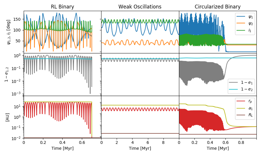
Each system has three possible general outcomes, shown in Figure 4. The final outcome depends mainly on the eccentricity excitations and the efficiency of the tides, which act to tighten and circularize the inner orbit. The “strength” of the EKL mechanism, parameterized by (Eq. 4), combined with the mutual inclination of the system determine the nature of the eccentricity excitations (Naoz 2016, e.g.,).
- •
Roche Limit (RL) crossing When extreme eccentricity excitations occur on a shorter timescale than the tidal forces can circularize the system, the pericenter approach can become smaller than the Roche-limit (Eq. 5). This type of behavior is depicted in the left hand side of Figure 4. This outcome is common in the weak-tide regime examined in this paper.
- •
Tidal tightening and circularization During periods of higher eccentricity induced by the third star, tidal forces can act to shrink and circularize the inner orbit. The tidal forces decrease the inner semi-major axis until the inner orbit decouples from the third star. The decoupling of the outer and inner orbits results in a conservation of their individual angular momenta. As a result, the typical final semi-major axis of the inner orbit is , where the subscript “0” denotes initial values. The right column of Figure 4 shows an example of this evolution.
Tidal dissipation also tends to align the spin axes of the stars with the inner orbit’s angular momentum vector. The spin-orbit angle () is defined as the angle between the inner orbit’s angular momentum and the spin axis of (). Figure 5 shows that this angle goes to zero in most systems. However, in some cases, the system can become locked into a resonance, called a Cassini resonance:
(6) where denotes the spin-orbit angle and , the spin period of the two stars () in the inner orbit (Fabrycky et al. 2007; Stephan et al. 2016; Naoz & Fabrycky 2014, e.g.,).
- •
Weak oscillations In many cases, the third star induces only weak eccentricity and inclination oscillations that do not result in a dramatic change of the orbital parameters. The middle column of Figure 4 shows an example system. While the locations of these individual systems in the eccentricity distribution shift slightly, they do not introduce a noticeable net change.

3.2 Eccentricity distribution and the effect of tides
The final eccentricity distribution tends to retain the same shape and curvature as the birth distribution irrespective of other conditions. We quantify their similarity and provide predictions in §3.4.1. This result holds for gap and no-gap simulations. To visualize this trend, we group the results by initial eccentricity distribution in Figure 6. The initial period distribution has no discernible effect on the shape of the final eccentricity distribution.
As expected, tidal efficiency results in more circularized systems, increasing the vertical axis intercept of the cumulative distribution as shown in Figure 6 for no-gap simulations. Less efficient tides result in an abundance of RL binaries, which can also increase the vertical axis intercept of the cumulative distribution. Recall that we artificially set eccentricity of the RL systems to , which may inflate the number of circularized systems. Irrespective of efficiency, tides have no effect on the overall shape or functional form (e.g., thermal) of the distribution.
3.3 Period distribution and the effect of tides
The final long period distribution tends to retain the same shape and curvature as the birth distribution irrespective of other conditions. We quantify the similarity and provide predictions in §3.4.2.
As mentioned above, we treat the RL systems as tight binaries. Figure 7 illustrates the strong dependency of the fraction of circularized systems on tidal efficiency. The dependency of RL system fraction on tidal efficiency is less pronounced, but generally less efficient tides result in more RL crossed systems. Figure 7 exemplifies this trade-off between circularized systems and RL-crossed systems, where the red curves count RL binaries. An RL crossing occurs when the EKL mechanism drives extreme eccentricity excitations before before tides can shrink and circularize the system. A lower tidal efficiency therefore gives systems more chances to cross the RL. With the exception of the blue curves in Figure 7, we include RL binaries as short-period systems unless otherwise noted.
In Figure 7, the final period distribution for gap simulations appears bimodal and exhibits a dearth of systems at intermediate periods. The peak at short-periods consists of RL and tidally tightened systems. In tidally inefficient (IET) simulations, this peak comprises RL binaries, while the vast majority of systems remain at long periods. Even with the most efficient tides (SET), Myr of EKL evolution fail to fill the gap.

Since tidal efficiency is highly sensitive to stellar radius, larger radii yield more circularized systems. Additionally, the final periods of these systems depend on the stellar radii due to angular momentum conservation (Ford & Rasio 2006). Therefore, as stars leave the main sequence and inflate, we expect circularized systems to have longer periods. To illustrate this behaviour, we consider three approaches to the mass-radius relation in Figure 8. Specifically, we consider the ZAMS mass-radius relation (blue line), as well as and the TAMS mass-radius relation, (Demircan & Kahraman 1991, e.g.,) (green and red lines, respectively). To highlight the differences, we include a gap and make the tides unrealistically efficient (UET, unrealistic equilibrium tides). As shown in the figure, the larger radii correspond to longer periods for the tidally tightened binaries. Additionally, larger radii result in a more filled gap at intermediate periods. However, even with unrealistically efficient tides, the TAMS distribution fails to match observations.

3.4 Predictions: Observable signatures of Birth Properties
3.4.1 Eccentricity
To quantify the degree of similarity between the simulated birth and final eccentricity distributions, we fit a function of the form
| (7) |
to the initial and final cumulative distributions, where is the index of the power law and and are constants. The parameters have the following limits: , , and . We argue that the vertical axis intercept, , must be greater than or equal to zero because we are fitting a cumulative distribution. We fit both the initial and final distributions to show consistency between the two. As depicted in Figure 9, changes by at most, and only for the most efficient tides. We caution that while this trend holds for hierarchical triple dynamics, we do not account for other dynamical processes that may alter the eccentricity distribution.
We vary the range of eccentricity values over which we fit. When fitting over the full range of eccentricity values, we impose the condition that to absorb all circularized and RL-crossed binary systems into the vertical-axis intercept. We also fit over the range . We recommend fitting over this range because the EKL Mechanism tends to affect high eccentricity systems the most. As these more eccentric systems circularize or cross the Roche limit, they increase the number of low eccentricity systems. Similarly, a fit of the birth distribution over this range better reflects the function used to generate values because the stability criteria target the extremes.

3.4.2 Orbital Period

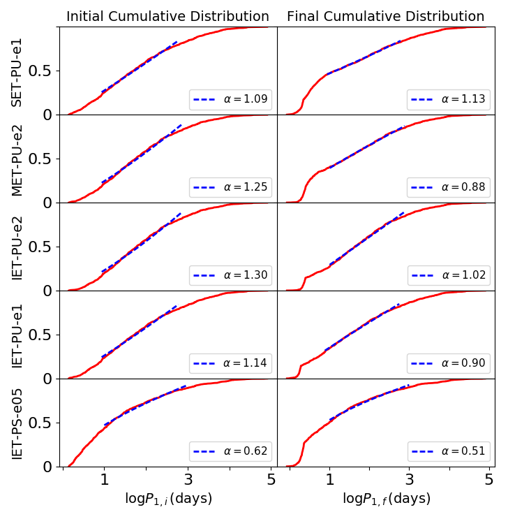
We use a function of the same form, , with the same limits on , , and . We fit the period distribution over the range . We select the lower limit to avoid the newly-formed peak of short-period systems. This lower limit must be adjusted to accommodate the width of the short-period peak, which will depend on the stellar radii (Figure 8) and therefore the age of the binary system when it circularizes. The reason for the upper limit is twofold: the stability criteria curb the number of long period systems, causing our initial distributions to converge at large period, and observational campaigns may not be sensitive to longer periods (e.g., Sana et al. 2013). The birth distribution signature proves much more difficult to discern in the period distributions than in the eccentricity distributions. We find that the orbital period distribution is most consistently preserved over this range, . The power changes by at most for PU simulations and stays for PS simulations.
3.5 Comparison to observations
3.5.1 Eccentricity Distribution
Several groups have studied the eccentricity distributions of massive binaries. Specifically, Almeida et al. 2017 have examined OB-type spectroscopic systems in the Tarantula region to find that of systems have small eccentricities (). Furthermore, their eccentricity distribution appears uniform. However, the cumulative distribution flattens slightly for high () eccentricities, indicating fewer systems there. In a study of massive systems from the Cygnus OB2 association, Kobulnicky et al. 2014 also show a flattening in the cumulative distribution at high eccentricity and attribute it to an observational bias. While this observed flattening may indeed reflect observational biases, we do find that our stability conditions curb the number of high eccentricity systems. As a result, our initial conditions exhibit flattening at large eccentricities (see Figure 1), which persists in the final distribution.
Similar to Almeida et al. 2017, Kobulnicky et al. 2014 note an abundance of low () eccentricity systems and conclude that the distribution is uniform for . In their review, Duchêne & Kraus 2013 also suggest that massive binaries follow a uniform eccentricity distribution, while Sana & Evans 2011 and Sana et al. 2012 give a probability density of the form . Moe & Di Stefano 2017 find a thermal eccentricity distribution, , for OB-type binaries using the catalog from Malkov et al. 2012. However, their finding pertains to wider binaries with periods between 10 and 100 days, and many of our systems have shorter periods.
We find that the power law index is a good indicator of the initial condition. Additionally, Geller et al. 2019 determine that star cluster dynamics has little to no effect on the shape of the eccentricity distribution for binaries with modest orbital periods. These combined results imply that the final distribution resembles the birth distribution. The birth distribution of population with uniform eccentricities is therefore also uniform.
3.5.2 Period Distribution
Duchêne & Kraus 2013 estimate that of massive binaries have periods of less than ten days. Sana & Evans 2011 find that to of systems fall at . Similarly, the data of Almeida et al. 2017 indicate an abundance () of short-period ( week) systems. Kobulnicky et al. 2014 also affirm the abundance of short-period binaries.
Counting RL binaries in the no-gap simulations, systems with represent , , and of the SET, MET, and IET inner binaries, respectively, in Figure 7. The super efficient tides (SET, first row) seem too efficient. However, counting only systems with to reflect observational limits, the SET and MET simulations match the estimates of Sana & Evans 2011 and Kobulnicky et al. 2014 with and short-period ( days) systems, respectively. The IET simulation has . Additionally, observations may not be sensitive to our so-called RL binaries. In that case, the IET tides become too inefficient to account for observations. Examining only tidally-tightened systems, the fractions of short-period binaries fall to , and of total systems with for SET, MET, and IET simulations, respectively.
A power law of the form is often fitted to the orbital period distribution (Kobulnicky et al. 2014, e.g.,). The index of this power law varies in the literature. Sana et al. 2012 suggest , while Sana et al. 2013 find . Almeida et al. 2017 conclude that an index between and reproduces the data well depending on the range over which they fit. Kobulnicky et al. 2014 suggest that tight binary peak has some structure, i.e. the distribution is not uniform at short-periods.
In Figure 11, we show the cumulative distributions for all of our no-gap simulations over the range . Bounded by the curves (Almeida et al. 2017; Kobulnicky et al. 2014) and (Sana et al. 2012; Sana et al. 2013), the gray region depicts the range of power laws fitted to observations. While several of our simulated results resemble the power laws fitted to the data, generally, SET and PS simulations seem to overpredict the number of short-period systems, while IET simulations underpredict the number of short period systems.
We perform a Kolmogorov-Smirnov (KS) two-sample test to compare our final period distributions to observations. We perform this test both with and without including RL binaries in our simulated sample. Comparing to the data of Sana et al. 2012, we cannot reject the null hypothesis that the observations and simulated results share a parent probability density distribution for the following simulations: MET-PS-e05, MET-PS-e1, SET-PU-e2, IET-PS-e05 both with and without RL binaries. We also perform this test with the data from Kobulnicky et al. 2014 and find that we cannot reject the null hypothesis for MET-PS-e05 and IET-PS-e05 without RL binaries; MET-PU-e2 and MET-PU-e05 with RL binaries; and SET-PU-e2 and SET-PU-e1 both with and without RL binaries. We do not assign much significance to these results. We have a number of systems, the RL binaries, with poorly understood periods in MET and IET no-gap simulations, which hinder a statistical comparison between our results and the data. Additionally, the data have far fewer systems and are subject to observational biases: at large periods, the observed distribution likely diverges from the intrinsic distribution (Sana et al. 2012). The latter explains why the KS test favors PS and SET simulations, while the fitted power laws more often coincide with MET-PU simulations (Figure 11).
Unlike the no-gap simulations, the gap simulations seem to be in tension with observations. We plot the cumulative distributions for the gap simulations with more efficient tides in Figure 12. The curves all exhibit a similar behavior indicative of a bimodal distribution. We again perform a KS test to compare our simulated results with the observations. The bottom panel of Figure 12 plots simulation results with the data from Sana et al. 2012 and Kobulnicky et al. 2014 that we test. We find that we can reject the null hypothesis that the simulated distributions and data are drawn from the same parent probability density distribution. Two major differences separate our simulated results from the observations: the persistence of a substantial population of long-period systems and the lack of intermediate period binaries, as illustrated by Figure 7. While the true separations of RL binaries – and whether they can fall at intermediate periods – is highly uncertain, a substantial long-period population will nonetheless persist.


4 discussion
A distant stellar companion can drive the long-term evolution of a massive stellar binary. Distant companions, which may be quite common, can therefore alter the observed orbital parameter distributions for massive binaries. We characterize these effects for a large variety of birth distributions and tidal efficiencies. We find the following:
- •
Spin-Orbit Angle Distribution: Figure 5 plots the spin-orbit angles and periods of 3000 realizations of massive triples color-coded by eccentricity. For long-period systems, no trend in spin-orbit angle and eccentricity exists. However, as systems circularize at periods of about 10 days, the orbit and stars’ angular momenta align such that the spin-orbit angle goes to zero, with a few exceptions: occasionally the spin-orbit angle becomes locked in a (non-zero) resonance, called a Cassini resonance.
- •
Eccentricity distribution: The final eccentricity distribution is an excellent indication of the birth distribution. The cumulative distribution retains the curvature of the birth distribution. Since the EKL Mechanism most affects high eccentricity systems, a fit over the range of a function quantifies this trend (see Figure 9). Generally, the change in is within , with a tendency to flatten – or render more uniform – the eccentricity distribution.
- •
Period distribution: A signature of the birth period distribution persists at . We fit the period cumulative distribution with a power law over this range. The index changes by for the uniform initial condition and remains for (PS) initial condition simulations (Figure 10).
- •
Short period binaries: Observations indicate an abundance of short-period binaries (Duchêne & Kraus 2013, e.g.,). In our simulations, the tidal efficiency determines both the resulting number of short-period binaries and the dominant type of short-period system. Less efficient tides give systems more chances to cross the Roche limit, while efficient tides yield more circularized, tight binaries. The former results in an artificial peak in our final period distribution because the final properties of such systems remain uncertain. Due to angular momentum conservation, the final period of any short-period system is proportional to the stellar radius. We treat the stellar radii as constant. However, realistically, the radii will expand as the stars age. Systems which tidally tighten or cross the Roche Limit at later times will therefore fall at longer periods (Figure 8).
- •
Initial Period Gap: Sana et al. 2017 suggest that massive binaries may form with large separations and tighten over time to match the parameter distributions of older populations. The EKL mechanism in concert with tidal dissipation represents a channel for producing hardened binaries. However, the EKL mechanism fails build up a sufficient population of short period binaries if we begin with a lower period cutoff of nine months (Figure 12).
We perform a brief calculation to assess whether type II migration may fill a 9 month gap in the inner period distribution. Following Armitage 2007, the type-II migration timescale can be written as: , where is related to the viscosity, is the scale height, and represents the disk aspect ratio. denotes the angular velocity. A nine month period corresponds to a roughly 2 AU semi-major axis. Taking the primary and secondary to have masses and , respectively, is approximately . We assume that (Ruge et al. 2013, e.g.,) and (Armitage 2007). We find that the timescale is about . Type II migration therefore represents a mechanism to bridge an initial period gap, as suggested by Sana et al. 2017, with observations of older populations. Acting over a short timescale to tighten binaries, type II migration may fill the gap in the period distribution. If a binary system undergoing migration has a third companion, the gas will mostly suppress the gravitational perturbation of the tertiary star, although the system may develop an inclination between the disk and the companion (Martin et al. 2014, e.g.,).
- •
Comparison with Observations: no initial period gap and moderate tides We compare our cumulative distributions for the final inner orbital period with the observationally constrained power laws in Figure 11. Many of our results fall in the region bounded by the power laws indicated by the literature (Almeida et al. 2017, e.g.,). Howerver, generally, simulations with moderately efficient tides (MET) and a uniform birth period distribution match observed distributions well.
Several observations indicate a uniform eccentricity distribution except at high eccentricity (Kobulnicky et al. 2014, e.g.,). Only simulations that begin with a uniform eccentricity distribution produce a uniform distribution as the end result.
Unlike previous studies of EKL evolution in triple stellar systems (Naoz & Fabrycky 2014; Bataille et al. 2018; Moe & Kratter 2018, e.g.,), we find that the final period and eccentricity distributions carry a clear signature of the initial distributions. This behavior is a consequence of the short timescale of evolution ( Myr) and the moderately efficient tides of stars with radiative envelopes. We expect that as stellar evolution increases the stellar radii and causes mass loss, the orbital configurations will significantly alter.
Acknowledgements
SN thanks Howard and Astrid Preston for their generous support. SCR acknowledges support from the Eugene Cota-Robles Fellowship.
References
- Almeida et al. (2017) Almeida L. A., et al., 2017, A&A, 598, A84
- Antonini & Perets (2012) Antonini F., Perets H. B., 2012, ApJ, 757, 27
- Armitage (2007) Armitage P. J., 2007, preprint, pp astro–ph/0701485 (arXiv:astro-ph/0701485)
- Bataille et al. (2018) Bataille M., Libert A.-S., Correia A. C. M., 2018, MNRAS, 479, 4749
- Bouvier (2013) Bouvier J., 2013, in Hennebelle P., Charbonnel C., eds, EAS Publications Series Vol. 62, EAS Publications Series. pp 143–168 (arXiv:1307.2891), doi:10.1051/eas/1362005
- Chernov (2017) Chernov S. V., 2017, Astronomy Letters, 43, 429
- Claret & Cunha (1997) Claret A., Cunha N. C. S., 1997, A&A, 318, 187
- Demircan & Kahraman (1991) Demircan O., Kahraman G., 1991, Ap&SS, 181, 313
- Duchêne & Kraus (2013) Duchêne G., Kraus A., 2013, ARA&A, 51, 269
- Eggleton (1983) Eggleton P. P., 1983, ApJ, 268, 368
- Eggleton & Kiseleva-Eggleton (2001) Eggleton P. P., Kiseleva-Eggleton L., 2001, ApJ, 562, 1012
- Eggleton et al. (1998) Eggleton P. P., Kiseleva L. G., Hut P., 1998, ApJ, 499, 853
- Eggleton et al. (2007) Eggleton P. P., Kisseleva-Eggleton L., Dearborn X., 2007, in Hartkopf W. I., Harmanec P., Guinan E. F., eds, IAU Symposium Vol. 240, Binary Stars as Critical Tools: Tests in Contemporary Astrophysics. pp 347–355, doi:10.1017/S1743921307004280
- Fabrycky & Tremaine (2007) Fabrycky D., Tremaine S., 2007, ApJ, 669, 1298
- Fabrycky et al. (2007) Fabrycky D. C., Johnson E. T., Goodman J., 2007, ApJ, 665, 754
- Ford & Rasio (2006) Ford E. B., Rasio F. A., 2006, ApJ, 638, L45
- Geller et al. (2019) Geller A. M., Leigh N. W. C., Giersz M., Kremer K., Rasio F. A., 2019, ApJ, 872, 165
- Grellmann et al. (2013) Grellmann R., Preibisch T., Ratzka T., Kraus S., Helminiak K. G., Zinnecker H., 2013, A&A, 550, A82
- Griffin (2012) Griffin R. F., 2012, Journal of Astrophysics and Astronomy, 33, 29
- Harrington (1969) Harrington R. S., 1969, Celestial Mechanics, 1, 200
- Hoang et al. (2018) Hoang B.-M., Naoz S., Kocsis B., Rasio F. A., Dosopoulou F., 2018, ApJ, 856, 140
- Hurley et al. (2002) Hurley J. R., Tout C. A., Pols O. R., 2002, MNRAS, 329, 897
- Katz & Dong (2012) Katz B., Dong S., 2012, arXiv e-prints, p. arXiv:1211.4584
- Kiseleva et al. (1998) Kiseleva L. G., Eggleton P. P., Mikkola S., 1998, MNRAS, 300, 292
- Kobulnicky et al. (2014) Kobulnicky H. A., et al., 2014, ApJS, 213, 34
- Kozai (1962) Kozai Y., 1962, AJ, 67, 591
- Langer (2009) Langer N., 2009, A&A, 500, 133
- Lidov (1962) Lidov M. L., 1962, planss, 9, 719
- Malkov et al. (2012) Malkov O. Y., Tamazian V. S., Docobo J. A., Chulkov D. A., 2012, A&A, 546, A69
- Mardling & Aarseth (2001) Mardling R. A., Aarseth S. J., 2001, MNRAS, 321, 398
- Martin et al. (2014) Martin R. G., Nixon C., Lubow S. H., Armitage P. J., Price D. J., Doğan S., King A., 2014, ApJ, 792, L33
- Mazeh & Shaham (1979) Mazeh T., Shaham J., 1979, A&A, 77, 145
- Michaely & Perets (2014) Michaely E., Perets H. B., 2014, ApJ, 794, 122
- Moe & Di Stefano (2017) Moe M., Di Stefano R., 2017, ApJS, 230, 15
- Moe & Kratter (2018) Moe M., Kratter K. M., 2018, ApJ, 854, 44
- Mylläri et al. (2018) Mylläri A., Valtonen M., Pasechnik A., Mikkola S., 2018, MNRAS, 476, 830
- Naoz (2016) Naoz S., 2016, ARA&A, 54, 441
- Naoz & Fabrycky (2014) Naoz S., Fabrycky D. C., 2014, preprint, (arXiv:1405.5223)
- Naoz et al. (2013a) Naoz S., Farr W. M., Lithwick Y., Rasio F. A., Teyssandier J., 2013a, MNRAS, 431, 2155
- Naoz et al. (2013b) Naoz S., Kocsis B., Loeb A., Yunes N., 2013b, ApJ, 773, 187
- Naoz et al. (2016) Naoz S., Fragos T., Geller A., Stephan A. P., Rasio F. A., 2016, ApJ, 822, L24
- Pejcha et al. (2013) Pejcha O., Antognini J. M., Shappee B. J., Thompson T. A., 2013, MNRAS, 435, 943
- Perets & Fabrycky (2009) Perets H. B., Fabrycky D. C., 2009, ApJ, 697, 1048
- Preibisch et al. (2001) Preibisch T., Weigelt G., Zinnecker H., 2001, in Zinnecker H., Mathieu R., eds, IAU Symposium Vol. 200, The Formation of Binary Stars. p. 69 (arXiv:astro-ph/0008014)
- Pribulla & Rucinski (2006) Pribulla T., Rucinski S. M., 2006, AJ, 131, 2986
- Prodan et al. (2015) Prodan S., Antonini F., Perets H. B., 2015, ApJ, 799, 118
- Raghavan et al. (2010) Raghavan D., et al., 2010, ApJS, 190, 1
- Ruge et al. (2013) Ruge J. P., Wolf S., Uribe A. L., Klahr H. H., 2013, A&A, 549, A97
- Sana & Evans (2011) Sana H., Evans C. J., 2011, in Neiner C., Wade G., Meynet G., Peters G., eds, IAU Symposium Vol. 272, Active OB Stars: Structure, Evolution, Mass Loss, and Critical Limits. pp 474–485 (arXiv:1009.4197), doi:10.1017/S1743921311011124
- Sana et al. (2012) Sana H., et al., 2012, Science, 337, 444
- Sana et al. (2013) Sana H., et al., 2013, A&A, 550, A107
- Sana et al. (2017) Sana H., Ramírez-Tannus M. C., de Koter A., Kaper L., Tramper F., Bik A., 2017, A&A, 599, L9
- Shappee & Thompson (2013) Shappee B. J., Thompson T. A., 2013, ApJ, 766, 64
- Stephan et al. (2016) Stephan A. P., Naoz S., Ghez A. M., Witzel G., Sitarski B. N., Do T., Kocsis B., 2016, preprint, (arXiv:1603.02709)
- Thompson (2011) Thompson T. A., 2011, ApJ, 741, 82
- Tokovinin (1997) Tokovinin A. A., 1997, Astronomy Letters, 23, 727
- Tokovinin (2008) Tokovinin A., 2008, MNRAS, 389, 925
- Toonen et al. (2018) Toonen S., Perets H. B., Igoshev A. P., Michaely E., Zenati Y., 2018, A&A, 619, A53
- Yoon et al. (2010) Yoon S.-C., Woosley S. E., Langer N., 2010, ApJ, 725, 940
- Zahn (1977) Zahn J.-P., 1977, A&A, 57, 383
- Zinnecker & Yorke (2007) Zinnecker H., Yorke H. W., 2007, ARA&A, 45, 481
Appendix A Simulation Parameters
We run several large Mont-Carlo simulations to cover a wide range of initial conditions. Table 2 describes the 38 sets of Monte-Carlo simulations. Some simulations adopt a Kroupa mass function with limits (“K1”) or (“K6”). We find that the masses affect the results insofar as they determine the tidal efficiency. For example, for the former limits, the abundance of low mass stars with efficient tides will result in more circularized systems even when using the IET prescription.
| Label | Radius | Mass | Eccentricity | Period | Tides |
| PU-e1-M10-TAMS | TAMS | & Uniform | Uniform | Uniform | SET |
| PU-e1-M10-Emp | Empirical | & Uniform | Uniform | Uniform | SET |
| PU-e1-M10-ZAMS | ZAMS | & Uniform | Uniform | Uniform | SET, MET, IET, UET(g), SET(g), MET(g), IET(g) |
| PS-e1-M10-ZAMS | ZAMS | & Uniform | Uniform | SET, MET, SET(g) | |
| PS-e05-M10-TAMS | TAMS | & Uniform | UET(g) | ||
| PS-e05-M10-Emp | Empirical | & Uniform | UET(g), LET(g) | ||
| PS-e05-M10-ZAMS | ZAMS | & Uniform | MET, IET, UET(g), SET(g), MET(g) | ||
| PU-e05-M10-ZAMS | ZAMS | & Uniform | MET | ||
| PU-e2-M10-ZAMS | ZAMS | & Uniform | Thermal | Uniform | SET, MET, IET, SET(g), MET(g) |
| PS-e2-K6-Emp | Empirical | Kroupa with | Thermal | LET(g) | |
| PS-e05-K6-Emp | Empirical | Kroupa with | LET(g) | ||
| PU-e05-K6-Emp | Empirical | Kroupa with | Uniform | LET(g) | |
| PU-e2-K6-Emp | Empirical | Kroupa with | Thermal | Uniform | LET(g) |
| PS-e1-K1-ZAMS | ZAMS | Kroupa with | Uniform | IET(g) | |
| PU-e1-K1-ZAMS | ZAMS | Kroupa with | Uniform | IET | |
| PU-e1-K6-ZAMS | ZAMS | Kroupa with | Uniform | LET | |
| PU-e2-K1-ZAMS | ZAMS | Kroupa with | Thermal | Uniform | IET(g) |
| PS-e05-K1-ZAMS | ZAMS | Kroupa with | IET(g) | ||
| PS-e2-K1-ZAMS | ZAMS | Kroupa with | Thermal | IET | |
| PU-e05-K1-ZAMS | ZAMS | Kroupa with | Uniform | IET | |
| PU-e05-K6-ZAMS | ZAMS | Kroupa with | Uniform | LET |
Appendix B Fitting the Period Distribution
Taking a similar approach to Section 3.4.2, we fit the cumulative no-gap period distribution over the range , selected to reflect the limits in, for example, Almeida et al. 2017 and Sana et al. 2013, in figure 13. With , PU-MET simulations best match observationally constrained cumulative distribution functions which have . We show additional examples in 14. The IET-PU distributions are too flat, while either SET or PS conditions give too pronounced curvature with . Taking the observations and our fits at face value, we suggest that moderately efficient tides – or another model with a similar efficiency – are the best candidate. However, these fits remain uncertain because of the RL binaries, included in the cumulative distribution.
We further suggest that cumulative distributions be fitted in two parts: one where the short-period peak occurs and one for periods longer that days. Since MET-PU simulations yield a similar final period distribution irrespective of eccentricity initial condition, we fit the MET-PU-e1 results as an example in Figure 15.


Appendix C Additional Examples of Period Distribution Traces
We apply the method described in Section 3.4.2 to all of our no-gap simulations to find traces of the initial period distribution in the final result. We show the other five simulations here. As noted in Section 3.4.2, the index of the power law fitted over the range changes by at most for PU simulations and stays for PS simulations.