Time series models for realized covariance matrices based on the matrix-F distribution
We propose a new Conditional BEKK matrix-F (CBF) model for the time-varying realized covariance (RCOV) matrices. This CBF model is capable of capturing heavy-tailed RCOV, which is an important stylized fact but could not be handled adequately by the Wishart-based models. To further mimic the long memory feature of the RCOV, a special CBF model with the conditional heterogeneous autoregressive (HAR) structure is introduced. Moreover, we give a systematical study on the probabilistic properties and statistical inferences of the CBF model, including exploring its stationarity, establishing the asymptotics of its maximum likelihood estimator, and giving some new inner-product-based tests for its model checking. In order to handle a large dimensional RCOV matrix, we construct two reduced CBF models — the variance-target CBF model (for moderate but fixed dimensional RCOV matrix) and the factor CBF model (for high dimensional RCOV matrix). For both reduced models, the asymptotic theory of the estimated parameters is derived. The importance of our entire methodology is illustrated by simulation results and two real examples.
, , and
University of Florida??, Tsinghua University,??
The University of Hong Kong?? and The Education University of Hong Kong??
1 Introduction
Modeling the multivariate volatility of many asset returns is crucial for asset pricing, portfolio selection, and risk management. After the seminal work of Barndorff-Nielsen and Shephard (2002, 2004) and Andersen et al. (2003), the realized covariance (RCOV) matrix, estimated from the intra-day high frequency return data, has been recognized as a better estimator than the daily squared returns for daily volatility. Consequently, increasing attention has been focused on the modeling and forecasting of these RCOVs; see, e.g., McAleer and Medeiros (2008), Hansen et al. (2012), Noureldin et al. (2012), Bollerslev et al. (2016), and many others.
Existing models for the RCOV matrices can be roughly categorized into two types: transformation-based models and likelihood-based models. Models in the first category capture the dynamics of the RCOV matrices in an indirect way via transformation. Bauer and Vorkink (2011) used a factor model for the vectorization of the log transformation of RCOV matrix; Chiriac and Voev (2011) applied a vector autoregressive fractionally integrated moving average process to model the Cholesky decomposition of RCOV matrix; Callot et al. (2017) transformed the RCOV matrix into a large vector by the operator, and then fitted this transformed vector by a vector autoregressive model. In the first two models, the dimension of RCOV matrix has to be moderate (e.g., less than 6) for a feasible manipulation. In the third model, the dimension of RCOV matrix is allowed to be 30 in applications with the help of the LASSO method.
Models in the second category deals with RCOV matrices directly by assuming that the innovation, which drives the RCOV time series, has a specific matrix distribution to generate random positive definite matrices automatically without imposing additional constraints. This important feature results in positive-definite estimated RCOV matrices. Unlike scalar or vector distributions, so far only few matrix distributions have been found to have explicit forms. The primary choice for the innovation distribution is Wishart, leading to the Wishart autoregressive (WAR) model in Gouriéroux et al. (2009), the conditional autoregressive Wishart (CAW) model in Golosnoy et al. (2012), the mixture Wishart model in Jin and Maheu (2013, 2016), and the generalized CAW model in Yu et al. (2017) to name a few. The other choice for the innovation distribution is matrix-F, which was recently adopted by Opschoor et al. (2018). Generally speaking, matrix-F distribution is the generalization of the usual F distribution, while Wishart distribution is the generalization of the distribution (see, e.g., Konno (1991) and Opschoor et al. (2018) for more discussions). Therefore, matrix-F distribution could be more appropriate than Wishart distribution in capturing the heavy-tailed innovation, which is an important stylized fact in many applications (see, e.g., Bollerslev (1987), Fan et al. (2014), Zhu and Li (2015), and Oh and Patton (2017)). These likelihood models have at least three edges over the transformation-based models. First, the likelihood-based models will preserve the useful and important matrix structural information, which makes them more interpretable compared with transformation-based models. Second, the number of estimated parameters in the transformation-based models has order , while the one in the likelihood-based models has order , where is the dimension of the RCOV matrix. When is large, the likelihood-based models can bring more convenience and a less daunting task in computation. Third, the likelihood-based models make use of the likelihood function of the RCOV matrices, and hence their statistical inference methods could be easily provided.
This paper contributes to the literature from three aspects. First, we propose a new Conditional BEKK matrix-F (CBF) model to study the time-varying RCOV matrices. Our CBF model has matrix-F distributed innovations with two degrees of freedom parameters and . When , our CBF model reduces to the CAW model (Golosnoy et al., 2012), which has Wishart distributed innovations. Hence, the degrees of freedom is designed to capture the heavy-tailedness of the RCOV. Since the RCOV is also well documented to have long memory phenomenon, we further introduce a special CBF model which has a similar conditional heterogeneous autoregressive (HAR) structure as in Corsi (2009). This special model is coined the CBF-HAR model. Although the CBF-HAR model is not formally a long memory model, it gives rise to persistence in the RCOV time series. Two real examples demonstrate that our CBF model (especially the CBF-HAR model) can have a significantly better forecasting performance than the corresponding CAW model, and hence a simple incorporation of to capture the heavy-tailed RCOV is necessary from a practical viewpoint.
Second, we provide a systematically statistical inference procedure for the CBF model. Specifically, we explore its stationarity conditions, establish the strong consistency and asymptotic normality of its maximum likelihood estimator (MLE), and investigate some new inner-product-based tests for model diagnostic checking. Moreover, the performance of our entire methodology is assessed by simulation studies. Compared to the existing BEKK-type multivariate time series models, our proofs of the entire inference procedure are much involved, since the CBF model is tailored for matrix time series. Particularly, our inner-product-based tests seem to be the first diagnostic checking tool for matrix time series models, and the related idea can be easily extended to other models.
Third, we construct two reduced CBF models — the variance targeted (VT) CBF (VT-CBF) model and the factor CBF (F-CBF) model, to handle moderately large and high dimensional RCOV matrix respectively. For both reduced models, the asymptotic theory of the estimated parameters is derived. The dimension of the RCOV matrix is allowed to be a moderate but fixed number in the VT-CBF model, while it is allowed to grow with the sample size and the intra-day sample size in the F-CBF model. Therefore, this makes the prediction of large dimensional RCOV matrices feasible in many cases. The importance of both reduced models is illustrated by two real applications.
The remainder of this paper is organized as follows. Section 2 introduces the CBF model and studies its probabilistic properties. Section 3 investigates the asymptotics of the MLE. Section 4 presents inner-product-based tests to check the model adequacy. Two reduced CBF models and their related asymptotic theories are provided in Section 5. Some simulation studies are carried out in Section 6. Applications are given in Section 7. Section 8 concludes this paper. Proofs of all theorems are relegated to the supplementary material.
Some notations are used throughout the paper. is the identity matrix of order , and represents the Kronecker product. For an matrix , is its trace, is its transpose, is its determinant, is its biggest eigenvalue, is its Euclidean (or Frobenius) norm, is its spectral norm, is a vector obtained by stacking all the columns of , is a vector obtained by stacking all columns of the lower triagular part of , and .
2 Model and Properties
2.1 Model specification
Let be the integrated volatility matrix of asset returns at time . After the seminal work of Barndorff-Nielsen and Shephard (2002, 2004) and Andersen et al. (2003), the positive definite realized covariance (RCOV) matrix calculated from the high-frequency return data of has been widely applied to estimate in the literature; see, e.g., Barndorff-Nielsen et al. (2011), Lunde et al. (2016), Aït-Sahalia and Xiu (2017), Kim et al. (2018) and references therein. Moreover, is often viewed as a precise estimate for the conditional variances and covariances of these low-frequency asset returns , and hence how to predict by some dynamic models is important in practice. Motivated by this, a new dynamic model for is proposed in the current paper.
Let be a filtration up to time . We assume that
| (2.1) |
where is a sequence of independent and identically distributed (i.i.d.) positive definite random innovation matrices with , each follows the matrix-F distribution , and the density of is
| (2.2) |
where with degrees of freedom and , is an positive definite matrix, and
moreover, is the square root of the positive definite matrix , which has a BEKK-type dynamic structure (see Engle and Kroner, 1995):
| (2.3) |
where , , are all real matrices, the integers are known as the orders of the model, and as well as the initial states are all positive definite. Under model (2.1),
| (2.4) |
with , that is, the conditional distribution of is matrix-F with a BEKK-type mean structure. In this sense, we call model (2.1) the Conditional BEKK matrix-F (CBF) model.
The CBF model is related to the CAW model in Golosnoy et al. (2012), in which follows the Wishart distribution. To see it clearly, we follow Konno (1991) and Leung and Lo (1996) to re-write in model (2.1) as
| (2.5) |
where and are independent. As in probability, the identity (2.5) implies that when , , which is exactly the CAW model. Therefore, compared to the CAW model, the degrees of freedom in the CBF model accommodates the heavy-tailed RCOV, meaning that each from satisfying (2.4) could have a heavier tail than that from satisfying (see, e.g., Opschoor et al. (2018) for more discussions and examples). Clearly, the identity (2.5) also guarantees to be symmetric and positive definite, and it can be used to generate by using Wishart random variables.
Besides the heavy-tailedness, long memory is another well documented feature for the RCOV, and it has been taken into account by many RCOV models, including the heterogeneous autoregressive (HAR) model in Corsi (2009) as a benchmark. Although the HAR model does not formally belong to the class of long memory models, it is able to reproduce the persistence of RCOV observed in many empirical data. Inspired by the HAR model, we consider a special CBF model, which has the following specification for :
| (2.6) |
where , , and are the daily, weekly, and monthly averages of RCOV matrices, respectively. In this case, we label model (2.1) as the CBF-HAR model, since we put “HAR dynamics” on . Clearly, the CBF-HAR model is simply a constrained CBF model with , and . Figure 1 plots the sample autocorrelation functions (ACFs) up to lag 100 of one simulated data from the CBF-HAR model with and
From this figure, we can find that all entries of exhibit long memory phenomenon as expected.

Note that when , sufficient identifiability conditions of model (2.3) are that the main diagonal elements of and the first diagonal element of each , are positive; when , some sufficient identifiability conditions of model (2.3) can be found in Engle and Kroner (1995). For simplicity, we assume subsequently that model (2.3) is identifiable.
Of course, the BEKK specification in model (2.3) is not the only way to describe the dynamics of . The multivariate ARCH-type models such as the VEC model in Bollerslev et al. (1988), the component model in Engle and Lee (1999), the dynamic conditional correlation model in Engle (2002) and many others can also be adopted to model . Using these models together with the matrix-F distribution to fit and predict the RCOV matrices could be a promising direction for future study.
2.2 Stationarity
Stationarity is an important issue for most RCOV models, but so far it has been rarely studied. Denote . For , let
where for and for . A sufficient condition for the stationarity of the CBF model is given below, and it works for other general distributions of .
Theorem 2.1.
Suppose that in model (2.1) is a sequence of i.i.d. positive definite random matrices with , and
(H1) the distribution of , denoted by , is absolute continuous with respect to the Lebesgue measure;
(H2) the point is in the interior of the support of ;
(H3) .
Then, in model (2.1) is strict stationary with . Moreover, is positive Harris recurrent and geometrically ergodic.
Remark 1.
The results of Theorem 2.1 are similar to those in Boussama et al. (2011), where the stationarity of the BEKK model is studied. Like Boussama et al. (2011), the proof of Theorem 2.1 is based on the semi-polynomial Markov chains technique, however, it is much involved due to the matrix nature of model (2.1).
As a special case, the results in Theorem 2.1 hold for the CAW model, in which follows the Wishart distribution. Under conditions (H1) and (H2), condition (H3) is necessary and sufficient for the strict stationarity of with . However, the necessary and sufficient condition for the higher moments of is still unclear at this stage. Let be the permutation matrix such that for any matrix . If , it is not hard to see
(i) ;
(ii) ,
where with
and , for . Result (ii) above clearly indicates that the parameters and have impact on the second moment of in a non-linear way. Although a closed form of third moment of is absent, similar impact from and is expected for the third moment of and hence the asymptotic distribution of the proposed estimator (see Theorem 3.2 below).
3 Maximum Likelihood Estimation
Let be the unknown parameter of model (2.1) with the true value , where is the parametric space with and , , , , and . Below, we assume that and are compact and is an interior point of .
Given the observations and the initial values , the negative log-likelihood function based on (2.4) is
| (3.1) |
where
with and calculated recursively by
| (3.2) |
Clearly, .
As the initial values are not observable, we shall modify as
| (3.3) |
where is defined in the same way as with being replaced by , and is calculated in the same way as based on a sequence of given constant matrices . The minimizer, , of on is called the maximum likelihood estimator (MLE) of . That is,
| (3.4) |
To study the asymptotic properties of , we need two assumptions below.
Assumption 3.1.
is strictly stationary and ergodic.
Assumption 3.2.
For , if , almost surely (a.s.) for all .
Assumption 3.1 is standard, and Assumption 3.2 which is in line with Comte and Lieberman (2003) and Hafner and Preminger (2009) is the identification condition. The following two theorems give the consistency and asymptotic normality of , respectively.
Based on the observations and a sequence of given constant matrices , we can use the analytic expression of (see Appendix D in the supplementary material) to estimate by its sample counterpart. As the univariate ARCH-type models, the coefficients in the main diagonal line of are positive to ensure the positive definite of . Hence, the classical or Wald test, which is constructed by the estimate of , can not be used to detect whether their values are zeros; see Li et al. (2018) for more discussions on this context.
4 Model Diagnostic Checking
Diagnostic tests are crucial for model checking in multivariate time series analysis; see, e.g., Li and McLeod (1981), Ling and Li (1997), Tse (2002) and many others. However, no attempt has been made for the stationary matrix time series. In this section, we propose some new inner-product-based tests to check the adequacy of model (2.1).
Let be the vectorized residual for a given , and be the inner product of two vectorized residuals at lag . Then, we stack up to lag to construct , where
and is a given integer. Our testing idea is motivated by the fact that if model (2.1) is adequate, is a sequence of i.i.d. random vectors with mean zero, and hence the value of is expected to be close to zero. To implement our test, we need study the asymptotic property of in the following theorem.
Theorem 4.1.
Based on Theorem 4.1, we construct the inner-product-based test statistic
| (4.1) |
to detect the adequacy of model (2.1), where is the sample counterpart of . If is larger than the upper-tailed critical value of , the fitted model (2.1) is not adequate at a given significance level. Otherwise, it could be deemed as adequate.
Note that if we consider a test based on directly, the resulting limiting distribution shall still be chi-squared, but its degrees of freedom increases fast with the dimension . To avoid this dilemma, we use the inner product of the residuals to construct our test , whose limiting distribution is independent of . This new idea is different from the portmanteau test in Ling and Li (1997) in which the test statistic is constructed based on the auto-correlations of the transformed scale residuals, while our test is based on the auto-covariances of the original vectorized residuals. Clearly, our idea can be easily extended to the framework in Ling and Li (1997). Meanwhile, our inner-product-based test takes the auto-covariances of all entries of into account, while the idea of regression-based test in Tse (2002) only considers one entry of at a time. In view of this, we prefer to use the proposed inner-product idea for testing purpose.
5 The Reduced CBF Models
As the number of parameters in the CBF model is , the estimation of the CBF model could be very computationally demanding when is large. This section introduces two reduced CBF models, which are feasible in fitting RCOV matrices with a large .
5.1 The VT-CBF model
This subsection proposes a reduced CBF model by using the variance target (VT) technique in Engle and Mezrich (1996). The idea of VT is to re-parameterize the drift matrix by using the theoretical mean of , so that the estimation of is excluded in the implementation of the maximum likelihood estimation. Other related studies on the VT time series models can be found in Francq et al. (2011) and Pedersen and Rahbek (2014).
To define our reduced model, we assume that is strictly stationary with a finite mean . By taking expectation on both sides of (2.3), we have
| (5.1) |
due to the fact that . With the help of (5.1), model (2.1) becomes
| (5.2) |
where all notations are inherited from model (2.1), except that
| (5.3) |
We call model (5.2) the VT-CBF model. Clearly, this reduced model shares the same probabilistic properties as the full CBF model. Although the VT-CBF model has the same amount of parameters as the full CBF model, its two-step estimator given below is computationally easier than the MLE for the full CBF model.
To present this two-step estimator, we let be the unknown parameters of model (5.2) and its true value be , where is the parametric space with , and . Let with , and . As before, we assume that and are compact and is an interior point of .
In the first step, we estimate by , where . In the second step, we estimate the remaining parameters by the constrained MLE based on the following modified log-likelihood function:
| (5.4) |
where
and is calculated recursively by
| (5.5) |
based on a sequence of given constant matrices . Clearly, is analogous to in (3.3), and it is the modification of the following log-likelihood function:
| (5.6) |
where is defined in the same way as with being replaced by , and is calculated recursively by
| (5.7) |
based on the observations and the initial values . The minimizer, , of on is the constrained MLE of . That is,
| (5.8) |
Now, we call the two-step estimator of in model (5.2). Let and . The following two theorems give the consistency and asymptotic normality of , respectively.
As before, we can use the sample counterpart of the analytic expressions of and to estimate . Although the VT-CBF model can be estimated by the aforementioned two-step estimation procedure, it still has to handle a large number of estimated parameters with order caused by the parameter matrices and . To make a more parsimonious VT-CBF model, we can further impose some restrictions on and . McCurdy and Stengos (1992) and Engle and Kroner (1995) have suggested to use diagonal volatility models, which not only avoid over-parameterization, but also reflect the fact that the variances and the covariances rely more on its own past than the history of other variances or covariances. Motivated by this, we can assume that all and have a diagonal structure, leading to a diagonal VT-CBF model. Clearly, the number of estimated parameters in the diagonal VT-CBF model has order , which is feasible to be handled for a moderate large but fixed .
Next, similar to in (4.1), we can construct the inner-product-based test statistics to check the adequacy of model (2.1) based on the two-step estimator . Let , , be the residual vector for a given , be the inner product of the residuals at lag , and
The asymptotic property of is given in the following theorem.
Theorem 5.3.
5.2 The factor CBF model
In modern data analysis, the dimension could be growing with the sample size in many cases, and this makes the CBF (or VT-CBF) models computationally infeasible. Also, the dimension may be proportional to (the average intra-day sample size across all assets and all days), and then the methods to calculate used for the fixed deliver an inconsistent estimator of ; see, e.g., Wang and Zou (2010) and Tao et al. (2011) for surveys. To overcome this difficulty, we use the thresholding average realized volatility matrix (TARVM) estimator in Tao et al. (2011) to calculate . The TARVM is built based on the ARVM (Wang and Zou, 2010), which is constructed by taking the average of the constructed realized volatility matrices according to different predetermined sampling frequencies. The TARVM further thresholds the elements in each estimated RCOV matrix from the ARVM method, so that certain sparsity structure is retained and the resulting estimator is consistent for large , which can be growing with (or even larger than) . For more recent works in this direction, we refer to Aït-Sahalia and Xiu (2017), Kim et al. (2018), and the references therein.
Since the dimension of could be very large, it seems hard to study the dynamics of without imposing some specific structure. Here, we adopt the factor model proposed by Tao et al. (2011) by assuming that
| (5.11) |
where is an positive definite factor covariance matrix with being a fixed integer (much smaller than ), is an positive definite constant matrix, and is an factor loading matrix normalized by the constraint . In model (5.11), the dynamic structure of is driven by that of a lower-dimensional latent process , while represents the static part of .
In (5.11), we shall highlight that only the column space of can be identified, and is not identified even if is imposed. This is because is unchanged when and are replaced by and , respectively, where is any matrix satisfying .
Define
and
Then, we estimate , and by
| (5.12) |
respectively, where are the eigenvectors of corresponding to its largest eigenvalues. As suggested by Lam and Yao (2012) and Ahn and Horenstein (2013), we may select such that the largest ratios of adjacent eigenvalues are significantly larger.
In order to study the asymptotics of the proposed estimators, we introduce the following technical assumptions.
Assumption 5.1.
All row vectors of and satisfy the sparsity condition below. For an -dimensional vector , we say it is sparse if it satisfies
where , is a positive constant, and is a deterministic function of that grows slowly in with typical examples or .
Assumption 5.2.
The factor model (5.11) has fixed factors, and matrices and satisfy and for , where is the -th diagonal entry of , and .
Assumption 5.3.
for some rate function such that .
Assumptions 5.1-5.3 are sufficient to prove the consistency of . For TARVM, we can take and with so that for large ; see Tao et al. (2011). Note that Assumptions 5.1-5.3 do not rule out the case that is larger than , as long as grows more slowly than . For other estimators, the rate may be improved; see Tao et al. (2013) for more discussions.
Theorem 5.4.
(i) ,
(ii) ,
where , and with being the eigenvectors of corresponding to its largest eigenvalues.
The above theorem indicates that is a consistent estimator of rather than . Next, we assume that satisfies the CBF model, that is,
| (5.13) |
with , where is defined in the same way as in (2.3) with replaced by , and the remaining notations and set-ups inherent from model (2.1). We call models (5.11) and (5.13) the factor CBF (F-CBF) model. Particularly, if has the HAR dynamical structure as in (2.6), the resulting model is called the factor CBF-HAR (F-CBF-HAR) model. Based on this model, we have . Since , it implies that we can study the large dimensional matrix by using an low-dimensional matrix .
As is not observable, we should estimate model (5.13) based on , and hence we consider a feasible MLE of in model (5.13) given by
where is defined in the same way as in (3.3) with and replaced by and , respectively. The following theorem shows that is consistent with the ideal MLE based on , where
and is defined in the same way as in (3.1) with and replaced by and , respectively.
Theorem 5.5.
Suppose that the conditions in Theorem 5.4 hold. Then, as go to infinity, .
Since the dimension of is (much smaller than ), the calculation of is computationally feasible. In order to further reduce the number of parameters in model (5.13), we can also assume that follows a VT-CBF model. This leads to the F-VT-CBF model, which includes the F-VT-CBF-HAR model as a special case. For this F-VT-CBF model, we consider its feasible two-step estimator , where
and is defined in the same way as in (5.4) with and replaced by and , respectively. Similar to Theorem 5.5, is consistent with the ideal two-step estimator based on , where
and is defined in the same way as in (5.6) with and replaced by and , respectively.
6 Simulation
In this section, we first assess the performance of the MLE and the two-step estimator in the finite sample. We generate 1000 replications of sample size and from the following model:
| (6.1) |
where
is a sequence of independent distributed random matrices with , and or . For each repetition, we calculate , , and their related asymptotic standard deviations. For , we report the results related to instead of , and hence the asymptotic standard deviation of the estimated parameters in is absent in this case.
Table 1 reports the sample bias, the sample standard deviation (SD) and the average asymptotic standard deviation (AD) of and . From this table, we can see that the biases of both estimators are small comparing to the magnitude of the parameters, and they become smaller as the sample size increases. This assures the accuracy of both estimators. Furthermore, we find that the SDs are generally close to the ADs for both estimators, and all of the SDs and ADs become smaller as increases from 1000 to 2000. In terms of ADs or SDs, is generally more efficient than , although this efficiency advantage is weak for many parameters. However, the estimation time for is almost 70% of the time for , and this computation advantage can be more significant when increases.
| T | |||||||||||||||||
|---|---|---|---|---|---|---|---|---|---|---|---|---|---|---|---|---|---|
| Case 1 | 1000 | Bias | 0.0320 | 0.0160 | -0.0014 | -0.0029 | -0.0009 | -0.0151 | -0.0112 | -0.0102 | -0.0005 | 0.0028 | 0.0057 | -0.0009 | 0.0037 | 0.0053 | |
| ESD | 0.3914 | 0.2452 | 0.0255 | 0.0249 | 0.0240 | 0.1170 | 0.0964 | 0.0728 | 0.0600 | 0.0188 | 0.0337 | 0.0419 | 0.0248 | 0.0601 | |||
| ASD | 0.4111 | 0.2563 | 0.0258 | 0.0259 | 0.0241 | 0.1103 | 0.0892 | 0.0652 | 0.0586 | 0.0179 | 0.0323 | 0.0402 | 0.0232 | 0.0562 | |||
| Bias | -0.0080 | 0.0382 | -0.0005 | -0.0030 | 0.0000 | -0.0130 | -0.0088 | -0.0096 | -0.0020 | 0.0020 | 0.0047 | -0.0030 | 0.0033 | 0.0040 | |||
| ESD | 0.3884 | 0.2607 | 0.0263 | 0.0272 | 0.0255 | 0.1165 | 0.0956 | 0.0728 | 0.0614 | 0.0229 | 0.0366 | 0.0433 | 0.0291 | 0.0615 | |||
| ASD | 0.4024 | 0.2619 | 0.0266 | 0.0282 | 0.0258 | 0.1207 | 0.1046 | 0.0742 | |||||||||
| 2000 | Bias | 0.0188 | 0.0072 | -0.0003 | -0.0018 | -0.0002 | -0.0111 | -0.0036 | -0.0034 | 0.0019 | 0.0014 | 0.0030 | -0.0008 | 0.0012 | 0.0014 | ||
| ESD | 0.2767 | 0.1733 | 0.0174 | 0.0179 | 0.0168 | 0.0797 | 0.0633 | 0.0459 | 0.0431 | 0.0130 | 0.0231 | 0.0293 | 0.0169 | 0.0405 | |||
| ASD | 0.2880 | 0.1797 | 0.0181 | 0.0182 | 0.0169 | 0.0767 | 0.0615 | 0.0447 | 0.0417 | 0.0124 | 0.0226 | 0.0287 | 0.0162 | 0.0395 | |||
| Bias | -0.0020 | 0.0196 | 0.0002 | -0.0020 | 0.0003 | -0.0103 | -0.0024 | -0.0030 | 0.0010 | 0.0007 | 0.0023 | -0.0020 | 0.0008 | 0.0005 | |||
| ESD | 0.2767 | 0.1876 | 0.0181 | 0.0194 | 0.0179 | 0.0800 | 0.0633 | 0.0458 | 0.0438 | 0.0161 | 0.0250 | 0.0304 | 0.0200 | 0.0416 | |||
| ASD | 0.2856 | 0.1871 | 0.0187 | 0.0198 | 0.0180 | 0.0823 | 0.0640 | 0.0458 | |||||||||
| Case 2 | 1000 | Bias | 0.0900 | 0.0132 | -0.0017 | -0.0021 | -0.0010 | -0.0159 | -0.0075 | -0.0092 | -0.0023 | 0.0026 | 0.0049 | -0.0022 | 0.0031 | 0.0053 | |
| ESD | 0.8099 | 0.3597 | 0.0240 | 0.0245 | 0.0227 | 0.1242 | 0.0974 | 0.0690 | 0.0626 | 0.0177 | 0.0340 | 0.0418 | 0.0237 | 0.0591 | |||
| ASD | 0.8413 | 0.3598 | 0.0250 | 0.0243 | 0.0227 | 0.1158 | 0.0921 | 0.0672 | 0.0602 | 0.0175 | 0.0328 | 0.0410 | 0.0230 | 0.0578 | |||
| Bias | 0.0255 | 0.0353 | -0.0011 | -0.0019 | -0.0009 | -0.0154 | -0.0067 | -0.0089 | -0.0027 | 0.0025 | 0.0041 | -0.0031 | 0.0023 | 0.0041 | |||
| ESD | 0.7985 | 0.3659 | 0.0244 | 0.0259 | 0.0232 | 0.1239 | 0.0974 | 0.0689 | 0.0632 | 0.0200 | 0.0352 | 0.0430 | 0.0257 | 0.0593 | |||
| ASD | 0.8162 | 0.3585 | 0.0252 | 0.0253 | 0.0234 | 0.1290 | 0.1034 | 0.0724 | |||||||||
| 2000 | Bias | 0.0702 | 0.0000 | -0.0005 | -0.0011 | 0.0000 | -0.0074 | -0.0021 | -0.0041 | -0.0008 | 0.0009 | 0.0020 | -0.0017 | 0.0010 | 0.0020 | ||
| ESD | 0.5912 | 0.2515 | 0.0173 | 0.0174 | 0.0158 | 0.0801 | 0.0665 | 0.0467 | 0.0434 | 0.0123 | 0.0228 | 0.0299 | 0.0163 | 0.0412 | |||
| ASD | 0.5871 | 0.2517 | 0.0175 | 0.0171 | 0.0159 | 0.0805 | 0.0640 | 0.0461 | 0.0437 | 0.0121 | 0.0230 | 0.0293 | 0.0161 | 0.0406 | |||
| Bias | 0.0384 | 0.0112 | -0.0002 | -0.0009 | -0.0001 | -0.0071 | -0.0018 | -0.0040 | -0.0010 | -0.0007 | 0.0016 | -0.0021 | 0.0005 | 0.0012 | |||
| ESD | 0.5874 | 0.2532 | 0.0175 | 0.0182 | 0.0163 | 0.0800 | 0.0664 | 0.0467 | 0.0437 | 0.0138 | 0.0235 | 0.0305 | 0.0176 | 0.0413 | |||
| ASD | 0.5792 | 0.2537 | 0.0177 | 0.0178 | 0.0163 | 0.0827 | 0.0668 | 0.0472 | |||||||||
| Case 3 | 1000 | Bias | 0.1521 | 0.0294 | -0.0013 | -0.0021 | -0.0007 | -0.0165 | -0.0092 | -0.0082 | -0.0023 | 0.0026 | 0.0046 | -0.0026 | 0.0032 | 0.0031 | |
| ESD | 1.4019 | 0.3340 | 0.0237 | 0.0237 | 0.0213 | 0.1253 | 0.0979 | 0.0712 | 0.0615 | 0.0173 | 0.0353 | 0.0418 | 0.0231 | 0.0599 | |||
| ASD | 1.4496 | 0.3442 | 0.0242 | 0.0235 | 0.0220 | 0.1127 | 0.0904 | 0.0654 | 0.0586 | 0.0169 | 0.0319 | 0.0399 | 0.0224 | 0.0463 | |||
| Bias | 0.0433 | 0.0475 | -0.0008 | -0.0013 | -0.0006 | -0.0156 | -0.0083 | -0.0082 | -0.0031 | 0.0025 | 0.0040 | -0.0031 | 0.0026 | 0.0021 | |||
| ESD | 1.3774 | 0.3416 | 0.0239 | 0.0246 | 0.0220 | 0.1250 | 0.0975 | 0.0725 | 0.0614 | 0.0190 | 0.0358 | 0.0423 | 0.0250 | 0.0605 | |||
| ASD | 1.4084 | 0.3443 | 0.0248 | 0.0246 | 0.0227 | 0.1409 | 0.0996 | 0.0755 | |||||||||
| 2000 | Bias | 0.0737 | 0.0190 | -0.0006 | -0.0009 | 0.0001 | -0.0061 | -0.0047 | -0.0052 | -0.0016 | 0.0010 | 0.0018 | -0.0010 | 0.0016 | 0.0022 | ||
| ESD | 1.0087 | 0.2469 | 0.0169 | 0.0163 | 0.0149 | 0.0794 | 0.0671 | 0.0480 | 0.0418 | 0.0118 | 0.0227 | 0.0295 | 0.0161 | 0.0418 | |||
| ASD | 1.0057 | 0.2411 | 0.0170 | 0.0165 | 0.0155 | 0.0787 | 0.0630 | 0.0453 | 0.0429 | 0.0117 | 0.0225 | 0.0286 | 0.0157 | 0.0397 | |||
| Bias | 0.0192 | 0.0286 | -0.0004 | -0.0004 | 0.0000 | -0.0058 | -0.0045 | -0.0051 | -0.0020 | 0.0008 | 0.0013 | -0.0012 | 0.0011 | 0.0015 | |||
| ESD | 1.0022 | 0.2511 | 0.0170 | 0.0171 | 0.0153 | 0.0795 | 0.0673 | 0.0480 | 0.0419 | 0.0131 | 0.0231 | 0.0300 | 0.0176 | 0.0418 | |||
| ASD | 0.9923 | 0.2434 | 0.0172 | 0.0173 | 0.0158 | 0.0817 | 0.0652 | 0.0462 |
- †
Cases 1-3 correspond to and , respectively.
Next, we examine the performance of the inner-product-based tests and in the finite sample. We generate 1000 replications of sample size and from the following model:
| (6.2) |
where the values of , and are chosen as in (6.1), is a diagonal matrix with , and is a sequence of independent distributed random matrices with and . We fit each replication by the CBF model with , and use and to check whether the fitted model is adequate. Here, we set the significance level and . The empirical sizes and powers of both tests are reported in Table 2, and their sizes correspond to the results for the case of . From Table 2, we can find that both and always have accurate sizes, although they are slightly oversized for small . For the power of both tests, it is generally as expected. First, all the power becomes larger as increases. Second, both tests become more powerful as becomes larger. Third, the power of and is comparable, but the former need more computational time. Note that when and , the testing results are similar to these for , and hence they are not reported for saving space.
| 0 | 1000 | 0.043 | 0.037 | 0.048 | 0.045 | 0.052 | 0.054 | 0.047 | 0.048 | 0.049 | 0.054 | ||||
|---|---|---|---|---|---|---|---|---|---|---|---|---|---|---|---|
| 2000 | 0.048 | 0.056 | 0.058 | 0.059 | 0.053 | 0.054 | 0.052 | 0.059 | 0.051 | 0.052 | |||||
| 0.05 | 1000 | 0.048 | 0.045 | 0.051 | 0.048 | 0.058 | 0.053 | 0.060 | 0.052 | 0.061 | 0.062 | ||||
| 2000 | 0.060 | 0.063 | 0.063 | 0.073 | 0.064 | 0.075 | 0.063 | 0.076 | 0.058 | 0.074 | |||||
| 0.1 | 1000 | 0.238 | 0.238 | 0.210 | 0.211 | 0.196 | 0.199 | 0.196 | 0.199 | 0.179 | 0.183 | ||||
| 2000 | 0.414 | 0.408 | 0.371 | 0.364 | 0.350 | 0.354 | 0.309 | 0.328 | 0.316 | 0.320 | |||||
| 0.15 | 1000 | 0.885 | 0.854 | 0.847 | 0.818 | 0.818 | 0.793 | 0.784 | 0.762 | 0.768 | 0.746 | ||||
| 2000 | 0.974 | 0.956 | 0.966 | 0.951 | 0.956 | 0.933 | 0.946 | 0.925 | 0.941 | 0.919 | |||||
| 0.2 | 1000 | 0.976 | 0.924 | 0.972 | 0.916 | 0.964 | 0.893 | 0.961 | 0.889 | 0.956 | 0.887 | ||||
| 2000 | 0.992 | 0.951 | 0.989 | 0.945 | 0.987 | 0.923 | 0.987 | 0.914 | 0.985 | 0.910 | |||||
Overall, both estimators and and both tests and have a good performance especially when the sample size gets larger. When the dimension of is small, our simulation results show that is only slightly less efficient than , and is generally as powerful as . When the dimension of is large, and can enjoy a faster computation speed than and , respectively. Based on these grounds, we would recommend using and in practice.
7 Applications
In this section, we consider two applications on the U.S. stock market. Application 1 studies the low dimensional RCOV matrix series calculated by composite realized kernels (CRK) in Lunde, Shephard and Sheppard (2016). Application 2 studies the high dimensional RCOV series calculated by TARVM estimator in Tao et al. (2011).
7.1 Application 1
In this application, we revisit the RCOV matrix data of Hewlett-Packard Development Company, L.P. (HPQ), International Business Machines Corporation (IBM) and Microsoft Corporation (MSFT) in Lunde, Shephard and Sheppard (2016). This data set, denoted by , ranges from January 2006 to December 2011 with 1474 observations in total. Here, two flash crashes are flagged in 6 May, 2010 and 9 August, 2011 and replaced by an average of the nearest five preceding and following matrices.
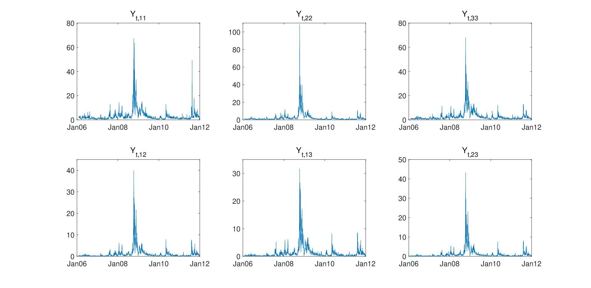

Figure 2 plots the diagonal and off-diagonal components of , exhibiting that has a clear clustering feature. Meanwhile, Figure 3 plots their sample autocorrelation functions (ACFs), which show the significant temporal dependence of . Based on these facts, we first fit by a diagonal VT-CBF model with , where the order is taken as one for ease of model identification, and the orders and are selected by the Bayesian information criterion (BIC). Specifically, this diagonal VT-CBF model is estimated using the two-step estimation procedure, and the corresponding estimates are give in Table 3. Second, since the sample ACFs of each component in Figure 3 decay slowly, we also fit by a diagonal VT-CBF-HAR model, and the related estimation results are also listed in Table 3. From this table, we find that the estimates of the degrees of freedom (especially for ) in both fitted models are close to each other, and both estimates of are small indicating the heavy-tailedness of the examined data. For the estimates of the mean parameter matrix , its standard errors based on the VT-CBF model are smaller than those based on the VT-CBF-HAR model. For other estimates of parameter matrices, the estimated diagonal components in each parameter matrix seem to have close values, meaning that the examined three stocks possibly have similar temporal structures. This similarity can also be seen from the values of persistence of each stock in Table 3, where the persistence of stock is defined by for the VT-CBF model and for the VT-CBF-HAR model. After estimation, we then apply our test statistics to both fitted models, and the results summarized in Table 4 imply that both fitted models are adequate at the 5% level.
| Diagonal VT-CBF model | ||||||||
|---|---|---|---|---|---|---|---|---|
| persistence | ||||||||
| 0.9771 | ||||||||
| 0.9788 | ||||||||
| 0.9762 | ||||||||
| Diagonal VT-CBF-HAR model | ||||||||
| persistence | ||||||||
| 0.9639 | ||||||||
| 0.9637 | ||||||||
| 0.9596 | ||||||||
- †
The asymptotic standard errors are given in the parenthesis.
| Diagonal VT-CBF model | Diagonal VT-CBF-HAR model | ||||||||||
|---|---|---|---|---|---|---|---|---|---|---|---|
| 2 | 3 | 4 | 5 | 6 | 2 | 3 | 4 | 5 | 6 | ||
| 1.494 | 4.170 | 8.004 | 9.428 | 11.513 | 4.385 | 6.127 | 7.004 | 10.310 | 11.583 | ||
| p-value | 0.474 | 0.244 | 0.091 | 0.093 | 0.074 | 0.112 | 0.106 | 0.136 | 0.067 | 0.072 | |
Next, we consider the forecasting performance of our proposed diagonal VT-CBF and VT-CBF-HAR models. Specifically, we compute the 1-step, 5-step and 10-step predictions of the RCOV matrices, based on a rolling window procedure with window size equal to . That is, for , we fit models based on observations , and forecast with and calculate the forecasting error by . To examine the importance of in the CBF models, we also apply the diagonal VT-CAW and VT-CAW-HAR models to do prediction for the purpose of comparison. The diagonal VT-CAW and VT-CAW-HAR models are defined in the same way as the diagonal VT-CAW and VT-CAW-HAR models, except that the matrix-F distribution for in the latter two models is replaced by the Wishart distribution. Besides the CAW-type models, we further include a diagonal VAR-HAR model for comparison, where this VAR model uses an HAR structure with the diagonal autoregressive parameter matrices to fit .
Table 5 gives the average of forecasting errors in Frobenius and spectral norms for all models. From this table, we can find that regardless of the prediction horizon, the diagonal VT-CBF-HAR model always has the smallest forecasting error in both norms. Moreover, we apply the DM test (Diebold and Mariano, 1995) to examine whether the diagonal VT-CBF-HAR model has a significant forecasting accuracy over other four competing models. The corresponding testing results are given in Table 5, and they show that the VT-CBF-HAR model is significantly better than its four competing models in terms of 5-step and 10-step forecasts. For 1-step forecasts, the VT-CBF-HAR and VT-CBF model models have comparable forecasting accuracy, and the VT-CBF-HAR model is significantly better than the remaining three models at level 10%. Note that the VAR-HAR model always performs worst in all examined cases, and this is probably because the VAR-HAR model brutally disentangles the matrix-structure of the RCOV matrices, which may have some intrinsic and useful value for forecasts.
| 1-step | 5-step | 10-step | ||||
|---|---|---|---|---|---|---|
| Diagonal Model | Frobenius | Spectral | Frobenius | Spectral | Frobenius | Spectral |
| VT-CBF-HAR | 1.5284 | 1.4607 | 1.9725 | 1.8850 | 2.2108 | 2.1091 |
| VT-CBF | 1.5349 | |||||
| VT-CAW-HAR | ||||||
| VT-CAW | ||||||
| VAR-HAR | ||||||
- 1
The DM test is used to compare the prediction accuracy between the diagonal VT-CBF-HAR and the other four competing models. The result of the each competing model is marked with “”, “” or “”, if the DM test implies the Diagonal VT-CBF-HAR model gives significantly more accurate predictions than this competing model at level 10%, 5% or 1%, respectively.
7.2 Application 2
In this section, we consider intra-day data of 112 stocks from four major sectors constituting S&P 500 index: 31 stocks from financial sector, 31 stocks from industrial sector, 25 stocks from health care sector, and 25 stocks from consumer discretionary sector, see Table 6. All intra-day price data are downloaded from Wharton Research Data Services (WRDS) database, and they are taken from 1 July, 2009 to 30 December, 2016, including 1890 non-missing dates of trading data in total.
| Number | Financial Sector | Industrial Sector | Health Care Sector | Consumer Discretionary Sector |
|---|---|---|---|---|
| 1 | AFL | BA | A | AZO |
| 2 | AIG | CAT | ABC | BBY |
| 3 | ALL | FLR | ABT | BWA |
| 4 | AXP | FLS | AET | CCL |
| 5 | BAC | GD | BAX | GPC |
| 6 | BBT | GE | BDX | GPS |
| 7 | BEN | GWW | BMY | HD |
| 8 | BK | HON | BSX | HRB |
| 9 | BLK | IR | CAH | JWN |
| 10 | C | ITW | CI | KMX |
| 11 | CMA | LLL | CVS | KSS |
| 12 | COF | LMT | HUM | LEG |
| 13 | GS | LUV | JNJ | LEN |
| 14 | HIG | MAS | LH | LOW |
| 15 | JPM | MMM | LLY | MCD |
| 16 | KEY | NOC | MCK | NKE |
| 17 | LNC | NSC | MDT | NWL |
| 18 | MCO | PH | MRK | PHM |
| 19 | MET | PNR | PFE | RL |
| 20 | MMC | PWR | PKI | TGT |
| 21 | MTB | RHI | SYK | TIF |
| 22 | PFG | ROK | TMO | TJX |
| 23 | PGR | ROP | UNH | VFC |
| 24 | PNC | RSG | VAR | WHR |
| 25 | PRU | RTN | WAT | YUM |
| 26 | RF | SNA | ||
| 27 | STI | SWK | ||
| 28 | STT | TXT | ||
| 29 | TMK | UNP | ||
| 30 | USB | UPS | ||
| 31 | WFC | UTX |
- 1
Note: Full names of selected stocks can be found in https://www.slickcharts.com/sp500
Based on 100 times log of the price data, the daily RCOV matrices are calculated by the TARVM method in Tao et al. (2011) for each sector.
For each sector, since the dimension of the RCOV matrix is large, we fit the RCOV matrix data by the diagonal F-VT-CBF and F-VT-CBF-HAR models. To do this, we first look for the value of in model (5.11) by plotting the ratios for each sector in Fig 4, where are the eigenvalues of in descending order. From Fig 4, we can choose for financial sector, for industrial sector, for health care sector, and for consumer discretionary sector. To get more information, we also plot the ratios for all four pooled sectors in Fig 5, from which is suggested. This implies that all 112 stocks considered may be driven by 3 latent factors, but among which only two may affect the industrial and health care sectors, and only one may affect the consumer discretionary sector. Hence, it is more reasonable to study the RCOV matrix data across sectors rather than together.


Next, we estimate the diagonal F-VT-CBF and F-VT-CBF-HAR models and choose the orders by a similar procedure as in Application 1, and the related results are reported in Table 7. From this table, we can find that except for the mean parameter matrix, the diagonal components of other parameter matrices seem to have different values, meaning that each component of has a different dynamical structure. Moreover, the values of persistence for show clear differences across four sectors, with the largest persistence in financial sector and the smallest persistence in health care sector. This finding indicates that the effect of past stock returns to its current volatility decays very slowly in the financial sector, while it behaves oppositely in the health care sector.
| Diagonal F-VT-CBF model | |||||||||||
| Sector | persistence | ||||||||||
| Financial | 0.9691 | ||||||||||
| 0.9903 | |||||||||||
| 0.9696 | |||||||||||
| Industrial | 0.9505 | ||||||||||
| 0.9300 | |||||||||||
| Health Care | 0.8841 | ||||||||||
| 0.8660 | |||||||||||
| Consumer Discretionary | 0.9467 | ||||||||||
| Diagonal F-VT-CBF-HAR model | |||||||||||
| Sector | persistence | ||||||||||
| Financial | 0.9618 | ||||||||||
| 0.9855 | |||||||||||
| 0.9491 | |||||||||||
| Industrial | 0.9406 | ||||||||||
| 0.8830 | |||||||||||
| Health Care | 0.8625 | ||||||||||
| 0.8130 | |||||||||||
| Consumer Discretionary | 0.9348 | ||||||||||
- †
The asymptotic standard errors given in the parenthesis are based on process rather than .
In the end, we examine the forecasting performance of our F-CBF models. As in Application 1, five different diagonal factor models (see Table 8) are considered to forecast , based on a rolling window procedure with window size equal to . Their forecasting performance is evaluated by the average of forecasting errors in Frobenius and spectral norms as well as the results of the related DM test in Table 8. From this table, we can see that except for the health care sector, the diagonal F-VT-CBF-HAR model always has the smallest forecasting error and the diagonal F-VAR-HAR model has the largest forecasting error. For 1-step forecasts in the health care sector, the diagonal F-VT-CAW-HAR has slightly smaller forecasting error compared with the diagonal F-VT-CBF-HAR model. In view of the results of DM test, the diagonal F-VT-CBF-HAR model has a significantly better performance than the other four competing models in terms of 5-step and 10-step forecasts, but this advantage is slightly weak in terms of 1-step forecasts, for which the diagonal F-VT-CBF and F-VT-CAW-HAR models have similar performance in the industrial sector, and the diagonal F-VT-CAW-HAR and F-VAR-HAR models have comparative performance in the health care sector.
| 1-step | 5-step | 10-step | ||||||
| Sector | Diagonal Model | Frobenius | Spectral | Frobenius | Spectral | Frobenius | Spectral | |
| Financial | F-VT-CBF-HAR | 8.7701 | 7.9339 | 10.4581 | 9.7229 | 11.0221 | 10.3200 | |
| F-VT-CBF | ||||||||
| F-VT-CAW-HAR | ||||||||
| F-VT-CAW | ||||||||
| F-VAR-HAR | ||||||||
| Industrial | F-VT-CBF-HAR | 7.9567 | 7.0936 | 9.3154 | 8.5480 | 9.8270 |
| |
| F-VT-CBF | ||||||||
| F-VT-CAW-HAR | ||||||||
| F-VT-CAW | ||||||||
| F-VAR-HAR | ||||||||
| Health Care | F-VT-CBF-HAR | 7.4977 | 6.8076 | 7.8436 | 7.1863 | |||
| F-VT-CBF | ||||||||
| F-VT-CAW-HAR | 6.6126 | 5.8559 | ||||||
| F-VT-CAW | ||||||||
| F-VAR-HAR | ||||||||
| Consumer Discretionary | F-VT-CBF-HAR | 8.3355 | 7.0130 | 9.3278 | 8.1225 | 9.6830 | 8.5081 | |
| F-VT-CBF | ||||||||
| F-VT-CAW-HAR | ||||||||
| F-VT-CAW | ||||||||
| F-VAR-HAR | ||||||||
- 1
The DM test is used to compare the prediction accuracy between the diagonal F-VT-CBF-HAR and the other four competing models. The result of the each competing model is marked with “”, “” or “”, if the DM test implies the Diagonal F-VT-CBF-HAR model gives significantly more accurate predictions than this competing model at level 10%, 5% or 1%, respectively.
8 Concluding Remarks
This paper proposes a new CBF model to study the dynamics of the RCOV matrix. For this CBF model, we explore its stationarity and moment properties, establish the asymptotics of its maximum likelihood estimator, and investigate the inner-product-based tests for its model checking. Hence, a systematic inferential tool of this CBF model is available for empirical researchers. In order to deal with large dimensional RCOV matrices, we also construct two reduced CBF models: the VT-CBF model and the F-CBF model. For both reduced models, the asymptotic theory of the estimated parameters is derived. Compared with the CAW model with Wishart innovations, the CBF model with matrix-F innovations is more able in capturing the heavy-tailed RCOV. This advantage is demonstrated by two real examples on U.S. stock markets. As motivated by Chiriac and Voev (2011), one obvious future work is to introduce the fractional integration structure into our CBF models. Another interesting potential future work could extend the idea of using the matrix-F innovation in a number of ways resulting in a large family of models, which shall be important to study the positive definite dynamics.
Supplementary Material
The online Supplementary Material contains the proofs of all theorems, and some useful derivatives.
References
- [1] Ahn, S. C. and Horenstein, A. R. (2013). Eigenvalue ratio test for the number of factors. Econometrica 81, 1203–1227.
- [2] Aït-Sahalia, Y. and Xiu, D. (2017). Using principal component analysis to estimate a high dimensional factor model with high-frequency data. Journal of Econometrics 201, 384–399.
- [3] Andersen, T. G., Bollerslev, T., Diebold, F. X. and Labys, P. (2003). Modeling and forecasting realized volatility. Econometrica 71, 579–625.
- [4] Barndorff-Nielsen, O. E. and Shephard, N. (2002). Econometric analysis of realized volatility and its use in estimating stochastic volatility models. Journal of the Royal Statistical Society: Series B 64, 253-280.
- [5] Barndorff-Nielsen, O. E. and Shephard, N. (2004). Econometric analysis of realized covariation: High frequency based covariance, regression, and correlation in financial economics. Econometrica 72, 885–925.
- [6] Barndorff-Nielsen, O. E., Hansen, P. R., Lunde, A. and Shephard, N. (2011). Multivariate realised kernels: consistent positive semi-definite estimators of the covariation of equity prices with noise and non-synchronous trading. Journal of Econometrics 162, 149–169.
- [7] Bauer, G. H. and Vorkink, K. (2011). Forecasting multivariate realized stock market volatility. Journal of Econometrics 160, 93–101.
- [8] Bollerslev, T. (1987). A conditionally heteroskedastic time series model for speculative prices and rates of return. Review of Economics and Statistics 69, 542–547.
- [9] Bollerslev, T., Engle, R. F. and Wooldridge, J. M. (1988). A capital asset pricing model with time-varying covariances. Journal of Political Economy 96, 116–131.
- [10] Bollerslev, T., Patton, A. J. and Quaedvlieg, R. (2016). Exploiting the errors: A simple approach for improved volatility forecasting. Journal of Econometrics 192, 1–18.
- [11] Boussama, F., Fuchs, F. and Stelzer, R. (2011). Stationarity and geometric ergodicity of BEKK multivariate GARCH models. Stochastic Processes and their Applications 121, 2331–2360.
- [12] Callot, L., Kock, A. and Medeiros, M. (2017). Modeling and forecasting large realized covariance matrices and portfolio choice. Journal of Applied Econometrics 32, 140–158.
- [13] Chiriac, R. and Voev, V. (2011). Modelling and forecasting multivariate realized volatility. Journal of Applied Econometrics 26, 922–947.
- [14] Comte, F. and Lieberman, O. (2003). Asymptotic theory for multivariate GARCH processes. Journal of Multivariate Analysis 84, 61–84.
- [15] Corsi, F. (2009). A simple approximate long-memory model of realized volatility. Journal of Financial Econometrics 7, 174–196.
- [16] Diebold, F. X. and Mariano, R. S. (1995). Comparing predictive accuracy. Journal of Business & Economic Statistics 13, 253–263.
- [17] Engle, R. F. (2002). Dynamic conditional correlation: A simple class of multivariate generalized autoregressive conditional heteroskedasticity models. Journal of Business & Economic Statistics 20, 339–350.
- [18] Engle, R. F. and Kroner, K. F. (1995). Multivariate simultaneous generalized ARCH. Econometric Theory 11, 122–150.
- [19] Engle, R. F. and Lee, G. (1999). A long-run and short-run component model of stock return volatility. Cointegration, Causality, and Forecasting: A Festschrift in Honour of Clive WJ Granger, 475–497.
- [20] Engle, R. F. and Mezrich, J. (1996). GARCH for groups. Risk 9, 36–40.
- [21] Fan, J., Qi, L. and Xiu, D. (2014). Quasi-maximum likelihood estimation of GARCH models with heavy-tailed likelihoods. Journal of Business & Economic Statistics 32, 178–191.
- [22] Francq, C., Horváth, L. and Zakoïan, J.-M. (2011). Merits and drawbacks of variance targeting in GARCH models. Journal of Financial Econometrics 9, 619–656.
- [23] Golosnoy, V., Gribisch, B. and Liesenfeld, R. (2012). The conditional autoregressive Wishart model for multivariate stock market volatility. Journal of Econometrics 167, 211–223.
- [24] Gouriéroux, C., Jasiak, J. and Sufana, R. (2009). The Wishart autoregressive process of multivariate stochastic volatility. Journal of Econometrics 150, 167–181.
- [25] Hafner, C. M. and Preminger, A. (2009). On asymptotic theory for multivariate GARCH models. Journal of Multivariate Analysis 100, 2044–2054.
- [26] Hansen, P. R., Huang, Z. and Shek, H. H. (2012). Realized GARCH: a joint model for returns and realized measures of volatility. Journal of Applied Econometrics 27, 877–906.
- [27] Jin, X. and Maheu, J. M. (2013). Modeling realized covariances and returns. Journal of Financial Econometrics 11, 335–369.
- [28] Jin, X. and Maheu, J. M. (2016). Bayesian semiparametric modeling of realized covariance matrices. Journal of Econometrics 192, 19–39.
- [29] Kim, D., Kong, X.-B., Li, C.-X. and Wang, Y. (2018). Adaptive thresholding for large volatility matrix estimation based on high-frequency financial data. Journal of Econometrics 203, 69–79.
- [30] Konno, Y. (1991). A note on estimating eigenvalues of scale matrix of the multivariate F-distribution. Annals of the Institute of Statistical Mathematics 43, 157–165.
- [31] Lam, C. and Yao, Q. (2012). Factor modeling for high-dimensional time series: Inference for the number of factors. Annals of Statistics 40, 694–726.
- [32] Leung, P. L. and Lo, M. (1996). An identity for the noncentral multivariate F distribution with application. Statistica Sinica 6, 419–431.
- [33] Li, D., Zhang, X., Zhu, K. and Ling, S. (2018). The ZD-GARCH model: A new way to study heteroscedasticity. Journal of Econometrics 202, 1–17.
- [34] Li, W. K. and McLeod, A. I. (1981). Distribution of the residual autocorrelations in multivariate ARMA time series models. Journal of the Royal Statistical Society: Series B 43, 231–239.
- [35] Ling, S. and Li, W. K. (1997). Diagnostic checking of nonlinear multivariate time series with multivariate ARCH errors. Journal of Time Series Analysis 18, 447–464.
- [36] Ling, S. and McAleer, M. (2003). Asymptotic theory for a vector ARMA-GARCH model. Econometric Theory 19, 280-310.
- [37] Lunde, A., Shephard, N. and Sheppard, K. (2016). Econometric analysis of vast covariance matrices using composite realized kernels and their application to portfolio choice. Journal of Business & Economic Statistics 34, 504–518.
- [38] McAleer, M. and Medeiros, M. C. (2008). Realized volatility: A review. Econometric Reviews 27, 10–45.
- [39] McCurdy, T. H. and Stengos, T. (1992). A comparison of risk-premium forecasts implied by parametric versus nonparametric conditional mean estimators. Journal of Econometrics 52, 225–244.
- [40] Noureldin, D., Shephard, N. and Sheppard, K. (2012). Multivariate high-frequency-based volatility (HEAVY) models. Journal of Applied Econometrics 27, 907–933.
- [41] Oh, D. H. and Patton, A. J. (2017). Modeling dependence in high dimensions with factor copulas. Journal of Business & Economic Statistics 35, 139–154.
- [42] Opschoor, A., Janus, P., Lucas, A. and Van Dijk, D. (2018). New HEAVY models for fat-tailed realized covariances and returns. Journal of Business & Economic Statistics 36, 643-657.
- [43] Pedersen, R. S. and Rahbek, A. (2014). Multivariate variance targeting in the BEKK-GARCH model. Econometrics Journal 17, 24–55.
- [44] Shen, K., Yao, J. and Li, W. K. (2018). Forecasting high-dimensional realized volatility matrices using a factor model. Forthcoming in Quantitative Finance.
- [45] Tao, M., Wang, Y., Yao, Q. and Zou, J. (2011). Large volatility matrix inference via combining low-frequency and high-frequency approaches. Journal of the American Statistical Association 106, 1025–1040.
- [46] Tao, M., Wang, Y. and Zhou, H. H. (2013). Optimal sparse volatility matrix estimation for high-dimensional Itô processes with measurement errors. Annals of Statistics 41, 1816–1864.
- [47] Tse, Y. K. (2002). Residual-based diagnostics for conditional heteroscedasticity models. Econometrics Journal 5, 358–374.
- [48] Wang, Y. and Zou, J. (2010). Vast volatility matrix estimation for high-frequency financial data. Annals of Statistics 38, 943–978.
- [49] Yu, P. L., Li, W. K. and Ng, F. C. (2017). The generalized conditional autoregressive Wishart model for multivariate realized volatility. Journal of Business & Economic Statistics 35, 513–527.
- [50] Zhu, K. and Li, W. K. (2015). A new pearson-type QMLE for conditionally heteroscedastic models. Journal of Business & Economic Statistics 33, 552–565.