ROBUST, FAST AND ACCURATE: A 3-STEP METHOD FOR
AUTOMATIC HISTOLOGICAL IMAGE REGISTRATION

In cancer diagnostics and histology related basic research, much insight into molecular and cellular interactions, tissue growth, and tissue organization is gained by analyzing consecutive but differently stained histological sections. For this procedure, a fixed tissue is transferred in a paraffin block and cut into $2-5\mu$m thin slices. Then, slices are subsequently stained by e.g. immunohistochemistry, and finally examined by a scientist or physician using conventional or virtual microscopy.

In order to correlate the staining intensities, staining patterns, and even subcellular localizations of various proteins or antigens, multiple stainings are frequently required. To recombine the information from the separate stains, a precise, multi-modal image registration is essential.

We present a 3-step registration pipeline that consists of 1) a robust pre-alignment, 2) a parametric registration computed on coarse resolution images, and 3) an accurate nonlinear registration.

The underlying variational image registration framework of this work has been described in [1, 2] and its application to histological images was first described in [3] in 2006. A general issue has been the handling of large images and the associated computational complexity and runtimes. At this time, the elastic registration of two images from slices of a human brain with $512\times 512$ pixels took about 100 minutes on a workstation and 3 minutes on a cluster computer. Later, a faster implementation for regular workstations reducing memory read and write operations has been proposed in [4] in 2013. The authors report a registration time of 104 seconds for a pair of images from the DIR-Lab 4DCT dataset (approx. $256\times 256\times 81$ voxels). Additional optimizations including the exploitation of special instruction sets of modern CPUs has been recently described in [5], reducing the registration time for two $256\times 256\times 256$ images to 19 seconds. The present work builds on top of these implementations.

Following the framework established by Fischer & Modersitzki [2], we formulate image registration as minimization of a suitable objective function $J(R,T,y)\rightarrow{\operatorname{min}}$, where $R:\mathbb{R}^{2}\mapsto\mathbb{R}$ and $T:\mathbb{R}^{2}\mapsto\mathbb{R}$ are the reference and template images and $y:\mathbb{R}^{2}\mapsto\mathbb{R}^{2}$ is the wanted transformation function. Central for any suitable objective function is a distance or image similarity measure that quantifies alignment quality. Here we use the Normalized Gradient Fields (NGF) distance measure [6]. In the discrete setting we assume we have 2D images composed from $N$ pixels with uniform size $h$ in each dimension and pixel centers $\mathbf{x}_{1},...,\mathbf{x}_{N}$. Thus, we use the NGF distance measure given by

with $\langle\mathbf{x},\mathbf{y}\rangle_{\varepsilon}=\mathbf{x}^{\top}\mathbf{y}+\varepsilon^{2}$, $\|\mathbf{x}\|_{\varepsilon}:=\sqrt{\langle\mathbf{x},\mathbf{y}\rangle_{\varepsilon}}$, and the edge parameter $\varepsilon$ steering the sensitivity with respect to strength of edges in images as well as to noise. The NGF distance measure forces the alignment of edges and therefore is based on morphological structures which makes it robust with respect to staining differences [7]. In general, NGF is suitable for multi-modal image registration.

Minimizing the NGF distance measure is part of all three steps that build up our registration pipeline. To solve the optimization problem we use a multilevel approach, starting with a low image resolution and refining the transformation on higher image resolutions iteratively. This reduces the risk of being tracked in local minima and speeds up the optimization process [8].

All three registration steps rely on the edge parameter $\varepsilon$, the number of levels $N_{\text{level}}$, the maximum image dimension in x and y for finest level $N_{\text{max}}$ and are set independently for each step.

Before registration, all images are converted into an in-house multilevel image format based on sqlite¹¹ 1 https://www.sqlite.org. Without this conversion, the image loading time is increased by about five seconds per registration.

In addition, all images are converted to gray and inverted while loading.

The algorithm has been applied to the data from the ANHIR registration challenge ²² 2 https://anhir.grand-challenge.org/Dataset [11, 12, 13]. The Registration performance is measured by evaluating the average ($\operatorname{AMrTRE}$) and the median ($\operatorname{MMrTRE}$) of the median relative target registration error ($\operatorname{MrTRE}$) over all image pairs $k=1,...,N_{\text{pairs}}$ following [11]. The $\operatorname{MrTRE}$ over all landmarks of one image pair $k$ is computed as

where $\mathbf{x}^{T},bfx^{W}$ are the template landmarks and the warped reference landmarks and $\mathbf{M}\in\mathbb{R}^{2}$ is the image extent. $\operatorname{AMrTRE}$ and $\operatorname{MMrTRE}$ are computed as the average and median

over the $\operatorname{MrTRE}$s of the image pairs. After registration, landmark errors for the training data $(N_{\text{pairs}}=230)$ of $\operatorname{AMrTRE}=0.49\%$ and $\operatorname{MMrTRE}=0.19\%$ are reached. On the subset of pairs where the registration is robust, landmarks errors of $\operatorname{AMrTRE}=0.30\%$ and $\operatorname{MMrTRE}=0.19\%$ are reached.

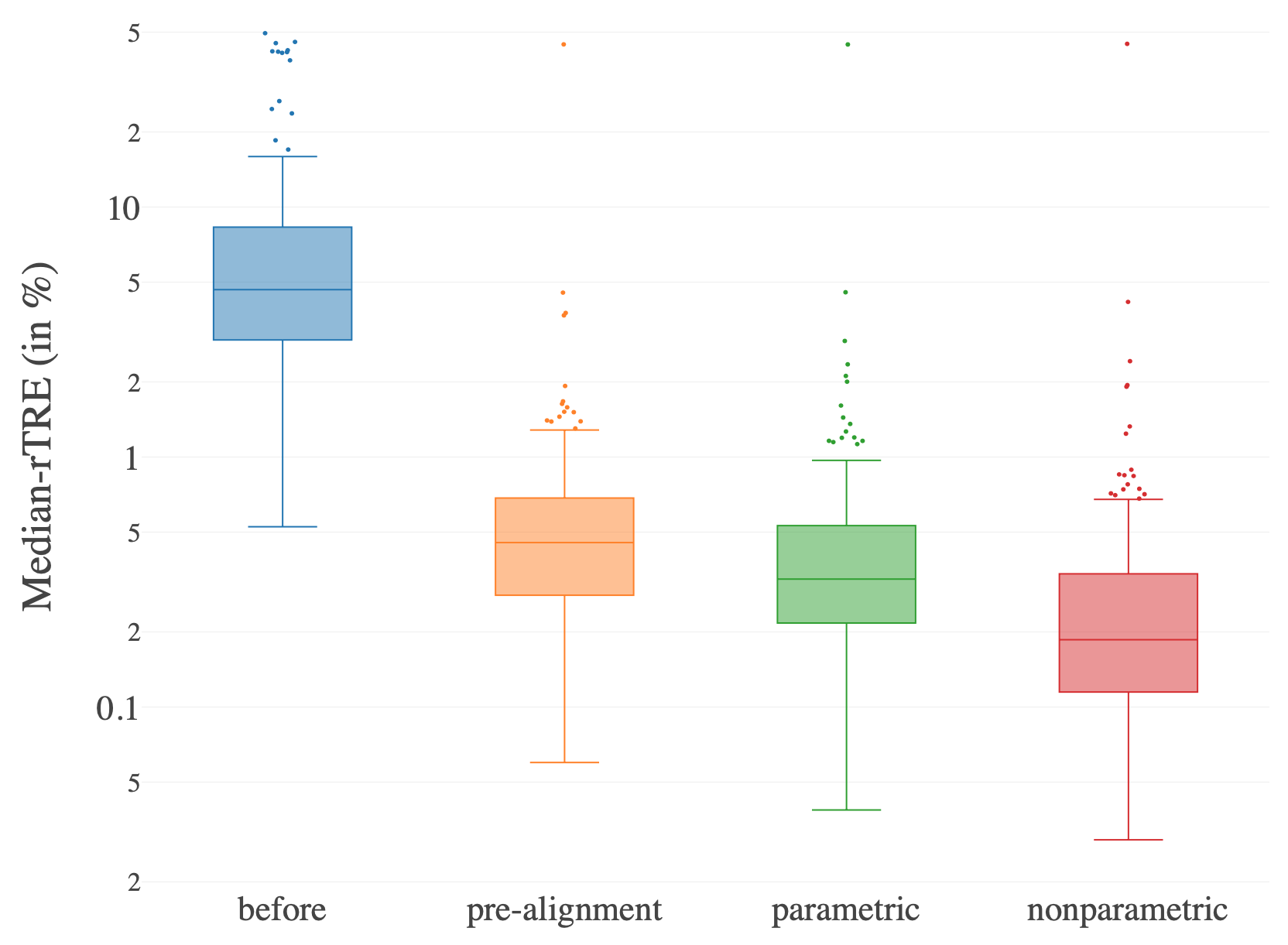
The reduction of the registration error in the training data after each step in the pipeline is shown in the box plots in Figure 2. While the median error is reduced after each step, those cases that fail in the pre-alignment cannot be recovered at a later stage. Figure 1 shows one of the image pairs after pre-alignment, parametric registration and non-parametric registration.

The resulting deformations do not contain foldings. The average maximum area change in one grid cell was 1.35 %.

The algorithm is robust in 99.6 % of the training cases $(N_{\text{pairs}}=230)$. Robustness in the ANHIR challenge is defined as the percentage of the cases where the landmark error is reduced compared to the initial configuration.

Multiple parametrizations were tested on the training data and the parameter set with the lowest median median rTRE (MMrTRE) was selected for submission.

The whole registration process including image loading, pre-alignment, parametric and non-parametric registration takes on average 4.0 seconds on an Intel(R) Core(TM) i7-7700K CPU (4.20GHz, four cores) with 32 GB of RAM.

References

- [1] Bernd Fischer and Jan Modersitzki, “Fast Image Registration - A Variational Approach,” in Numerical Analysis and Computational Mathematics, G Psihoyios, Ed., 2003, pp. 69–74.
- [2] Jan Modersitzki, FAIR: Flexible Algorithms for Image Registration, SIAM, 2009.
- [3] Oliver Schmitt, Jan Modersitzki, Stefan Heldmann, Stefan Wirtz, and Bernd Fischer, “Image Registration of Sectioned Brains,” International Journal of Computer Vision, vol. 73, no. 1, pp. 5–39, Sept. 2006.
- [4] Jan Rühaak, Stefan Heldmann, Till Kipshagen, and Bernd Fischer, “Highly Accurate Fast Lung CT Registration,” Proceedings of SPIE 8669, Medical Imaging 2013: Image Processing, Mar. 2013.
- [5] Lars König, Jan Rühaak, Alexander Derksen, and Jan Lellmann, “A Matrix-Free Approach to Parallel and Memory-Efficient Deformable Image Registration,” SIAM Journal on Scientific Computing, vol. 40, no. 3, pp. B858–B888, Jan. 2018.
- [6] E. Haber and J. Modersitzki, “Intensity Gradient Based Registration and Fusion of Multi-modal Images,” Methods of Information in Medicine, vol. 46, no. 03, pp. 292–299, 2007.
- [7] Wouter Bulten, “Epithelium segmentation using deep learning in H&E-stained prostate specimens with immunohistochemistry as reference standard,” Scientific Reports, vol. accepted, pp. 19, 2019.
- [8] Eldad Haber and Jan Modersitzki, “A Multilevel Method for Image Registration,” SIAM Journal on Scientific Computing, vol. 27, no. 5, pp. 1594–1607, 2006.
- [9] Millard F. Beatty, Principles of Engineering Mechanics, Number 32-33 in Mathematical Concepts and Methods in Science and Engineering. Plenum Press, New York, 1986.
- [10] Bernd Fischer and Jan Modersitzki, “Curvature based image registration,” Journal of Mathematical Imaging and Vision, pp. 81–85, 2003.
- [11] Jiri Borovec, Arrate Munoz-Barrutia, and Jan Kybic, “Benchmarking of Image Registration Methods for Differently Stained Histological Slides,” in 2018 25th IEEE International Conference on Image Processing (ICIP), Athens, Oct. 2018, pp. 3368–3372, IEEE.
- [12] Rodrigo Fernandez-Gonzalez, Arthur Jones, Enrique Garcia-Rodriguez, Ping Yuan Chen, Adam Idica, Stephen J. Lockett, Mary Helen Barcellos-Hoff, and Carlos Ortiz-De-Solorzano, “System for combined three-dimensional morphological and molecular analysis of thick tissue specimens,” Microscopy Research and Technique, vol. 59, no. 6, pp. 522–530, Dec. 2002.
- [13] Laxmi Gupta, Barbara Mara Klinkhammer, Peter Boor, Dorit Merhof, and Michael Gadermayr, “Stain independent segmentation of whole slide images: A case study in renal histology,” in 2018 IEEE 15th International Symposium on Biomedical Imaging (ISBI 2018), Washington, DC, Apr. 2018, pp. 1360–1364, IEEE.