Outlier-Robust Spatial Perception:
Hardness, General-Purpose Algorithms, and Guarantees
Abstract
Spatial perception is the backbone of many robotics applications, and spans a broad range of research problems, including localization and mapping, point cloud alignment, and relative pose estimation from camera images. Robust spatial perception is jeopardized by the presence of incorrect data association, and in general, outliers. Although techniques to handle outliers do exist, they can fail in unpredictable manners (e.g., RANSAC, robust estimators), or can have exponential runtime (e.g., branch-and-bound). In this paper, we advance the state of the art in outlier rejection by making three contributions. First, we show that even a simple linear instance of outlier rejection is inapproximable: in the worst-case one cannot design a quasi-polynomial time algorithm that computes an approximate solution efficiently. Our second contribution is to provide the first per-instance sub-optimality bounds to assess the approximation quality of a given outlier rejection outcome. Our third contribution is to propose a simple general-purpose algorithm, named adaptive trimming, to remove outliers. Our algorithm leverages recently-proposed global solvers that are able to solve outlier-free problems, and iteratively removes measurements with large errors. We demonstrate the proposed algorithm on three spatial perception problems: 3D registration, two-view geometry, and SLAM. The results show that our algorithm outperforms several state-of-the-art methods across applications while being a general-purpose method.
I Introduction
Spatial perception is concerned with the estimation of a geometric model that describes the state of the robot, and/or the environment the robot is deployed in. As such, spatial perception includes a broad set of robotics problems, including motion estimation [1], object detection, localization and tracking [2], multi-robot localization [3], dense reconstruction [4], and Simultaneous Localization and Mapping (SLAM) [5]. Spatial perception algorithms find applications beyond robotics, including virtual and augmented reality, and medical imaging [2], to mention a few.
| (a) 3D registration |
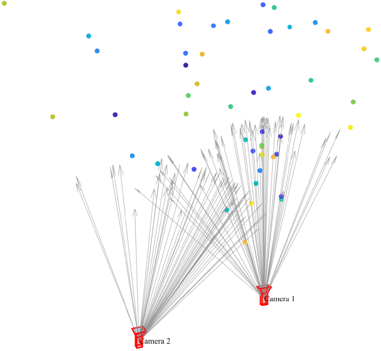 (b) Two-view geometry
|
 (c) 2D SLAM
|
 (d) 3D SLAM
|
Safety-critical applications, including self-driving cars, demand robust spatial perception algorithms that can estimate correct models (and assess their performance) in the presence of measurement noise and outliers. While we currently have several approaches that can tolerate large measurement noise (e.g., [6, 7, 8]), these algorithm tend to catastrophically fail in the presence of outliers resulting from incorrect data association, sensor malfunction, or even adversarial attacks.
In this paper, we focus on the analysis and design of outlier-robust general-purpose algorithms for robust estimation applied to spatial perception. Our proposal is motivated by three observations. First, recent years have seen a convergence of the robotics community towards optimization-based approaches for spatial perception. Therefore, despite the apparent heterogeneity of the perception landscape, it is possible to develop general-purpose methods to reject outliers (e.g., M-estimators [9] and consensus maximization [10] can be thought as general estimation tools). Second, the research community has developed global solutions to many perception problems without outliers, from well-established techniques for point cloud registration [8], to very recent solvers for SLAM [6] and two-view geometry [7]. These global solvers offer unprecedented opportunities to tackle robust estimation with outliers. Third, the literature still lacks a satisfactory answer to provably-robust spatial perception.
The literature on outlier-robust spatial perception is currently divided between fast approaches (that mainly work in the low-outlier regime, without performance guarantees) and provably-robust approaches (that can tolerate many outliers, but have exponential run-time). While we postpone a comprehensive literature review to Section VII, it is instructive to briefly review this dichotomy. Fast approaches include RANSAC [11], M-estimators [9], and measurement-consistency checking [12, 13]. These methods fall short of providing performance guarantees. In particular, RANSAC is known to become slow and brittle with high outlier rates () [10], and does not scale to high-dimensional problems, while M-estimators have a breakdown point of zero, meaning that a single “bad” outlier can compromise the results. On the other hand, provably-robust methods, typically based on branch-and-bound [14, 15, 16, 17, 10], can tolerate more than of outliers [18], but do not scale to large problems and are relatively slow for robotics applications. Overall, the first goal of this paper is to understand whether we can resolve this divide, and design algorithms that are both efficient and provably robust.
Contributions. We propose a Minimal Trimmed Squares (MTS) formulation for outlier-robust estimation. MTS encapsulate a wide spectrum of commonly-used outlier-robust formulations in the literature, such as the popular maximum consensus [19], Linear Trimmed Squares [20], and truncated least-squares [21]. In particular, MTS aims to compute a “good” estimate by rejecting a minimal set of measurements.
Our first contribution (Section III) is a negative result: we show that outlier rejection is inapproximable. In the worst-case, there exist no quasi-polynomial algorithm that can compute (even an approximate) solution to the outlier rejection problem. We prove that this remains true, surprisingly, even if the algorithm knows the true number of outliers and even if we allow the algorithm to reject more measurements than necessary. Our conclusions largely extend previously-known negative results [19], which already ruled-out the possibility of designing polynomial-time approximation methods.
Our second contribution (Section IV) is to derive the first per-instance sub-optimality bounds to assess the quality of a given outlier rejection solution. While in the worst case we expect efficient algorithms to perform poorly, we can still hope that in typical problem instances a polynomial-time algorithm can compute good solutions, and we can use the proposed sub-optimality bounds to assess the performance of such an algorithm. Our bounds are algorithm-agnostic (e.g., they also apply to RANSAC) and can be computed efficiently.
Our third contribution (Section V) is a general-purpose algorithm for outlier rejection, named Adaptive Trimming (ADAPT). ADAPT leverages recently-proposed global solvers that solve outlier-free problems and adaptively removes measurements with large residual errors. Despite its simplicity, our experiments show that it outperforms RANSAC and even specialized state-of-the-art methods for robust estimation.
We conclude the paper by providing an experimental evaluation across multiple spatial perception problems (Section VI). The experiments show that ADAPT can tolerate up to 90% outliers in 3D registration (with a run-time similar to existing methods), and up to 50% outliers in two-view geometry and most SLAM datasets. The experiments also show that the proposed sub-optimality bounds are effective in assessing the outlier rejection outcomes. We report extra results and proofs in the Appendix.
II Outlier Rejection: a Minimally Trimmed Squares Formulation
Many estimation problems in robotics and computer vision can be formulated as non-linear least squares problems:
| (1) |
where we are given measurements of an unknown variable , with ( is the measurement set), and we want to estimate , potentially restricted to a given domain (e.g., is a pose, and is the set of 3D poses). The least squares problem in eq. (1) looks for the that minimizes the (squares of) the residual errors , where the -th residual error captures how well explains the measurement . The problem in eq. (1) typically results from maximum likelihood and maximum a posteriori estimation [5, 22], under the assumption that the measurement noise is Gaussian.
Both researchers and practitioners are well-aware that least squares formulations are sensitive to outliers, and that the estimator in eq. (1) fails to produce a meaningful estimate of in the presence of gross outliers . Therefore, in this paper we address the following question:
Can we compute an accurate estimate of that is insensitive to the presence of outlying measurements?
We formulate the resulting robust estimation problem as the problem of selecting a small number of outliers, such that the remaining measurements (the inliers) can be explained with small error. In other words, a good estimate (in the presence of outliers) is one that explains as many measurements as possible while disregarding outliers. This intuition leads to the following formulation.
Problem 1 (Minimally Trimmed Squares (MTS))
Let denote a set of measurements of an unknown variable , and let denote the -th measurement. Also denote with the residual error that quantifies how well fits the measurement . Then, the minimally trimmed squares problem consists in estimating the unknown variable by solving the following optimization problem:
| (2) |
where one searches for the smallest set of outliers ( is the cardinality of a set) among the given measurements , such that the remaining measurements (i.e., the inliers) can be explained with small error, i.e., for some , and where is a given outlier-free bound.
Example 1 (Robust linear estimation and bound )
In linear estimation one wishes to recover a parameter from a set of noisy measurements , , where is a known vector, and models the unknown measurement noise. Some of the measurements (the inliers) are such that the corresponding noise can be assumed to follow a Gaussian distribution, while others (the outliers) may be affected by large noise. Therefore, our MTS estimator can be written as:
| (3) |
Evidently, must increase with the number of inliers, since each inlier adds a positive summand due to the presence of noise. Moreover, since the sum is restricted to the inliers, for which the noise is assumed to be Gaussian, we can compute the desired outlier-free bound explicitly: if follows a Gaussian distribution, then each follows a distribution with degree of freedom. Thus, with desired probability (e.g., ), where is the -quantile of the distribution, and the outlier-free bound is .
Remark 2 (Generality and applicability)
In this paper we address robustness in non-linear and non-convex estimation problems as the ones arising in robotics and computer vision. Therefore, while the linear estimation Example 1 is instructive (and indeed we will prove in Section III that even in such a simple case, it is not possible to even approximate the MTS estimator in polynomial time), the algorithms and bounds presented in this paper hold for any function and any domain . In contrast with related work [23, 24], we do not assume the number of outliers to be known in advance (an unrealistic assumption in perception problems). Indeed, our MTS formulation looks for the smallest set of outliers. Finally, while the formulation (2) requires to set an outlier-free threshold, we will propose an algorithm (Section V) that will automatically compute a suitable threshold without any prior knowledge about the measurement noise.
In summary, MTS is a general non-linear and non-convex outlier rejection framework. We exemplify its generality by discussing its application to three core perception problems: 3D registration, two-view geometry, and SLAM.
II-A Outlier rejection for robust spatial perception:
3D registration, two-view geometry, and SLAM
Here we review three core problems in spatial perception, and show how to tailor the framework of Section II to these examples. The expert reader can safely skip this section.
Outlier rejection for 3D registration. Point cloud registration consists in finding the rigid transformation that aligns two point clouds. Formally, we are given two sets of points and (with , for ), as well as a set of putative correspondences , such that the point and the point are (putatively) related by a rigid transformation, for all . Point correspondences are typically obtained by descriptor matching [18].
Given the points and the putative correspondences, 3D registration looks for a rotation , and a translation , that align (i.e., minimize the sum of the squared distances between) corresponding points:
| (4) |
The problem in eq. (4) can be solved in closed form [8]. However, eq. (4) fails to produce a reasonable pose (rotation and translation) estimate when some of the correspondences are outliers [18, 25], and related work resorts to robust estimators (reviewed in Section VII). Here we rephrase robust registration as an MTS problem:
| (5) |
Outlier rejection for two-view geometry. Two-view geometry estimation consists in finding the relative pose (up to scale) between two camera images picturing a static scene, and it is crucial for motion estimation [26], object localization [26], and reconstruction [27, Chapter 1]. We consider a feature-based calibrated setup where the camera calibration is known and one extracts features (keypoints) and from the first and second image, respectively. We are also given a set of putative correspondences between pairs of features , such that features and (putatively) picture the same 3D point observed in both images.
Given the features and the putative correspondences, two-view geometry looks for the rotation and the translation (up to scale) that minimizes the violation of the epipolar constraint:
| (6) |
where is restricted to the unit sphere to remove the scale ambiguity. In the absence of outliers, problem (6) can be solved globally using convex relaxations [7].
In the presence of outliers, the non-robust formulation in eq. (6) fails to compute accurate pose estimates, hence we rephrase two-view estimation as an MTS problem:
| (7) |
Outlier rejection for SLAM. Here we consider one of the most popular SLAM formulations: Pose graph optimization (PGO). PGO estimates a set of robot poses () from pairwise relative pose measurements between pairs of poses . The measurement set includes odometry (ego-motion) measurements as well as loop closures. In the absence of outliers, one can compute the pose estimates as:
| (8) |
where denotes the Frobenius norm.
In practice, many loop closure measurements are outliers (e.g., due to failures in place recognition). Therefore, we rephrase PGO as an MTS problem over the loop closures:
| (9) |
where we split the measurement set into odometric edges (these can be typically trusted), and loop closures (typically containing outliers).
III Outlier Rejection is Inapproximable
We show that MTS is inapproximable even by quasi-polynomial-time algorithms. To this end, we find worst-case instances for which there is no algorithm that can reject a few measurements to achieve a prescribed residual error (subject to a widely believed conjecture in complexity theory, similar to ). We start with some definitions and present our key result in Theorem 5.
Definition 3 (Approximability)
Consider the MTS Problem 1. Let be an optimal solution, let , and , that is, is the outlier-free bound when the measurements are the rejected outliers. Also, consider a number . We say that an algorithm makes MTS -approximable if it returns a set , and a parameter , such that and .
The definition of -approximability allows some slack in the quality of the MTS’s solution: rather than solving Problem (2) exactly (), Definition 3 only requires, for MTS to be approximable, to find an algorithm that computes an estimate close to the optimal solution. Indeed, Definition 3 includes algorithms that can reject more outliers than necessary (since ).
Definition 4 (Quasi-polynomial algorithm)
An algorithm is said to be quasi-polynomial if it runs in time, where is the size of the input and is constant.
Any polynomial algorithm is also quasi-polynomial, since . Yet, a quasi-polynomial algorithm is asymptotically faster than an exponential-time algorithm, since exponential algorithms run in time, for some .
Theorem 5 (Inapproximability)
Consider the linear MTS problem (3). Let be the optimal value of the variable to be estimated, be the number of measurements (), be the optimal solution, and set . Then, for any , there exist a polynomial and a and instances of MTS (i.e., measurements , vectors , and outlier-free bound ) where , such that unless ,11 1 The complexity hypothesis means there is no randomized algorithm which outputs solutions to problems in with probability , after running for time, for a constant [28]. there is no quasi-polynomial algorithm making MTS -approximable. This holds true even if the algorithm knows , and that exist.
Theorem 5 stresses the extreme hardness of MTS. Even if we inform the algorithms with the true number of outliers, it is impossible in the worst-case for even quasi-polynomial algorithms to find a good set of inliers. Surprisingly, this remains true even if we allow the algorithms to cheat by rejecting more measurements than (i.e., ).
Thinking beyond the worst-case, our inapproximability result suggests that to obtain a good solution efficiently, our only hope is that nature (which picks the outliers) is not adversarial, thus fast algorithms can compute good solutions in practice. Hence, it becomes important to derive per-instance bounds that, for a given MTS problem (i.e., given , and in (1)), can evaluate how far an algorithm is from the optimal MTS solution. In order words, since we cannot guarantee than any efficient algorithm will do well in the worst-case, we are happy with evaluating (a posteriori) if an algorithm computed a good solution for a given problem instance. For this reason, in the next section we develop the first per-instance sub-optimality bound for Problem 1.
IV Performance Guarantees
We present the first per-instance (i.e., a posteriori) sub-optimality bound for the MTS Problem 1. The bound is algorithm-agnostic (does not take assumption on the way is generated), and is computable in time. Also, we demonstrate its informativeness via simulations.
Theorem 6 (A posteriori sub-optimality bound)
Consider the MTS problem (2) and let be an optimal solution to (2). Also, for any candidate solution , let:
- •
; i.e., is the minimum residual error given the rejection ;
- •
; i.e., is the optimal residual error when at most measurements are rejected;
- •
; i.e., is the residual error for the optimal outlier rejection .
Then, given a candidate solution , the following bound relates the residual error of the candidate solution with the residual error of an optimal solution rejecting the same number of outliers:
| (10) |
where
| (11) |
Moreover, if it is also known that , then it holds:
| (12) |
Eq. (10) quantifies the distance between the residual of the candidate solution and the residual of an optimal solution rejecting the same number of outliers . Intuitively, if we incorrectly pick outliers and obtain a residual error , there might exist a more clever selection that instead obtains ; on the other hand, we would like and to be as close as possible. For this reason, the smaller , the closer the candidate selection is to the optimal selection. For example, when , then , i.e., we conclude that the algorithm returned a globally optimal solution (restricted to the ones rejecting measurements).
Eq. (12) completes the picture by stating that if the algorithm rejects at least as many measurements as the optimal solution (), then the bound in eq. (12) compares the quality of directly with the optimal residual error of , the optimal solution of the MTS Problem 1.
Remark 7 (Quality of the bound)
We showcase the quality of the bound (11) by considering the linear estimation Example 1. We generate small instances for which we can compute the optimal solution and evaluate the corresponding residual error . In particular, we compute the optimal solution using CPLEX [30], a popular library for mixed-integer linear programming, and we compare the optimal solution against a candidate solution . We generate candidate solutions using a greedy algorithm [29]. The greedy algorithm, at each iteration, rejects the measurement that induces the largest decrease in the residual error. Fig. 2 shows in blue the actual (true) approximation performance of the greedy algorithm () and in red the bound in eq. (10). The results are averaged over 10 Monte Carlo simulations. The figure shows that the bound predicts well the actual sub-optimality ratio (note the scale of the -axis) and its quality improves for increasing number of outliers.
We remark that the bound (11) can be also used to quantify the performance of existing algorithms, including RANSAC. Having introduced our per-instance sub-optimality bounds, we step forward to a novel general-purpose algorithm for outlier rejection that empirically returns accurate solutions (and for which our bound is typically close to zero).
V A General-Purpose Algorithm: ADAPT
-
[leftmargin=-.5cm,label=•]
- 1.
: minimum nr. of measurements required by global solver;
- 2.
: discount factor for outlier threshold (default );
- 3.
: convergence threshold;
- 4.
: nr. of iterations to decide convergence (default );
- 5.
: maximum nr. of extra rejections per iteration.
We introduce a novel algorithm for outlier rejection that we name Adaptive Trimming (ADAPT). The algorithm starts by processing all measurements and at each iteration it trims measurements with residuals larger than a threshold. It is adaptive in that it dynamically decides the threshold at each iteration (hence relaxing the need for a threshold ). Moreover, it is not greedy in that it can reject multiple measurements at each iteration while it keeps revisiting the quality of previously rejected outliers.22 2 In our tests we found that a greedy algorithm similar to [29] tends to converge to poor outlier rejection decisions and is typically slow for practical applications, since it has quadratic runtime in the number of measurements.
Assumption 8 (Global solver)
ADAPT assumes the availability of a black-box solver that can (even approximately) solve the outlier-free problem (1) to optimality.
Luckily, for all problems in Section II-A, there exist (outlier-free) global solvers, including [6, 7, 8].
Description of ADAPT. The preudo-code of ADAPT is given in Algorithm 1. Here, we use the additional notation:
- •
Let ; i.e., is an estimator of given an outlier selection .
- •
Let ; i.e., is the residual of the measurement , given an outlier selection .
Per Algorithm 1, ADAPT executes five distinctive operations:
Initialization (line 1)
ADAPT initializes the iteration counter and the current candidate outlier set with the empty set. It also initializes , the outlier group size, which constrains the maximum number of measurements that can be deemed as outliers in a single iteration of the algorithm. Moreover, ADAPT initializes the counter : this is used to decide whether convergence has been reached. Finally, it initializes the outlier threshold with the value of the largest residual across all measurements. Note that computing (for any ) requires calling the global solver on the measurements , and then evaluating the residual errors for all measurements in .
Outlier set update (lines 5-6)
Given the current threshold and group size , the algorithm updates the outlier set in two steps: first (line 5), it finds the set of measurements with the largest residuals among all measurements in ;33 3 Note that the selection is performed over all measurements , potentially revisiting measurements that were previously deemed to be outliers. second (line 6), the algorithm updates the outlier set as the collection of all the measurements in whose residual exceeds the outlier threshold .
Outlier threshold update (lines 7-8)
Outlier group size update (line 9)
After each iteration , ADAPT increases the outlier group size by . This has the effect of increasing the maximum number of measurements that can be deemed as outliers in future iterations: intuitively, ADAPT is conservative in rejecting measurements at the beginning (small initial ) , while it gets more and more aggressive by gradually increasing .
Termination
ADAPT terminates when one of the following two conditions is satisfied. First (lines 10-11), it may terminate when all but a number of measurements have been rejected, where is the minimum number of measurement that the global solver needs to solve the problem (for example, in 3D registration, ). Second (lines 14-15), ADAPT may terminate if convergence has been achieved. In particular, if the algorithm observes for consecutive times that the absolute value of the residuals function changes by less than , then it terminates ( counts the number of consecutive times a decrease smaller than is observed).
Remark 9 (Complexity and practicality)
The termination condition in line 10 guarantees the termination of the algorithm with at most calls of the global solver. ADAPT terminates faster as one increases the outlier group size , the convergence thresholds , and/or as one decreases the discount factor and the number of iterations to decide convergence. Overall, the linear runtime (in the number of measurements) of ADAPT makes the algorithm practical in real-time applications where fast global solvers are available.
Remark 10 (vs. RANSAC)
While RANSAC builds an inlier set by sampling small (minimal) sets of measurements, ADAPT iteratively prunes the overall set of measurements. Arguably, this gives ADAPT a “global vision” of the measurement set as we showcase in the experimental section. RANSAC assumes the availability of fast minimal solvers, while ADAPT assumes the availability of fast global (non-minimal) solvers. Finally, RANSAC is not suitable for high-dimensional problems where is becomes exponentially more difficult to sample an outlier-free set [18]. On the other hand, ADAPT is deterministic and guaranteed to terminate in a number of iterations bounded by the number of measurements.
VI Experiments and Applications
We evaluate ADAPT against the state of the art in three spatial perception problems: 3D registration (Section VI-A), two-view geometry (Section VI-B), and SLAM (Section VI-C). The results show that ADAPT outperforms RANSAC in terms of accuracy and scalability, and often outperforms specialized outlier rejection methods (in particular for SLAM) while being a general-purpose algorithm. Finally, the tests show that the performance bounds of Section IV are informative and can be used to assess the outlier rejection outcomes. All results are averaged over 10 Monte Carlo runs.
VI-A Robust Registration
| (a) Rotation Error |
| (b) Translation Error |
Experimental setup. We test ADAPT on two standard datasets for 3D registration: the Stanford Bunny and the ETH Hauptgebaude [31]. In both cases we downsample the point clouds obtaining 453 points for Bunny and 3617 points for ETH. For each point cloud we generate a second point cloud by applying a random rigid transformation and adding noise and outliers. The (inlier) noise standard deviation is set to 0.025% and 0.05% of the point cloud diameter respectively. Outliers are generated by replacing a subset of the points in with random points uniformly sampled in the bounding box containing . In each iteration, ADAPT uses Horn’s method [8] as global solver. We benchmark ADAPT against Fast Global Registration (FGR) [25] and the three-point RANSAC. We set the maximum number of iterations in RANSAC to 1000 and use default parameters for FGR. All methods are implemented in MATLAB.
Results. Fig. 3 shows the (average) translation and rotation errors for the estimates computed by ADAPT, FGR, and RANSAC on the Bunny dataset for increasing outlier percentages. ADAPT performs on-pair with FGR which is a specialized robust solver for 3D registration and they both achieve practically zero error for up to 90% of outliers, after which they both break. RANSAC starts performing distinctively worse early on and is dominated by the other techniques (after 90% all techniques fail to provide a satisfactory estimate). We obtain similar results on the ETH dataset hence for space reasons we report them in Appendix C.
For both the Bunny and ETH datasets, we compute the sub-optimality bound for the result of ADAPT, using Theorem 6. The plot of the bound is given in Appendix C; the bound remains around , confirming that ADAPT remains close to the optimal outlier selection. The runtime of ADAPT is comparable to FGR and is reported in Appendix C.
VI-B Robust Two-view Geometry
| (a) Rotation Error |
| (b) Translation Error |
Experimental setup. We tested ADAPT on both synthetic data and on the MH_01 sequence of the EuRoC dataset [32]. To generate the synthetic data we place the first camera at the origin (identity pose) and place the second camera randomly within a bounded region. Then, we generate a random point cloud within the field-of-view of both camera. The points projected on the camera frame are finally corrupted with Gaussian noise, and outliers are added. For the EuRoC dataset, we extract Harris corners in each frame and track keypoints in consecutive frames using Lucas-Kanade feature tracking as in [33]; the results are then averaged across all pairs of consecutive frames in the sequence. In each iteration, ADAPT uses Briales’ QCQP relaxation [7] as global solver. We benchmarked ADAPT against Nister’s five-point [26] and the eight-points algorithm [34] within RANSAC.
Results. Fig. 4 shows the box-plot of translation and rotation errors for the estimates of ADAPT, the five- and eight-point RANSAC on the synthetic dataset. ADAPT outperforms the other techniques across all the spectrum. ADAPT and five-point perform on-pair till 40% of outliers. Beyond that point, the five-point method attains considerably higher errors than ADAPT (50% to 100% more in rotation; and more than 300% more in translation). The eight-point method results in higher errors than the five-point across the spectrum.
Fig. 5 shows the results on the EuRoC dataset focusing on the comparison between ADAPT and the five-point RANSAC. ADAPT achieves a mean rotation error of rad versus rad of the five-point. Similarly for the translation error: 0.075m for ADAPT versus 0.09m for the five-point. For visualization purposes we cut the translation box-plot in Fig. 5 above 0.25m error: in reference to the rest of the plot, we report that ADAPT exhibits translation errors larger than in 10% of the frames, whereas only of the five-point estimates have translation errors larger than .
For the synthetic dataset, the typical value for the sub-optimality bound achieved by ADAPT is . That is, ADAPT makes a rejection that achieves an error that is at most 20% away from the optimal, even in the presence of 90% of outliers. The runtime of ADAPT is reported in Appendix C: our approach is one order of magnitude slower than the five-point method, mainly due to the relatively high runtime of the global solver [7], which is called in each iteration.
VI-C Robust SLAM
 (a) MIT
|
 (b) CSAIL
|

|
Experimental setup. We test ADAPT on standard 2D and 3D SLAM benchmarking datasets and report extra results on synthetic datasets in Appendix C. We spoil existing datasets with spurious loop closures: we sample random pairs of nodes and we add an outlier relative pose measurement between them, where the relative translation is sampled in the ball of radius 5m and the rotation is sampled uniformly at random in or . The ground truth trajectory is generated by optimizing the problem with SE-Sync [6] before adding outliers. We also use SE-Sync as the global solver for ADAPT. We test the following datasets, described in [35, 6]: MIT (2D), Intel (2D), CSAIL (2D), and Sphere2500 (3D). We also test a simulated 3D grid dataset (results in Appendix C). We benchmark ADAPT against DCS [36]; we report DCS results for three choices of the robust kernel size: {1,10,100} (the default value is 1, see [36]).
Results. ADAPT outperforms DCS (independently on the choice of the kernel size) across all outlier percentages.
2D SLAM: In the MIT dataset (Fig. 6a), a particularly challenging dataset, ADAPT is insensitive to up to 20% of outliers. All variants of DCS fail to produce an error smaller than 10 meters even in the absence of outliers: DCS is an iterative solver, hence is may converge to local minima when bootstrapped from a bad initial guess (the odometric estimate is particularly noisy in MIT). ADAPT leverages SE-sync, which is a global solver, hence is able to converge to the correct solution. In the CSAIL dataset (Fig. 6b), ADAPT also dominates DCS while DCS performance is acceptable when the kernel size is equal to 100. Unfortunately, the choice of a “good” kernel size is dataset-dependent and it can make the difference between an adequate performance in DCS and a catastrophic failure. ADAPT also dominates DCS in the INTEL dataset, whose statistics are reported in Appendix C.
3D SLAM: In the Sphere dataset (Fig. 7), ADAPT achieves and error below 0.25m across all outlier percentages. On the other hand, DCS starts with an error of 0.25 meters (0% outliers) and ends up with at least 2.5 meters error (50% outliers). Again, ADAPT, a general-purpose approach for outlier rejection, outperforms specialized techniques for robust SLAM. Appendix C also reports similar conclusions and results for the 3D grid dataset.
For 2D SLAM, the typical value for the sub-optimality bound achieved by ADAPT, per Theorem 6, is 0.1 (MIT) and 0.01 (Intel and CSAIL) across all spectrum of outlier percentages. For 3D SLAM, the typical value of the bound achieved by ADAPT is 0.1 (3D grid) and 0.01 (sphere).
ADAPT is one to two orders slower than DCS. This is due to the repeated calls to SE-sync and is further aggravated in the 3D case by the fact that SE-sync tends to be slow in the presence of outliers (the Riemannian staircase method [6] requires multiple staircase iterations since the rank of the relaxation increases in the presence of outliers).
VII Related Work
We extend the literature review in Section I, across robotics and computer vision (Section VII-A), and statistics and control (Section VII-B), as well as, across sub-optimality guarantees in outlier-robust estimation (Section VII-C).
VII-A Outlier-robust estimation in robotics and computer vision
Outlier-robust estimation is an active research area in robotics and computer vision for decades [37, 38, 9]. Traditionally, low-dimensional problems are solved using RANSAC [11] (e.g., 3D registration, and two-view geometry). RANSAC is efficient and effective for low outlier rates [10]. However, the need to cope with higher outlier rates pushed research towards global optimization methods, such as branch-and-bound (BnB) [14, 15, 16, 17, 10], and mixed-integer programming (MIP) [39]. Nevertheless, for high-dimensional problems (e.g., SLAM), RANSAC, BnB, and MIP are typically slow to be practical: in the worst-case, they require exponential run-time. Hence, research has also focused on M-estimators, in conjunction with either non-convex optimization [40, 36, 41], or convex relaxations [42], possibly also including decision variables for the outlier rejection [43, 42, 40, 36]. In more detail, representative outlier-robust methods for 3D registration, two-view geometry, and SLAM are the following.
Robust 3D registration. The goal is to find the transformation (translation and rotation) that aligns two point clouds. In the presence of outliers, created by incorrect point correspondences, one typically resorts to RANSAC [44, 11], along with a 3-point minimal solver —the outlier-free problem admits well-known closed form solutions [45, 8]. But when the outliers’ number is more than 50%, RANSAC tends to be slow, and brittle [10, 18]. Thereby, recent approaches adopt either robust cost functions [46, 9, 25], or BnB [24, 47, 18]: Zhou et al. [25] propose fast global registration (FGR), which is based on the Geman-McClure robust cost function; Yang et al. [24] propose a approach; Campbell et al. [47] employ BnB to search the space of camera poses, guaranteeing global optimality without requiring a pose prior; and Bustos et al. [18] add a pre-processing step, that removes gross outliers before RANSAC or BnB. Other approaches, that iteratively compute point correspondences, include iterative closest point (ICP) [48, 49], and trimmed iterative closest point algorithm [50]; all require an accurate initial guess [25].
Robust two-view geometry. The problem consists in estimating the relative pose (up to scale) between two images, given pixel correspondences. In robotics, RANSAC is again the go-to approach [1], typically in conjunction with Nister’s 5-point method [51], a minimal solver —other minimal solvers exist when one is given a reference direction [52], the relative rotation [53], or motion constraints [54]. In computer vision, recent approaches are investigating the use of provably-robust techniques, typically based on BnB: Hartley et al. [15] propose a BnB approach for optimization in one-view and two-view geometry; Li [17] uses BnB and mixed-integer programming for two-view geometry; Bazin et al. [14] use BnB for rotation-only estimation; Chin et al. [39] propose a method to remove outliers in conjunction with mixed-integer linear programming; Zheng et al. [16] use BnB to estimate the fundamental matrix; and Speciale et al. [10] improve BnB approaches by including linear matrix inequalities. BnB is typically slow [17], but it is able to tolerate high outlier rates.
Robust SLAM. Outlier-robust SLAM has traditionally relied on M-estimators; e.g., [9]. Olson and Agarwal [41] use a max-mixture distribution to approximate multi-modal measurement noise. Sünderhauf and Protzel [40, 55] augment the problem with latent binary variables responsible for deactivating outliers. Tong and Barfoot [56, 57] propose algorithms to classify outliers via chi-square statistical tests that account for the effect of noise in the estimate. Latif et al. [12] propose realizing, reversing, and recovering (RRR), which performs loop-closure outlier rejection, by clustering measurements together and checking for consistency using the chi-square inverse test as an outlier-free bound. A pair-wise consistency check for multi-robot SLAM, pair-wise consistency maximization (PCM), was proposed by Mangelson et al. [13]. Agarwal et al. [36] propose dynamic covariance scaling (DCS), which adjusts the measurement covariances to reduce the influence of outliers. Lee et al. [58] use expectation maximization. The papers above rely either on the availability of an initial guess for optimization, or on parameter tuning. Recent work also includes convex relaxations for outlier-robust SLAM [59, 60, 61, 42]. Currently, only [42] provides so far sub-optimality guarantees, which however degrade with the quality of the relaxation. Additionally, [42] requires parameter tuning.
VII-B Outlier-robust estimation in statistics and control
Outlier-robust estimation has received long-time attention in statistics and control [21, 62]. It has a fundamental applications, such as prediction and learning [63], linear decoding [64], and secure state estimation for control [65].
Outlier-robust estimation in statistics, in its simplest form, aims to learn the mean and covariance of an unknown distribution, given both a portion of noiseless i.i.d. samples, and a portion of arbitrarily corrupted samples (outliers); particularly, the number of outliers is assumed known.44 4 In contrast, eq. (1)’s framework (and, correspondingly, MTS’s) considers the estimation of an unknown parameter given some measurements, which framework is equivalent to the estimation of the parameter given non-i.i.d. samples (the samples depend on the unknown parameter). Then, researchers provide polynomial time near-optimal algorithms [63, 66].
In scenarios where one aims to estimate an unknown parameter given noisy, and possibly outlying, measurements, then researchers focus on outlier-robust reformulations of eq. (1). For example, Rousseeuw [23] proposed a celebrated algorithm to solve a dual reformulation of MTS, that aims to minimize the residual errors of the remaining measurements given a maximum number of measurement rejections. The algorithm assumes the outliers’ number known, and as such, requires parameter tuning. Similar celebrated algorithms, that also assume the outliers’ number known, are the forward greedy by Nemhauser et al. [29], and forward-backward greedy by Zhang [67] (notably, both algorithms have quadratic run-time, a typically prohibitive run-time for robotics and computer vision applications, such as 3D registration, two-view, and SLAM). In contrast to [23, 29, 67], the greedy-like algorithm proposed in [68] considers the outliers’ number unknown. However, it still requires parameter tuning, this time for an outlier-free bound parameter.
Outlier-robust estimation in control takes typically the form of secure state estimation in the presence of outliers (caused by sensor malfunctions, or measurement attacks) [65, 69, 70, 71]. In [65, 69, 70, 71], the researchers propose optimal algorithms, that achieve exact state estimation when the non-outlying measurements are noiseless. However, the algorithms have exponential run-time.
VII-C Sub-optimality guarantees in outlier-robust estimation
Additionally to the aforementioned algorithms that offer sub-optimality gurantees (or certificates of optimality), researchers have also provided conditions for exact estimation when some of the measurements are outliers, while the rest are noiseless [64, 67]. However, the conditions’ evaluation is NP-hard. Additionally, the conditions are restricted on a linear and convex framework, where the measurements are linear in the unknown parameter , and .55 5 In contrast, Section IV provides a posteriori sub-optimality bounds, computable in run-time, and applicable to even non-convex and non-linear frameworks, such as for 3D registration, two-view geometry, and SLAM.
VIII Conclusion
We proposed a minimally trimmed squares (MTS) formulation to estimate an unknown variable from measurements plagued with outliers. We proved that the resulting outlier rejection problem is inapproximable: one cannot compute even an approximate solution in quasi-polynomial time. We derived theoretical performance bounds: while polynomial-time algorithms may perform poorly in the worst-case, the bounds allow assessing the algorithms’ post-run performance on any given problem instances (which are typically more favorable than the worst-case). Finally, we proposed a linear-time, general-purpose algorithm for outlier rejection, and showed that it outperforms several specialized methods across three spatial perception problems (3D registration, two-view geometry, SLAM). This work paves the way for several research avenues. While we focused on a non-linear least squares cost function, many of our conclusions extend to other norms, and robust costs. We also plan to explore applications of the proposed bounds to other algorithms, including RANSAC, and to other perception problems.
Appendix A Proof of Theorem 5
Here, we show the inapproximability of MTS by reducing it to the variable selection problem, which we define next.
Problem 2 (Variable Selection)
Let , , and let be a non-negative number. The variable selection problem asks to pick that is an optimal solution to the following optimization problem:
Variable selection is inapproximable in quasi-polynomial time. We summarise the result in Lemm 13 below. To this end, we first review basic definitions from complexity theory.
Definition 11 (Big O notation)
Let be the set of non-negative natural numbers, and consider two functions and . The big O notation in the equality means there exists some constant such that for all large enough , .
That is, denotes the collection of functions that are bounded asymptotically by , up to a constant factor.
Definition 12 (Big notation)
Consider two functions and . The big notation in the equality means there exists some constant such that for all large enough , .
That is, denotes the collection of functions that are lower bounded asymptotically by , up to a constant.
Lemma 13 ([72, Proposition 6])
For each , unless it is , there exist:
- •
a function which is in ;
- •
a polynomial which is in ;66 6 In this context, a function with a fractional exponent is considered to be a polynomial, e.g., is considered to be a polynomial in .
- •
a polynomial ;
- •
a polynomial ,
and a zero-one matrix such that even if it is known that a solution to exists, no quasi-polynomial algorithm can distinguish between the next cases for large :
- )
There exists a vector such that and .
- )
For any vector such that , we have .
Unless , Theorem 2 says that variable selection is inapproximable even in quasi-polynomial time. This is in the sense that for large there is no quasi-polynomial algorithm that can distinguish between the two mutually exclusive statements and . These statements are indeed mutually exclusive for large , since then , since it is .
From the inapproximability of variable selection, we can now infer the inapproximability for the following problem:
| (13) |
Proof that problem in eq. (13) is inapproximable Indeed, it suffices to set in the definition of the variable selection problem, and then consider Lemma 13.
Next, from the inapproximability of the problem in eq. (13), we next infer the inapproximability for the problem below:
| (14) |
To this end, consider the instance of Lemma 13, and let: ; be any solution to (per Lemma 13 we know there exists a solution to this equation); and be a matrix in , where ,77 7 By this construction, t is . That is, is a tall matrix with more rows than columns. such that the columns of span the null space of (hence, is such that ). This instance of the problem in eq. (14) is constructed in polynomial time in , since solving a system of equations (as well as finding eigenvectors that span the null space of a matrix) happens in polynomial time.
Given the above instance of the problem in eq. (14), we next prove that the following two statements are indistinguishable to prove that the problem is inapproximable:
- )
There exist vectors and such that and .
- )
For any vectors and such that ,88 8 The norm in (namely, the ) can be any norm that is polynomially close (in ) to -norm, such as the -norm. we have .
Proof that and are indistinguishable: We prove that whenever statements and in Theorem 13 are true, then also statements and above are true, respectively. That is, all true instances of and are mapped to true instances of and . Then, since also the mapping is done in polynomial time, this implies that no algorithm can solve the problem in eq. (14) in quasi-polynomial time and distinguish the cases and , because that would contradict that and are indistinguishable.
Proof that when is true then also also is
Since implies , when is true, then is also true with being the unique solution of (it is unique since is full column rank).
Proof that when is true then also also is
By contradiction: Assume that there are vectors and such that and . Without loss of generality, assume norm for . Then, implies , which implies , or , or , where the last holds true because is a zero-one matrix. Finally, because by definition of it is , we have . Overall, we just proved that there exist such that and , which contradicts .
The final step for the proof of Theorem 5 is to reduce MTS to the problem in eq. (14). To this end, per the statement of Theorem 5 we focus on the linear framework of Example 1. Also, we use the following notation:
- •
Let be the vector-stack of measurements such that , given a measurement rejection set .
- •
Similarly, let be the vector-stack of noises such that .
- •
And similarly, let be the matrix-stack of measurement row-vectors .
Given the above notation, we can now write MTS per the framework of Example 1 as follows:
| (15) |
To prove now the inapproximability of the MTS problem in eq. (15), consider an instance of Lemma 13, along with a corresponding instance considered above for the inapproximability of the problem in (14). Then, set in eq. (15). We prove that the following two statements are indistinguishable:
- )
There exist and such that and .
- )
For any and such that ,99 9 The norm in can be any norm that is polynomially close (in ) to -norm, such as the -norm. we have .
Proof that and are indistinguishable We prove that whenever statements and above are true, then also statements and above are true, respectively.
Proof that when is true then also also is
Assume is true. Let . Then, since , and .
Proof that when is true then also also is
By contradiction: Assume there are and such that and . Let , and . Then, and , which contradicts .
Appendix B Proof of Theorem 6
First observe that . This holds true due to the definition of as the smallest value of among all sets with cardinality . Next, define the quantities:
- •
;
- •
.
We observe that:
The above now imples:
where the latter holds since , which in turns holds because . Finally, the above is:
which gives:
which gives eq. (10).
Appendix C Supplemental for Experiments and Applications
We first provide ADAPT’s selected input parameters for each experiment, along with the methodology we applied to select them. Then, we list all missing plots from the experimental section of the paper (Experiments and Applications).
For our experiments, we selected the input parameters for ADAPT by testing the algorithm on each dataset on scenarios where we added 20% of outliers to the dataset. We did not add outliers to the EuRoc dataset. instead, we used the parameters selected for the synthetic two-view dataset. In particular, the parameters and were chosen to make the algorithm terminate with a few iterations (e.g., around 20 iterations for SLAM) —we recall that (outlier group size) and (outlier-threshold discount factor) control the maximum number of rejected measurements at each iteration. The parameter (convergence threshold) was chosen so the algorithm rejects an accurate number of measurements upon termination. Specifically, 20% of measurements, since 20% was the percentage of the added outliers by us to the datatset. We kept (number of iterations to decide convergence) fixed to its default value 2 for all the experiments. Overall, the selected parameters for each experiment are shown in Table I. Finally, ADAPT requires the minimum number of measurements required by global solver. This number for registration is 3; for two-view is 5; and for SLAM is 0.
| Experiment | ||||
|---|---|---|---|---|
| Bunny | 2 | 10 | 0.99 | |
| ETH | 2 | 10 | 0.99 | |
| MIT | 2 | 10 | 20 | 0.99 |
| Intel | 2 | 60 | 20 | 0.5 |
| CSAIL | 2 | 60 | 20 | 0.5 |
| Grid | 2 | 20 | 20 | 0.99 |
| Sphere 2500 | 2 | 10 | 200 | 0.9 |
| Two-view (synthetic) | 2 | 20 | 0.99 | |
| EuRoC | 2 | 20 | 0.99 |
We list all missing plots from the experimental section of the paper in the following pages.
C-A Supplemental for Robust Registration
| (a) Rotation Error |
| (b) Translation Error |
| (c) True/False Positive Rate |
 (d) Bound
|
| (e) Running Time |
| (a) Rotation Error |
| (a) Translation Error |
| (a) True/False Positive Rate |
 (b) Bound
|
| (c) Running Time |
C-B Supplemental for Robust Two-view Geometry
| (a) Rotation Error |
| (b) Translation Error |
| (c) True/False Positive Rate |
 (d) Bound
|
| (e) Running Time |
| (f) Global Solver’s Running Time |
C-C Supplemental for Robust SLAM
|
(a) Average Trajectory Error
|
| (b) True/False Positive Rate |
 (c) Bound
|
| (d) Running time |
| (e) Global Solver’s Running Time |
 (a) Average Trajectory Error
|
| (b) True/False Positive Rate |
 (c) Bound
|
| (d) Running time |
| (e) Global Solver’s Running Time |
|
(a) Average Trajectory Error
|
| (b) True/False Positive Rate |
 (c) Bound
|
| (d) Running time |
| (e) Global Solver’s Running Time |
 (a) Average Trajectory Error
|
| (b) True/False Positive Rate |
 (c) Bound
|
| (d) Running time |
| (e) Global Solver’s Running Time |
 (a) Average Trajectory Error
|
| (b) True/False Positive Rate |
 (c) Bound
|
| (d) Running time |
| (e) Global Solver’s Running Time |
References
- [1] D. Scaramuzza and F. Fraundorfer, “Visual odometry: Part I the first 30 years and fundamentals,” 2011.
- [2] G. K. L. Tam, Z. Q. Cheng, Y. K. Lai, F. C. Langbein, Y. Liu, D. Marshall, R. R. Martin, X. F. Sun, and P. L. Rosin, “Registration of 3d point clouds and meshes: a survey from rigid to nonrigid.” IEEE Trans. Vis. Comput. Graph., vol. 19, no. 7, pp. 1199–1217, 2013.
- [3] S. Roumeliotis and G. Bekey, “Distributed multi-robot localization,” IEEE Trans. Robot. Automat., vol. 18, no. 5, pp. 781–795, October 2002.
- [4] T. Whelan, S. Leutenegger, R. Salas-Moreno, B. Glocker, and A. Davison, “ElasticFusion: Dense SLAM without a pose graph,” in Robotics: Science and Systems (RSS), 2015.
- [5] C. Cadena, L. Carlone, H. Carrillo, Y. Latif, D. Scaramuzza, J. Neira, I. Reid, and J. J. Leonard, “Past, present, and future of simultaneous localization and mapping: Toward the robust-perception age,” IEEE Trans. Robotics, vol. 32, no. 6, pp. 1309–1332, 2016.
- [6] D. Rosen, L. Carlone, A. Bandeira, and J. Leonard, “SE-Sync: a certifiably correct algorithm for synchronization over the Special Euclidean group,” Intl. J. of Robotics Research, 2018.
- [7] J. Briales, L. Kneip, and J. Gonzalez-Jimenez, “A certifiably globally optimal solution to the non-minimal relative pose problem,” in IEEE Conf. on Computer Vision and Pattern Recognition (CVPR), June 2018.
- [8] B. K. P. Horn, “Closed-form solution of absolute orientation using unit quaternions,” J. Opt. Soc. Amer., vol. 4, no. 4, pp. 629–642, Apr 1987.
- [9] M. Bosse, G. Agamennoni, and I. Gilitschenski, “Robust estimation and applications in robotics,” Foundations and Trends in Robotics, vol. 4, no. 4, pp. 225–269, 2016.
- [10] P. Speciale, D. P. Paudel, M. R. Oswald, T. Kroeger, L. V. Gool, and M. Pollefeys, “Consensus maximization with linear matrix inequality constraints,” in IEEE Conf. on Computer Vision and Pattern Recognition (CVPR), July 2017, pp. 5048–5056.
- [11] C. S. Chen, Y. P. Hung, and J. B. Cheng, “RANSAC-based DARCES: A new approach to fast automatic registration of partially overlapping range images,” IEEE Trans. Pattern Anal. Machine Intell., vol. 21, no. 11, pp. 1229–1234, 1999.
- [12] Y. Latif, C. D. C. Lerma, and J. Neira, “Robust loop closing over time.” in Robotics: Science and Systems (RSS), 2012.
- [13] J. G. Mangelson, D. Dominic, R. M. Eustice, and R. Vasudevan, “Pairwise consistent measurement set maximization for robust multi-robot map merging,” in IEEE Intl. Conf. on Robotics and Automation (ICRA), 2018.
- [14] J. C. Bazin, Y. Seo, R. I. Hartley, and M. Pollefeys, “Globally optimal inlier set maximization with unknown rotation and focal length,” in European Conf. on Computer Vision (ECCV), 2014, pp. 803–817.
- [15] R. I. Hartley and F. Kahl, “Global optimization through rotation space search,” Intl. J. of Computer Vision, vol. 82, no. 1, pp. 64–79, 2009.
- [16] Y. Zheng, S. Sugimoto, and M. Okutomi, “Deterministically maximizing feasible subsystem for robust model fitting with unit norm constraint,” in IEEE Conf. on Computer Vision and Pattern Recognition (CVPR), 2011, pp. 1825–1832.
- [17] H. Li, “Consensus set maximization with guaranteed global optimality for robust geometry estimation,” in Intl. Conf. on Computer Vision (ICCV), 2009, pp. 1074–1080.
- [18] Á. P. Bustos and T. J. Chin, “Guaranteed outlier removal for point cloud registration with correspondences,” IEEE Trans. Pattern Anal. Machine Intell., vol. 40, no. 12, pp. 2868–2882, 2018.
- [19] T.-J. Chin, Z. Cai, and F. Neumann, “Robust fitting in computer vision: Easy or hard?” in European Conf. on Computer Vision (ECCV), 2018.
- [20] P. J. Rousseeuw and A. M. Leroy, Robust Regression and Outlier Detection. John Wiley & Sons, New York, NY, 1987.
- [21] P. J. Huber, “Robust estimation of a location parameter,” The Annals of Mathematical Statistics, vol. 35, no. 1, pp. 73–101, 1964.
- [22] F. Dellaert and M. Kaess, “Factor graphs for robot perception,” Foundations and Trends in Robotics, vol. 6, no. 1-2, pp. 1–139, 2017.
- [23] P. J. Rousseeuw and M. Hubert, “Robust statistics for outlier detection,” Wiley Interdisciplinary Reviews: Data Mining and Knowledge Discovery, vol. 1, no. 1, pp. 73–79, 2011.
- [24] J. Yang, H. Li, D. Campbell, and Y. Jia, “Go-ICP: A globally optimal solution to 3D ICP point-set registration,” IEEE Trans. Pattern Anal. Machine Intell., vol. 38, no. 11, pp. 2241–2254, Nov. 2016.
- [25] Q. Y. Zhou, J. Park, and V. Koltun, “Fast global registration,” in European Conf. on Computer Vision (ECCV). Springer, 2016, pp. 766–782.
- [26] D. Nistér, “An efficient solution to the five-point relative pose problem,” IEEE Trans. Pattern Anal. Machine Intell., vol. 26, no. 6, pp. 756–770, 2004.
- [27] R. I. Hartley and A. Zisserman, Multiple View Geometry in Computer Vision, 2nd ed. Cambridge University Press, 2004.
- [28] S. Arora and B. Barak, Computational complexity: A modern approach. Cambridge University Press, 2009.
- [29] G. Nemhauser, L. Wolsey, and M. Fisher, “An analysis of approximations for maximizing submodular set functions – I,” Mathematical Programming, vol. 14, no. 1, pp. 265–294, 1978.
- [30] IBM, “CPLEX: IBM ILOG CPLEX Optimization Studio.” [Online]. Available: https://www.ibm.com/products/ilog-cplex-optimization-studio
- [31] F. Pomerleau, M. Liu, F. Colas, and R. Siegwart, “Challenging data sets for point cloud registration algorithms,” The International Journal of Robotics Research, vol. 31, no. 14, pp. 1705–1711, Dec. 2012.
- [32] M. Burri, J. Nikolic, P. Gohl, T. Schneider, J. Rehder, S. Omari, M. W. Achtelik, and R. Siegwart, “The euroc micro aerial vehicle datasets,” The International Journal of Robotics Research, 2016. [Online]. Available: http://ijr.sagepub.com/content/early/2016/01/21/0278364915620033.abstract
- [33] L. Carlone and S. Karaman, “Attention and anticipation in fast visual-inertial navigation,” IEEE Trans. Robotics, 2018.
- [34] R. I. Hartley, “In defense of the eight-point algorithm,” IEEE Transactions on Pattern Analysis and Machine Intelligence, vol. 19, no. 6, pp. 580–593, June 1997.
- [35] L. Carlone and A. Censi, “From angular manifolds to the integer lattice: Guaranteed orientation estimation with application to pose graph optimization,” IEEE Trans. Robotics, vol. 30, no. 2, pp. 475–492, 2014.
- [36] P. Agarwal, G. D. Tipaldi, L. Spinello, C. Stachniss, and W. Burgard, “Robust map optimization using dynamic covariance scaling,” in IEEE Intl. Conf. on Robotics and Automation (ICRA), 2013.
- [37] P. Meer, D. Mintz, A. Rosenfeld, and D. Y. Kim, “Robust regression methods for computer vision: A review,” Intl. J. of Computer Vision, vol. 6, no. 1, pp. 59–70, Apr 1991.
- [38] C. Stewart, “Robust parameter estimation in computer vision,” SIAM Review, vol. 41, no. 3, pp. 513–537, 1999. [Online]. Available: https://doi.org/10.1137/S0036144598345802
- [39] T. Chin, Y. H. Kee, A. Eriksson, and F. Neumann, “Guaranteed outlier removal with mixed integer linear programs,” in IEEE Conf. on Computer Vision and Pattern Recognition (CVPR), June 2016, pp. 5858–5866.
- [40] N. Sünderhauf and P. Protzel, “Switchable constraints for robust pose graph SLAM,” in IEEE/RSJ Intl. Conf. on Intelligent Robots and Systems (IROS), 2012.
- [41] E. Olson and P. Agarwal, “Inference on networks of mixtures for robust robot mapping,” in Robotics: Science and Systems (RSS), July 2012.
- [42] P. Lajoie, S. Hu, G. Beltrame, and L. Carlone, “Modeling perceptual aliasing in SLAM via discrete-continuous graphical models,” IEEE Robotics and Automation Letters (RA-L), 2019.
- [43] M. J. Black and A. Rangarajan, “On the unification of line processes, outlier rejection, and robust statistics with applications in early vision,” Intl. J. of Computer Vision, vol. 19, no. 1, pp. 57–91, 1996.
- [44] M. Fischler and R. Bolles, “Random sample consensus: a paradigm for model fitting with application to image analysis and automated cartography,” Commun. ACM, vol. 24, pp. 381–395, 1981.
- [45] K. S. Arun, T. S. Huang, and S. D. Blostein, “Least-squares fitting of two 3-D point sets,” IEEE Trans. Pattern Anal. Machine Intell., vol. 9, no. 5, pp. 698 –700, sept. 1987.
- [46] K. M. Tavish and T. D. Barfoot, “At all costs: A comparison of robust cost functions for camera correspondence outliers,” in Computer and Robot Vision (CRV), 2015 12th Conference on. IEEE, 2015, pp. 62–69.
- [47] D. Campbell, L. Petersson, L. Kneip, and H. Li, “Globally-optimal inlier set maximisation for simultaneous camera pose and feature correspondence,” in IEEE Conf. on Computer Vision and Pattern Recognition (CVPR), 2017, pp. 1–10.
- [48] P. J. Besl and N. D. McKay, “A method for registration of 3-D shapes,” IEEE Trans. Pattern Anal. Machine Intell., vol. 14, no. 2, 1992.
- [49] A. Segal, D. Hähnel, and S. Thrun, “Generalized-ICP,” 06 2009.
- [50] D. Chetverikov, D. Stepanov, and P. Krsek, “Robust euclidean alignment of 3D point sets: the trimmed iterative closest point algorithm,” Image and Vision Computing, vol. 23, no. 3, pp. 299 – 309, 2005. [Online]. Available: http://www.sciencedirect.com/science/article/pii/S0262885604001179
- [51] D. Nistér, “An efficient solution to the five-point relative pose problem,” in IEEE Conf. on Computer Vision and Pattern Recognition (CVPR), 2003.
- [52] O. Naroditsky, X. S. Zhou, J. Gallier, S. I. Roumeliotis, and K. Daniilidis, “Two efficient solutions for visual odometry using directional correspondence,” IEEE Trans. Pattern Anal. Machine Intell., vol. 34, no. 4, pp. 818–824, April 2012.
- [53] L. Kneip, M. Chli, and R. Siegwart, “Robust real-time visual odometry with a single camera and an IMU,” in British Machine Vision Conf. (BMVC), 2011, pp. 16.1–16.11.
- [54] D. Scaramuzza, “1-point-ransac structure from motion for vehicle-mounted cameras by exploiting non-holonomic constraints,” Intl. J. of Computer Vision, pp. 1–12, 2011.
- [55] N. Sunderhauf and P. Protzel, “Towards a robust back-end for pose graph SLAM,” in IEEE Intl. Conf. on Robotics and Automation (ICRA), 2012, pp. 1254–1261.
- [56] C. H. Tong and T. D. Barfoot, “Batch heterogeneous outlier rejection for feature-poor slam,” in IEEE Intl. Conf. on Robotics and Automation (ICRA), 2011, pp. 2630–2637.
- [57] ——, “Evaluation of heterogeneous measurement outlier rejection schemes for robotic planetary surface mapping,” Acta Astronautica, vol. 88, pp. 146–162, 2013.
- [58] G. H. Lee, F. Fraundorfer, and M. Pollefeys, “Robust pose-graph loop-closures with expectation-maximization,” in IEEE/RSJ Intl. Conf. on Intelligent Robots and Systems (IROS), 2013.
- [59] L. Wang and A. Singer, “Exact and stable recovery of rotations for robust synchronization,” Information and Inference: A Journal of the IMA, vol. 30, 2013.
- [60] L. Carlone and G. Calafiore, “Convex relaxations for pose graph optimization with outliers,” IEEE Robotics and Automation Letters (RA-L), vol. 3, no. 2, pp. 1160–1167, 2018.
- [61] F. Arrigoni, B. Rossi, P. Fragneto, and A. Fusiello, “Robust synchronization in SO(3) and SE(3) via low-rank and sparse matrix decomposition,” Comput. Vis. Image Underst., 2018.
- [62] R. E. Kalman, “A new approach to linear filtering and prediction problems,” Trans. ASME, Journal of Basic Engineering, vol. 82, pp. 35–45, 1960.
- [63] I. Diakonikolas, G. Kamath, D. M. Kane, J. Li, A. Moitra, and A. Stewart, “Robust estimators in high dimensions without the computational intractability,” in IEEE 57th Annual Symposium on Foundations of Computer Science. IEEE, 2016, pp. 655–664.
- [64] E. J. Candes and T. Tao, “Decoding by linear programming,” IEEE Transactions on Information Theory, vol. 51, no. 12, pp. 4203–4215, 2005.
- [65] F. Pasqualetti, F. Dörfler, and F. Bullo, “Attack detection and identification in cyber-physical systems,” IEEE Transactions on Automatic Control, vol. 58, no. 11, pp. 2715–2729, 2013.
- [66] L. Liu, T. Li, and C. Caramanis, “High dimensional robust estimation of sparse models via trimmed hard thresholding,” arXiv preprint: 1901.08237, 2019.
- [67] T. Zhang, “Adaptive forward-backward greedy algorithm for learning sparse representations,” IEEE Transactions on Information Theory, vol. 57, no. 7, pp. 4689–4708, 2011.
- [68] J. Liu, P. C. Cosman, and B. D. Rao, “Robust linear regression via regularization,” IEEE Transactions on Signal Processing, vol. 66, no. 3, pp. 698–713.
- [69] S. Mishra, Y. Shoukry, N. Karamchandani, S. N. Diggavi, and P. Tabuada, “Secure state estimation against sensor attacks in the presence of noise,” IEEE Transactions on Control of Network Systems, vol. 4, no. 1, pp. 49–59, 2017.
- [70] E. Aghapour, F. Rahman, and J. A. Farrell, “Outlier accommodation by risk-averse performance-specified linear state estimation,” in 2018 IEEE Conference on Decision and Control. IEEE, 2018, pp. 2310–2315.
- [71] X. Luo, M. Pajic, and M. M. Zavlanos, “A scalable and optimal graph-search method for secure state estimation,” arXiv preprint arXiv:1903.10620, 2019.
- [72] D. Foster, H. Karloff, and J. Thaler, “Variable selection is hard,” in Conference on Learning Theory, 2015, pp. 696–709.