CALT-TH-2019-010
New Shapes of Primordial Non-Gaussianity from Quasi-Single Field Inflation with Multiple Isocurvatons
Abstract
We study a simple extension of quasi-single field inflation in which the inflaton interacts with multiple extra massive scalars known as isocurvatons. Due to the breaking of time translational invariance by the inflaton background, the theory includes kinetic mixings among the inflaton and isocurvatons. These mixings give rise to novel new features in the primordial non-Gaussianities of the scalar curvature perturbation. A noteworthy feature is the amplitude of the squeezed bispectrum can grow nearly as while oscillating as , where is the ratio of the lengths of the short and long wavevectors. Observation of such a shape would provide evidence for the existence of multiple isocurvatons during inflation. In addition, we consider the effects of these non-Gaussianities on large-scale structure.
I Introduction
The inflationary paradigm SKS posits a period of time shortly after the big bang during which the universe’s energy density was dominated by vacuum energy and the size of the universe grew exponentially. Such an era would explain the near isotropy of the CMB and the near flatness of the universe. At the same time, inflation provides a quantum mechanical origin for the energy density perturbations which have an almost scale-invariant Harrison-Zel’dovich power spectrum mshsgpbst (see Baumann:2009ds for a review).
The simplest inflationary theories are known as single-field inflation models and involve a single scalar field called the “inflaton.” In slow-roll models, the inflaton vacuum expectation value is initially displaced from the minima of the inflaton potential . The potential is chosen such that there is a period of time (the inflationary era) during which ’s potential energy dominates over its kinetic energy and drives the exponential expansion of the universe. After more than e-folds of expansion, ’s kinetic energy becomes large and inflation ends.
Since , time-translational invariance is spontaneously broken. This gives rise to a Goldstone boson that sources scalar curvature perturbations Cheung:2007st. In the simplest single-field models, the curvature perturbations are approximately Gaussian Maldacena:2002vr. To produce large primordial non-Gaussianities (PNG), one can add extra fields to the inflationary field content and include interactions between and the new fields11 1 Large non-Gaussianities can also be achieved in more complicated single field models, see for example Alishahiha:2004eh; Chen:2006xjb.. This leads to interesting new shapes and features of primordial non-Gaussianity that could be observed in the CMB and large-scale structure (LSS) and used to constrain the inflationary theory.
Quasi-single field inflation (QSFI) is a well-studied extension of single-field inflation models Chen:2009zp that could potentially give rise to significant PNG. In QSFI, one adds a single extra scalar field of mass , known as the isocurvaton, and includes a kinetic mixing between and of the form22 2 Kinetic mixing terms such as can appear in the Lagrangian because the inflaton vev spontaneously breaks Lorentz invariance and a potential for the isocurvaton . In QSFI the isocurvaton never fulfills the roll of the inflaton, rather, its purpose is to generate PNG through its interactions with .
The connected three- (bispectrum) and four- (trispectrum) point functions of in QSFI have been studied extensively Chen:2009zp; Chen:2010xka; Baumann:2011su; Baumann:2011nk; Assassi:2012zq; Noumi:2012vr; An:2017hlx; An:2017rwo. The squeezed limit of the bispectrum, which occurs when the lengths of two of the three wavevectors are roughly equal and much larger than the length of the third wavevector, has been shown to exhibit particularly interesting behavior. Let denote the length of the larger wavevectors and the length of the shorter one. It has been shown that if and are both much smaller than the Hubble constant during inflation , then the magnitude of the squeezed bispectrum in QSFI grows approximately as . In the opposite limit, , the magnitude of the squeezed bispectrum was found to oscillate logarithmically in but grow only as Chen:2009zp; An:2017hlx.
Since single-isocurvaton QSFI gives rise to distinct PNG, it is worthwhile to study theories that include multiple isocurvatons (we will call these theories multi-isocurvaton QSFI). It turns out that interactions such as and give rise to novel features in the PNG. Specifically, for certain choices of and , the squeezed bispectrum undergoes logarithmic oscillations in and grows approximately as . This is very different from the behavior of the squeezed bispectrum in single-isocurvaton QSFI, which can only exhibit oscillations or nearly cubic power law growth in different limits of and .
Several previously studied inflationary models predict log-oscillating or oscillating shapes for the bispectrum Chen:2006xjb; Chen:2006nt; Chen:2010xka; Chen:2010bka; Agullo:2010ws; Agullo:2011xv; Adshead:2011jq; Achucarro:2012fd; Achucarro:2014msa; Behbahani:2011it; Arkani-Hamed:2015bza; Flauger:2014ana; Flauger:2016idt; Wang:2018tbf; Bolis:2019fmq. Using shape templates, the Planck collaboration has begun constraining these oscillating/log-oscillating bispectra Ade:2015ava. However, none of these shapes simultaneously exhibit log-oscillations and nearly cubic power law growth in the squeezed limit. In this paper, we provide a bispectrum shape template for multi-isocurvaton QSFI that could be searched for experimentally.
Previous work has demonstrated that non-Gaussianities that grow like in the squeezed limit can have significant effects on large-scale structure Allen:1987vq; Dalal:2007cu; Baumann:2012bc; Gleyzes:2016tdh. For example, in single-isocurvaton QSFI models with , non-Gaussian contributions to the dark matter halo-halo power spectrum become much larger than the Gaussian contribution as . The halo-halo power spectrum will also be sensitive to the extra fields and interactions present in multi-isocurvaton QSFI. We will show that for certain choices of the parameters and , the bispectrum and trispectrum contributions to will dominate over the Gaussian contribution while oscillating logarithmically as .
The purpose of this work is to determine the shapes of the bispectrum and trispectrum in multi-isocurvaton QSFI and explore their effects on LSS. In section II we write down a general quadratic Lagrangian for multi-isocurvaton QSFI and determine the mode functions of the and fields. In section III we compute the primordial bispectrum and trispectrum due to a cubic interaction of the form , and provide a template for the bispectrum shape. Finally, in section IV we calculate the contribution of the PNG to the halo-halo power spectrum and halo-matter power spectrum .
II The Model and Mode Functions
We consider multi-isocurvaton QSFI, which include an inflaton field and extra scalar fields known as “isocurvatons.” The inflaton develops a time-dependent vacuum expectation value that sources a background de-Sitter metric
| (1) |
where is the Hubble parameter during inflation and is proper time. We assume that exhibits a slow-roll trajectory, which means and is approximately constant throughout the inflationary era (see Baumann:2009ds for a review of slow-roll inflation). The quantum fluctuations of the inflaton and isocurvaton fields perturb the metric about (1) and source scalar and tensor curvature fluctuations, and .
To describe the field fluctuations, we use the effective field theory of inflation formalism Cheung:2007st. Following Cheung:2007st, we choose uniform inflaton gauge in which the inflaton fluctuations are set to zero. We then observe that the time-dependent inflaton vev spontaneously breaks time diffeomorphism invariance, giving rise to a Goldstone boson that transforms as under time-diffeomorphisms . The degrees of freedom in the effective theory are , the metric fluctuations, and the fluctuations of the isocurvaton fields . To construct the effective theory, one writes all possible terms invariant under the full set of space-time diffeomorphisms involving these fields (see Noumi:2012vr for a complete derivation in the context of single-isocurvaton QSFI).
We will be interested in computing the momentum space correlation functions of at the time when the modes exit the horizon. This implies we can work in the “decoupling limit” of the effective theory Cheung:2007st and set the metric perturbations to zero. Correlation functions of in the gauge where is zero can be related to correlation functions of in the decoupling limit by Cheung:2007st
| (2) |
The leading quadratic Lagrangian simplifies to any term quadratic in and that is consistent with a shift symmetry in and a background de-Sitter space-time:
| (3) | ||||
| (4) |
Note, repeated indices are summed over and we have included the factor from the action in the Lagrangian. We have dropped terms quadratic in the fields that have more than two derivatives because they are suppressed by powers of the cutoff of the effective theory.
Several terms in (3) can be eliminated by field redefinitions. For example, the interaction can be absorbed into other couplings by performing the time diffeomorphism that induces the shift . Moreover, we can rotate and re-scale to diagonalize and set . Equation (3) then simplifies to
| (5) | ||||
| (6) |
The matrix is symmetric while is anti-symmetric33 3 Any symmetric part of can be absorbed into through an integration by parts.. The interactions and could result from a UV theory containing terms such as and . The kinetic mixings in (5) arise because the inflaton vev spontaneously breaks Lorentz invariance. If , Lorentz invariance is unbroken and the kinetic mixings must vanish. By dimensional analysis, this means and are proportional to . Using , where
| (7) |
is the dimensionless power spectrum Aghanim:2018eyx, the cutoff can be expressed in terms of as
| (8) |
For , this implies that and higher derivative terms are suppressed.
We can recover previously studied single-isocurvaton QSFI models by taking limits of (5). If we take , and , we recover the quadratic part of the QSFI Lagrangian originally considered by Chen and Wang Chen:2009zp. The resulting Lagrangian only has two parameters, and . Single-isocurvaton QSFI with generic speeds of sound and nonzero was studied in Noumi:2012vr. The presence of a nontrivial matrix is the main new aspect of theories with isocurvatons.
One way to treat the kinetic mixings parameterized by , and is to write the Fourier transforms of the and fields in terms of a common set of raising and lowering operators
| (9) | ||||
| (10) |
where . The mode functions and obey the Euler-Lagrange equations obtained from (5),
| (11) | ||||
| (12) |
where primes denote derivatives with respect to . The mode functions asymptotically obey the Bunch-Davies vacuum condition. Since equations (11) are coupled, they are difficult to solve analytically for general parameters44 4 Analytic progress can be made in the context of single-isocurvaton QSFI in the regimes where , An:2017rwo, or , Baumann:2011su; An:2017hlx; Gwyn:2012mw; Assassi:2013gxa.. Instead, we use the numerical solutions of (11) to perform most of the calculations in our analysis. However, one can derive the small behavior of the mode functions analytically, which turns out to fix the wavevector dependence of the squeezed and collapsed limits of the bispectrum and trispectrum.
In the limit55 5 We have chosen the convention in which inflation occurs between , we can neglect the terms in (11) proportional to the speeds of sound. The leading late time behavior for the mode functions can be written as
| (13) |
For example, specializing to and inserting (13) into (11) yields the following equation for ,
| (14) |
which can be solved for six different roots:
| (15) |
In general, is a complex number satisfying66 6 For general model parameters can be less than 0, however the modes would then be tachyonic and grow rather than decay as . . The solution arises from the shift symmetry in and can only exist in the mode functions. The leading behavior of the mode functions is
| (16) | ||||
| (17) |
Equations (16) imply that as , approaches a constant while decays to .
The late time behavior of in multi-isocurvaton QSFI can be very different from its late time behavior in single-isocurvaton QSFI Chen:2009zp. If we write , equation (16) becomes
| (18) |
Observe that the modes oscillate logarithmically in with frequency . Moreover, dictates how quickly the modes decay at late times. In the original Chen and Wang theory Chen:2009zp can only be nonzero when (see e.g. An:2017hlx). This means that while the isocurvaton’s mode functions exhibit oscillatory behavior at late times, they decay quickly as . On the other hand, in a multi-isocurvaton QSFI theory with , one can obtain with , which means that can oscillate while decaying slowly.
To illustrate this, we specialize to the case of two isocurvatons and focus on two sets of parameters which will serve as our benchmark models. The first set is
| (19) | ||||
| (20) |
which yields , while the second is
| (21) | ||||
| (22) |
which yields . Notice, the masses squared in (21) are negative, which is usually a signal of tachyonic modes whose mode functions diverge as . However, due to the kinetic mixing, the mass squared parameters that appear in the Lagrangian do not equal the physical masses squared. Indeed, for this set of parameters, which implies as .
For and , and are typically the same order of magnitude. Some tuning is required in order to produce with . This means, rapid oscillations that decay slowly cannot be produced without some degree of tuning between model parameters77 7 For example, in eq. (21), we tuned ..
III Primordial Non-Gaussianity
In the previous section, we showed that theories with multiple-isocurvaton have a kinetic mixing term parameterized by the matrix that cannot exist in single-isocurvaton models. If this term is present, the mode functions of and can exhibit oscillatory behavior that decays slowly at late times. We now study the effects of this behavior on the non-Gaussianities of the scalar curvature perturbations of the metric, .
We are interested in computing the “in-in” correlation functions of at , which are related to those of through (2). The in-in correlator of an operator can be expressed in the so-called “commutator form” (see for example Weinberg:2005vy) as
| (23) |
where the fields on the right hand side of (23) evolve according to (9) and (11). In general, the interaction Hamiltonian consists of an isocurvaton potential as well as interactions involving combinations of and . For simplicity, we assume the potential consists of a cubic interaction involving only the field and that the interaction Hamiltonian is dominated by this interaction88 8 The potential is not related to the other operators in the effective theory by any symmetry and can, in principle, be the largest term in the interaction Hamiltonian.:
| (24) |
In the next two subsections, we compute the bispectrum and trispectrum of due to this interaction.
III.1 Bispectrum

We first consider the three-point function of . Let denote the Fourier transform of . The bispectrum is defined as
| (25) |
Using equations (2), (9), (23) and (24), it is straightforward to show that to leading order in
| (26) | ||||
| (27) |
where repeated mode labels are summed. Note, the sum is nonzero because of the kinetic mixings.
The integral in (26) is potentially IR divergent due to the factor of in the integrand. Even though we do not have explicit expressions for the mode functions, it can be shown using the canonical commutation relations (see Appendix A) that the integral is indeed finite in the IR. One can then evaluate the bispectrum using the numerical solutions of (11).
Consider the squeezed limit of (26), which occurs when and , i.e. there are two long sides and one short side of the triangle traced out by the . We can factor out the momentum dependence from the time integral by changing integration variables to and expanding to leading order in using (16). We find
| (28) | ||||
| (29) | ||||
| (30) |
where
| (31) |
The squeezed bispectrum oscillates logarithmically in with angular frequency and the amplitude grows as . As mentioned earlier, in single-isocurvaton QSFI, can only be nonzero when , which means the amplitude of an oscillating squeezed bispectrum can only grow as in these models. This is not the case for the multi-isocurvaton models given by (19) or (21), whose oscillating bispectrum grow approximately as and respectively.

To illustrate the momentum dependence of the full bispectrum, it is useful to define the shape function
| (32) |
The normalization factor is chosen so that .
In Fig. 2, we plot the shape function of multi-isocurvaton QSFI for the model parameters (19) and (21). For comparison, we also include the shape function of local non-Gaussianity
| (33) |
which is close to the shape function of the single-isocurvaton QSFI originally considered by Chen and Wang in the limit Chen:2009zp; An:2017rwo.
Fig. 2 is consistent with the analytic results for the squeezed bispectrum of multi-isocurvaton QSFI. In the limit , the shape function oscillates logarithmically in and its amplitude has power law growth. On the other hand, in single-isocurvaton QSFI, the shape function for an oscillating bispectrum decays to 0 as . Note, to get very rapid oscillations and nearly local power law growth for the multi-isocurvaton shape, one needs to tune parameters as in (19). However, even the shape for the untuned parameters (21) displays a visible turn due to nonzero .

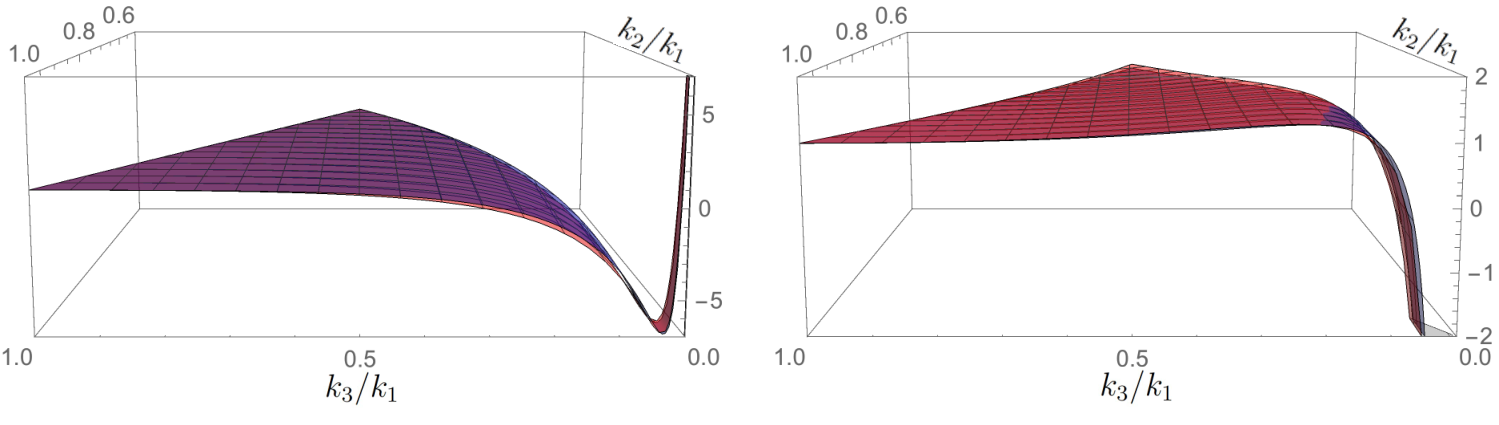
For single-isocurvaton QSFI with , the shape function has been approximated as Chen:2009zp:
| (34) |
A good phenomenological fit to the multi-isocurvaton QSFI shape is
| (35) |
where the normalization enforces in the equilateral limit. Note that the shape function is parameterized by three numbers , , and a phase . In Fig. 3, we plot the shape functions evaluated numerically against the shape functions computed with (35).
We can also define the parameter , corresponding to the magnitude of this shape. In keeping with convention99 9 Conventionally, is defined via where is given by the power spectrum’s normalization (see, e.g. Ade:2015xua)., we define:
| (36) |
By matching the squeezed limit of (36) onto (28), we can obtain as a function of :
| (37) |
Even for , the oscillating QSFI bispectrum shape still displays qualitatively distinct features. Specifically, the shape can get large and negative in the squeezed limit. This is different from many other bispectrum shapes that grow in the squeezed limit because they typically remain positive rather than become negative (see Ade:2015ava).
III.2 Collapsed Trispectrum

We now consider the four-point function of , which is defined as
| (38) |
We focus on the collapsed limit, which occurs when , , and . The integrand will be symmetric in and , which means we can untangle the limits of the time integrals. The collapsed four-point then simplifies to
| (39) | ||||
| (40) | ||||
| (41) | ||||
| (42) |
Note, not every term oscillates logarithmically in . Instead, there are two terms which oscillate with angular frequency as well as one that does not oscillate at all in .
It turns out that a loop contribution to the trispectrum can produce terms that oscillate with frequency . We explore this in Appendix B.
IV Large-Scale Structure
In this section, we determine the effects of PNG on large-scale structure, specifically the halo-halo power spectrum and the matter-halo power spectrum . It is well known that in certain inflationary theories, such as single-isocurvaton QSFI, the contributions of PNG to and can become much larger than the Gaussian contributions at wavevectors of order An:2017rwo; McAneny:2017bbv; An:2018tcq. We now consider this in multi-isocurvaton QSFI.
The primordial curvature perturbations are related to the linearly evolved smoothed matter density perturbations today, , by Dodelson book
| (43) |
where is the ratio of the matter density and the critical density today, is the Hubble constant today, is the BBKS transfer function Bardeen:1985tr and is a window function smoothing over radius . We use the top-hat window function
| (44) |
.
Since we are interested in scales of order Mpc/, can be related to through a bias expansion. For simplicity, we use a local-in-matter-density bias expansion (for a more comprehensive treatment, see Desjacques:2016bnm)
| (45) |
The bias coefficients can be approximated using the threshold model introduced in Kaiser:1984sw. We assume that halos form instantaneously at some redshift , and that halos only form at points where the overdensity exceeds some critical threshold . We also neglect the evolution of halos after collapse. In this model, the bias coefficients and are then
| (46) |
where . In deriving our numerical results, we use , which corresponds to at Press:1973iz, and . While a more sophisticated treatment of halo dynamics will change our precise numerical results, we do not expect them to impact our conclusions qualitatively.
We will be interested in computing the halo-halo power spectrum ,
| (47) |
as well as the halo-matter power spectrum ,
| (48) |
The Gaussian contributions to and are found to be
| (49) | ||||
| (50) |
At wavevectors of order , the most significant non-Gaussian contributions to are due to the squeezed and collapsed limits of the bispectrum (28) and trispectrum (39). Then, plugging (43) and (45) into (47) and using (28) and (39) gives
| (51) | ||||
| (52) | ||||
| (53) | ||||
| (54) | ||||
| (55) | ||||
| (56) | ||||
| (57) |
where, to compactify notation, we have defined
| (58) |
The most significant non-Gaussian contribution to comes from the squeezed bispectrum:
| (59) | ||||
| (60) | ||||
| (61) |

In Figure 5 we plot (51) for the model parameters (19) and (21) and . Note that at around , begins to deviate from . The oscillations evident in Fig. 5 are a consequence of the oscillatory squeezed bispectrum and collapsed trispectrum.
However, for , the amplitude of the oscillations is quite small. Moreover, the non-Gaussian contributions to only begin to dominate over the Gaussian contribution at a scale of order , which is unlikely to be detected experimentally in the near future.
This scale is smaller than the scale at which the non-Gaussian contributions to begin to dominate in single-isocurvaton QSFI theories with and small An:2017rwo. The reason is the integrals involving the transfer functions, , are oscillatory in multi-isocurvaton QSFI when , which washes them out. This makes the coefficients of the non-Gaussian contributions smaller in multi-isocurvaton QSFI than in single-isocurvaton QSFI.
V Conclusion
In this paper, we studied quasi-single field inflation with multiple isocurvatons. Multi-isocurvaton QSFI includes the interaction which can give rise to novel inflationary dynamics. In particular, the mode functions of and can exhibit late time log oscillations that decay slowly as . Due to these late time oscillations, the primordial non-Gaussianities of exhibit log-oscillatory behavior in ratios of wavevector magnitudes.
For example, the bispectrum is proportional to in the squeezed limit, which means for small it experiences nearly cubic growth while oscillating. This behavior cannot be achieved in single-isocurvaton QSFI. Furthermore, the collapsed trispectrum goes as , i.e. there is a term that does not oscillate in as well as one that does with frequency .
In models where , the contributions of the squeezed bispectrum and collapsed trispectrum to the halo-halo power spectrum and the halo-matter power spectrum can dominate over the Gaussian contributions at . When , and oscillate logarithmically in .
ACKNOWLEDGEMENTS
We would like to thank Mark Wise for useful discussions. This work was supported by the DOE Grant DE-SC0011632. We are also grateful for the support provided by the Walter Burke Institute for Theoretical Physics.
Appendix A Commutator Constraints
The integrals of (31) are potentially IR divergent because of the factors of in the integrands. It can be shown that all potentially IR divergent terms are zero. Eq. (11) implies that the mode functions can be written in series form as
| (62) | ||||
| (63) |
The equal time commutation relation holds order by order in powers of and implies the following relations among the power series coefficients
| (64) |
where the sum over mode label is implicit. Furthermore, the mode equations (11) imply
| (65) |
Combining the first relation in (A) with (65) yields
| (66) |
The leading infrared behavior of (31) is then
| (67) |
It is straightforward to fit the mode functions to (62) and determine the numerical coefficient in (67). The method to evaluate is to choose an and numerically integrate from using (31) and then integrate from using (67).
Appendix B Loop Contribution to the Collapsed Trispectrum
Recall that the tree-level collapsed trispectrum, which has one internal line, has terms that oscillate with frequency . We now show that a loop contribution to the collapsed trispectrum, which has two internal lines, can contain terms that oscillate with frequency . The loop contribution to the collapsed trispectrum then induces terms in the halo-halo power spectrum that oscillate as .1010 10 Contributions to the halo-halo power spectrum due to primordial non-Gaussianities sourced by quantum loops in the context of single-isocurvaton QSFI were considered in McAneny:2017bbv; An:2018tcq.

Consider a theory in which the interaction Hamiltonian is composed of a single interaction:
| (68) |
Inserting two factors of (68) into (23) yields the 1-loop contribution to the trispectrum:
| (69) |
As described in Arkani-Hamed:2015bza; McAneny:2017bbv; An:2018tcq, for , the loop diagram can give a large contribution to the collapsed trispectrum. In this limit, the loop integral is dominated by the region in which , which means the mode functions on the bottom line of (B) can be expanded in . Defining the integral
| (70) |
where is an arbitrary unit vector, the loop contribution can be written:
| (71) | ||||
| (72) | ||||
| (73) | ||||
| (74) |
where
| (75) | ||||
| (76) | ||||
| (77) | ||||
| (78) |
Note that the loop contribution to the trispectrum has terms that do not oscillate with , terms that oscillate with frequency , and terms that oscillate with frequency .
The loop contribution to due to the quartic interaction can also be computed:
| (79) | ||||
| (80) | ||||
| (81) | ||||
| (82) | ||||
| (83) | ||||
| (84) |
While it appears that the terms oscillating with frequency in (79) could induce unique observable features in , it turns out their coefficients are suppressed relative to those of the non-oscillating terms since . This can be understood by noting that while the magnitudes of the integrands of and are the same, the integrand of is oscillatory and washes out.
References
- (1) A. A. Starobinsky, JETP Lett. 30, 682 (1979); Phys. Lett. B. 91, 99 (1980); A. Guth, Phys. Rev. D23, 347 (1981); A. D. Linde, Phys. Lett. B 108, 389 (1982); 114, 431 (1982); A. Albrecht and P. Steinhardt, Phys. Rev. Lett. 48, 1220 (1982).
- (2) S. V. Mukanov and G. V. Chibisov, Sov. Phys. JETP Lett. 33, 532 (1981); S. Hawking, Phys. Lett. B115, 295 (1982); A. A. Starobinsky, Phys. Lett. B 117, 175 (1982); A. Guth and S.-Y. Pi, Phys. Rev. Lett 49, 1110 (1982); J. M. Bardeen, P. Steinhardt and M. S. Turner, Phys. Rev. D28, 679 (1983).
- (3) D. Baumann, doi:10.1142/9789814327183-0010 arXiv:0907.5424 [hep-th].
- (4) C. Cheung, P. Creminelli, A. L. Fitzpatrick, J. Kaplan and L. Senatore, JHEP 0803, 014 (2008) doi:10.1088/1126-6708/2008/03/014 [arXiv:0709.0293 [hep-th]].
- (5) J. M. Maldacena, JHEP 0305, 013 (2003) doi:10.1088/1126-6708/2003/05/013 [astro-ph/0210603].
- (6) M. Alishahiha, E. Silverstein and D. Tong, Phys. Rev. D 70, 123505 (2004) doi:10.1103/PhysRevD.70.123505 [hep-th/0404084].
- (7) X. Chen, R. Easther and E. A. Lim, JCAP 0706, 023 (2007) doi:10.1088/1475-7516/2007/06/023 [astro-ph/0611645].
- (8) X. Chen and Y. Wang, JCAP 1004, 027 (2010) doi:10.1088/1475-7516/2010/04/027 [arXiv:0911.3380 [hep-th]].
- (9) X. Chen, Adv. Astron. 2010, 638979 (2010) doi:10.1155/2010/638979 [arXiv:1002.1416 [astro-ph.CO]].
- (10) D. Baumann and D. Green, JCAP 1109, 014 (2011) doi:10.1088/1475-7516/2011/09/014 [arXiv:1102.5343 [hep-th]].
- (11) D. Baumann and D. Green, Phys. Rev. D 85, 103520 (2012) doi:10.1103/PhysRevD.85.103520 [arXiv:1109.0292 [hep-th]].
- (12) V. Assassi, D. Baumann and D. Green, JCAP 1211, 047 (2012) doi:10.1088/1475-7516/2012/11/047 [arXiv:1204.4207 [hep-th]].
- (13) T. Noumi, M. Yamaguchi and D. Yokoyama, JHEP 1306, 051 (2013) doi:10.1007/JHEP06(2013)051 [arXiv:1211.1624 [hep-th]].
- (14) H. An, M. McAneny, A. K. Ridgway and M. B. Wise, JHEP 1806, 105 (2018) doi:10.1007/JHEP06(2018)105 [arXiv:1706.09971 [hep-ph]].
- (15) H. An, M. McAneny, A. K. Ridgway and M. B. Wise, Phys. Rev. D 97, no. 12, 123528 (2018) doi:10.1103/PhysRevD.97.123528 [arXiv:1711.02667 [hep-ph]].
- (16) X. Chen, M. x. Huang, S. Kachru and G. Shiu, JCAP 0701, 002 (2007) doi:10.1088/1475-7516/2007/01/002 [hep-th/0605045].
- (17) X. Chen, JCAP 1012, 003 (2010) doi:10.1088/1475-7516/2010/12/003 [arXiv:1008.2485 [hep-th]].
- (18) I. Agullo and L. Parker, Gen. Rel. Grav. 43, 2541 (2011) [Int. J. Mod. Phys. D 20, 2861 (2011)] doi:10.1007/s10714-011-1220-8, 10.1142/S0218271811020731 [arXiv:1106.4240 [astro-ph.CO]].
- (19) I. Agullo and L. Parker, Phys. Rev. D 83, 063526 (2011) doi:10.1103/PhysRevD.83.063526 [arXiv:1010.5766 [astro-ph.CO]].
- (20) P. Adshead, C. Dvorkin, W. Hu and E. A. Lim, Phys. Rev. D 85, 023531 (2012) doi:10.1103/PhysRevD.85.023531 [arXiv:1110.3050 [astro-ph.CO]].
- (21) A. Achucarro, J. O. Gong, G. A. Palma and S. P. Patil, Phys. Rev. D 87, no. 12, 121301 (2013) doi:10.1103/PhysRevD.87.121301 [arXiv:1211.5619 [astro-ph.CO]].
- (22) A. Achucarro, V. Atal, B. Hu, P. Ortiz and J. Torrado, Phys. Rev. D 90, no. 2, 023511 (2014) doi:10.1103/PhysRevD.90.023511 [arXiv:1404.7522 [astro-ph.CO]].
- (23) S. R. Behbahani, A. Dymarsky, M. Mirbabayi and L. Senatore, JCAP 1212, 036 (2012) doi:10.1088/1475-7516/2012/12/036 [arXiv:1111.3373 [hep-th]].
- (24) N. Arkani-Hamed and J. Maldacena, arXiv:1503.08043 [hep-th].
- (25) R. Flauger, L. McAllister, E. Silverstein and A. Westphal, JCAP 1710, no. 10, 055 (2017) doi:10.1088/1475-7516/2017/10/055 [arXiv:1412.1814 [hep-th]].
- (26) R. Flauger, M. Mirbabayi, L. Senatore and E. Silverstein, JCAP 1710, no. 10, 058 (2017) doi:10.1088/1475-7516/2017/10/058 [arXiv:1606.00513 [hep-th]].
- (27) Y. Wang, Y. P. Wu, J. Yokoyama and S. Zhou, JCAP 1807, no. 07, 068 (2018) doi:10.1088/1475-7516/2018/07/068 [arXiv:1804.07541 [astro-ph.CO]].
- (28) N. Bolis, A. Albrecht and R. Holman, arXiv:1902.07567 [hep-th].
- (29) P. A. R. Ade et al. [Planck Collaboration], Astron. Astrophys. 594, A17 (2016) doi:10.1051/0004-6361/201525836 [arXiv:1502.01592 [astro-ph.CO]].
- (30) T. J. Allen, B. Grinstein and M. B. Wise, Phys. Lett. B 197, 66 (1987). doi:10.1016/0370-2693(87)90343-1
- (31) N. Dalal, O. Dore, D. Huterer and A. Shirokov, Phys. Rev. D 77, 123514 (2008) doi:10.1103/PhysRevD.77.123514 [arXiv:0710.4560 [astro-ph]].
- (32) D. Baumann, S. Ferraro, D. Green and K. M. Smith, JCAP 1305, 001 (2013) doi:10.1088/1475-7516/2013/05/001 [arXiv:1209.2173 [astro-ph.CO]].
- (33) J. Gleyzes, R. de Putter, D. Green and O. Doré, JCAP 1704, no. 04, 002 (2017) doi:10.1088/1475-7516/2017/04/002 [arXiv:1612.06366 [astro-ph.CO]].
- (34) N. Aghanim et al. [Planck Collaboration], arXiv:1807.06209 [astro-ph.CO].
- (35) R. Gwyn, G. A. Palma, M. Sakellariadou and S. Sypsas, JCAP 1304, 004 (2013) doi:10.1088/1475-7516/2013/04/004 [arXiv:1210.3020 [hep-th]].
- (36) V. Assassi, D. Baumann, D. Green and L. McAllister, JCAP 1401, 033 (2014) doi:10.1088/1475-7516/2014/01/033 [arXiv:1304.5226 [hep-th]].
- (37) S. Weinberg, Phys. Rev. D 72, 043514 (2005) doi:10.1103/PhysRevD.72.043514 [hep-th/0506236].
- (38) P. A. R. Ade et al. [Planck Collaboration], Astron. Astrophys. 594, A13 (2016) doi:10.1051/0004-6361/201525830 [arXiv:1502.01589 [astro-ph.CO]].
- (39) M. McAneny, A. K. Ridgway, M. P. Solon and M. B. Wise, Phys. Lett. B 785, 332 (2018) doi:10.1016/j.physletb.2018.06.026 [arXiv:1712.07657 [astro-ph.CO]].
- (40) H. An, M. B. Wise and Z. Zhang, arXiv:1806.05194 [hep-ph].
- (41) S. Dodelson, “Modern Cosmology,” Amsterdam, Netherlands: Academic Pr. (2003) 440 p
- (42) J. M. Bardeen, J. R. Bond, N. Kaiser and A. S. Szalay, Astrophys. J. 304 (1986) 15. doi:10.1086/164143
- (43) V. Desjacques, D. Jeong and F. Schmidt, Phys. Rept. 733, 1 (2018) doi:10.1016/j.physrep.2017.12.002 [arXiv:1611.09787 [astro-ph.CO]].
- (44) N. Kaiser, Astrophys. J. 284, L9 (1984). doi:10.1086/184341
- (45) W. H. Press and P. Schechter, Astrophys. J. 187, 425 (1974). doi:10.1086/152650