Vainshtein regime in Scalar-Tensor gravity: constraints on DHOST theories
Abstract
We study the screening mechanism in the most general scalar-tensor theories that leave gravitational waves unaffected and are thus compatible with recent LIGO/Virgo observations. Using the effective field theory of dark energy approach, we consider the general action for perturbations beyond linear order, focussing on the quasi-static limit. When restricting to the subclass of theories that satisfy the gravitational wave constraints, the fully nonlinear effective Lagrangian contains only three independent parameters. One of these, , is uniquely present in degenerate higher-order theories. We compute the two gravitational potentials for a spherically symmetric matter source and we find that for they decrease as the inverse of the distance, as in standard gravity, while the case is ruled out. For , the two potentials differ and their gravitational constants are not the same on the inside and outside of the body. Generically, the bound on anomalous light bending in the Solar-System constrains . Standard gravity can be recovered outside the body by tuning the parameters of the model, in which case from the Hulse-Taylor pulsar. Theories conformally related to General Relativity admit , at least for a specific choice of conformal couplings.
I Introduction
Scalar-tensor theories are currently used to extend gravity beyond General Relativity on cosmological scales. The higher-derivate terms that characterize Horndeski Horndeski:1974wa; Deffayet:2011gz and beyond-Horndeski theories Zumalacarregui:2013pma; Gleyzes:2014dya; Langlois:2015cwa; Crisostomi:2016czh; BenAchour:2016fzp (see also Langlois:2018dxi; Kobayashi:2019hrl for recent reviews), while possibly providing an origin for the observed accelerated expansion of the Universe, are crucial to suppress modifications of gravity on Solar-System, where very stringent tests apply Will:2014xja.
Indeed, close to matter sources, the nonlinearities of the scalar field suppress its effects through the so-called Vainshtein screening mechanism Vainshtein:1972sx; Babichev:2013usa, allowing General Relativity to be recovered. Screening is essential for the theories under consideration to be observationally viable.
However, recent observations of gravitational waves have put severe constraints on higher-derivative operators. The simultaneous observation of gravitational waves and gamma ray bursts from the GW170817 event has constrained very precisely the relative speed between gravitons and photons TheLIGOScientific:2017qsa, eliminating part of the derivative couplings of the scalar field to the curvature Creminelli:2017sry; Sakstein:2017xjx; Ezquiaga:2017ekz; Baker:2017hug.11 1 As discussed in deRham:2018red, this conclusion can be evaded if new physics appears at a scale parametrically smaller than the observed LIGO/Virgo frequencies.More recently, it has been pointed out that the theories beyond Horndeski belonging to the Gleyzes-Langlois-Piazza-Vernizzi (GLPV) class Gleyzes:2014dya; Gleyzes:2014qga display a cubic graviton-scalar-scalar interaction that can mediate an observable decay of the graviton into dark energy particles Creminelli:2018xsv. The same vertex is responsible for an anomalous gravitational wave dispersion, when the speeds of scalar and gravitational wave differ. These two effects may become important at frequencies relevant for LIGO/Virgo observations, leading to a very tight constraint on these theories.22 2 Recently, positivity bounds for scalar theories coupled to gravity Bellazzini:2019xts have decreased significantly the regime of validity of the corresponding EFTs (e.g. for the cubic galileon Nicolis:2008in). It would be interesting to study how these theoretical constraints affect general theories with screening.
In this article we study the subclass of scalar-tensor theories that leave gravitational waves unaffected and satisfy these constraints exactly. This study is the natural continuation of Ref. Kobayashi:2014ida, which examined the Vainshtein mechanism in GLPV theories, and of Refs. Crisostomi:2017lbg; Langlois:2017dyl; Dima:2017pwp, where this investigation was extended to Degenerate Higher-Order Scalar-Tensor (DHOST) theories Langlois:2015cwa; Crisostomi:2016czh; BenAchour:2016fzp, in the case where the speed of gravitational waves equals the one of light. These references showed that for the subclass of these theories extending Horndeski, the two gravitational potentials differ inside matter and depend on the density profile, signalling the breaking of the Vainshtein screening. (See for instance also Bartolo:2017ibw; Ganz:2018vzg; Babichev:2018rfj; Kase:2018iwp; Crisostomi:2017pjs; Crisostomi:2018bsp; Frusciante:2018tvu for other studies on the surviving theories and Kase:2018aps; Ezquiaga:2018btd for reviews.)
As in these references, here we consider the solutions for the gravitational potentials in these theories near matter sources, i.e. in the Vainshtein regime, and compare them to observational data. We will rely on the quasi-static approximation, which is valid on scales much smaller than the Hubble radius when we restrict to non-relativistic sources.
In the next section we review DHOST theories and their effective description, and we expand the action in the metric potentials and scalar field perturbations. We then discuss the subset of theories that evade the gravitational wave constraints. We briefly study the linear theory in Sec. III and the Vainshtein regime around a spherically symmetric source in Sec. IV. Here, we also discuss our results in the more familiar Horndeski frame. The previous discussions do not apply to theories that are related to General Relativity by a conformal transformation, which are the subject of Sec. V. Finally, constraints on the parameters are derived in Sec. VI, and conclusions are left to Sec. VII.
II Action and perturbation equations
II.1 DHOST theories
We denote by the semicolon a covariant derivative and we define . The action for DHOST theories includes all possible quadratic combinations up to second derivatives of the field and reads Langlois:2015cwa
| (1) | ||||
where is the 4D Ricci scalar and the are defined by
| (2) |
The functions and do not affect the degeneracy character of the theory. Instead, for DHOST theories, the functions appearing in the second line of eq. (1) must satisfy three degeneracy conditions Langlois:2015cwa that fix three of these functions in terms of the others. Here we are going to focus on the subclass that satisfy (and two other degeneracy conditions). Other subclasses have been shown to display a linear instability, either in the scalar or in the tensor sector deRham:2016wji; Langlois:2017mxy.
II.2 Effective description and constraints
It is convenient to discuss observational constraints on these theories in terms of the EFT of dark energy parameters, which for DHOST theories have been introduced in Langlois:2017mxy and extended to nonlinear order in the perturbations in Dima:2017pwp.
Specifically, in the presence of a preferred slicing induced by a time-dependent scalar field, we can choose the time as to coincide with the uniform field hypersurfaces. In this gauge, called the unitary gauge, and using the ADM metric decomposition with line element , cosmological perturbations around an FRW solution are governed by the action
| (3) |
where we have written only the operators with the highest number of spatial derivatives, which are relevant in the quasi-static limit. Here (a dot denotes the time derivative), , is the perturbation of the extrinsic curvature of the time hypersurfaces, its trace, and is the 3D Ricci scalar of these hypersurfaces. Moreover, , and .
The time-dependent functions in this action are related to the free functions in eq. (1). One finds that the effective Planck mass that normalizes the graviton kinetic energy is given by . The other parameters read Dima:2017pwp
| (4) |
The function Bellini:2014fua measures the kinetic mixing between metric and scalar fluctuations Creminelli:2008wc and the fractional difference between the speed of gravitons and photons. The function measures the kinetic mixing between matter and the scalar fluctuations Gleyzes:2014dya; Gleyzes:2014qga; DAmico:2016ntq and vanishes for Horndeski theories, while the function parameterizes the only operator that starts cubic in the perturbations Cusin:2017mzw.
Finally, the functions , , and parameterize the presence of higher-order operators. The degeneracy conditions, which we assume hereafter, read Langlois:2017mxy
| (5) |
so that only is independent. Another function that we define here for later convenience is Bellini:2014fua
| (6) |
II.3 Action in Newtonian gauge
To study scalar linear and higher-order perturbations we will exit the unitary gauge and work in the Newtonian gauge, where the metric is written as
| (7) |
The scalar field is introduced by performing a space-time dependent shift in the time . Then, we expand the action eq. (3) in terms of the metric and scalar field perturbations. We keep only terms with the highest number of derivatives per field, which are those relevant in the quasi-static limit, and we find
| (8) |
with
| (9) | ||||
where we have defined for , and , and are time-dependent coefficients, reported in App. A.1.
The last term in the bracket is the matter Lagrangian. If we define by the matter energy density and by its mean cosmological value, this is given by
| (10) |
where .
The field equations can be derived straightforwardly by varying the action eq. (8) with respect to , and . We have
| (11) |
where the explicit expressions of can be found in App. A.1 (see eqs. (70)–(72)).
The above Lagrangians and equations are valid for general DHOST theories. We will now consider the subclass of theories leaving the gravitational wave unaffected.
II.4 Gravitational wave constraints
We now focus on the subset of theories that evade the gravitational wave constraints. In particualr, we demand that gravity and light travel at the same speed, i.e. (see e.g. Creminelli:2017sry),
| (12) |
Moreover, we require that gravitons do not decay into dark energy by setting Creminelli:2018xsv
| (13) |
Unless otherwise stated, in the following we impose these two equations and replace and in terms of .
In terms of the functions in the action eq. (1), these requirements, together with the degeneracy conditions, read and , for any , i.e., Creminelli:2018xsv ,
| (14) |
From eq. (4), in this subset of theories the remaing free parameters are thus given by
| (15) |
III Linear regime
We briefly discuss how matter inhomogeneities source and the gravitational potentials at linear order. For convenience, we first define the combination
| (16) |
where is the effective sound speed of dark energy fluctuations Langlois:2017mxy, which must be positive to avoid gradient instabilities, while the time-dependent function is the coefficient in front of the time kinetic term of scalar fluctuations (see Langlois:2017mxy), which must be positive to avoid ghosts. In practice, we do not need their explicit expressions because in the quasi-static limit these two parameters always appear in the combination .
By solving for and the linear equations obtained by varying the action with respect to the two metric potentials, and replacing these solutions in the scalar field equation, we obtain
| (17) |
where is the value of the Planck mass measured today and the parameters , and above are defined as
| (18) |
This choice of definitions will become clearer when we consider the full nonlinear equation for , in Sec. IV.
For completeness, we also provide the solutions for the metric potentials, which can be obtained by replacing eq. (17) back into the equations for and . One finds Crisostomi:2017pjs; Hirano:2019nkz
| (19) | ||||
where the coefficients on the right-hand side are given in App. A.2. Observational constraints on the above coefficients of the linear equations are discussed in Hirano:2019nkz. We are now ready to discuss the Vainshtein regime.
IV Vainshtein regime
In this section we want to study the Vainshtein mechanism around a spherically symmetric body, such as for instance a non-relativistic star (see Kobayashi:2018xvr for a study of relativistic stars in DHOST theories). This is at play close to the body, where non-linearities of the scalar field become important suppressing the scalar force. Far from the body, the linear solutions affected by the fifth force (see eq. (19)) are recovered. This can allow the theory to be compatible with stringent Solar System observations while at the same time modifying gravity on large scales.
To derive the equations relevant for spherically symmetric solutions, we assume that all of the fields depend only on time and the radial variable, , where . Then, we integrate the field equations eq. (11) over the radial variable and use Stoke’s theorem. Following Kobayashi:2014ida, we use the following notation,
| (20) |
where a prime denotes a derivative with respect to and is a mass scale of order , where is the Hubble rate today. Moreover, we define
| (21) |
where is the physical mass of an overdensity contained in a spherical ball of physical radius . The quantity represents the comoving mass density contrast in this ball.
The explicit expressions of the field equations in spherical symmetry are reported in App. A.3. Following Crisostomi:2017lbg; Langlois:2017dyl; Dima:2017pwp, we can solve the first two equations for and and plug the solutions into the third equation. After imposing the degeneracy conditions eq. (5), one obtains a polynomial equation for only. This equation was previously studied after imposing that gravitons and photons propagate with the same speed, eq. (12), in Crisostomi:2017lbg; Langlois:2017dyl and in the general case in Dima:2017pwp and a cubic equation was obtained. Here we further restrict to theories where the gravitational waves do not decay, i.e. eq. (13). In this case one finds instead a quadratic equation,
| (22) |
where the time-dependent functions , and already appeared in the linear equations and are defined in eq. (18). The other functions are given by
| (23) |
with
| (24) |
If , the term proportional to becomes important close to the matter source, while it is negligible far away from it. The transition happens at the so-called Vainshtein radius, roughly corresponding to , i.e.,
| (25) |
For example, for a star like the sun, the Vainshtein radius is about a tenth of the size of the Milky Way.
For , the term quadratic in vanishes and the usual Vainshtein screening cannot be supported. As shown in Sec. IV.3, this case corresponds to scalar-tensor theories that are conformally related to General Relativity, i.e., that can be described by the Einstein-Hilbert term plus conformally coupled matter. Here we will assume that (and thus ) does not vanish. We discuss the case in Sec. V.
As discussed in Sec. III, . Thus, for , defined in eq. (18) is also positive and the solution to eq. (22) that matches the linear regime, i.e., that has the correct behavior for , is
| (26) | ||||
where for convenience we have defined the positive function,
| (27) |
The terms proportional to and in eq. (22) contain respectively the radial and time derivative of the comoving mass of the body. Thus, when the mass of the central overdensity is constant in time and space, such as at a radial distance larger than the body size, we have and . Therefore, we consider two different cases, depending on whether we are outside or inside the object.
IV.1 Inside of matter
Inside of matter, is generally different from zero, in which case, when , the term proportional to can dominate the square root in eq. (26). This regime is characterized by
| (28) |
and
| (29) |
where on the right-hand side we have used the definitions in eq. (18) and eq. (23) and that . The right-hand sides of these equalities are of order unity while, on the left-hand side, . For instance, inside a star like the sun,33 3 Here and in the rest of this paper, we use the symbol to denote the appropriate quantity for our sun.
| (30) |
where we have used . These conditions are thus realized inside matter unless becomes . Using a mass profile from the Lane-Emden equation (see eq. (83) in the appendix), we have verified that this happens only on a very thin region near the surface of the star.
Now, expanding the solution in eq. (26) for and , we can distinguish between two cases. When , the solution for is given by
| (31) |
This solution can then be plugged back into the field equations for and (see eqs. (77) and (78)) to solve for these two variables. Since , the equations for and are dominated by the usual matter term linear in and terms both linear and quadratic in can be neglected.
The solutions for the potentials can be straightforwardly computed and read
| (32) |
where is the gravitational constant that canonically normalizes the graviton, and
| (33) |
Thus, in this theory so that Vainshtein screening is broken inside the body. Notice that the breaking is different from the one found in Kobayashi:2014ida; Crisostomi:2017lbg; Langlois:2017dyl; Dima:2017pwp, which depends on the radial derivatives of the object mass.
The case is instead ruled out. Indeed, in this case the solution eq. (26) reads
| (34) |
Therefore, is not suppressed inside matter and nonlinear terms proportional to dominate the field equations for and . The solutions,
| (35) |
are incompatible with the existence of stars or other bounded objects.
IV.2 Outside of matter
Using eq. (21) outside the object, where the physical mass is constant, we have and . Replacing this in eq. (26), near the source we obtain
| (36) |
In contrast with the solution inside matter, eq. (31), where , here so that terms quadratic in contribute to the and solutions while linear terms are negligible.
The solutions for the potentials become now
| (37) |
with
| (38) | ||||
where for convenience we have defined a new quantity,
| (39) |
From these expressions, it is clear that the Vainshtein mechanism is broken also outside of the matter source because the two gravitational potentials are different. Only for
| (40) |
are the two potentials the same and the Vainshtein screening recovered outside of matter.
An example of the solutions eq. (32) (for ) and eq. (37) (for ) is presented in Fig. 1. Notice the suppressed value of . For a large overdensity , such as in a star, the transition between the interior of the star, where eqs. (28) and (29) are satisfied, and the exterior, where , takes place abruptly, so that , and visually display a discontinuity for . Of course, the solutions are actually continuous, as follows for instance from eq. (26).

IV.3 The Horndeski frame
The above results can be understood by noticing that DHOST theories that we consider in this paper can be mapped to Horndeski theories via an invertible -dependent conformal and disformal transformation Crisostomi:2016czh; Achour:2016rkg.
Since we want to preserve the speed of propagation of gravitons, we focus on conformal transformations only, i.e.
| (41) |
and use the tilde to denote quantities in the Horndeski frame. For convenience, we also introduce the dimensionless time-dependent parameter
| (42) |
with the right-hand side of this equation evaluated on the background solution.
The relations to compute the transformation of the EFT parameters of the action eq. (3) under the change of frame eq. (41) are given in Langlois:2017mxy (see for instance eq. (2.22) of that reference). Without loss of generality, we will assume that on the background solution, so that and . Moreover, for the transformation above, one finds
| (43) |
while .
Using these relations, one can show that a DHOST theory with gravitational metric satisfying the conditions eq. (12) and eq. (13) (see its covariant form in eq. (14)), is equivalent to a Horndeski theory with gravitational metric ,44 4 Since matter is coupled to , the coupling to matter in the new frame is non-minimal; see below. with and and action
| (44) |
provided that . Additionally, we obtain Langlois:2017mxy (see eq. (C.14) of that reference)
| (45) |
Using the above transformations we can check that given in eq. (24) can be written in terms of Horndeski-frame quantities as . As mentioned below eq. (24), this vanishes for , i.e. for Brans-Dicke Brans:1961sx, Carroll:2004de or other theories conformally related to General Relativity Gleyzes:2015pma.
In the Horndeski frame, the EFT action eq. (8) is given by
| (46) |
Here the Lagrangians , and have analogous expressions as those in eq. (9), but now fields and parameters are tilded and .
Using eq. (41) and focusing on the leading order in spatial derivatives to retain only terms relevant in the quasi-static limit, the potentials in the Horndeski frame are related to those in the DHOST frame by
| (47) | ||||
while it is straigforward to verify that the scalar field fluctuation does not change,
| (48) |
While the metric transforms when changing frame, matter remains always minimally coupled to the gravitational metric in the DHOST frame, i.e. . Therefore, . Using eq. (10) and the relations above, the coupling in the Horndeski frame is thus
| (49) |
We can now vary the action eq. (46) with respect to , and . Actually, using the above functional relationships between the Horndeski action and the DHOST action , we can easily derive the relationship between the Horndeski frame equations of motion, and the DHOST frame equations of motion eq. (11) using the chain rule,
| (50) |
This gives
| (51) | ||||
Using the field equations , we can solve the system assuming spherical symmetry around a body, similarly to what was done earlier in Sec. IV. The equations for and read
| (52) |
(i.e. all nonlinear terms vanish), and the closed equation for remains the same as that of , eq. (22), as expected. Since terms linear in can be neglected both inside and outside of matter, the solutions to the above equations become, in terms of the potentials in the Horndeski frame,
| (53) |
both inside and outside of the source, as long as .
With eq. (53), we can now verify what we found in the previous subsections. Inside matter, can be neglected in eq. (47) and eq. (32) is recovered. Outside matter, can be neglected but cannot. Replacing in eq. (47) the solution for , eq. (36), we can recover the solution outside the body, eq. (37).
Moreover, the conformal transformation eq. (47) leaves the sum of the potentials invariant. One can verify directly that our expressions inside eq. (32) and outside eq. (37) of the source satisfy , where we have used eq. (53) for the last equality. Additionally, the fact that the solutions in the Horndeski frame eq. (53) are valid both inside or outside of the source means that , which can be verified directly in eq. (38).
V Theories conformally related to General Relativity
In the previous section we focused on theories with . Here we consider the case , which corresponds to theories related to General Relativity by the conformal transformation (41), as shown in Sec. IV.3. Their general action is given by eq. (14) with . Examples are Jordan-Brans-Dicke Brans:1961sx and theories Carroll:2004de, but here we are interested in extentions of these theories where the conformal factor relating them to General Relativity depends also on , in which case .
When , the equation for , eq. (22), becomes linear. Inside of matter, the term proportional to dominates the solution so that one obtains the same conclusions as in Sec. IV.1 (including the constraint ).
Thus, we focus on the solutions outside of matter and near the source. In that case, the solution for is simply the linear solution,
| (54) |
Solving the equations for and with this solution we have, in terms of and ,
| (55) |
This is clearly incompatible with Solar System tests unless is practically zero.
A possible way out with is to consider the subclass of theories with . Taking into account that , this fixes all parameters as a function of , i.e.,
| (56) |
For this particular case the source term in eq. (22) is absent and the fifth force vanishes, . Thus, the gravitational potentials outside the source are linear in the object mass and coincide with the solutions eq. (32), which were obtained ignoring the scalar field contribution.
VI Constraints
Let us discuss observational constraints on the parameters of the theories studied above, in particular on . A first class of constraints comes from stellar physics. We have studied them in App. B and have shown that they lead to complementary (but weaker) constraints to those derived in the following.
As shown in Jimenez:2015bwa, for the decrease of the orbital period of binary stars is proportional to the ratio between the gravitational constant normalizing the gravitons, , and the one entering the Kepler law, which here is taken to be the one outside the object, . Thus, using the results from Weisberg:2010zz, the Hulse-Taylor pulsar (PSR B1913+16) Hulse:1974eb allows us to constrain ,
| (57) |
Next, we move to the Cassini constraints. Measurements of the frequency shift of radio waves, sent to and from the Cassini spacecraft as they passed near the sun Bertotti:2003rm, constrain the post-Newtonian parameter to be . Since eq. (57) says that is small, we can approximate and use this measurement to constrain the relative difference between the gravitational potentials outside of matter,
| (58) |
Using eq. (37) we can rewrite the above quantity as
| (59) |
where we remind the reader that and are respectively defined in eqs. (24) and (39). For generic values of , and , one expects that , so that the above turns into a tight constraint on ,
| (60) |
The bound on the left-hand side comes from the result of Sec. IV.1 that negative values of are not allowed.
A more conservative constraint on , independent of , , and , comes from isolating by using eq. (38). One obtains
| (61) |
Combined with the constraint , this gives
| (62) |
which also holds in the presence of the tuning .
The previous discussion assumed . Theories that are conformally related to General Relativity have . As discussed in Sec. V, these theories are ruled out unless they satisfy the condition (56). In this case, the post-Newtonian parameter reads
| (63) |
Combining with the Cassini constraint, eq. (58), gives
| (64) |
VII Conclusion
Vainshtein screening is crucial to pass the stringent tests of gravity available at local scales. We studied the Vainshtein regime in the most general subset of DHOST theories that evade all of the constraints from gravitational wave observations, i.e., for which gravitons propagate at the speed of light and do not decay.
For non-zero values of the parameter that characterizes the higher-order derivatives in DHOST theories, i.e. , the screening mechanism is broken. Negative values of are ruled out because the gravitational potentials inside matter do not scale as the inverse of the distance. For positive values of , the scalar field can be neglected inside matter while its non-lineartities contribute to the potentials outside of matter. Therefore, we find that the gravitational potentials scale as the inverse of the distance but have different gravitational constants inside and outside of the body, and between themselves.
For generic values of the other parameters, in particular of , and , the measurement of the Shapiro time-delay with the Cassini spacecraft constraints the parameter to be smaller than . But there is a special region of the parameter space where the two gravitational potentials are equal outside of the body and the bound from Cassini is evaded. Here the constraint on weakens, at , and is obtained from the measurement of the orbital decay rate of the Hulse-Taylor pulsar.
Theories conformally related to General Relativity have been considered separately. Generically, they are ruled out unless . For specific values of the parameters and they admit .
In App. B we studied also other constraints, coming from the stellar structure, that can be imposed using the difference between the Newtonian potential inside and outside of a star. However, they all turned out to be weaker than the bounds obtained using the exterior solutions. These constraints can be improved with more sophisticated methods (see e.g. Saltas:2018mxc) and with more accurate data that will be available in the future.
Note added.— Another article Hirano:2019scf, whose content overlaps with ours, appeared while finalizing this article.
Acknowledgements
We thank the authors of Hirano:2019scf for interesting correspondence. MC thanks Francesco Villante, Santiago Casas, and Virginia Ajani for useful discussions. MC is supported by the Labex P2IO and the Enhanced Eurotalents Fellowship. ML acknowledges financial support from the Enhanced Eurotalents fellowship, a Marie Sklodowska-Curie Actions Programme, and the European Research Council under ERC-STG-639729, preQFT: Strategic Predictions for Quantum Field Theories.
Appendix A Coefficients and equations
We report here the explicit expressions of the coefficients introduced in the text and of some of the long expressions for the field equations.
A.1 Action and field equations
The coefficients appearing in the action expanded in perturbations, eq. (9), are given explicitly by
| (65) |
with
| (66) |
| (67) |
and
| (68) |
A.2 Linear solutions
A.3 Field equations in spherical symmetry
Appendix B Stellar constraints
In this appendix, we use properties of stars to constrain the relative difference between the gravitational constant inside and outside of matter,
| (80) |
We assume that masses of stars in the literature are measured using the value of the gravitational constant outside of a source, i.e. in eq. (37), and that this is the gravitational constant value measured on the Earth, .
Here, we show that the constraints involving the interior of the star are weaker than the ones presented in Sec. VI. The first constraint is an upper bound and comes from the Chandrasekhar mass limit. The second comes from the minimum main-sequence mass of brown dwarfs and gives a lower bound. We also present a third constraint, coming from fitting the mass-radius relation for white dwarfs. This gives the best bound, i.e.,
| (81) |
Of course, with improved observational data or theoretical modeling, these bounds could be improved in the future.
B.1 Chandrasekhar mass limit
First, we consider the Chandrasekhar mass limit, which is the largest mass that a white dwarf can have Chandrasekhar:1931ftj; Chandrasekhar:1935zz. This limit exists because if the white dwarf had a larger mass, the electron degeneracy pressure would not be able to support the star, and it would collapse into a neutron star or a black hole. (Reference Jain:2015edg considered a similar constraint in the context of the DHOST theories which have a modification of the Newtonian potential eq. (32) proportional to .)
The Chandrasekhar mass limit for white dwarfs is proportional to Chandrasekhar:1935zz, and the current theoretical value of this limit is . Taking into account the difference between the Newton constants inside and outside of the star, this limit becomes . The largest white dwarf that we have seen has a mass of . Because the Chandrasekhar limit cannot be below the heaviest white dwarf that we have seen, we must have , which in our theory translates to
| (82) |
B.2 Brown dwarfs
Next, we move on to consider constraints coming from the burning process in brown dwarfs and red dwarfs Burrows:1992fg. This bound is based on the fact that the luminosity generated in the interior of the star from hydrogen burning, , must equal the luminosity emitted by the star from the photosphere, . This analysis gives a smallest mass, the minimum main-sequence mass , that is consistent with having a stable burning process in the body of the star. In this work, we use the results of Burrows:1992fg, but keep track of the dependence on : the interested reader can find many more details in Burrows:1992fg. (Reference Sakstein:2015zoa has used a similar argument to constrain modification of the Newtonian potential proportional to .)
To find the luminosity in hydrogen burning, we start with the equation for hydrostatic equilibrium , where is the pressure, is the mass density, and is defined in eq. (21) (although we neglect the expansion of the universe on these small scales). Then, we assume an equation of state , where (for a constant) is a measure of the degeneracy of the electron gas and is constant throughout the star. The numerical values of both and can be determined from fundamental parameters such as , the electron mass, the hydrogen mass, and the number of baryons per electron. This allows us to find an equation for the density profile, which we write as . After also defining and , we obtain the Lane-Emden equation
| (83) |
where at , we have both and .
For the total luminosity in hydrogen burning, we obtain
| (84) | ||||
where , and for the luminosity emitted from the surface, we obtain
| (85) |
where (in units of ) is the Rosseland mean opacity, which determines the optical depth of the star.
The condition to have stable burning is that , which means that,
| (86) |
where . As discussed in Burrows:1992fg, the function has a minimum value of 2.337 at , so that we have the bound
| (87) |
Now, the smallest red dwarf that has been measured has a mass of Segransan:2000jq. Thus, we finally have
| (88) |
Notice that the bound depends on the mean opacity . Previous results in the literature Burrows:1992fg; Sakstein:2015zoa have set and noted the relatively weak dependence as a justification. However, even though the dependence is quite weak, it can have a fairly large impact on the final bound. For example, in Freedman:2007cm, we see that for and , that . Thus, we obtain a range of bounds,
| (89) | ||||
B.3 White dwarfs
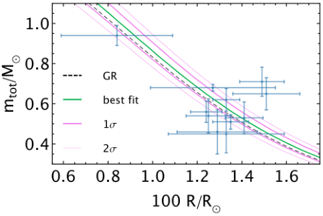
Finally, we move on to bounds set by the mass-radius relation of white dwarfs by comparing to the catalogue of stars in Holberg:2012pu. To simplify our analysis, we assume that the stars are each made of a low temperature, completely degenerate Fermi gas, and follow shapiro_teukolsky_1983. Practically speaking, this assumption means that the profile of the star is not significantly affected by the temperature, an assumption which is reasonable for Holberg:2012pu. For this reason, we omit the data point with in Holberg:2012pu. See Saltas:2018mxc for an example of a more involved analysis which includes these non-trivial temperature effects.
Under these assumptions, the equation of state of the star is given by,
| (90) | ||||
where , , and is the unitless Fermi momentum of an electron, which is in general a function of the distance from the center of the star, i.e. . The equation for hydrostatic equilibrium is the same as that mentioned above eq. (84), and combined with the mass conservation equation, , one obtains a system of first order differential equations for and .
After defining , , , and , this system can be written as
| (91) | ||||
The initial conditions are and (which determines the total mass of the star), and the radius of the star is given by . In particular, we have , and .
To do the fit to the data, we first find the points on the theoretical curve that match best with each data point . In particular, we define
| (92) |
where , , , and are respectively the mass, error bar for the mass, radius, and error bar for the radius of the th star, and we minimize each to find the where it is minimum. The total is then given by
| (93) |
where for us . We then minimize eq. (93) with respect to to find our constraints.
Calling the minimum, we then determine the region by finding where . In particular, we find a best fit value of , a range of , and a range of . We present our results in Fig. 2.
References
- (1) G. W. Horndeski, “Second-order scalar-tensor field equations in a four-dimensional space,” Int.J.Theor.Phys. 10 (1974) 363–384.
- (2) C. Deffayet, X. Gao, D. Steer, and G. Zahariade, “From k-essence to generalised Galileons,” Phys.Rev. D84 (2011) 064039, 1103.3260.
- (3) M. Zumalacárregui and J. García-Bellido, “Transforming gravity: from derivative couplings to matter to second-order scalar-tensor theories beyond the Horndeski Lagrangian,” Phys.Rev. D89 (2014), no. 6 064046, 1308.4685.
- (4) J. Gleyzes, D. Langlois, F. Piazza, and F. Vernizzi, “Healthy theories beyond Horndeski,” Phys. Rev. Lett. 114 (2015), no. 21 211101, 1404.6495.
- (5) D. Langlois and K. Noui, “Degenerate higher derivative theories beyond Horndeski: evading the Ostrogradski instability,” JCAP 1602 (2016), no. 02 034, 1510.06930.
- (6) M. Crisostomi, K. Koyama, and G. Tasinato, “Extended Scalar-Tensor Theories of Gravity,” JCAP 1604 (2016), no. 04 044, 1602.03119.
- (7) J. Ben Achour, M. Crisostomi, K. Koyama, D. Langlois, K. Noui, and G. Tasinato, “Degenerate higher order scalar-tensor theories beyond Horndeski up to cubic order,” JHEP 12 (2016) 100, 1608.08135.
- (8) D. Langlois, “Dark Energy and Modified Gravity in Degenerate Higher-Order Scalar-Tensor (DHOST) theories: a review,” 1811.06271.
- (9) T. Kobayashi, “Horndeski theory and beyond: a review,” 1901.07183.
- (10) C. M. Will, “The Confrontation between General Relativity and Experiment,” Living Rev.Rel. 17 (2014) 4, 1403.7377.
- (11) A. I. Vainshtein, “To the problem of nonvanishing gravitation mass,” Phys. Lett. 39B (1972) 393–394.
- (12) E. Babichev and C. Deffayet, “An introduction to the Vainshtein mechanism,” Class. Quant. Grav. 30 (2013) 184001, 1304.7240.
- (13) Virgo, LIGO Scientific Collaboration, B. P. Abbott et. al., “GW170817: Observation of Gravitational Waves from a Binary Neutron Star Inspiral,” Phys. Rev. Lett. 119 (2017), no. 16 161101, 1710.05832.
- (14) P. Creminelli and F. Vernizzi, “Dark Energy after GW170817 and GRB170817A,” Phys. Rev. Lett. 119 (2017), no. 25 251302, 1710.05877.
- (15) J. Sakstein and B. Jain, “Implications of the Neutron Star Merger GW170817 for Cosmological Scalar-Tensor Theories,” Phys. Rev. Lett. 119 (2017), no. 25 251303, 1710.05893.
- (16) J. M. Ezquiaga and M. Zumalacrregui, “Dark Energy After GW170817: Dead Ends and the Road Ahead,” Phys. Rev. Lett. 119 (2017), no. 25 251304, 1710.05901.
- (17) T. Baker, E. Bellini, P. G. Ferreira, M. Lagos, J. Noller, and I. Sawicki, “Strong constraints on cosmological gravity from GW170817 and GRB 170817A,” Phys. Rev. Lett. 119 (2017), no. 25 251301, 1710.06394.
- (18) C. de Rham and S. Melville, “Gravitational Rainbows: LIGO and Dark Energy at its Cutoff,” Phys. Rev. Lett. 121 (2018), no. 22 221101, 1806.09417.
- (19) J. Gleyzes, D. Langlois, F. Piazza, and F. Vernizzi, “Exploring gravitational theories beyond Horndeski,” JCAP 1502 (2015) 018, 1408.1952.
- (20) P. Creminelli, M. Lewandowski, G. Tambalo, and F. Vernizzi, “Gravitational Wave Decay into Dark Energy,” JCAP 1812 (2018), no. 12 025, 1809.03484.
- (21) B. Bellazzini, M. Lewandowski, and J. Serra, “Amplitudes’ Positivity, Weak Gravity Conjecture, and Modified Gravity,” 1902.03250.
- (22) A. Nicolis, R. Rattazzi, and E. Trincherini, “The Galileon as a local modification of gravity,” Phys. Rev. D79 (2009) 064036, 0811.2197.
- (23) T. Kobayashi, Y. Watanabe, and D. Yamauchi, “Breaking of Vainshtein screening in scalar-tensor theories beyond Horndeski,” Phys. Rev. D91 (2015), no. 6 064013, 1411.4130.
- (24) M. Crisostomi and K. Koyama, “Vainshtein mechanism after GW170817,” Phys. Rev. D97 (2018), no. 2 021301, 1711.06661.
- (25) D. Langlois, R. Saito, D. Yamauchi, and K. Noui, “Scalar-tensor theories and modified gravity in the wake of GW170817,” Phys. Rev. D97 (2018), no. 6 061501, 1711.07403.
- (26) A. Dima and F. Vernizzi, “Vainshtein Screening in Scalar-Tensor Theories before and after GW170817: Constraints on Theories beyond Horndeski,” 1712.04731.
- (27) N. Bartolo, P. Karmakar, S. Matarrese, and M. Scomparin, “Cosmic structures and gravitational waves in ghost-free scalar-tensor theories of gravity,” JCAP 1805 (2018), no. 05 048, 1712.04002.
- (28) A. Ganz, N. Bartolo, P. Karmakar, and S. Matarrese, “Gravity in mimetic scalar-tensor theories after GW170817,” JCAP 1901 (2019), no. 01 056, 1809.03496.
- (29) E. Babichev and A. Lehbel, “The sound of DHOST,” JCAP 1812 (2018), no. 12 027, 1810.09997.
- (30) R. Kase and S. Tsujikawa, “Dark energy scenario consistent with GW170817 in theories beyond Horndeski gravity,” Phys. Rev. D97 (2018), no. 10 103501, 1802.02728.
- (31) M. Crisostomi and K. Koyama, “Self-accelerating universe in scalar-tensor theories after GW170817,” Phys. Rev. D97 (2018), no. 8 084004, 1712.06556.
- (32) M. Crisostomi, K. Koyama, D. Langlois, K. Noui, and D. A. Steer, “Cosmological evolution in DHOST theories,” JCAP 1901 (2019), no. 01 030, 1810.12070.
- (33) N. Frusciante, R. Kase, K. Koyama, S. Tsujikawa, and D. Vernieri, “Tracker and scaling solutions in DHOST theories,” Phys. Lett. B790 (2019) 167–175, 1812.05204.
- (34) R. Kase and S. Tsujikawa, “Dark energy in Horndeski theories after GW170817: A review,” 1809.08735.
- (35) J. M. Ezquiaga and M. Zumalacrregui, “Dark Energy in light of Multi-Messenger Gravitational-Wave astronomy,” Front. Astron. Space Sci. 5 (2018) 44, 1807.09241.
- (36) C. de Rham and A. Matas, “Ostrogradsky in Theories with Multiple Fields,” JCAP 1606 (2016), no. 06 041, 1604.08638.
- (37) D. Langlois, M. Mancarella, K. Noui, and F. Vernizzi, “Effective Description of Higher-Order Scalar-Tensor Theories,” JCAP 1705 (2017), no. 05 033, 1703.03797.
- (38) E. Bellini and I. Sawicki, “Maximal freedom at minimum cost: linear large-scale structure in general modifications of gravity,” JCAP 1407 (2014) 050, 1404.3713.
- (39) P. Creminelli, G. D’Amico, J. Norena, and F. Vernizzi, “The Effective Theory of Quintessence: the Side Unveiled,” JCAP 0902 (2009) 018, 0811.0827.
- (40) G. D’Amico, Z. Huang, M. Mancarella, and F. Vernizzi, “Weakening Gravity on Redshift-Survey Scales with Kinetic Matter Mixing,” JCAP 1702 (2017) 014, 1609.01272.
- (41) G. Cusin, M. Lewandowski, and F. Vernizzi, “Nonlinear Effective Theory of Dark Energy,” JCAP 1804 (2018), no. 04 061, 1712.02782.
- (42) S. Hirano, T. Kobayashi, D. Yamauchi, and S. Yokoyama, “Constraining DHOST theories with linear growth of matter density fluctuations,” 1902.02946.
- (43) T. Kobayashi and T. Hiramatsu, “Relativistic stars in degenerate higher-order scalar-tensor theories after GW170817,” Phys. Rev. D97 (2018), no. 10 104012, 1803.10510.
- (44) J. Ben Achour, D. Langlois, and K. Noui, “Degenerate higher order scalar-tensor theories beyond Horndeski and disformal transformations,” Phys. Rev. D93 (2016), no. 12 124005, 1602.08398.
- (45) C. Brans and R. Dicke, “Mach’s principle and a relativistic theory of gravitation,” Phys.Rev. 124 (1961) 925–935.
- (46) S. M. Carroll, A. De Felice, V. Duvvuri, D. A. Easson, M. Trodden, and M. S. Turner, “The Cosmology of generalized modified gravity models,” Phys. Rev. D71 (2005) 063513, astro-ph/0410031.
- (47) J. Gleyzes, D. Langlois, M. Mancarella, and F. Vernizzi, “Effective Theory of Interacting Dark Energy,” JCAP 1508 (2015), no. 08 054, 1504.05481.
- (48) J. Beltran Jimenez, F. Piazza, and H. Velten, “Evading the Vainshtein Mechanism with Anomalous Gravitational Wave Speed: Constraints on Modified Gravity from Binary Pulsars,” Phys. Rev. Lett. 116 (2016), no. 6 061101, 1507.05047.
- (49) J. M. Weisberg, D. J. Nice, and J. H. Taylor, “Timing Measurements of the Relativistic Binary Pulsar PSR B1913+16,” Astrophys. J. 722 (2010) 1030–1034, 1011.0718.
- (50) R. A. Hulse and J. H. Taylor, “Discovery of a pulsar in a binary system,” Astrophys. J. 195 (1975) L51–L53.
- (51) B. Bertotti, L. Iess, and P. Tortora, “A test of general relativity using radio links with the Cassini spacecraft,” Nature 425 (2003) 374–376.
- (52) I. D. Saltas, I. Sawicki, and I. Lopes, “White dwarfs and revelations,” JCAP 1805 (2018), no. 05 028, 1803.00541.
- (53) S. Hirano, T. Kobayashi, and D. Yamauchi, “On the screening mechanism in DHOST theories evading gravitational wave constraints,” 1903.08399.
- (54) S. Chandrasekhar and E. A. Milne, “The Highly Collapsed Configurations of a Stellar Mass,” Mon. Not. Roy. Astron. Soc. 91 (1931), no. 5 456–466.
- (55) S. Chandrasekhar, “The highly collapsed configurations of a stellar mass (Second paper),” Mon. Not. Roy. Astron. Soc. 95 (1935) 207–225.
- (56) R. K. Jain, C. Kouvaris, and N. G. Nielsen, “White Dwarf Critical Tests for Modified Gravity,” Phys. Rev. Lett. 116 (2016), no. 15 151103, 1512.05946.
- (57) A. Burrows and J. Liebert, “The Science of brown dwarfs,” Rev. Mod. Phys. 65 (1993) 301–336.
- (58) J. Sakstein, “Hydrogen Burning in Low Mass Stars Constrains Scalar-Tensor Theories of Gravity,” Phys. Rev. Lett. 115 (2015) 201101, 1510.05964.
- (59) D. Segransan, X. Delfosse, T. Forveille, J. L. Beuzit, S. Udry, C. Perrier, and M. Mayor, “Accurate masses of very low mass stars. 3. 16 New or improved masses,” Astron. Astrophys. 364 (2000) 665, astro-ph/0010585.
- (60) R. S. Freedman, M. S. Marley, and K. Lodders, “Line and Mean Opacities for Ultracool Dwarfs and Extrasolar Planets,” Astrophys. J. Suppl. 174 (2008) 504, 0706.2374.
- (61) J. B. Holberg, T. D. Oswalt, and M. A. Barstow, “Observational Constraints on the Degenerate Mass-Radius Relation,” Astron. J. 143 (2012) 68, 1201.3822.
- (62) S. A. Shapiro, Stuart L.; Teukolsky, Black Holes, White Dwarfs, and Neutron Stars. Wiley-Interscience, 1983.