A Method for Convex Black-Box Integer Global Optimization

Jeffrey Larson Sven Leyffer Prashant Palkar Stefan M. Wild

Abstract

We study the problem of minimizing a convex function on a nonempty, finite subset of the integer lattice when the function cannot be evaluated at noninteger points. We propose a new underestimator that does not require access to (sub)gradients of the objective but, rather, uses secant linear functions that interpolate the objective function at previously evaluated points. These linear mappings are shown to underestimate the objective in disconnected portions of the domain. Therefore, the union of these conditional cuts provides a nonconvex underestimator of the objective. We propose an algorithm that alternates between updating the underestimator and evaluating the objective function. We prove that the algorithm converges to a global minimum of the objective function on the feasible set. We present two approaches for representing the underestimator and compare their computational effectiveness. We also compare implementations of our algorithm with existing methods for minimizing functions on a subset of the integer lattice. We discuss the difficulty of this problem class and provide insights into why a computational proof of optimality is challenging even for moderate problem sizes.

1 Introduction

We study the problem of minimizing a convex function on a finite subset of the integer lattice. In particular, we consider problems of the form

\mathop{\mbox{minimize}}_{x}\;f(x)\quad\mbox{subject to }\;x\in\Omega\subset\mathbb{Z}^{n}.

(1)

We first define what it means for $f$ to be convex on a set $\Omega\subset\mathbb{Z}^{n}$ .

Definition 1 (Convexity on Integer Subsets).

A function $f$ is convex on $\Omega$ if for $x\in\Omega$ and any $p$ points $y^{i}\in\Omega$ satisfying $x=\sum_{i=1}^{p}\lambda_{i}y^{i}$ with $\lambda_{i}\in[0,1]$ and $\sum_{i=1}^{p}\lambda_{i}=1$ , then $f(x)\leq\sum_{i=1}^{p}\lambda_{i}f(y^{i})$ .

We make the following assumption about problem (1).

Assumption 1.

$f$ is convex on $\Omega$ , $\Omega\subset\mathbb{Z}^{n}$ is nonempty and bounded, and $f$ cannot be evaluated at $x\notin\Omega$ .

Because we assume that $f$ cannot be evaluated at noninteger points, problem (1) can be referred to as a convex optimization problem with unrelaxable integer constraints [30]. We note that $\Omega$ need not contain all integer points in its convex hull (i.e., our approach allows for situations where $\mathrm{conv}\left(\Omega\right)\cap\mathbb{Z}^{n}\not=\Omega$ ). Problem (1) can also be viewed as minimizing an integer-convex¹¹ 1 Although [24] considers integer convexity only for polynomials, this definition can be applied to more general classes of functions over the sets considered here. function [24, Definition 15.2] over a nonempty finite subset of $\mathbb{Z}^{n}$ .

Admittedly, it is rare to know that $f$ is convex when $f$ is not given in closed form (although one may be able to detect convexity [27] or estimate a probability that $f$ is convex on the finite domain $\Omega$ [26]). Nevertheless, studying the convex case is important because we are unaware of any method (besides complete enumeration) for obtaining exact solutions to (1) when $f$ (convex or otherwise) cannot be evaluated at noninteger points.

One example where an objective is not given in closed form but is known to be convex arises in the combinatorial optimal control of partial differential equations (PDEs). For example, Buchheim et al. [9, Lemma 2] show that the solution operator of certain semilinear elliptic PDEs is a convex function of the controls provided that the nonlinearities in the PDE and boundary conditions are concave and nondecreasing. Thus, any linear function of the states of the PDE (e.g., the $\max$ -function) is a convex function of the controls when the states are eliminated. The authors of [9] propose using adjoint information to compute subgradients of the (continuous relaxation of the) objective, but an alternative would be to consider a derivative-free approach.

We consider only pure-integer problems of the form (1); however, our developments are equally applicable to the mixed-integer case

\mathop{\mbox{minimize}}_{x,y}\;F(x,y)\quad\mbox{subject to }\;(x,y)\in\Omega\times\Psi\subset\mathbb{Z}^{n}\times\mathbb{R}^{m}

(2)

provided $F$ is convex on $\Omega\times\Psi$ . If we define the function

f(x)=\min_{y\in\Psi}F(x,y)

and if $f$ is well defined over $\Omega$ , then (2) can be solved by minimizing $f$ on $\Omega\subset\mathbb{Z}^{n}$ , where each evaluation $f(x)$ requires an optimization of the continuous variables $y$ for a fixed $x$ . (When there is no additional information on $F$ and $\Psi$ , each continuous optimization problem may be difficult to solve.) Because many of the results below rely only on the convexity of $f$ and not the discrete nature of $\Omega$ , much of the analysis below readily applies to the mixed-integer case.

We are especially interested in problems where the cost of evaluating $f$ is large. Problems of the form (1) or (2) where the objective is expensive to evaluate and some integer constraints are unrelaxable arise in a range of simulation-based optimization problems. For example, the optimal design of concentrating solar power plants gives rise to computationally expensive simulations for each set of design parameters [41]. Furthermore, some of the design parameters (e.g., the number of panels on the power plant receiver) cannot be relaxed to noninteger values. Similar problems arise when tuning codes to run on high-performance computers [6]. In this case, $f(x)$ may be the memory footprint of a code that is compiled with settings $x$ , which can correspond to decisions such as loop unrolling or tiling factors that do not have meaningful noninteger values. Optimal material design problems may also constrain the choice of atoms to a finite set, resulting in unrelaxable integer constraints; see [21] for a derivative-free optimization algorithm designed explicitly for such a problem.

Motivated by such applications, we develop a method that will certifiably converge to the solution of (1) under Assumption 1 without access to $\partial f$ . Using only evaluations of $f$ , we construct secants, which are linear functions that interpolate $f$ at a set of $n+1$ points. These secant functions underestimate $f$ in certain parts of $\Omega$ . We use these secants to define conditional cuts that are valid in disconnected portions of the domain. The complete set of secants and the conditions that describe when they are valid are used to construct an underestimator of a convex $f$ . While access to $\partial f$ (i.e., a (sub)gradient of a continuous relaxation of $f$ ) could strengthen such an underestimator, we do not address such considerations in this paper.

Solving (1) under Assumption 1 without access to $\partial f$ poses a number of theoretical and computational challenges. Because the integer constraints are unrelaxable, one cannot apply traditional branch-and-bound approaches. In particular, model-based continuous derivative-free methods would require evaluating the objective at noninteger points to ensure convergence for the continuous relaxation of (1). In addition, other traditional techniques for mixed-integer optimization—such as Benders decomposition [20] or outer approximation [17, 18]—cannot be used to solve (1) when $\partial f$ is unavailable. Since we know of no method (other than complete enumeration) for obtaining global minimizers of (1) under Assumption 1, we know of no potential algorithm to address this problem when a (sub)gradient is unavailable.

We make three contributions in this paper: (1) we develop a new underestimator for convex functions on subsets of the integer lattice that is based solely on function evaluations; (2) we present an algorithm that alternates between updating this underestimator and evaluating the objective in order to identify a global solution of problem (1) under Assumption 1; and (3) we show empirically that certifying global optimality in such cases is a challenging problem. In our experiments, we are unable to prove optimality for many problems when $n\geq 5$ , and we provide insights into why a proof of optimality remains computationally challenging.

Outline.

Section 2 surveys recent methods for addressing (1). Section 3 introduces valid conditional cuts using only the function values of a convex objective and discusses the theoretical properties of these cuts. Section 4 presents an algorithm for solving (1) and shows that this algorithm identifies a global minimizer of (1) under Assumption 1. Section 5 considers two approaches for formulating the underestimator and presents the method SUCIL—secant underestimator of convex functions on the integer lattice. Section 6 provides detailed numerical studies for implementations of SUCIL on a set of convex problems. Section 7 discusses many of the challenges in obtaining global solutions to (1).

2 Background

Developing methods to solve (1) without access to derivatives of $f$ is an active area of research. Most methods address general (i.e., nonconvex) functions $f$ , and heuristic approaches are commonly adopted to handle integer decision variables for such derivative-free optimization problems. For example, the method in [37] rounds noninteger components of candidate points to the nearest feasible integer values. The method’s asymptotic convergence results are based on the inclusion of points drawn uniformly from the finite domain (and rounding noninteger values as necessary).

Integer-constrained pattern-search methods [2, 4] generalize their continuous counterparts. These modified pattern-search methods can be shown to converge to mesh-isolated minimizers: points with function values that are better than all neighboring points on the integer lattice. Unfortunately, such mesh-isolated minimizers can be arbitrarily far from a global minimizer, even when $f$ is convex; see [1, Fig. 2] for an example of such a function $f$ . Other methods that converge to mesh-isolated minimizers include direct-search methods that update the integer variables via a local search [31, 32] and mesh adaptive direct-search methods adapted to address discrete and granular variables (i.e., those that have a controlled number of decimals) [3, 5]. The direct-search method in [19] accounts for integer constraints by constructing a set of directions that have a nonnegative span of $\mathbb{R}^{n}$ and that ensure that all evaluated points will be integer valued. This method is shown to converge to a type of stationary point that, even in the convex case, may not be a global minimizer. See [38] for various definitions of local minimizers of (1) and a discussion of associated properties. The BFO method in [39] has a recursive step that explores points near the current iterate by fixing each of the discrete variables to its value plus or minus a step-size parameter.

[Uncaptioned image] — Table 1: Number of primitive directions, $\#=\lvert\mathcal{N}(x_{c},1)\rvert$ , that emanate from the origin $x_{c}$ of the domain ${\Omega=\left[-k,k\right]^{n}\cap\mathbb{Z}^{n}}$ and that correspond to points in $\Omega$ .

	$n=2$	$n=3$	$n=4$	$n=5$
1	9	8	27	26	81	80	243	242
2	25	16	125	98	625	544	3,125	2,882
3	49	32	343	290	2,403	2,240	16,807	16,322
4	81	48	729	578	6,561	5,856	59,049	55,682

The method in [33] uses line searches over a set of primitive directions, that is, a set of scaled directions $D$ where no vector $d_{i}\in D$ is a positive multiple of a different $d_{j}\in D$ . This method explores a discrete set of directions around the current iterate until finding a local minimum $x_{c}$ in a $\beta$ -neighborhood, defined as $\mathcal{N}(x_{c},\beta)=\{x_{c}+\alpha d\in\Omega:d\in D,\alpha\in\mathbb{N},\alpha\leq\beta\}$ for $\beta\in\mathbb{N}$ . Although the authors of [33] target nonconvex objectives, their approach will converge to a global minimum $x_{c}$ of a convex objective $f$ if all points in $\mathcal{N}(x_{c},1)$ are evaluated. Figure 1 illustrates such a discrete 1-neighborhood. Unfortunately, $|\mathcal{N}(x_{c},1)|$ can be large; see Table 1.

Model-based methods approximate objective functions on the integer lattice by using surrogate models; see, for example, [25], [40], and [13]. The surrogate model is used to determine points where the objective should be evaluated; the model is typically refined after each objective evaluation. The methodology in [13] specifically uses radial basis function surrogate models and does automatic model selection at each iteration. Mixed-integer nonlinear optimization solvers are used to minimize the surrogate to obtain the next integer point for evaluation. The model-based methods of [34, 35, 36] modify the sampling strategies and local searches typically used to solve continuous objective versions. The approaches in [34, 35] restart when a suitably defined local minimizer is encountered, continuing to evaluate the objective until the available budget of function evaluations is exhausted. These model-based methods differ in the initial sampling method, the type of surrogate model, and the sampling strategy used to select the next points to be evaluated. See [7], for a survey and taxonomy of continuous and integer model-based optimization approaches.

In a different line of research, Davis and Ierapetritou [14] propose a branch-and-bound framework to address binary variables; a solution to the relaxed nonlinear subproblems is obtained via a combination of global kriging models and local surrogate models. Similarly, Hemker et al. [23] replace the black-box portions of the objective function (and constraints) by a stochastic surrogate; the resulting mixed-integer nonlinear programs are solved by branch and bound. Both approaches assume that the integer constraints are relaxable.

3 Underestimator of Convex Functions on the Integer Lattice

To construct an underestimator of a convex objective function $f$ , we now discuss secant functions, which are linear mappings that interpolate $f$ at $n+1$ points. We provide conditions for where these cuts will underestimate $f$ . We then discuss necessary conditions on the set of evaluated points so that if all possible secants are constructed, these conditional cuts underestimate $f$ on the domain $\Omega$ . As we will see in Section 4, this underestimator is essential for obtaining a global minimizer of (1) under Assumption 1. Throughout this section, $X\subseteq\Omega$ denotes a set of at least $n+1$ points in $\Omega$ at which the objective function $f$ has been evaluated.

3.1 Secant Functions and Conditional Cuts

Constructing a secant function requires a set of $n+1$ interpolation points where $f$ has been evaluated. To define a secant function for $f$ , we introduce a multi-index $i$ of $n+1$ distinct indices, $1\leq i_{1}<\ldots<i_{n+1}\leq\left|X\right|$ , as $\mbox{\boldmath$i$}=(i_{1},\ldots,i_{n+1})$ . With a slight abuse of notation, we will refer to elements $i_{j}\in\mbox{\boldmath$i$}$ .

Given the set of points $X^{\mbox{\boldmath$i$}}=\left\{x^{i_{j}}\in X\subseteq\Omega:i_{j}\in\mbox{\boldmath$i$}\right\}$ , we construct the secant function

m^{\mbox{\boldmath$i$}}(x)=(c^{\mbox{\boldmath$i$}})^{\operatorname{T}}x+b^{\mbox{\boldmath$i$}},

where the coefficients $c^{\mbox{\boldmath$i$}}\in\mathbb{R}^{n}$ and $b^{\mbox{\boldmath$i$}}\in\mathbb{R}$ are the solution to the linear system

\left[\bar{X}^{\mbox{\boldmath$i$}}\;e\right]\left[\begin{array}[]{l}c^{\mbox{\boldmath$i$}}\\ b^{\mbox{\boldmath$i$}}\end{array}\right]=f^{\mbox{\boldmath$i$}},\;\text{where}\;\bar{X}^{\mbox{\boldmath$i$}}=\left[\begin{array}[]{c}(x^{i_{1}})^{\operatorname{T}}\\ \vdots\\ (x^{i_{n+1}})^{\operatorname{T}}\end{array}\right],\;e=\left[\begin{array}[]{c}1\\ \vdots\\ 1\end{array}\right],\;\mbox{and}\;f^{\mbox{\boldmath$i$}}=\left[\begin{array}[]{c}f(x^{i_{1}})\\ \vdots\\ f(x^{i_{n+1}})\end{array}\right].

(3)

The secant function $m^{\mbox{\boldmath$i$}}$ is unique provided that the set $X^{\mbox{\boldmath$i$}}$ is poised, which we now define.

Definition 2.

The set of points $X^{\mbox{\boldmath$i$}}$ is poised if the matrix $\left[\bar{X}^{\mbox{\boldmath$i$}}\;e\right]$ is nonsingular.

Note that Definition 2 is equivalent to $X^{\mbox{\boldmath$i$}}$ being affinely independent. We now show that the secant function $m^{\mbox{\boldmath$i$}}$ underestimates $f$ in certain polyhedral cones, namely, the cones

\mathcal{U}^{\mbox{\boldmath$i$}}=\bigcup\limits_{i_{j}\in\mbox{\boldmath$i$}}\mathrm{cone}\big(x^{i_{j}}-X^{\mbox{\boldmath$i$}}\big),

(4)

where

\mathrm{cone}\big(x^{i_{j}}-X^{\mbox{\boldmath$i$}}\big)=\{x^{i_{j}}+\sum_{l=1,l\neq j}^{n+1}\lambda_{l}(x^{i_{j}}-x^{i_{l}}):\,i_{j}\in\mbox{\boldmath$i$},i_{l}\in\mbox{\boldmath$i$},\lambda_{l}\geq 0\}.

(5)

Lemma 1 (Conditional Cuts).

If $f$ is convex on $\Omega$ and $X^{\mbox{\boldmath$i$}}$ $\subseteq\Omega$ is poised, then the unique linear mapping $m^{\mbox{\boldmath$i$}}$ satisfying $m^{\mbox{\boldmath$i$}}(x^{i_{j}})=f(x^{i_{j}})$ for each $i_{j}\in\mbox{\boldmath$i$}$ satisfies $m^{\mbox{\boldmath$i$}}(x)\leq f(x)$ for all $x\in\mathcal{U}^{\mbox{\boldmath$i$}}\bigcap\Omega$ .

Proof.

The uniqueness of the linear mapping follows directly from the affine independence guaranteed by Definition 2 for poised $X^{\mbox{\boldmath$i$}}$ .

Let $x$ be a point in $\mathrm{cone}\big(x^{i_{j}}-X^{\mbox{\boldmath$i$}}\big)\bigcap\Omega$ for arbitrary $x^{i_{j}}\in X^{\mbox{\boldmath$i$}}$ . By (5),

x=x^{i_{j}}+\sum_{l=1,l\neq j}^{n+1}\lambda_{l}\left(x^{i_{j}}-x^{i_{l}}\right),

(6)

with $\lambda_{l}\geq 0$ (for $l=1,\ldots,n+1;l\neq j$ ). Rearranging (6) yields

x^{i_{j}}=\frac{1}{1+\sum_{k=1,k\neq j}^{n+1}\lambda_{k}}x+\frac{1}{1+\sum_{k=1,k\neq j}^{n+1}\lambda_{k}}\sum_{l=1,l\neq j}^{n+1}\lambda_{l}x^{i_{l}},

showing that $x^{i_{j}}$ can be expressed as a convex combination of $\{x\}\cup\{x^{i_{l}}:l=1,\ldots,n+1;l\neq j\}$ , all of which are points in $\Omega$ . Therefore, by convexity of $f$ on $\Omega$ (see Definition 1),

f(x^{i_{j}})\leq\frac{1}{1+\sum_{k=1,k\neq j}^{n+1}\lambda_{k}}f(x)+\frac{1}{1+\sum_{k=1,k\neq j}^{n+1}\lambda_{k}}\sum_{l=1,l\neq j}^{n+1}\lambda_{l}f\left(x^{i_{l}}\right).

Solving for $f(x)$ and using the fact that $m^{\mbox{\boldmath$i$}}$ interpolates $f$ at points in $X^{\mbox{\boldmath$i$}}$ , we obtain

	$\displaystyle f(x)$	$\displaystyle\geq\left(1+\sum_{k=1,k\neq j}^{n+1}\lambda_{k}\right)f(x^{i_{j}})-\sum_{l=1,l\neq j}^{n+1}\lambda_{l}f(x^{i_{l}})$
		$\displaystyle=\left(1+\sum_{k=1,k\neq j}^{n+1}\lambda_{k}\right)m^{\mbox{\boldmath$i$}}(x^{i_{j}})-\sum_{l=1,l\neq j}^{n+1}\lambda_{l}m^{\mbox{\boldmath$i$}}(x^{i_{l}})$
		$\displaystyle=m^{\mbox{\boldmath$i$}}(x^{i_{j}})+\sum_{l=1,l\neq j}^{n+1}\lambda_{l}\left(m^{\mbox{\boldmath$i$}}(x^{i_{j}})-m^{\mbox{\boldmath$i$}}(x^{i_{l}})\right)$
		$\displaystyle=m^{\mbox{\boldmath$i$}}(x),$

where the last equality holds by (6) and the linearity of $m^{\mbox{\boldmath$i$}}$ . Because $x$ is an arbitrary point in $\mathrm{cone}\big(x^{i_{j}}-X^{\mbox{\boldmath$i$}}\big)$ for arbitrary $x^{i_{j}}$ , the result is shown. ∎

We now prove that the cones in $\mathcal{U}^{\mbox{\boldmath$i$}}$ do not intersect when $X^{\mbox{\boldmath$i$}}$ is poised. We note that the following result holds for any poised set $X^{\mbox{\boldmath$i$}}\subset\mathbb{R}^{n}$ .

Lemma 2 (A Point Is In At Most One Cone).

If $X^{\mbox{\boldmath$i$}}$ is poised, no point $x\in\mathbb{R}^{n}$ satisfies $x\in\mathrm{cone}\big(x^{i_{j}}-X^{\mbox{\boldmath$i$}}\big)$ and $x\in\mathrm{cone}\big(x^{i_{k}}-X^{\mbox{\boldmath$i$}}\big)$ for $x^{i_{j}},x^{i_{k}}\in X^{\mbox{\boldmath$i$}}$ and $x^{i_{j}}\neq x^{i_{k}}$ .

Proof.

Let $x^{i_{1}}$ and $x^{i_{2}}$ be different, but otherwise arbitrary, points in $X^{\mbox{\boldmath$i$}}$ . To arrive at a contradiction, suppose that there exists $x\in\mathrm{cone}\big(x^{i_{1}}-X^{\mbox{\boldmath$i$}}\big)\cap\mathrm{cone}\big(x^{i_{2}}-X^{\mbox{\boldmath$i$}}\big)$ . That is, $x=x^{i_{1}}+\sum_{l=2}^{n+1}\lambda_{l}\left(x^{i_{1}}-x^{i_{l}}\right)$ and $x=x^{i_{2}}+\sum_{l=1,l\neq 2}^{n+1}\sigma_{l}\left(x^{i_{2}}-x^{i_{l}}\right)$ for $\lambda_{l}\geq 0$ ( $l\in\left\{2,\ldots,n+1\right\}$ ) and $\sigma_{l}\geq 0$ ( $l\in\left\{1,3,\ldots,n+1\right\}$ ). Subtracting these two expressions yields

$\displaystyle 0$	$\displaystyle=x^{i_{1}}-x^{i_{2}}+\sum_{l=2}^{n+1}\lambda_{l}(x^{i_{1}}-x^{i_{l}})-\sum_{l=1,l\neq 2}^{n+1}\sigma_{l}(x^{i_{2}}-x^{i_{l}})$
	$\displaystyle=x^{i_{1}}-x^{i_{2}}+\sum_{l=2}^{n+1}\lambda_{l}x^{i_{1}}-\sum_{l=2}^{n+1}\lambda_{l}x^{i_{2}}+\sum_{l=2}^{n+1}\lambda_{l}x^{i_{2}}-\sum_{l=2}^{n+1}\lambda_{l}x^{i_{l}}-\sum_{l=1,l\neq 2}^{n+1}\sigma_{l}(x^{i_{2}}-x^{i_{l}})$
	$\displaystyle=\left(1+\sum_{l=2}^{n+1}\lambda_{l}\right)\left(x^{i_{1}}-x^{i_{2}}\right)-\sum_{l=2}^{n+1}\lambda_{l}\left(x^{i_{l}}-x^{i_{2}}\right)+\sum_{l=1,l\neq 2}^{n+1}\sigma_{l}\left(x^{i_{l}}-x^{i_{2}}\right)$
	$\displaystyle=\left(1+\sigma_{1}+\sum_{l=2}^{n+1}\lambda_{l}\right)\left(x^{i_{1}}-x^{i_{2}}\right)+\sum_{l=3}^{n+1}\left(\sigma_{l}-\lambda_{l}\right)\left(x^{i_{l}}-x^{i_{2}}\right).$	(7)

Since $X^{\mbox{\boldmath$i$}}$ is a poised set, Definition 2 ensures that the vectors $\left\{x^{i_{l}}-x^{i_{2}}:\,i_{l}\in\mbox{\boldmath$i$},i_{l}\neq i_{2}\right\}$ are linearly independent. Hence the dependence relation in (3.1) can be satisfied only if the coefficient on $(x^{i_{1}}-x^{i_{2}})$ vanishes. That is,

1+\sigma_{1}+\sum_{l=2}^{n+1}\lambda_{l}=0,

which contradicts $\lambda_{l}\geq 0$ (for $l=2,\ldots,n+1$ ) and $\sigma_{1}\geq 0$ . Since $x^{i_{1}}$ and $x^{i_{2}}$ were arbitrary points in $X^{\mbox{\boldmath$i$}}$ , the result is shown. ∎

For each poised set $X^{\mbox{\boldmath$i$}}$ , Lemma 1 ensures that the secant function $m^{\mbox{\boldmath$i$}}$ underestimates $f$ on $\Omega\cap\mathcal{U}^{\mbox{\boldmath$i$}}$ . We can therefore underestimate $f$ via a model that consists of the pointwise maximum of the underestimators for which the point is in $\mathcal{U}^{\mbox{\boldmath$i$}}$ for some poised set $X^{\mbox{\boldmath$i$}}$ of previously evaluated points. Minimizing this nonconvex model on the integer $\Omega$ can then provide a lower bound for the global minimum of $f$ on $\Omega$ .

Figure 1: Illustration of areas in

\mathbb{R}^{2}

where conditional cuts are valid. Left shows the regions of the domain where the secant through three points (the vertices of the blue triangle) will underestimate

f

. Right shows that one point in the interior of

n+1

points is sufficient to underestimate

f

. The conditional cuts correspond to the

n+1

points in the triangle of the same color.

Figure 1 shows a two-dimensional example of points that produce such secant functions and the regions in which they will underestimate any convex function $f$ . For the $n+2$ points (circles), we consider three poised sets indicated by triangles linking $n+1$ points. The left image shows a poised set (blue line triangle), and the three cones (shaded blue area) in which the secant through these points is a valid underestimator. The right image shows that conditional cuts using $n+2$ points can cover all of $\mathbb{R}^{n}$ .

3.2 Lower Bound for $f$

We now describe an optimization problem whose solution provides a lower bound for $f$ on $\Omega$ . Let $W(X)$ denote the set of all multi-indices corresponding to poised subsets of $X$ :

W(X)=\left\{\mbox{\boldmath$i$}:X^{\mbox{\boldmath$i$}}\subseteq X,X^{\mbox{\boldmath$i$}}\mbox{ is poised}\right\}.

(8)

If $f$ has been evaluated at every point in $X$ , we can construct a secant function $(c^{\mbox{\boldmath$i$}})^{\operatorname{T}}x+b^{\mbox{\boldmath$i$}}$ interpolating $f$ on $X^{\mbox{\boldmath$i$}}$ for every multi-index $\mbox{\boldmath$i$}\in W(X)$ . We then collect all such conditional cuts in the piecewise linear program

$\displaystyle\displaystyle\mathop{\mbox{minimize}}_{x,\eta}$	$\displaystyle\eta$	(PLP)
$\displaystyle\mbox{subject to }$	$\displaystyle\displaystyle\eta\geq(c^{\mbox{\boldmath$i$}})^{\operatorname{T}}x+b^{\mbox{\boldmath$i$}},\text{ for all }\mbox{\boldmath$i$}\in W(X)\text{ with }x\in\mathcal{U}^{\mbox{\boldmath$i$}}$
	$\displaystyle\displaystyle x\in\Omega,$

where $\mathcal{U}^{\mbox{\boldmath$i$}}$ is defined in (4). For the set of points $X$ and corresponding $W(X)$ , let $\eta(\bar{x})$ denote the value of (PLP) when the constraint $x=\bar{x}$ is added to (PLP) for a particular $\bar{x}\in\Omega$ . As we will see below, $\eta$ represents the largest lower bound for $f$ induced by the set $X$ , and the solution to (PLP) provides a lower bound for $f$ on $\Omega$ .

Lemma 3 (Underestimator of $f$ ).

If $f$ is convex on $\Omega$ , then the optimal value $\eta_{*}$ of (PLP) satisfies $\eta_{*}\leq f(x)$ for all $x\in\Omega$ .

Proof.

If $W(X)$ is empty, the result holds trivially since $\eta$ is unconstrained. Otherwise, since (PLP) minimizes $\eta$ , it suffices to show that $\eta(x)\leq f(x)$ for arbitrary $x\in\Omega$ . Two cases can occur. First, if $x\notin\mathcal{U}^{\mbox{\boldmath$i$}}$ for every $\mbox{\boldmath$i$}\in W(X)$ , then no conditional cut exists at $x$ . Thus $\eta(x)=-\infty$ and $\eta(x)<f(x)$ . Second, if $x\in\mathcal{U}^{\mbox{\boldmath$i$}}$ for some $\mbox{\boldmath$i$}\in W(X)$ , then

(c^{\mbox{\boldmath$i$}})^{\operatorname{T}}x+b^{\mbox{\boldmath$i$}}\leq f(x),

by Lemma 1, where the poisedness of $X^{\mbox{\boldmath$i$}}$ follows from the definition of $W(X)$ . Therefore, $\eta(x)\leq f(x)$ for all $x\in\Omega$ . Since $\eta_{*}=\displaystyle\min_{x\in\Omega}\eta(x)$ , the result is shown. ∎

If $W(X)$ in (PLP) is replaced by a proper subset $W^{\prime}(X)\subset W(X)$ of multi-indices, then Lemma 3 still holds. (This relaxation of (PLP) associated with removing constraints cannot increase $\eta_{*}$ .) Such a replacement may be necessary if $W(X)$ becomes too large to allow considering every poised subset of $X$ when forming (PLP).

3.3 Covering $\mathbb{R}^{n}$ with Conditional Cuts

Because the cuts in (PLP) are valid only within $\mathcal{U}^{\mbox{\boldmath$i$}}$ , the resulting model takes an optimal value of $\eta_{*}=-\infty$ if there is a point $x\in\Omega$ that is not in the union of $\mathcal{U}^{\mbox{\boldmath$i$}}$ over all $\mbox{\boldmath$i$}\in W(X)$ . Thus, we find it beneficial to ensure that $X$ contains points that result in a finite objective value for the underestimator described by (PLP). We now establish a condition that ensures that the union of conditional cuts induced by $X$ covers $\mathbb{R}^{n}$ and therefore $\Omega$ .

We say that a point $x^{0}$ belongs to the interior of the convex hull of a set of points $X=\{x^{1},\ldots,x^{n+1}\}$ if scalars $\alpha_{j}$ exist such that

x^{0}=\sum_{j=1}^{n+1}\alpha_{j}x^{j},\mbox{ where }\sum_{j=1}^{n+1}\alpha_{j}=1\mbox{ and }\alpha_{j}>0\mbox{ for }j=1,\ldots,n+1.

(9)

This is denoted by $x^{0}\in\mathrm{int}\left(\mathrm{conv}\left(X\right)\right)$ .

Lemma 4 (Poisedness of Initial Points).

If $X=\{x^{1},\ldots,x^{n+1}\}\subset\mathbb{R}^{n}$ is a poised set and if $x^{0}$ satisfies $x^{0}\in\mathrm{int}\left(\mathrm{conv}\left(X\right)\right)$ , then all subsets of $n+1$ points in $\{x^{0}\}\cup X$ are poised.

Proof.

For contradiction, suppose that the set $\{x^{0}\}\cup X\setminus\{x^{n+1}\}$ is not poised and therefore is affinely dependent. Then, there must exist scalars $\beta_{j}$ not all zero, and (without loss of generality) $x^{n}\in X$ such that

\sum_{j=0}^{n-1}\beta_{j}(x^{j}-x^{n})=0.

(10)

Replacing $x^{0}$ with (9) in the left-hand side above yields

	$\displaystyle 0$	$\displaystyle=\beta_{0}\left(\sum_{j=1,j\neq n}^{n+1}\alpha_{j}x^{j}+(\alpha_{n}-1)x^{n}\right)+\sum_{j=1}^{n-1}\beta_{j}(x^{j}-x^{n})$
		$\displaystyle=\sum_{j=1}^{n-1}(\beta_{0}\alpha_{j}+\beta_{j})x^{j}+\bigg(\beta_{0}(\alpha_{n}-1)-\sum_{j=1}^{n-1}\beta_{j}\bigg)x^{n}+\beta_{0}\alpha_{n+1}x^{n+1}.$		(11)

Since $X$ is poised, the vectors $\{x^{1},\ldots,x^{n+1}\}$ are affinely independent; by definition of affine independence, the only solution to $\sum_{j=1}^{n+1}\gamma_{j}x^{j}=0$ and $\sum_{j=1}^{n+1}\gamma_{j}=0$ is $\gamma_{j}=0$ for $j=1,\ldots,n+1$ . The sum of the coefficients from (3.3) satisfies

\sum_{j=1}^{n-1}(\beta_{0}\alpha_{j}+\beta_{j})+\beta_{0}(\alpha_{n}-1)-\sum_{j=1}^{n-1}\beta_{j}+\beta_{0}\alpha_{n+1}=\beta_{0}\sum_{j=1}^{n+1}\alpha_{j}-\beta_{0}=0,

because $\sum_{j=1}^{n+1}\alpha_{j}=1$ . This means that all coefficients of $x^{j}$ in (3.3) are also equal to zero. Since $\alpha_{n+1}>0$ , the last term from (3.3) implies that $\beta_{0}=0$ . Considering the remaining coefficients in (3.3), we conclude that $\beta_{0}\alpha_{j}+\beta_{j}=0$ , which implies that $\beta_{j}=0$ for $j=1,\ldots,n-1$ . This contradicts the assumption that not all $\beta_{j}=0$ . Hence, the result is proved. ∎

We now establish a simple set of points that produces conditional cuts that cover $\mathbb{R}^{n}$ and, therefore, the domain $\Omega$ .

Lemma 5 (Initial Points and Coverage of $\Omega$ ).

Let $X$ be a poised set of $n+1$ points, let $x^{0}\in\mathrm{int}\left(\mathrm{conv}\left(X\right)\right)$ , and let $W(X\cup\{x^{0}\})$ be defined as in (8). Then,

\bigcup\limits_{\mbox{\boldmath$i$}\in W(X\cup\{x^{0}\})}\mathcal{U}^{\mbox{\boldmath$i$}}=\mathbb{R}^{n}.

Proof.

Since $x^{0}\in\mathrm{int}\left(\mathrm{conv}\left(X\right)\right)$ , there exist $\alpha_{j}>0$ such that

0=(\sum_{j=1}^{n+1}\alpha_{j})(x^{0}-x^{0})=(\sum_{j=1}^{n+1}\alpha_{j})x^{0}-\sum_{j=1}^{n+1}\alpha_{j}x^{j}=\sum_{j=1}^{n+1}\alpha_{j}(x^{0}-x^{j}),

(12)

where the second equality follows from (9). The existence of $\alpha_{j}>0$ such that $\sum_{j=1}^{n+1}\alpha_{j}(x^{0}-x^{j})=0$ implies that the vectors $\left\{x^{0}-x^{j}:j\in\{1,\ldots,n+1\}\right\}$ are a positive spanning set (see, e.g., [12, Theorem 2.3 (iii)]). Therefore any $x\in\mathbb{R}^{n}$ can be expressed as

x=\sum_{j=1}^{n}\alpha_{j}(x^{0}-x^{j}),

with $\alpha_{j}\geq 0$ for all $j$ .

We will show that any $x\in\mathbb{R}^{n}$ belongs to $\mathcal{U}^{\mbox{\boldmath$i$}}$ for some multi-index $i$ containing $x^{0}$ . By Lemma 4, every set of $n$ distinct vectors of the form $(x^{0}-x^{j})$ for $x^{j}\in X$ is a linearly independent set. Thus we can express

x-x^{0}=\sum_{j=1,j\neq l}^{n+1}\lambda_{j}(x^{0}-x^{j}),

(13)

for some $l\in\{1,\ldots n+1\}$ . If $\lambda_{j}\geq 0$ for each $j$ , then we are done, and $x\in\mathrm{cone}\big(x^{0}-X\setminus\{x^{l}\}\big)$ .

Otherwise, choose an index $j^{\prime}$ such that $\lambda_{j^{\prime}}$ is the most negative coefficient on the right of (13) (breaking ties arbitrarily). Using (12), we can exchange the indices $l$ and $j^{\prime}$ in (13) by observing that

\lambda_{j^{\prime}}(x^{0}-x^{j^{\prime}})=\frac{-\lambda_{j^{\prime}}}{\alpha_{j^{\prime}}}\left(\sum_{j=1,j\neq j^{\prime}}^{n+1}\alpha_{j}(x^{0}-x^{j})\right).

Note that $\frac{-\lambda_{j^{\prime}}}{\alpha_{j^{\prime}}}\alpha_{j}>0$ by (9), and we can rewrite (13) as

x-x^{0}=\sum_{j=1,j\neq j^{\prime}}^{n+1}\mu_{j}(x^{0}-x^{j}),

(14)

with new coefficients $\mu_{j}$ that are strictly larger than $\lambda_{j}$ :

\mu_{j}=\left\{\begin{array}[]{ll}\displaystyle\lambda_{j}-\frac{\lambda_{j^{\prime}}}{\alpha_{j^{\prime}}}\alpha_{j}>\lambda_{j},&j\not=l,j\not=j^{\prime}\\ -\frac{\lambda_{j^{\prime}}}{\alpha_{j^{\prime}}}\alpha_{j}&j=l.\end{array}\right.

Observe that (14) has the same form as (13) but with coefficients $\mu_{j}$ that are strictly greater than $\lambda_{j}$ . We can now define $\lambda=\mu$ and repeat the process. If there is some $\lambda_{j^{\prime}}<0$ , the process will strictly increase all $\lambda_{j}$ . Because there are only a finite number of subsets of size $n$ , we must eventually have all $\lambda_{j}\geq 0$ . Once $\lambda_{j^{\prime}}$ has been pivoted out, it can reenter only with a positive value (like $\mu_{l}$ above), so eventually all $\lambda_{j}$ will be nonnegative. ∎

Lemma 5 ensures that any poised set of $n+1$ points with an additional point in their interior will produce conditional cuts that cover $\mathbb{R}^{n}$ . Figure 1 illustrates this for $n=2$ . An alternative set of $n+2$ points is

X=\left\{0,e_{1},e_{2},\ldots,e_{n},-e\right\},

where $e_{i}$ is the $i$ th unit vector and $e$ is the vector of ones. Larger sets, such as those of the form

X=\left\{0,e_{1},-e_{1},\ldots,e_{n},-e_{n}\right\},

will similarly guarantee coverage of $\mathbb{R}^{n}$ .

We note that the results in this section do not rely on $X$ or $\Omega$ being a subset of $\mathbb{Z}^{n}$ . Therefore, the results are readily applicable to the case when $f$ has continuous and integer variables.

Input: A set of evaluated points

{X^{0}}\subseteq\Omega

satisfying

\left|W(X^{0})\right|>0

Set

\hat{x}\in\displaystyle\argmin_{x\in X^{0}}f(x)

, upper bound

u_{0}\leftarrow f(\hat{x})

, and lower bound

l_{0}\leftarrow-\infty

;

k\leftarrow 0

while $l_{k}<u_{k}$ do 1

Update: Update the piecewise linear program (PLP) using

W(X^{k})

Lower Bound: Solve (PLP) and let its optimal value be

l_{k+1}

Next Iterate: Select a new trial point

x^{k+1}\in\Omega\setminus X^{k}

Evaluate

f(x^{k+1})

and set

X^{k+1}\leftarrow X^{k}\cup\{x^{k+1}\}

if $f(x^{k+1})<u_{k}$ then 2

Upper Bound: New incumbent

\hat{x}\leftarrow x^{k+1}

and upper bound

u_{k+1}\leftarrow f(x^{k+1})

else 3

u_{k+1}\leftarrow u_{k}

k\leftarrow k+1

Output :

\hat{x}

, a global minimizer of

f

\Omega

Algorithm 1 Identifying a global minimizer of a convex objective on integer

\Omega

4 Convergence Analysis

We now present Algorithm 1 to identify global solutions to (1) under Assumption 1. This algorithm constructs a sequence of underestimators of the form (PLP). Section 5.1 shows two approaches for modeling the underestimator and Section 5.2 highlights other details that are important for an efficient implementation of Algorithm 1. For example, the next point evaluated can be a solution of (PLP) but this need not be the case.

Note that (PLP) provides a valid lower bound for $f$ on $\Omega$ . If $X\subseteq\Omega$ are points where $f$ has been evaluated, then $\min\left\{f(x):x\in X\right\}$ is an upper bound for the minimum of $f$ on $\Omega$ . Algorithm 1 terminates when the upper bound is equal to the lower bound provided by (PLP). We observe that Algorithm 1 produces a nondecreasing sequence of lower bounds provided that conditional cuts are not removed from (PLP); we show in Theorem 1 that this sequence of lower bounds will converge to the global minimum of $f$ on $\Omega$ .

Algorithm 1 resembles a traditional outer-approximation approach [8, 17, 18] in that it obtains a sequence of lower bounds of (1) using an underestimator that is updated after each function evaluation. These function evaluations provide a nonincreasing sequence of upper bounds on the objective; when the upper bound equals the lower bound provided by the underestimator, the method can terminate with a certificate of optimality.

Algorithm 1 leaves open a number of important decisions concerning how (PLP) is formulated and solved and how the next iterate is selected. While we will discuss more involved options for addressing these concerns, a simple choice would be to add all new possible cuts and let the next iterate be a minimizer of (PLP). If this minimizer is not chosen, a (possibly difficult) separation problem may have to be solved to obtain a new iterate in Line 1, for example, when $\Omega$ is sparse. Although such choices can result in computational difficulties, these choices are useful for showing the behavior of Algorithm 1, which we do now. In Figure 2 we see three iterations of Algorithm 1 solving the one-dimensional problem

\mathop{\mbox{minimize}}\;f(x)=x^{2}\quad\mbox{subject to }\;x\in[-4,4],x\in\mathbb{Z}.

Black dots indicate interpolation points where $f$ has been previously evaluated, and green dots indicate the solution to (PLP) in each iteration. The solid red lines show the piecewise linear underestimator of the function. We observe that Lemma 1 can be strengthened for one-dimensional problems where conditional cuts underestimate convex $f$ at all points outside the convex hull of the points used to determine the corresponding secant function. (This is not true for $n>1$ .)

(a) Iter. 1:

l_{k}=-9,u_{k}=1,\hat{x}=1

(b) Iter. 2:

l_{k}=-0.27,u_{k}=0,\hat{x}=0

l_{k}=0,u_{k}=0,\hat{x}=0

Figure 2: Illustration of Algorithm 1 minimizing

f(x)=x^{2}

[-4,4]\cap\mathbb{Z}

We now prove that Algorithm 1 identifies a global minimizer of $f$ .

Theorem 1 (Convergence of Algorithm 1).

If Assumption 1 holds, Algorithm 1 terminates at an optimal solution $x^{*}$ of (1) in finitely many iterations.

Proof.

Algorithm 1 will terminate in a finite number of iterations because Assumption 1 ensures that $\Omega$ is finite and Line 1 ensures that $x^{k}$ is not a previously evaluated element of $\Omega$ .

For contradiction, assume that Algorithm 1 terminates at iteration $k^{\prime}$ with $f(\hat{x})>f(x^{*})$ for some $x^{*}\displaystyle\in\argmin_{x\in\Omega}f(x)$ . It follows from Line 1 that $x^{*}\notin X^{k^{\prime}}$ , because $f(x^{*})<f(\hat{x})$ . Lemma 3 ensures that the value of each conditional cut at $x^{*}$ is not larger than $f(x^{*})$ , which implies that $\eta(x^{*})\leq f(x^{*})$ . Thus, the lower bound satisfies

l_{k^{\prime}}\leq f(x^{*})<f(\hat{x})=u_{k^{\prime}}.

Since $l_{k^{\prime}}<u_{k^{\prime}}$ , Algorithm 1 did not terminate at iteration $k^{\prime}$ , giving a contradiction. Therefore, the result is shown. ∎

A special case of Theorem 1 ensures that Algorithm 1 terminates with a global solution of (1) when $x^{k}$ is an optimal solution of (PLP). As in most integer optimization algorithms, the termination condition $l_{k}=u_{k}$ may be met before $X^{k}=\Omega$ ; that is, Algorithm 1 need not evaluate all the points in $\Omega$ . Termination before $X^{k}=\Omega$ occurs when (PLP) is refined in Step 4 of Algorithm 1 and the lower bound at all points (and on the optimal value of (1)) is tightened. When the next iterate is chosen, the upper bound typically improves and convergence occurs faster than enumeration. Yet, in the worst-case scenario, when cuts are unable to refine (PLP), the algorithm will evaluate all of $\Omega$ . The lower bound at each point in $\Omega$ will be equal to the function value at that point, which will imply $l_{k}=u_{k}=\min_{x\in\Omega}f(x)$ for (PLP) (ensuring termination of the algorithm).

5 Implementation Details

Algorithm 1 relies critically on the underestimator described by (PLP). Section 5.1 develops two approaches for formulating (PLP), and Section 5.2 discusses important details for efficiently implementing Algorithm 1. Section 5.3 combines these details in a description of our preferred method for solving (1), SUCIL.

5.1 Formulating (PLP)

We present two methods for encoding (PLP) and thereby obtain lower bounds for (1). The first approach formulates (PLP) as a mixed-integer linear program (MILP) using binary variables to indicate when a point $x$ is in $\mathcal{U}^{\mbox{\boldmath$i$}}$ for some multi-index $i$ . Unfortunately, the resulting MILP is difficult to solve for even small problem instances. This motivates the development of the second approach, which directly builds an enumerative model of (PLP) in the space of the original variables only.

5.1.1 MILP Approach

Formulating (PLP) as an MILP requires forming the secant function $m^{\mbox{\boldmath$i$}}(x)=(c^{\mbox{\boldmath$i$}})^{\operatorname{T}}x+b^{\mbox{\boldmath$i$}}$ corresponding to each multi-index $\mbox{\boldmath$i$}\in W(X)$ . Since $m^{\mbox{\boldmath$i$}}$ is valid only in $\mathcal{U}^{\mbox{\boldmath$i$}}$ (see Lemma 3), we use binary variables to encode when $x\in\mathcal{U}^{\mbox{\boldmath$i$}}$ . Explicitly, for each $\mbox{\boldmath$i$}\in W(X)$ and each $i_{j}\in\mbox{\boldmath$i$}$ , our MILP model sets the binary variable $z^{{i}_{j}}$ to be 1 if and only if $x\in\mathrm{cone}\big(x^{i_{j}}-X^{\mbox{\boldmath$i$}}\big)$ . Although the forward implication can be easily modeled by using continuous variables $\lambda^{i_{j}}$ , we must introduce additional binary variables $w^{i_{j}}$ for the reverse implication.

We now describe the constraints in the MILP model. The first set of constraints ensures that $\eta$ is no smaller than any of the conditional cuts that underestimate $f$ :

\eta\geq(c^{\mbox{\boldmath$i$}})^{\operatorname{T}}x+b^{\mbox{\boldmath$i$}}-M_{\eta}\left(1-\sum_{j=1}^{n+1}z^{i_{j}}\right),\quad\forall\mbox{\boldmath$i$}\in W(X),

(15)

where $M_{\eta}$ is a sufficiently large constant. By Lemma 2, we can add constraints to ensure that $x\in\Omega$ belongs to no more than one of the cones in $\mathcal{U}^{\mbox{\boldmath$i$}}$ for a given $i$ :

\sum_{j=1}^{n+1}z^{i_{j}}\leq 1,\;\forall\mbox{\boldmath$i$}\in W(X).

(16)

The following constraints define each point $x\in\Omega$ as a linear combination of the extreme rays of each $\mathrm{cone}\big(x^{i_{j}}-X^{\mbox{\boldmath$i$}}\big)$ :

x=x^{i_{j}}+\sum_{l=1,l\neq j}^{n+1}\lambda^{i_{j}}_{l}\left(x^{i_{j}}-x^{i_{l}}\right),\quad\forall\mbox{\boldmath$i$}\in W(X),\;\forall i_{j}\in\mbox{\boldmath$i$}.

(17)

To indicate that $x\in\mathrm{cone}\big(x^{i_{j}}-X^{\mbox{\boldmath$i$}}\big)$ , the following constraints enforce a lower bound of 0 on $\lambda$ when the corresponding $z^{i_{j}}=1$ :

\lambda^{i_{j}}_{l}\geq-M_{\lambda}\left(1-z^{i_{j}}\right),\quad\forall\mbox{\boldmath$i$}\in W(X),\;\forall i_{j},i_{l}\in\mbox{\boldmath$i$},j\neq l,

(18)

where $M_{\lambda}$ is a sufficiently large constant. Next, we introduce the binary variables $w_{l}^{i_{j}}$ that are 1 when the corresponding variable $\lambda_{l}^{i_{j}}$ is nonnegative. The following constraints model the condition that $w_{l}^{i_{j}}=0$ implies that the corresponding $\lambda_{l}^{i_{j}}$ takes a negative value:

\lambda^{i_{j}}_{l}\leq-\epsilon_{\lambda}+M_{\lambda}w^{i_{j}}_{l},\quad\forall\mbox{\boldmath$i$}\in W(X),\;\forall i_{j},i_{l}\in\mbox{\boldmath$i$},j\neq l,

(19)

where $\epsilon_{\lambda}$ is a sufficiently small positive constant. The last set of constraints force at least one of the $w$ variables to be 0 if the corresponding $z$ is 0:

nz^{i_{j}}\leq\sum_{l=1,l\neq j}^{n+1}w^{i_{j}}_{l}\leq n-1+z^{i_{j}},\quad\forall\mbox{\boldmath$i$}\in W(X),\;\forall i_{j}\in\mbox{\boldmath$i$}.

(20)

The full MILP model encoding of (PLP) is

$\displaystyle\displaystyle\mathop{\mbox{minimize}}_{x,\lambda,z,w}$	$\displaystyle\eta$	(CPF)
$\displaystyle\mbox{subject to }$	$\displaystyle\displaystyle\mbox{\eqref{eq:cuts}--\eqref{eq:zw}}$
	$\displaystyle\displaystyle w^{i_{j}}_{l},z^{i_{j}}\in\{0,1\},\quad\forall l,j\in\{1,\ldots,n+1\},l\neq j;\quad\forall\mbox{\boldmath$i$}\in W(X)$
	$\displaystyle\displaystyle x\in\Omega.$

The constants $M_{\eta},M_{\lambda}$ , and $\epsilon_{\lambda}$ must be chosen carefully in order to avoid numerical issues when solving (CPF); see Appendix D for more details. In early numerical results, we observed that taking large values for $M_{\eta}$ and $M_{\lambda}$ and small values for $\epsilon_{\lambda}$ resulted in numerical issues for the MILP solvers. In an attempt to remedy this situation, we derived cuts (also described in Appendix D) in which $c^{\mbox{\boldmath$i$}}$ and $b^{\mbox{\boldmath$i$}}$ are integer valued. One can then show, for example, that $1/\|c^{\mbox{\boldmath$i$}}\|_{2}$ is a valid lower bound for $\epsilon_{\lambda}$ , and similar tight bounds can be derived for $M_{\lambda}$ . With these tighter constants, some numerical issues were resolved. Yet, the growth in the number of constraints in (CPF) prevented its application to problems with $n\geq 3$ .

Initial versions of the MILP model (CPF) resulted in large times to solution. Figure 3 shows the behavior of Algorithm 1—when adding all possible cuts when updating (PLP) and choosing the next iterate be a minimizer of (PLP)—when minimizing the convex quadratic function abhi (defined in Table A1 of Appendix A) on $\Omega=[-2,2]^{3}\cap\mathbb{Z}^{3}$ . We note that the variations in CPU time are consistent over five repeated runs and vary by less than 2.4% for the last two iterations. The solution time of MILP solvers depends critically on implementation features, including presolve operations, node selection rules, and branching preferences. After the additional set of cuts (constraints) are introduced in iteration 12 of this problem instance, the MILP solver was able to solve the problem in slightly less time than the previous iteration. (Such occurrences are not rare in MILPs: time to solution is not strictly increasing in problem size.) Overall, we find that the growth in CPU time is due to the increasing number of conditional cuts and the associated explosion in the number of binary and continuous variables. This trend appears to limit the applicability of the MILP approach. Note that the global minimum of abhi on $[-2,2]^{3}\cap\mathbb{Z}^{3}$ has not yet been encountered when the MILPs become too large to solve. (The iteration 13 MILP was not solved in 30 minutes.)

5.1.2 Enumerative Approach

Whereas the MILP from Section 5.1.1 encodes information about every conditional cut in a single model, this section considers an alternative approach of updating the value of $\eta(x)$ for each $x\in\Omega$ as new conditional cuts are encountered. After the information from a new secant function is used to update $\eta(x)$ , the secant is discarded.

Ordering the finite set of feasible integer points as $\left\{x^{1},x^{2},\ldots,x^{\left|\Omega\right|}\right\}$ , our approach maintains and updates a vector of bounds

\left[\eta(x^{1}),\eta(x^{2}),\ldots,\eta(x^{\left|\Omega\right|})\right]^{\operatorname{T}}\in\mathbb{R}^{\left|\Omega\right|},

(21)

where $\eta(x^{j})$ is the value of (PLP) when $x=x^{j}$ . The value of $\eta(x^{j})$ is initialized to $-\infty$ ; and as each secant is constructed, $\eta(x^{j})$ is set to the maximum of its current value and the value of the conditional cut at $x^{j}$ . This procedure is described in Algorithm 2. Since the important information about each conditional cut will be stored in $\eta(x)$ , the secants defining each cut do not need to be stored. Furthermore, if $\eta_{k}(x)$ is the value of the underestimator (21) at iteration $k$ , then solving each instance of (PLP) corresponds to looking up $\displaystyle\argmin_{j\in\{1,\ldots,\left|\Omega\right|\}}\eta_{k}(x^{j})$ (breaking ties arbitrarily). Similarly, termination of Algorithm 1 requires testing only that $\displaystyle\min_{j\in\{1,\ldots,\left|\Omega\right|\}}\;\eta_{k}(x^{j})\geq u_{k}$ .

Note that when solving (1), updating $\eta(x)$ for all $x\in\Omega$ is unnecessary. Rather, one needs to update $\eta(x)$ only at points that could possibly be a global minimum of $f$ on $\Omega$ . When $f$ is evaluated at $x^{k+1}$ and a multi-index $\mbox{\boldmath$i$}\in W(X^{k}\cup x^{k+1})$ is encountered that is not in $W(X^{k})$ , we update the lower bound only at points in $\mathcal{U}^{\mbox{\boldmath$i$}}$ that are also in

\Omega_{k}=\{x\in\Omega\setminus X^{k}:\eta_{k}(x)<u_{k}\}.

(22)

That is, we update $\eta_{k}(x)$ for points in $\mathcal{U}_{k}^{\mbox{\boldmath$i$}}=\Omega_{k}\cap\mathcal{U}^{\mbox{\boldmath$i$}}$ for each newly encountered $i$ .

Function UpdateEta( $X^{\mbox{\boldmath$i$}}$ , $b^{\mbox{\boldmath$i$}}$ , $c^{\mbox{\boldmath$i$}}$ , $\mathcal{U}^{\mbox{\boldmath$i$}}_{k}$ , $\eta(x)$ ): 1

for $i_{k}\in\mbox{\boldmath$i$}$ do 2

for $j=1,\ldots,\left|\Omega\right|$ do 3

if $x^{j}\in\mathrm{cone}\big(x^{i_{k}}-X^{\mbox{\boldmath$i$}}\big)\cap\mathcal{U}^{\mbox{\boldmath$i$}}_{k}$ then 4

\eta(x^{j})\leftarrow\max\left(\eta(x^{j}),(c^{\mbox{\boldmath$i$}})^{\operatorname{T}}x^{j}+b^{\mbox{\boldmath$i$}}\right)

Algorithm 2 Routine for updating lower bound for

f

at each point in

\Omega

5.2 Other Implementation Details

The enumerative approach of maintaining the value of the underestimator $\eta(x)$ described in Section 5.1.2 avoids many of the computational pitfalls of the MILP model discussed in Section 5.1.1. Below, we discuss additional computational enhancements that lead to an efficient implementation of Algorithm 1 in conjunction with Algorithm 2.

5.2.1 Checking Whether $X^{\mbox{\boldmath$i$}}$ Is Poised and Whether $x\in\mathcal{U}^{\mbox{\boldmath$i$}}$

We now describe a numerically efficient representation of $\mathrm{cone}\big(x^{i_{j}}-X^{\mbox{\boldmath$i$}}\big)$ for $i_{j}\in\mbox{\boldmath$i$}$ . Given a poised set of $n+1$ points, $X^{\mbox{\boldmath$i$}}$ , for each $i_{j}\in\mbox{\boldmath$i$}$ we define a secant function satisfying

	$\displaystyle(c^{i_{j}})^{\operatorname{T}}x^{i_{l}}+b^{i_{j}}$	$\displaystyle=0,\text{ for all }i_{l}\in\mbox{\boldmath$i$},i_{l}\neq i_{j},\mbox{ and }$		(23)
	$\displaystyle(c^{i_{j}})^{\operatorname{T}}x^{i_{j}}+b^{i_{j}}$	$\displaystyle>0.$		(24)

Only one such secant exists for each $i_{j}\in\mbox{\boldmath$i$}$ ; however, the representation of this secant is not unique since $(c^{i_{j}},b^{i_{j}})$ are obtained by solving an underdetermined system of equations. Given $(c^{i_{j}},b^{i_{j}})$ satisfying (23) and (24), we define the corresponding halfspace,

H^{i_{j}}=\{x:(c^{i_{j}})^{\operatorname{T}}x+b^{i_{j}}\leq 0\}.

(25)

We now show that $\mathrm{cone}\big(x^{j}-X^{\mbox{\boldmath$i$}}\big)$ , defined in (5), can be represented as the intersection of $n$ such halfspaces.

Lemma 6 (Set Equality).

For a poised set $X^{\mbox{\boldmath$i$}}$ , $\mathrm{cone}\big(x^{i_{j}}-X^{\mbox{\boldmath$i$}}\big)=F^{i_{j}}=\bigcap\limits_{i_{l}\neq i_{j}}H^{i_{l}}$ for each $i_{j}\in\mbox{\boldmath$i$}$ .

Proof.

Let $i$ be given and $i_{j}\in\mbox{\boldmath$i$}$ fixed. We first show that $\mathrm{cone}\big(x^{i_{j}}-X^{\mbox{\boldmath$i$}}\big)\subseteq F^{i_{j}}$ by showing that an arbitrary $x\in\mathrm{cone}\big(x^{i_{j}}-X^{\mbox{\boldmath$i$}}\big)$ satisfies (25) for each $i_{l}\in\mbox{\boldmath$i$},i_{l}\neq i_{j}$ . Given $(c^{i_{l}},b^{i_{l}})$ satisfying (23) and (24), then using the definition (5) yields

	$\displaystyle(c^{i_{l}})^{\operatorname{T}}x+b^{i_{l}}$	$\displaystyle=(c^{i_{l}})^{\operatorname{T}}\left(x^{i_{j}}+\sum_{k=1,k\neq j}^{n+1}\lambda_{k}(x^{i_{j}}-x^{i_{k}})\right)+b^{i_{l}}$
		$\displaystyle=(c^{i_{l}})^{\operatorname{T}}x^{i_{j}}+b^{i_{l}}+\sum_{k=1,k\neq j}^{n+1}\lambda_{k}(c^{i_{l}})^{\operatorname{T}}x^{i_{j}}-\sum_{k=1,k\neq j}^{n+1}\lambda_{k}(c^{i_{l}})^{\operatorname{T}}x^{i_{k}}$
		$\displaystyle=0+\sum_{k=1,k\neq j}^{n+1}\lambda_{k}\left((c^{i_{l}})^{\operatorname{T}}x^{i_{j}}+b^{i_{l}}\right)-\sum_{k=1,k\neq j}^{n+1}\lambda_{k}\left((c^{i_{l}})^{\operatorname{T}}x^{i_{k}}+b^{i_{l}}\right)$
		$\displaystyle=0-\sum_{k=1,k\neq j}^{l-1}\lambda_{k}\left((c^{i_{l}})^{\operatorname{T}}x^{i_{k}}+b^{i_{l}}\right)-\lambda_{l}\left((c^{i_{l}})^{\operatorname{T}}x^{i_{l}}+b^{i_{l}}\right)-\sum_{k=l+1,k\neq j}^{n+1}\lambda_{k}\left((c^{i_{l}})^{\operatorname{T}}x^{i_{k}}+b^{i_{l}}\right)$
		$\displaystyle=-\lambda_{l}\left((c^{i_{l}})^{\operatorname{T}}x^{i_{l}}+b^{i_{l}}\right)\leq 0,$

where we have used (23) in the last three equations. The final inequality holds because $\lambda_{l}\geq 0$ by (5) and $(c^{i_{l}})^{\operatorname{T}}x^{i_{l}}+b^{i_{l}}>0$ by (24). Because $i_{l}$ is arbitrary, it follows that any $x$ in $\mathrm{cone}\big(x^{i_{j}}-X\big)$ is also in $F^{i_{j}}$ .

We now show that $F^{i_{j}}\subseteq\mathrm{cone}\big(x^{j}-X^{\mbox{\boldmath$i$}}\big)$ by contradiction. If $x\notin\mathrm{cone}\big(x^{i_{j}}-X^{\mbox{\boldmath$i$}}\big)$ for a set of $n+1$ poised points $X^{\mbox{\boldmath$i$}}$ , then $x$ can be represented as $x^{i_{j}}+\displaystyle\sum_{l=1,l\neq j}^{n+1}\lambda_{l}\left(x^{i_{j}}-x^{i_{l}}\right)$ only with some $\lambda_{l}<0$ . Thus, (25) is violated for some $l$ , and hence $x\notin F^{i_{j}}$ . ∎

Lemma 6 gives a representation of each $\mathrm{cone}\big(x^{i_{j}}-X^{\mbox{\boldmath$i$}}\big)$ involving $n$ halfspaces that differs from $\mathrm{cone}\big(x^{i_{l}}-X^{\mbox{\boldmath$i$}}\big)$ for $i_{l}\in\mbox{\boldmath$i$}$ , $i_{l}\neq i_{j}$ in only one component. Therefore, we can represent $\mathcal{U}^{\mbox{\boldmath$i$}}$ via only $n+1$ halfspaces. We efficiently calculate these halfspaces by utilizing the QR factorization $\left[Q^{\mbox{\boldmath$i$}}\;R^{\mbox{\boldmath$i$}}\right]=\left[\bar{X}^{\mbox{\boldmath$i$}}\;e\right]^{\operatorname{T}}$ . If $R^{\mbox{\boldmath$i$}}$ has positive diagonal entries, then the multi-index $i$ corresponds to a poised set $X^{\mbox{\boldmath$i$}}$ . The coefficients in each $(c^{i_{j}},b^{i_{j}})$ can be obtained by updating $Q^{\mbox{\boldmath$i$}}$ , $R^{\mbox{\boldmath$i$}}$ by deleting the corresponding column from $\left[\bar{X}^{\mbox{\boldmath$i$}}\;e\right]^{\operatorname{T}}$ . The sign of $(c^{i_{j}},b^{i_{j}})$ can be changed in order to ensure that (24) holds.

5.2.2 Approximating $W(X^{k}\cup\{x^{k+1}\})$

The use of $\eta_{k}(x)$ to store the lower bound at each $x\in\Omega_{k}$ allows us to avoid encoding all secants in $W(X^{k})$ . After $f$ has been evaluated at a new point $x^{k+1}$ , constructing the tightest possible underestimator in $\eta_{k}$ requires considering multi-indices $i$ in $W(X^{k}\cup\{x^{k+1}\})$ that contain $x^{k+1}$ . (Combinations not containing $x^{k+1}$ have already been considered in previous iterations.) While not storing secants is significantly more computationally efficient than encoding and storing all secants in $W(X^{k})$ , it still results in checking the poisedness of prohibitively many sets of $n+1$ points. For example, if $\left|X^{k}\right|=100$ and $n=5$ , over 75 million QR factorizations must be performed, as discussed in Section 5.2.1.

Therefore, as an alternative, we seek a small, representative subset of multi-indices of $W(X^{k})$ by identifying a subset of points that will yield the best conditional cuts.

Definition 3.

Let $\bar{W}_{k}$ be the set of multi-indices in $W(X^{k})$ that define the largest lower bound at some point in $\Omega_{k}$ (defined in (22)). That is, $\bar{W}_{k}=\{\mbox{\boldmath$i$}:\exists x\in\Omega_{k}\text{ such that }\eta_{k}(x)=m^{\mbox{\boldmath$i$}}(x)\}$ . We denote to the generator set of points as $G^{k}=\{x^{j}:\exists\mbox{\boldmath$i$}\in\bar{W}_{k}\text{ such that }j\in\mbox{\boldmath$i$}\}$ .

Hence, $G^{k}$ contains points that define $\eta_{k}(x)$ for at least one $x\in\Omega_{k}$ . Using $W(G^{k})$ in place of $W(X^{k})$ does relax (PLP), yet the lower bounding property of (PLP) still remains. We show below that this change does not affect the finite termination property of Algorithm 1 provided at least one cut is added for every new $x^{k+1}$ .

Figure 4 compares the growth of the number of subsets of indices that must be considered when determining whether a multi-index $i$ is poised or not when using Algorithm 1 to minimize quad (Table A1 in Appendix A) on $\Omega=[-4,4]^{3}\cap\mathbb{Z}^{3}$ . Preliminary numerical experiments showed that although a high percentage of all combinations in $W(X^{k}\cup x^{k+1})$ , which involve the new iterate $x^{k+1}$ at an iteration $k$ , are poised, only a small fraction of these actually update the lower bound at any point in $\Omega_{k}$ (we elaborate more on this in Section 7).

5.2.3 Selecting $x^{k+1}$

Early experiments with our algorithm showed that it spent many early iterations evaluating points at the boundary of $\Omega$ . Although Section 3.3 provides a method for ensuring that all $x\in\Omega$ are bounded by at least one conditional cut, the solution to (PLP) is often at the boundary of $\Omega$ . Rather than moving so far from a candidate solution, we consider a trust-region approach to keep iterates close to the current incumbent. As long as we maintain a lower bound for $f$ on $\Omega$ , the convergence proof in Theorem 1 does not depend on $x^{k+1}$ being the global minimizer of our lower bound.

In practice, we use an infinity-norm trust region and set the minimum trust-region radius, $\Delta_{\min}$ to 1. At iteration $k$ , the maximum radius that must be considered is $\max_{x,y\in\Omega_{k},x\neq y}\left\|x-y\right\|_{\infty}$ .

5.3 The SUCIL Method

We now present the SUCIL method for obtaining global solutions to (1) under Assumption 1. The algorithm using the trust-region step is shown in Algorithm 3. We observe that Algorithm 3 maintains a valid lower bound $\eta_{k}(x)$ at every point, $x\in\Omega_{k}$ , and that the trust-region mechanism ensures that the algorithm terminates only when the lower bound equals the best observed function value.

Input: A set of evaluated points

{X^{0}}\subseteq\Omega

\bigcup\limits_{\mbox{\boldmath$i$}\in W(X^{0})}\mathcal{U}^{\mbox{\boldmath$i$}}=\mathbb{R}^{n}

and trust-region radius lower bound

\Delta_{\min}\geq 1

Set

\hat{x}\in\displaystyle\argmin_{x\in X^{0}}f(x)

, upper bound

\displaystyle u_{0}\leftarrow f(\hat{x})

\Omega_{0}\leftarrow\Omega

, and

k\leftarrow 0

Initialize lower bounding function

\eta_{-1}(x)\leftarrow-\infty

for all

x\in\Omega

; set lower bound

l_{0}\leftarrow-\infty

while $l_{k}<u_{k}$ do 1

Update:
Generate

G^{k}

(according to Definition 3) using

X^{k}

for $\mbox{\boldmath$i$}\in W(G^{k})$ do 2

Compute

QR

factors:

[Q,R]\leftarrow\operatorname{qr}([e\;X^{\mbox{\boldmath$i$}}])

if $X^{\mbox{\boldmath$i$}}$ is poised then 3

Find coefficients

c^{\mbox{\boldmath$i$}},b^{\mbox{\boldmath$i$}}

and form set

\mathcal{U}^{\mbox{\boldmath$i$}}_{k}\leftarrow\Omega_{k}\cap\mathcal{U}^{\mbox{\boldmath$i$}}

using

QR

factors
Update look-up:

\eta_{k}\leftarrow

UpdateEta( $X^{\mbox{\boldmath$i$}}$ , $b^{\mbox{\boldmath$i$}}$ , $c^{\mbox{\boldmath$i$}}$ , $\mathcal{U}^{\mbox{\boldmath$i$}}_{k}$ , $\eta_{k-1}$ ); see Algorithm 2 Lower Bound:

l_{k+1}\leftarrow\displaystyle\min_{x\in\Omega_{k}}{\eta_{k}(x)}

from look-up table
if $l_{k+1}=u_{k}$ then 4

break Next Iterate:
Update

\Omega_{k}\leftarrow\{x\in\Omega\setminus X^{k}:\eta_{k}(x)<u_{k}\}

if $\left\{x\in\Omega_{k}:\|x-\hat{x}\|\leq\Delta_{k}\right\}=\emptyset$ then 5

Increase trust-region radius:

\Delta_{k}\leftarrow\Delta_{k}+1

until

\left\{x\in\Omega_{k}:\|x-\hat{x}\|\leq\Delta_{k}\right\}\neq\emptyset

else 6

Set

x^{k+1}\in\displaystyle\argmin_{x\in\Omega_{k}:\|x-\hat{x}\|\leq\Delta_{k}}\eta_{k}(x)

Evaluate

f(x^{k+1})

and set

X^{k+1}\leftarrow X^{k}\cup\{x^{k+1}\}

if $f(x^{k+1})<u_{k}$ then 7

Upper Bound:
New incumbent

\hat{x}\leftarrow x^{k+1}

and upper bound

u_{k+1}\leftarrow f(x^{k+1})

Increase trust-region radius

\Delta_{k+1}\leftarrow\Delta_{k}+1

else 8

No progress:

u_{k+1}\leftarrow u_{k}

and reduce trust-region radius

\Delta_{k+1}\leftarrow\max\left\{\Delta_{\min},\frac{\Delta_{k}}{2}\right\}

k\leftarrow k+1

Output :

\hat{x}

, a global minimizer of

f

\Omega

Algorithm 3 SUCIL: secant underestimator of convex functions on the integer lattice.

We note that $G^{k}$ may not be a subset of $G^{k+1}$ , because $\Omega_{k}$ can contain fewer points as the upper and lower bounds on $f$ are improved. However, the following generalization of Theorem 1 ensures that Algorithm 3 still returns a global minimizer of (1).

Theorem 2 (Convergence of Algorithm 3).

If Assumption 1 holds and if $W(G^{k})$ includes at least one cut for every $x\in\Omega_{k}$ , then Algorithm 3 terminates at an optimal solution $x^{*}$ of (1) in finitely many iterations.

Proof.

Algorithm 3 will terminate in a finite number of iterations because $\Omega$ is bounded and Line 3 ensures that $x^{k}$ is not a previously evaluated element of $\Omega$ . Because $W(G^{k})\subset W(X^{k})$ , it follows that $\eta_{k}(x)$ is a valid lower bound for $f$ on $\Omega$ , and the trust-region mechanism in Line 3 ensures that Algorithm 3 terminates only if $l_{k+1}=u_{k}$ . Therefore, the result is shown. ∎

6 Numerical Experiments

We now describe numerical experiments performed on multiple versions of SUCIL; see Table 2. These methods differ in how $x^{k+1}$ is selected and in the set of points used within (PLP). The last two methods are idealized because they assume access to the true function value at every point in $\Omega_{k}$ . They are included in order to provide a best-case performance for a SUCIL implementation. In the numerical experiments to follow, we set $\Delta_{\min}\leftarrow 1$ in Algorithm 3 and use an infinity-norm trust region. All SUCIL instances begin by evaluating the starting point $\bar{x}$ and $\left\{\bar{x}\pm e_{1},\ldots,\bar{x}\pm e_{n}\right\}$ ensuring a finite lower bound at every point in $\Omega$ .

Method	$X$ in (PLP)?	$x^{k+1}=$ ?
SUCIL	$G^{k}$	$\displaystyle\argmin_{x\in\Omega_{k}:\\|x-\hat{x}\\|_{\infty}\leq\Delta_{k}}\eta_{k}(x)$
SUCIL-noTR	$G^{k}$	$\displaystyle\argmin_{x\in\Omega_{k}}\eta_{k}(x)$
SUCIL-ideal1	$X^{k}$	$\displaystyle\argmin_{x\in\Omega\setminus X^{k}}f(x)$
SUCIL-ideal2	$G^{k}$	$\displaystyle\argmin_{x\in\Omega\setminus X^{k}}f(x)$

Below, we compare SUCIL implementations with a direct-search method, DFLINT [33]; a model-based method, MATSuMoTo [34]; and a hybrid method, NOMAD [3]. We tested the default nonmonotone DFLINT in MATLAB, as well as the monotone version, denoted DFLINT-M. We tested the default C++ version of NOMAD (v.3.9.0) as well as the same version with DISABLE MODELS set to true, denoted NOMAD-dm; the rest of the settings are default. MATSuMoTo is a surrogate-model toolbox explicitly designed for computationally expensive, black-box, global optimization problems. Since MATSuMoTo has a restarting mechanism that ensures that any budget of function evaluations will be exhausted, we input the optimal objective function value to MATSuMoTo and allowed it to run (and make as many restarts as required) until the global optimal value was identified. The default settings were used: surrogate models using cubic radial basis functions, sampling at the minimum of the surrogate, and using an initial symmetric Latin hypercube design. We performed 20 replications of MATSuMoTo for each problem instance; the details of each run are shown in Tables C4–C6 in Appendix C. We report the floor of the average number of function evaluations incurred in the last row of these tables and use this statistic for our comparisons. A common starting point is given to all methods; the starting point for the maxq and mxhilb problems is the global minimizer. A maximum function evaluation limit of 1,000 is set for all the methods when $n=4$ or $5$ .

We perform numerical experiments minimizing the convex objectives in Table A1 in Appendix A on the domains $\left[-4,4\right]^{n}$ for $n\in\{3,4,5\}$ to yield 24 problem instances. (The last row of Table 1 shows $\left|\Omega\right|$ for these test problems.) Of note is the KLT function that generalizes the example function from [29] that shows how coordinate search methods can fail to find descent. The function from [29] is itself a modification of the Dennis-Woods function [15], is strongly convex, and points $x$ along the line $x_{1}=\cdots=x_{n}$ satisfy $f(x)<f(x\pm\epsilon e_{i})$ for all $i$ and for all $\epsilon>0$ . The problems CB3II, CB3I, LQ, maxq, and mxhilb were introduced in [22] and also used in [33]. These five problems are either summation or maximization of generalizations of simple convex functions, constructed by extending or chaining nonsmooth convex functions or making smooth functions nonsmooth. The function LQ takes a global minimum at any $x\in[0,1]^{n}\cap\mathbb{Z}^{n}$ that does not have zeros in consecutive coordinates. For example, for $n=3$ , the points $[0,1,0]^{\operatorname{T}},[0,1,1]^{\operatorname{T}},[1,0,1]^{\operatorname{T}},[1,1,0]^{\operatorname{T}}$ , and $[1,1,1]^{\operatorname{T}}$ are optimal but $[0,0,0]^{\operatorname{T}},[0,0,1]^{\operatorname{T}}$ , and $[1,0,0]^{\operatorname{T}}$ are not.

If there are relatively few points in $\Omega$ and the time required to evaluate $f$ is small (as for our test instances), one could argue that an enumerative procedure itself could solve the problem in a reasonable time. However, we use these instances to thoroughly examine the behavior that might be seen on expensive-to-evaluate black-box functions. Therefore, we compare methods using performance profiles [16] that are based on the number of function evaluations required to satisfy the respective convergence criterion. For each method $s$ , $\rho_{s}(\alpha)=\frac{\lvert\{p\in P:r_{p,s}\leq\alpha\}\rvert}{\lvert P\rvert}$ , for a scalar $\alpha\geq 1$ , $P$ is the collection of problems, and $r_{p,s}=\frac{N_{p,s}}{\min_{s\in S}\{N_{p,s}\}}$ is the performance ratio. We consider two measures of $N_{p,s}$ : (1) the number of function evaluations before a method $s$ terminates on a problem $p$ and (2) the number of function evaluations taken by method $s$ to evaluate a global minimizer on problem $p$ .

Figure 2 compares the number of evaluations required for four implementations of SUCIL to terminate (with a certificate of optimality) on the set of test problems. While SUCIL-ideal1 is no slower than any other implementation on all the test problems, it is not a realistic method in that it evaluates points based on their known function values. SUCIL requires no more than three times the evaluations as SUCIL-ideal1 for the set of test problems. We do observe that using a trust region in SUCIL is a significant advantage. For many of the problems considered, SUCIL-noTR spent many function evaluations in the corners of $\Omega$ .

As a point of comparison with the results in Figure 2, a different estimate of the number of function evaluations (or primitive directions explorations) required for the proof of optimality for our instances can be seen in Table 1, in columns corresponding to $n\in\{3,4,5\}$ and $k=4$ . As evident from the results in Tables C1–C3, our method incurs a remarkably low number of function evaluations, which can be attributed to exploitation of convexity and subsequent formation of the underestimators, as explained in Section 2.

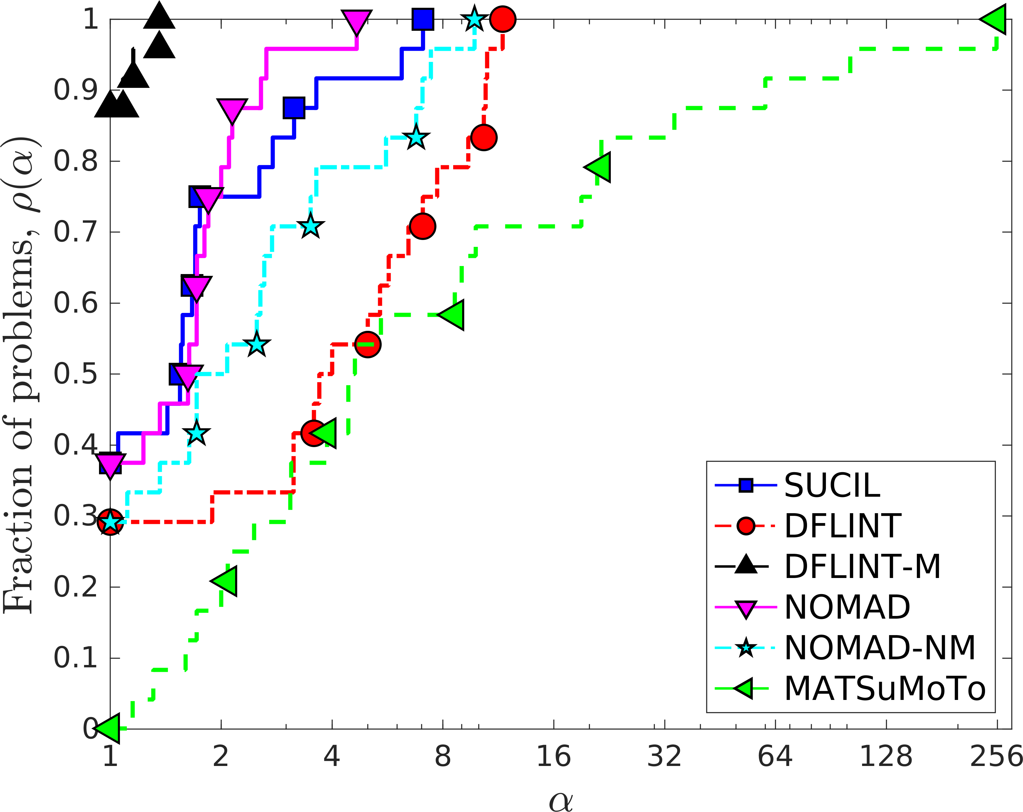
We now analyze the performance of SUCIL compared with the other methods. Figure 5 (left) shows the performance profiles for methods to terminate on the 24 test problems; Figure 5 (right) compares the number of function evaluations required before each method first evaluates a global minimizer. This comparison is nontrivial because each solver has its own design considerations and notions of local optimality. Also, the other solvers do not assume convexity of the problem or exploit it. Hence, our results merely demonstrate that SUCIL provably converges to a global optimum and uses fewer function evaluations because of its exploitation of convexity. Figure 5 shows that our algorithm requires the least number of function evaluations for more than 65% of the instances and provides a global optimality certificate, in addition. In reaching the global optimal solution quickly, however, DFLINT-M wins for more than 85% of the instances. Although SUCIL is not particularly designed to greedily descend to the global optimum, it is still competitive with the rest of the methods on this front.

7 Discussion

The order of results in this paper tells the story of how we arrived at the implementation of SUCIL. We first attempted to classify where linear interpolation models provide lower bounds for convex functions, yielding the results in Section 3; we then proved that such linear functions can underlie a convergent algorithm, as in Section 4. We initially modeled the secants and the conditions in which they are valid as an MILP, as in Section 5.1.1. After observing that the number of variables in the MILP model was larger than the number of points in the domain $\Omega$ , we were motivated to develop the enumerative model in Section 5.1.2.

Our computational developments expose a number of fundamental challenges for integer derivative-free optimization. The complexity of our piecewise linear model (PLP) is made worse by the fact that each secant function is valid only in the union of $n+1$ cones $\mathcal{U}^{\mbox{\boldmath$i$}}$ , resulting in conditional cuts. We note that it may not be possible to derive unconditional cuts, that is, cuts that are valid in the whole domain $\Omega$ . For example, we might initially consider secants interpolating a convex $f$ at the $n+1$ points $x\in\mathbb{Z}^{n}$ and $x\pm e_{i}\in\mathbb{Z}^{n}$ , where for every $i$ we can choose either $+$ or $-$ . Such points form a unit simplex that has no integer points in its interior. Consequently, one might suspect that the resulting cut is valid everywhere in $\Omega$ . However, the following example shows that the resulting cut is not unconditionally valid. Consider $f(x)=x_{1}^{2}-x_{1}x_{2}+x_{2}^{2}$ and the set of points $\{[1,1]^{\operatorname{T}},[0,1]^{\operatorname{T}},[1,0]^{\operatorname{T}}\}$ . It follows that $f(x)=1$ at these points, and hence the unique interpolating secant function is the constant function, $m(x)=1$ . Now consider the point $x=[0,0]^{\operatorname{T}}$ for which $f(x)=0$ , which is not underestimated by $m(x)=1$ . Another limitation of our method is that it will have to evaluate all feasible points when $\Omega=\{0,1\}^{n}$ (a pure binary domain) for convergence because no point in $\Omega\setminus X^{\mbox{\boldmath$i$}}$ belongs to $\mathcal{U}^{\mbox{\boldmath$i$}}$ , where $X^{\mbox{\boldmath$i$}}$ is an arbitrary poised set of $n+1$ points in $\{0,1\}^{n}$ .

In Figure 6 we show the number of function evaluations needed to first evaluate a global minimizer and the additional number of evaluations used to prove it is a global minimizer. As is common, the effort required to certify optimality can be significantly larger than the cost of finding the optimum. In terms of number of function evaluations required, the proof of optimality is even more time consuming. Because the iterations where $X^{k}$ or $G^{k}$ is large require checking many potential secant functions, in SUCIL the computational cost of iterations can differ by orders of magnitude as the algorithm progresses.

Although our method provides a practical iterative way to check sufficiency of a set of points (optimality conditions) for a given convex instance, each iteration involves construction and evaluation of a large number of combinations of different $n+1$ points, which limits the scalability of Algorithm 3 in solving instances of higher dimensions. Yet, in our numerical experiments, we observe that only a small fraction of the total cuts evaluated are useful. We call $(c^{\mbox{\boldmath$i$}},b^{\mbox{\boldmath$i$}})$ an updating cut at an iteration $k$ if there exists an $x\in\Omega_{k}$ such that $m^{\mbox{\boldmath$i$}}(x)>\eta_{k}(x)$ , that is, a cut that improves the lower bound at at least one $x\in\Omega_{k}$ . In addition, if $m^{\mbox{\boldmath$i$}}(x)\geq u_{k}$ , we call it a pruning cut. A pruning cut helps eliminate points to be considered in the next iteration ( $\Omega_{k+1}$ ). Figure 7 shows the number of updating and pruning cuts generated per iteration of SUCIL when minimizing quad on $[-4,4]^{3}\cap\mathbb{Z}^{3}$ . The fact that few cuts prune a point or update the lower bound at any point where the minimum could be suggests that there may be some way to exclude a large set of multi-indices from consideration, possibly yielding dramatic computational savings.

Ideally, we would like to evaluate only the combinations that yield updating or pruning cuts. However, this approach requires the solution of a separate problem that we believe is especially hard to solve. Even the following simpler problem of finding a pruning cut at a given candidate point seems difficult.

Problem 1.

Given a point $\bar{x}\in\mathbb{Z}^{n}$ , a set of (integer) points $X$ where $f$ has been evaluated, and scalar $u$ , find a cut that prunes $\bar{x}$ . That is, find a multi-index $i$ such that $\bar{x}\in\mathcal{U}^{\mbox{\boldmath$i$}}$ and ${(c^{\mbox{\boldmath$i$}})}^{\operatorname{T}}\bar{x}+b^{\mbox{\boldmath$i$}}\geq u$ , and $(c^{\mbox{\boldmath$i$}},b^{\mbox{\boldmath$i$}})$ solves (3), or show that no such multi-index $i$ exists.

If we choose a small subset $\bar{X^{k}}$ of $X^{k}$ to form $W(\bar{X}^{k})$ , the SUCIL algorithm can end up using a large number of function evaluations to obtain a certificate of optimality. The reason is that points are evaluated that would be ruled worse than optimal if secants were built by using all combinations of points in $X^{k}$ . This situation occurred when setting $\bar{X^{k}}$ to be a random subset of $X^{k}$ , a subset of the points closest to $\hat{x}$ , or a subset of points with best function values. Using $G^{k}$ avoids discarding too many points from $X^{k}$ ; but we observe a significant increase in $\left|W(G^{k})\right|$ , and thus we incur heavy computational costs during some iterations. The wall-clock time required per iteration for solving instances of dimension less than 5 in our setup is not significant, but we present the same for 5-dimensional instances using SUCIL on a 96-core Intel Xeon computer with 1.5 TB of RAM. The complexity of our approach is better quantified by counting the number of combinations of points (or potential secants) considered at iteration $k$ . Using $G^{k}$ , we typically produce a strict subset of all possible combinations in such a way that the size of $W(G^{k})$ decreases during the later iterations. This is shown in Figure 8: the number of secants added per iteration for all 5-dimensional test instances using SUCIL. Once $\Omega_{k}$ , the number of points with $\eta(x)$ less than $f(\hat{x})$ , starts decreasing, so do $G^{k}$ and $\left|W(G^{k})\right|$ . In general, it is difficult to predict when the number of combinations (or the wall-clock time curve) would be at the peak, but we suspect this peak will be worse as $n$ increases, by both the size and the iteration number where it occurs. This limits the applicability of the current implementation of SUCIL on higher-dimensional problems.

Again, since nearly all cuts in $W(G^{k})$ do not update $\eta(x)$ at any point in $\Omega_{k}$ (see Figure 7), we believe there may be some approach for intelligently selecting points from $X^{k}$ using their geometry, their function values, and distance from $\hat{x}$ that will rule some multi-indices $i$ as unnecessary to consider. We did attempt to identify minimal sets of points that were necessary for SUCIL to certify optimality for a variety of $n=2$ test cases, but no general rule was apparent.

We note that the storage requirements for the enumerative model may be prohibitive, even for moderate problem sizes. For example, an array storing the value of $\eta(x)$ as an 8-byte scalar for all $x\in\Omega=[-10,10]^{10}\cap\mathbb{Z}^{10}$ would require over 200 GB of storage.

Ultimately, we believe further insights are yet to be discovered that will facilitate better algorithms for minimizing convex functions on integer domains.

Acknowledgements

We are grateful to Eric Ni for his insights on derivative-free algorithms for unrelaxable integer variables. Sven Leyffer also wishes to acknowledge the insightful discussions on an early draft of this work during the Dagstuhl seminar 18081. This material is based upon work supported by the applied mathematics and SciDAC activities of the Office of Advanced Scientific Computing Research, Office of Science, U.S. Department of Energy, under Contract DE-AC02-06CH11357.

Appendix A Test Problems

Table A1: Set of convex test problems.

Name	Expression	$f(x^{*})$	$x^{*}$
CB3II [11]	$\displaystyle\max\left\{\sum_{i=1}^{n-1}x_{i}^{4}+x_{i+1}^{2},\sum_{i=1}^{n-1}\left(2-x_{i}\right)^{2}+\left(2-x_{i+1}\right)^{2},\sum_{i=1}^{n-1}2e^{-x_{i}+x_{i+1}}\right\}$	$2(n-1)$	$e$
CB3I [10]	$\displaystyle\sum_{i=1}^{n-1}\max\left\{x_{i}^{4}+x_{i+1}^{2},\left(2-x_{i}\right)^{2}+\left(2-x_{i+1}\right)^{2},2e^{-x_{i}+x_{i+1}}\right\}$	$2(n-1)$	$e$
KLT [29]	$\displaystyle\max_{i\in\left\{1,\ldots,n\right\}}\left\{\left\\|x-c_{i}-2e\right\\|^{2}\right\},c_{i}=2e_{i}-e$	$n$	$2e$
LQ [22]	$\displaystyle\sum_{i=1}^{n-1}\max\left\{-x_{i}-x_{i+1},-x_{i}-x_{i+1}+x^{2}_{i}+x^{2}_{i+1}-1\right\}$	$-(n-1)$	many
abhi [1]	$\displaystyle\sum_{i=1}^{n}\left[64\left(c_{1}(x_{i}-2)-c_{2}(x_{i+1}-2)\right)^{2}+\left(c_{2}(x_{i}-2)-c_{1}(x_{i+1}-2)\right)^{2}\right]$ , $c_{1}=\cos\left(\frac{\pi}{8}\right),c_{2}=\sin\left(\frac{\pi}{8}\right)$	0	$2e$
maxq [22]	$\displaystyle\max_{i\in\left\{1,\ldots,n\right\}}\left\{x^{2}_{i}\right\}$	0	0
mxhilb [28]	$\displaystyle\max_{i\in\left\{1,\ldots,n\right\}}\left\{\sum_{j=1}^{n}\left\lvert\frac{x_{j}}{i+j-1}\right\rvert\right\}$	0	0
quad	$\displaystyle\sum_{i=1}^{n}\left(x_{i}-2\right)^{2}$	0	$2e$

Appendix B Performance of MILP Model

Table B1: Characteristics of the first 12 instances of (CPF) generated by Algorithm 1 minimizing the convex quadratic function abhi on

\Omega=[-2,2]^{3}\cap\mathbb{Z}^{3}

. (CPF) instances are generated by AMPL and solved by CPLEX; times are the mean of five replications.

k	sHyp	LB	UB	time	simIter	nodes	bVars	cVars	cons	$\hat{x}$
1	20	-616.3	79.9	0.1	374	0	335	268	960	$[2;2;-2]$
2	52	-555.1	79.9	3.9	13,180	8,089	847	685	2,466	$[2;2;-1]$
3	100	-475.2	44.7	10.9	31,423	8,555	1,615	1,310	4,724	$[2;1;-2]$
4	172	-434.4	44.7	7.3	19,267	1,728	2,767	2,247	8,110	$[1;2;-2]$
5	276	-413.9	19.1	30.8	68,264	5,874	4,431	3,600	13,000	$[2;1;-1]$
6	418	-373.1	19.1	95.1	84,031	7,933	6,703	5,447	19,676	$[1;2;-1]$
7	611	-311.7	19.1	59.6	83,102	5,440	9,791	7,957	28,749	$[2;-2;-2]$
8	866	-293.2	19.1	99.6	86,318	3,933	13,871	11,273	40,736	$[1;1;-2]$
9	1,196	-232.0	19.1	154.2	84,440	4,568	19,151	15,564	56,248	$[1;1;-1]$
10	1,532	-199.5	19.1	452.3	235,473	6,400	24,527	19,933	72,042	$[2;-2;-1]$
11	2,038	-192.9	19.1	1,006	387,491	9,686	32,623	26,512	95,826	$[2;-1;-2]$
12	2,605	-140.9	19.1	964.3	455,939	29,279	41,695	33,884	122,477	$[1;-1;-2]$

Table B1 shows the size of the MILP model at each iteration and the computational effort required for solving it. The column k refers to the iteration of Algorithm 1, sHyp denotes the number of secants (i.e., $\left|W(X)\right|$ ), and LB and UB give the lower and upper bound on $f$ on $\Omega$ , respectively. We show the computational effort needed to solve each MILP via time, the mean solution time (in seconds) for $5$ replications; simIter, the number of simplex iterations; and nodes, the number of branch-and-bound nodes explored by the MILP solver. The size of each MILP (after presolve) is shown in terms of bVars, the number of binary variables; cVars, the number of continuous variables; and cons, the number of constraints. Table B1 also shows the optimal solution $\hat{x}$ of each MILP. These experiments were performed by using CPLEX (v.12.6.1.0) on a 2.20 GHz, 12-core Intel Xeon computer with 64 GB of RAM. For this small problem we see that the size of the MILP grows exponentially as the iterations proceed, which results in an exponential growth in solution time as illustrated in Figure 3. The iteration 13 MILP was not solved after $30$ minutes.

Appendix C Detailed Numerical Results

Tables C1–C6 contain detailed numerical results for the interested reader. Note that some solvers do not respect the given budget of function evaluations. We have used a different stopping criterion for MATSuMoTo: it is set to stop only when a point with the optimal value has been identified. Also, although the global minimum is the starting point for maxq and mxhilb, MATSuMoTo instead uses its initial symmetric Latin hypercube design. The last row of Table 1 in Section 2 shows $\left|\Omega\right|$ for these problems.

Table C1: Number of function evaluations before solvers terminate for

n=3

test problems. Parentheses show number of evaluations until

x^{*}

is evaluated.

	SUCIL-ideal1	SUCIL	DFLINT	DFLINT-M	NOMAD	NOMAD-dm	MATSuMoTo
abhi	19 (8)	30 (17)	161 (57)	150 (10)	59 (20)	129 (56)	60 (31)
quad	25 (8)	39 (17)	157 (54)	150 (10)	53 (18)	119 (35)	45 (16)
KLT	22 (8)	28 (13)	152 (48)	146 (15)	51 (24)	116 (34)	46 (17)
maxq	14 (1)	14 (1)	181 (1)	181 (1)	34 (1)	107 (1)	50 (21)
mxhilb	16 (1)	21 (1)	181 (1)	181 (1)	35 (1)	106 (1)	48 (19)
LQ	18 (8)	36 (7)	182 (7)	181 (7)	48 (7)	107 (7)	41 (12)
CB3I	22 (8)	25 (10)	184 (22)	181 (7)	56 (12)	108 (12)	60 (31)
CB3II	22 (8)	34 (11)	184 (22)	181 (7)	44 (12)	108 (12)	60 (31)

Table C2: Number of function evaluations before solvers terminate for

n=4

test problems. Parentheses show number of evaluations until

x^{*}

is evaluated.

	SUCIL-ideal1	SUCIL	DFLINT	DFLINT-M	NOMAD	NOMAD-dm	MATSuMoTo
abhi	45 (10)	75 (41)	993 (137)	959 (13)	110 (16)	453 (88)	89 (60)
quad	51 (10)	95 (21)	982 (124)	959 (13)	111 (12)	460 (89)	56 (25)
KLT	51 (10)	67 (21)	954 (141)	953 (20)	116 (42)	457 (55)	54 (23)
maxq	30 (1)	33 (1)	1,001 (1)	1,001 (1)	91 (1)	451 (1)	89 (60)
mxhilb	32 (1)	65 (1)	1,001 (1)	1,001 (1)	90 (1)	450 (1)	63 (34)
LQ	39 (10)	109 (15)	1,000 (17)	1,001 (9)	145 (9)	453 (10)	47 (18)
CB3I	50 (10)	58 (14)	1,001 (58)	1,001 (9)	149 (42)	456 (23)	126 (81)
CB3II	48 (10)	91 (14)	1,001 (50)	1,001 (19)	125 (30)	460 (35)	131 (76)

Table C3: Number of function evaluations before solvers terminate for

n=5

test problems. Parentheses show number of evaluations until

x^{*}

is evaluated.

	SUCIL-ideal1	SUCIL	DFLINT	DFLINT-M	NOMAD	NOMAD-dm	MATSuMoTo
abhi	105 (12)	154 (113)	1,001 (167)	1,000 (16)	301 (41)	1,000 (156)	214 (157)
quad	108 (12)	146 (58)	1,001 (186)	1,000 (16)	286 (26)	1,000 (58)	113 (62)
KLT	108 (12)	121 (69)	1,001 (193)	1,001 (25)	296 (43)	1,000 (176)	108 (77)
maxq	75 (1)	80 (1)	1,001 (1)	1,001 (1)	257 (1)	1,000 (1)	284 (255)
mxhilb	96 (1)	154 (1)	1,001 (1)	1,001 (1)	257 (1)	1,000 (1)	131 (102)
LQ	83 (12)	126 (17)	1,001 (44)	1,001 (11)	425 (15)	1,000 (15)	56 (27)
CB3I	114 (12)	155 (68)	1,001 (103)	1,001 (11)	417 (18)	1,000 (18)	266 (237)
CB3II	100 (12)	135 (66)	1,001 (130)	1,001 (26)	465 (69)	1,000 (54)	281 (224)

Table C4: Number of function evaluations taken by 20 replications of MATSuMoTo for each of the

8

convex test problems for

n=3

	abhi	quad	KLT	maxq	mxhilb	LQ	CB3I	CB3II
1	48 (19)	48 (19)	48 (19)	43 (14)	48 (19)	43 (14)	59 (30)	83 (54)
2	63 (34)	44 (15)	44 (15)	48 (19)	44 (15)	43 (14)	43 (14)	54 (25)
3	44 (15)	43 (14)	45 (16)	48 (19)	49 (20)	43 (14)	48 (19)	106(77)
4	58 (29)	43 (14)	48 (19)	53 (24)	64 (35)	39 (10)	48 (19)	63 (34)
5	79 (50)	48 (19)	49 (20)	54 (25)	44 (15)	38 (9)	53 (24)	53 (24)
6	73 (44)	37 (9)	48 (19)	39 (10)	53 (24)	39 (10)	64 (35)	53 (24)
7	88 (59)	43 (14)	44 (15)	58 (29)	49 (20)	44 (15)	54 (25)	59 (30)
8	60 (31)	48 (19)	43 (14)	38 (9)	43 (14)	44 (15)	73 (44)	73 (44)
9	79 (50)	43 (14)	48 (19)	53 (24)	43 (14)	39 (10)	68 (39)	58 (29)
10	65 (36)	53 (24)	49 (20)	53 (24)	49 (20)	44 (15)	49 (20)	43 (14)
11	63 (34)	48 (19)	48 (19)	48 (19)	58 (29)	43 (14)	63 (34)	48 (19)
12	53 (24)	44 (15)	43 (14)	48 (19)	48 (19)	38 (9)	58 (29)	53 (24)
13	48 (19)	49 (20)	48 (19)	54 (25)	49 (20)	53 (24)	68 (39)	37 (9)
14	43 (14)	48 (19)	48 (19)	43 (14)	49 (20)	43 (14)	78 (49)	49 (20)
15	44 (15)	48 (19)	48 (19)	48 (19)	48 (19)	43 (14)	39 (10)	73 (44)
16	58 (29)	48 (19)	43 (14)	58 (29)	37 (9)	38 (9)	58 (29)	73 (44)
17	48 (19)	44 (15)	43 (14)	53 (24)	49 (20)	37 (9)	68 (39)	48 (19)
18	64 (35)	43 (14)	48 (19)	63 (34)	53 (24)	38 (9)	93 (64)	69 (40)
19	74 (45)	43 (14)	48 (19)	58 (29)	53 (24)	37 (9)	68 (39)	63 (34)
20	49 (20)	43 (14)	43 (14)	58 (29)	48 (19)	44 (15)	54 (25)	58 (29)
$\lfloor\mathbf{\rm mean}\rfloor$	60 (31)	45 (16)	46 (17)	50 (21)	48 (19)	41 (12)	60 (31)	60 (31)

Table C5: Number of function evaluations taken by 20 replications of MATSuMoTo for each of the

8

convex test problems for

n=4

	abhi	quad	KLT	maxq	mxhilb	LQ	CB3I	CB3II
1	110 (81)	56 (27)	51 (22)	66 (37)	60 (31)	41 (12)	230 (20)	85 (56)
2	70 (41)	55 (26)	60 (31)	120 (91)	60 (31)	46 (17)	76 (47)	85 (56)
3	50 (21)	50 (21)	50 (21)	94 (65)	50 (21)	41 (12)	150 (121)	196 (11)
4	104 (75)	50 (21)	50 (21)	65 (36)	80 (51)	45 (16)	110 (81)	186 (16)
5	91 (62)	60 (11)	55 (26)	112 (83)	80 (51)	41 (12)	100 (11)	161 (132)
6	66 (37)	55 (26)	56 (27)	90 (61)	56 (27)	55 (26)	101 (72)	196 (167)
7	86 (57)	65 (36)	45 (16)	65 (36)	50 (21)	46 (17)	90 (61)	141 (112)
8	90 (61)	55 (26)	65 (11)	81 (52)	65 (36)	41 (12)	105 (63)	346 (161)
9	166 (137)	56 (27)	56 (27)	55 (26)	50 (21)	51 (22)	96 (67)	100 (71)
10	85 (56)	65 (21)	55 (11)	60 (31)	65 (36)	55 (26)	55 (26)	106 (77)
11	147 (118)	70 (41)	46 (17)	70 (41)	65 (36)	46 (17)	95 (66)	80 (51)
12	96 (67)	45 (16)	46 (17)	112 (83)	71 (42)	50 (21)	112 (83)	231 (202)
13	39 (11)	60 (31)	71 (42)	119 (90)	71 (42)	41 (12)	50 (21)	81 (52)
14	85 (56)	61 (32)	50 (21)	85 (56)	55 (26)	55 (26)	205 (176)	55 (26)
15	101 (72)	60 (31)	60 (31)	94 (65)	55 (26)	41 (12)	160 (131)	114 (85)
16	66 (37)	51 (22)	45 (16)	50 (21)	75 (46)	41 (12)	65 (36)	65 (36)
17	76 (47)	65 (36)	56 (27)	55 (26)	60 (31)	60 (31)	85 (56)	131 (102)
18	70 (41)	56 (27)	51 (22)	110 (81)	75 (46)	65 (36)	314 (285)	70 (41)
19	81 (52)	56 (11)	60 (31)	221 (192)	71 (42)	41 (12)	117 (16)	141 (52)
20	105 (76)	46 (17)	60 (31)	66 (37)	50 (21)	56 (27)	210 (13)	50 (21)
$\lfloor\mathbf{\rm mean}\rfloor$	89 (60)	56 (25)	54 (23)	89 (60)	63 (34)	47 (18)	126 (81)	131 (76)

Table C6: Number of function evaluations taken by 20 replications of MATSuMoTo for each of the

8

convex test problems for

n=5

	abhi	quad	KLT	maxq	mxhilb	LQ	CB3I	CB3II
1	472 (443)	82 (53)	83 (54)	137 (108)	149 (120)	52 (23)	199 (170)	83 (54)
2	358 (329)	83 (54)	317 (288)	229 (200)	208 (179)	63 (34)	267 (238)	518 (489)
3	193 (164)	83 (54)	172 (143)	115 (86)	175 (146)	62 (33)	377 (348)	1,626 (133)
4	194 (165)	73 (44)	62 (33)	171 (142)	72 (43)	57 (28)	223 (194)	325 (296)
5	160 (131)	72 (43)	73 (44)	504 (475)	87 (58)	53 (24)	835 (806)	487 (458)
6	396 (367)	187 (127)	78 (49)	92 (63)	152 (123)	53 (24)	127 (98)	196 (18)
7	82 (53)	82 (53)	120 (91)	135 (106)	247 (218)	62 (33)	184 (155)	603 (574)
8	62 (33)	106 (15)	58 (29)	969 (940)	186 (157)	52 (23)	164 (135)	67 (38)
9	107 (78)	83 (54)	68 (39)	276 (247)	103 (74)	57 (28)	399 (370)	671 (642)
10	186 (13)	78 (18)	73 (44)	352 (323)	82 (53)	73 (44)	364 (335)	205 (18)
11	181 (152)	130 (65)	62 (33)	255 (226)	53 (24)	58 (29)	414 (385)	240 (211)
12	239 (210)	115 (86)	125 (96)	403 (374)	181 (152)	47 (18)	83 (54)	462 (433)
13	295 (211)	87 (18)	72 (43)	167 (138)	151 (122)	48 (19)	128 (99)	324 (33)
14	354 (325)	78 (49)	72 (43)	236 (207)	82 (53)	62 (33)	200 (171)	154 (125)
15	113 (13)	73 (44)	52 (14)	512 (483)	88 (59)	53 (24)	271 (242)	87 (58)
16	227 (23)	82 (53)	120 (91)	189 (160)	93 (64)	68 (39)	326 (297)	63 (34)
17	102 (73)	135 (106)	270 (241)	195 (166)	57 (28)	58 (29)	180 (151)	599 (570)
18	139 (110)	268 (80)	150 (121)	173 (144)	112 (83)	58 (29)	228 (199)	112 (83)
19	169 (19)	67 (38)	72 (43)	108 (79)	117 (88)	42 (13)	204 (175)	93 (64)
20	268 (239)	301 (195)	62 (13)	465 (436)	237 (208)	53 (24)	162 (133)	180 (151)
$\lfloor\mathbf{\rm mean}\rfloor$	214 (157)	113 (62)	108 (77)	284 (255)	131 (102)	56 (27)	266 (237)	281 (224)

Appendix D Derivation of Tolerances

In this section, we show how one can compute sufficient values of $M_{\eta}$ , $\epsilon_{\lambda}$ , and $M_{\lambda}$ for the MILP model (CPF). We first show that if we choose these parameters incorrectly, then the resulting MILP model no longer provides a valid lower bound.

Effect of an Insufficient $\epsilon_{\lambda}$ Value.

A large $\epsilon_{\lambda}$ or small $M_{\lambda}$ (or both) could result in an incorrect value of $z^{i_{j}}=1$ for a point $x\notin\mathrm{cone}\big(x^{i_{j}}-X^{\mbox{\boldmath$i$}}\big)$ , violating the implication of $z^{i_{j}}=1$ and yielding an invalid lower bound on $f$ . This is illustrated using a one-dimensional example in Figure D1. Similarly, one can encounter an invalid lower bound at an iteration if $M_{\lambda}$ is chosen to be smaller than required.

Figure D1: An example of false termination of Algorithm 1 using (CPF) when an insufficient value of

\epsilon_{\lambda}

is used:

f(x)=x^{2}

and interpolation points

-1

and

1

are used to form the secant shown in red colour. Any value of

\epsilon_{\lambda}>0.5

forces

z^{{1}_{1}}=z^{{1}_{2}}=1

, activating the cut

\eta\geq 1

at the optimal

x^{*}=0

, resulting in

l_{f}^{k}=u_{f}^{k}=1

Bound on $M_{\eta}$

Let $l_{f}$ be a valid lower bound of $f$ on $\Omega$ . With this lower bound, scalars $M_{\mbox{\boldmath$i$}}$ can be defined as

M_{\mbox{\boldmath$i$}}=\max\limits_{x\in\Omega}\{(c^{\mbox{\boldmath$i$}})^{T}x+b^{\mbox{\boldmath$i$}}\}-l_{f},\;\forall\mbox{\boldmath$i$}\in W(X).

(26)

If $\Omega=\left\{x:l_{x}\leq x\leq u_{x}\right\}$ , where $l_{x},u_{x}\in\mathbb{R}^{n}$ are known, then we can set

M_{\mbox{\boldmath$i$}}=\sum_{h:c^{\mbox{\boldmath$i$}}_{j}<0}c^{\mbox{\boldmath$i$}}_{h}l_{x}+\sum_{h:c^{\mbox{\boldmath$i$}}_{j}\geq 0}c^{\mbox{\boldmath$i$}}_{h}u_{x}+b^{\mbox{\boldmath$i$}}-l_{f},\quad h=1,\ldots,n,\;\forall\mbox{\boldmath$i$}\in W(X).

(27)

Then, we can either set individual values of $M_{\mbox{\boldmath$i$}}$ within each constraint (15), which would yield a tighter model, or use a single parameter,

M_{\eta}=\max\limits_{\mbox{\boldmath$i$}}\{M_{\mbox{\boldmath$i$}}\},

(28)

as shown in (CPF).

Bounds on $\epsilon_{\lambda}$ and $M_{\lambda}$

Sufficient values of $M_{\lambda}$ and $\epsilon_{\lambda}$ are not easy to calculate as they depend on the rays generated at $x^{i_{j}}$ , and the domain $\Omega$ . We show next, that bounds on these values can be computed by solving a set of optimization problems. A sufficient value for $\epsilon_{\lambda}$ can be computed based on the representations of the $n+1$ hyperplanes formed using different combinations of $n$ points, $\forall\mbox{\boldmath$i$}\in W(X)$ . We can use one of the representations of the hyperplane passing through points $X^{i}\setminus\{x^{i_{j}}\},j=1\ldots n+1$ to obtain bounds on $\epsilon_{\lambda}$ , by solving an optimization problem for each $i_{j}\in\mbox{\boldmath$i$}$ . Let $c^{\mbox{\boldmath$i$}_{i_{j}-}}$ and $b^{\mbox{\boldmath$i$}_{i_{j}-}}$ denote the solution of the following problem.

$\displaystyle\displaystyle\mathop{\mbox{minimize}}_{c,b}$	$\displaystyle\left\\|c\right\\|_{1}$	(P $-hyp$ )
$\displaystyle\mbox{subject to }$	$\displaystyle\displaystyle(c)^{T}x^{i_{l}}+b=0,\quad l=1,\ldots,n+1,\;l\neq j$
	$\displaystyle\displaystyle\left\\|c\right\\|_{1}\geq 1$
	$\displaystyle\displaystyle c\in\mathbb{Z}^{n},b\in\mathbb{Z}.$

Problem (P - ⁢ h y p ) can be easily cast as an integer program by replacing $\left\|c\right\|_{1}$ by $e^{T}y$ , where $e=(1,\ldots,1)^{T}$ is the vector or all ones, and the variables $y$ satisfy the constraints $y\geq c,y\geq-c$ . Because, the hyperplane is generated using $n$ integer points, it can be shown that there exists a solution $c^{\mbox{\boldmath$i$}_{i_{j}-}}$ and $b^{\mbox{\boldmath$i$}_{i_{j}-}}$ that is nonzero and integral, as stated in the following proposition.

Proposition D.1.

Consider a hyperplane $S=\{x:c^{T}x+b=0\}$ such that $c$ and $b$ are integral. The Euclidean distance between an arbitrary point $\hat{x}\in\mathbb{Z}^{n}\setminus S$ , and $S$ , is greater than or equal to $\frac{1}{\lvert\lvert c\rvert\rvert_{2}}$ .

Proof.

The Euclidean distance between a point $\hat{x}$ and $S$ is the 2-norm of the projection of the line segment joining an arbitrary point $w\in S$ and $\hat{x}$ , on the normal passing through $\hat{x}$ , and can be expressed as

\frac{\lvert c^{T}\hat{x}+b\rvert}{\lvert\lvert c\rvert\rvert_{2}}.

(29)

By integrality of $c,b$ and $\hat{x}$ , and since $\hat{x}\notin S$ , $\lvert c^{T}\hat{x}+b\rvert\geq 1$ , and the result follows. ∎∎

Proposition D.1 can be used directly to get a sufficient value of $\epsilon_{\lambda}$ as follows.

\epsilon_{\lambda}=\min\limits_{\mbox{\boldmath$i$}\in W(X),\;i_{j}\in\mbox{\boldmath$i$}}{\;\frac{1}{\lvert\lvert c^{\mbox{\boldmath$i$}_{i_{j}-}}\rvert\rvert_{2}}}.

(30)

The bound can be tightened using the following optimization problem.

$\displaystyle\displaystyle\mathop{\mbox{minimize}}_{x}$	$\displaystyle\frac{\lvert(c^{\mbox{\boldmath$i$}_{i_{j}-}})^{T}x+b^{\mbox{\boldmath$i$}_{i_{j}-}}\rvert}{\lvert\lvert c^{\mbox{\boldmath$i$}_{i_{j}-}}\rvert\rvert_{2}}$	(P- $\epsilon$ )
$\displaystyle\mbox{subject to }$	$\displaystyle\displaystyle\lvert(c^{\mbox{\boldmath$i$}_{i_{j}-}})^{T}x^{i_{l}}+b^{\mbox{\boldmath$i$}_{i_{j}-}}\rvert\geq 1$
	$\displaystyle\displaystyle x\in\Omega.$

If we denote by $\epsilon^{\mbox{\boldmath$i$}_{i_{j}-}}_{\lambda}$ , the optimal value of (P- ϵ ), then the following is a sufficient value of $\epsilon_{\lambda}$ .

\epsilon_{\lambda}=\min\limits_{\mbox{\boldmath$i$}\in W(X),\;i_{j}\in\mbox{\boldmath$i$}}{\;\epsilon_{\lambda}^{\mbox{\boldmath$i$}_{i_{j}-}}}.

(31)

Similarly, if we maximize the objective in (P- ϵ ), and denote the optimal value by $M^{\mbox{\boldmath$i$}_{i_{j}-}}_{\lambda}$ we get a sufficient value for $M_{\lambda}$ as follows.

M_{\lambda}=\max\limits_{\mbox{\boldmath$i$}\in W(X),\;i_{j}\in\mbox{\boldmath$i$}}{\;M_{\lambda}^{\mbox{\boldmath$i$}_{i_{j}-}}}.

(32)

No-Good Cuts and Stronger Objective Bounds.

For our initial experiments, we tried setting arbitrarily small values for $\epsilon_{\lambda}$ instead of obtaining the best possible values by solving a set of optimization problems as elaborated above. The problem with having such values of $\epsilon_{\lambda}>0$ too small is that it allows us to ignore the cuts at the interpolation points, $x^{(k)}$ , causing a violation of the bound, $\eta\geq f^{(k)}$ , for $x=x^{(k)}$ in the MILP, resulting in repetition of iterates in the algorithm. We fixed this by adding the following valid inequality to the MILP.

\eta\geq f^{(k)}-M\|x^{(k)}-x\|_{1}.

We can write this inequality as a linear constraint, by introducing a binary representation of the variables, $x$ , requiring $nU$ binary variables, $\xi_{ij},\;i=1,\ldots,n,\;j=1,\ldots,U$ , where $n$ is the dimension of our problem, and $0\leq x\leq U$ . With this representation, we obtain

x_{i}=\sum_{j=1}^{U}i\xi_{ij},\quad 1=\sum_{j=1}^{U}\xi_{ij},\quad\xi_{ij}\in\{0,1\},

and write the $\eta$ -constraint equivalently as

\eta\geq f^{(k)}-M\sum_{i=1}^{n}\left(\sum_{j:\xi_{ij}^{(k)}=0}\xi_{ij}+\sum_{j:\xi_{ij}^{(k)}=1}\left(1-\xi_{ij}\right)\right).

References

[1] Abhishek, K., Leyffer, S., Linderoth, J.T.: Modeling without categorical variables: A mixed-integer nonlinear program for the optimization of thermal insulation systems. Optimization and Engineering 11(2), 185–212 (2010). DOI 10.1007/s11081-010-9109-z
[2] Abramson, M., Audet, C., Chrissis, J., Walston, J.: Mesh adaptive direct search algorithms for mixed variable optimization. Optimization Letters 3(1), 35–47 (2009). DOI 10.1007/s11590-008-0089-2
[3] Abramson, M.A., Audet, C., Couture, G., Dennis Jr, J.E., Le Digabel, S., Tribes, C.: The NOMAD project (2014). URL https://www.gerad.ca/nomad
[4] Audet, C., Dennis, Jr., J.E.: Pattern search algorithms for mixed variable programming. SIAM Journal on Optimization 11(3), 573–594 (2000). DOI 10.1137/S1052623499352024
[5] Audet, C., Le Digabel, S., Tribes, C.: The mesh adaptive direct search algorithm for granular and discrete variables. Tech. Rep. 6526, Optimization Online (2018). URL http://www.optimization-online.org/DB_HTML/2018/03/6526.html
[6] Balaprakash, P., Tiwari, A., Wild, S.M.: Multi-objective optimization of HPC kernels for performance, power, and energy. In: S.A. Jarvis, S.A. Wright, S.D. Hammond (eds.) High Performance Computing Systems. Performance Modeling, Benchmarking and Simulation, vol. 8551, pp. 239–260. Springer (2014). DOI 10.1007/978-3-319-10214-6˙12
[7] Bartz-Beielstein, T., Zaefferer, M.: Model-based methods for continuous and discrete global optimization. Applied Soft Computing 55, 154–167 (2017). DOI 10.1016/j.asoc.2017.01.039
[8] Bonami, P., Biegler, L., Conn, A., Cornuéjols, G., Grossmann, I., Laird, C., Lee, J., Lodi, A., Margot, F., Sawaya, N., Wächter, A.: An algorithmic framework for convex mixed integer nonlinear programs. Discrete Optimization 5(2), 186–204 (2008). DOI 10.1016/j.disopt.2006.10.011
[9] Buchheim, C., Kuhlmann, R., Meyer, C.: Combinatorial optimal control of semilinear elliptic PDEs. Computational Optimization and Applications 70(3), 641–675 (2018). DOI 10.1007/s10589-018-9993-2
[10] Charalambous, C., Bandler, J.W.: Non-linear minimax optimization as a sequence of least $p$ th optimization with finite values of $p$ . International Journal of Systems Science 7(4), 377–391 (1976). DOI 10.1080/00207727608941924
[11] Charalambous, C., Conn, A.R.: An efficient method to solve the minimax problem directly. SIAM Journal on Numerical Analysis 15(1), 162–187 (1978). DOI 10.1137/0715011
[12] Conn, A.R., Scheinberg, K., Vicente, L.N.: Introduction to Derivative-Free Optimization. MPS/SIAM Series on Optimization. Society for Industrial and Applied Mathematics (2009)
[13] Costa, A., Nannicini, G.: RBFOpt: An open-source library for black-box optimization with costly function evaluations. Mathematical Programming Computation 10(4), 597–629 (2018)
[14] Davis, E., Ierapetritou, M.: A kriging based method for the solution of mixed-integer nonlinear programs containing black-box functions. Journal of Global Optimization 43(2-3), 191–205 (2009). DOI 10.1007/s10898-007-9217-2
[15] Dennis, Jr., J.E., Woods, D.J.: Optimization on microcomputers: The Nelder-Mead simplex algorithm. In: A. Wouk (ed.) New Computing Environments: Microcomputers in Large-Scale Computing, pp. 116–122. SIAM (1987)
[16] Dolan, E.D., Moré, J.: Benchmarking optimization software with performance profiles. Mathematical Programming 91(2), 201–213 (2002). DOI 10.1007/s101070100263
[17] Duran, M.A., Grossmann, I.E.: An outer-approximation algorithm for a class of mixed-integer nonlinear programs. Mathematical Programming 36(3), 307–339 (1986). DOI 10.1007/bf02592064
[18] Fletcher, R., Leyffer, S.: Solving mixed integer nonlinear programs by outer approximation. Mathematical Programming 66(1-3), 327–349 (1994). DOI 10.1007/bf01581153
[19] García-Palomares, U.M., Rodríguez-Hernández, P.S.: Unified approach for solving box-constrained models with continuous or discrete variables by non monotone direct search methods. Optimization Letters 13(1), 95–111 (2019). DOI 10.1007/s11590-018-1253-y
[20] Geoffrion, A.M., Marsten, R.E.: Integer programming algorithms: A framework and state-of-the-art survey. Management Science 18(9), 465–491 (1972). DOI 10.1287/mnsc.18.9.465
[21] Graf, P.A., Billups, S.: MDTri: Robust and efficient global mixed integer search of spaces of multiple ternary alloys. Computational Optimization and Applications 68(3), 671–687 (2017). DOI 10.1007/s10589-017-9922-9
[22] Haarala, M., Miettinen, K., Mäkelä, M.M.: New limited memory bundle method for large-scale nonsmooth optimization. Optimization Methods and Software 19(6), 673–692 (2004). DOI 10.1080/10556780410001689225
[23] Hemker, T., Fowler, K., Farthing, M., von Stryk, O.: A mixed-integer simulation-based optimization approach with surrogate functions in water resources management. Optimization and Engineering 9(4), 341–360 (2008). DOI 10.1007/s11081-008-9048-0
[24] Hemmecke, R., Köppe, M., Lee, J., Weismantel, R.: Nonlinear integer programming. In: 50 Years of Integer Programming 1958–2008, pp. 561–618. Springer (2010). DOI 10.1007/978-3-540-68279-0˙15
[25] Holmström, K., Quttineh, N.H., Edvall, M.: An adaptive radial basis algorithm (ARBF) for expensive black-box mixed-integer constrained global optimization. Optimization and Engineering 9(4), 311–339 (2008). DOI 10.1007/s11081-008-9037-3
[26] Jian, N., Henderson, S.G.: Estimating the probability that a function observed with noise is convex. INFORMS Journal on Computing (2019). DOI 10.1287/ijoc.2018.0847
[27] Jian, N., Henderson, S.G., Hunter, S.R.: Sequential detection of convexity from noisy function evaluations. In: Proceedings of the Winter Simulation Conference. IEEE (2014). DOI 10.1109/wsc.2014.7020215
[28] Kiwiel, K.C.: An ellipsoid trust region bundle method for nonsmooth convex minimization. SIAM Journal on Control and Optimization 27(4), 737–757 (1989). DOI 10.1137/0327039
[29] Kolda, T.G., Lewis, R.M., Torczon, V.J.: Optimization by direct search: New perspectives on some classical and modern methods. SIAM Review 45(3), 385–482 (2003). DOI 10.1137/S003614450242889
[30] Le Digabel, S., Wild, S.M.: A taxonomy of constraints in black-box simulation-based optimization. Preprint ANL/MCS-P5350-0515, Argonne (2015-01). URL http://www.mcs.anl.gov/papers/P5350-0515.pdf
[31] Liuzzi, G., Lucidi, S., Rinaldi, F.: Derivative-free methods for bound constrained mixed-integer optimization. Computational Optimization and Applications 53(2), 505–526 (2011). DOI 10.1007/s10589-011-9405-3
[32] Liuzzi, G., Lucidi, S., Rinaldi, F.: Derivative-free methods for mixed-integer constrained optimization problems. Journal of Optimization Theory and Applications 164(3), 933–965 (2015). DOI 10.1007/s10957-014-0617-4
[33] Liuzzi, G., Lucidi, S., Rinaldi, F.: An algorithmic framework based on primitive directions and nonmonotone line searches for black box problems with integer variables. Tech. Rep. 6471, Optimization Online (2018). URL http://www.optimization-online.org/DB_HTML/2018/02/6471.html
[34] Müller, J.: MATSuMoTo: The MATLAB surrogate model toolbox for computationally expensive black-box global optimization problems. Tech. Rep. 1404.4261, arXiv (2014). URL https://arxiv.org/abs/1404.4261
[35] Müller, J.: MISO: Mixed-integer surrogate optimization framework. Optimization and Engineering 17(1), 177–203 (2016). DOI 10.1007/s11081-015-9281-2
[36] Müller, J., Shoemaker, C.A., Piché, R.: SO-I: A surrogate model algorithm for expensive nonlinear integer programming problems including global optimization applications. Journal of Global Optimization 59(4), 865–889 (2013). DOI 10.1007/s10898-013-0101-y
[37] Müller, J., Shoemaker, C.A., Piché, R.: SO-MI: A surrogate model algorithm for computationally expensive nonlinear mixed-integer black-box global optimization problems. Computers & Operations Research 40(5), 1383–1400 (2013). DOI 10.1016/j.cor.2012.08.022
[38] Newby, E., Ali, M.M.: A trust-region-based derivative free algorithm for mixed integer programming. Computational Optimization and Applications 60(1), 199–229 (2015). DOI 10.1007/s10589-014-9660-1
[39] Porcelli, M., Toint, P.L.: BFO, a trainable derivative-free brute force optimizer for nonlinear bound-constrained optimization and equilibrium computations with continuous and discrete variables. ACM Transactions on Mathematical Software 44(1), 1–25 (2017). DOI 10.1145/3085592
[40] Rashid, K., Ambani, S., Cetinkaya, E.: An adaptive multiquadric radial basis function method for expensive black-box mixed-integer nonlinear constrained optimization. Engineering Optimization 45(2), 185–206 (2012). DOI 10.1080/0305215X.2012.665450
[41] Richter, P., Ábrahám, E., Morin, G.: Optimisation of concentrating solar thermal power plants with neural networks. In: A. Dobnikar, U. Lotrič, B. Šter (eds.) Adaptive and Natural Computing Algorithms, vol. 6593, pp. 190–199. Springer (2011). DOI 10.1007/978-3-642-20282-7˙20

The submitted manuscript has been created by UChicago Argonne, LLC, Operator of Argonne National Laboratory (“Argonne”). Argonne, a U.S. Department of Energy Office of Science laboratory, is operated under Contract No. DE-AC02-06CH11357. The U.S. Government retains for itself, and others acting on its behalf, a paid-up nonexclusive, irrevocable worldwide license in said article to reproduce, prepare derivative works, distribute copies to the public, and perform publicly and display publicly, by or on behalf of the Government. The Department of Energy will provide public access to these results of federally sponsored research in accordance with the DOE Public Access Plan. http://energy.gov/downloads/doe-public-access-plan

	$n=2$		$n=3$		$n=4$		$n=5$
$k$	$\lvert\Omega\rvert$	$\#$	$\lvert\Omega\rvert$	$\#$	$\lvert\Omega\rvert$	$\#$	$\lvert\Omega\rvert$	$\#$
1	9	8	27	26	81	80	243	242
2	25	16	125	98	625	544	3,125	2,882
3	49	32	343	290	2,403	2,240	16,807	16,322
4	81	48	729	578	6,561	5,856	59,049	55,682

A Method for Convex Black-Box Integer Global Optimization

Abstract

1 Introduction

Definition 1 (Convexity on Integer Subsets).

Assumption 1.

Outline.

2 Background

3 Underestimator of Convex Functions on the Integer Lattice

3.1 Secant Functions and Conditional Cuts

Definition 2.

Lemma 1 (Conditional Cuts).

Proof.

Lemma 2 (A Point Is In At Most One Cone).

Proof.

3.2 Lower Bound for ff

Lemma 3 (Underestimator of ff).

Proof.

3.3 Covering ℝn\mathbb{R}^{n} with Conditional Cuts

Lemma 4 (Poisedness of Initial Points).

Proof.

Lemma 5 (Initial Points and Coverage of Ω\Omega).

Proof.

4 Convergence Analysis

Theorem 1 (Convergence of Algorithm 1).

Proof.

5 Implementation Details

5.1 Formulating (PLP)

5.1.1 MILP Approach

5.1.2 Enumerative Approach

5.2 Other Implementation Details

5.2.1 Checking Whether X𝒊X^{\mbox{\boldmath$i$}} Is Poised and Whether x∈𝒰𝒊x\in\mathcal{U}^{\mbox{\boldmath$i$}}

Lemma 6 (Set Equality).

Proof.

5.2.2 Approximating W⁡(Xk∪{xk+1})W(X^{k}\cup\{x^{k+1}\})

Definition 3.

5.2.3 Selecting xk+1x^{k+1}

5.3 The SUCIL Method

Theorem 2 (Convergence of Algorithm 3).

Proof.

6 Numerical Experiments

7 Discussion

Problem 1.

Acknowledgements

Appendix A Test Problems

Appendix B Performance of MILP Model

Appendix C Detailed Numerical Results

Appendix D Derivation of Tolerances

Effect of an Insufficient ϵλ\epsilon_{\lambda} Value.

Bound on MηM_{\eta}

Bounds on ϵλ\epsilon_{\lambda} and MλM_{\lambda}

Proposition D.1.

Proof.

No-Good Cuts and Stronger Objective Bounds.

References

3.2 Lower Bound for $f$

Lemma 3 (Underestimator of $f$ ).

3.3 Covering $\mathbb{R}^{n}$ with Conditional Cuts

Lemma 5 (Initial Points and Coverage of $\Omega$ ).

5.2.1 Checking Whether $X^{\mbox{\boldmath$i$}}$ Is Poised and Whether $x\in\mathcal{U}^{\mbox{\boldmath$i$}}$

5.2.2 Approximating $W(X^{k}\cup\{x^{k+1}\})$

5.2.3 Selecting $x^{k+1}$

Effect of an Insufficient $\epsilon_{\lambda}$ Value.

Bound on $M_{\eta}$

Bounds on $\epsilon_{\lambda}$ and $M_{\lambda}$