Optimize TSK Fuzzy Systems for Regression Problems: Mini-Batch Gradient Descent with Regularization, DropRule, and AdaBound (MBGD-RDA)
Abstract
Takagi-Sugeno-Kang (TSK) fuzzy systems are very useful machine learning models for regression problems. However, to our knowledge, there has not existed an efficient and effective training algorithm that ensures their generalization performance, and also enables them to deal with big data. Inspired by the connections between TSK fuzzy systems and neural networks, we extend three powerful neural network optimization techniques, i.e., mini-batch gradient descent (MBGD), regularization, and AdaBound, to TSK fuzzy systems, and also propose three novel techniques (DropRule, DropMF, and DropMembership) specifically for training TSK fuzzy systems. Our final algorithm, MBGD with regularization, DropRule and AdaBound (MBGD-RDA), can achieve fast convergence in training TSK fuzzy systems, and also superior generalization performance in testing. It can be used for training TSK fuzzy systems on datasets of any size; however, it is particularly useful for big datasets, on which currently no other efficient training algorithms exist.
Index Terms:
Fuzzy systems, ANFIS, mini-batch gradient descent, regularization, AdaBound, DropRuleI Introduction
Fuzzy systems [1], particularly Takagi-Sugeno-Kang (TSK) fuzzy systems [2], have achieved great success in numerous applications. This paper focuses on the applications of TSK fuzzy systems in machine learning [3], particularly, supervised regression problems. In such problems, we have a training dataset with labeled examples , where , and would like to train a TSK fuzzy system to model the relationship between and , so that an accurate prediction can be made for any future unseen .
There are generally three different strategies for optimizing a TSK fuzzy system in supervised regression11 1 Some novel approaches for optimizing evolving fuzzy systems have also been proposed recently [4, 5]; however, they are not the focus of this paper, so their details are not included.:
- 1.
Evolutionary algorithms [6], in which each set of the parameters of the antecedent membership functions (MFs) and the consequents are encoded as an individual in a population, and genetic operators, such as selection, crossover, mutation, and reproduction, are used to produce the next generation. Generally, the overall fitness improves in each new generation, and a global optimum may be found given enough number of generations.
- 2.
- 3.
GD and least squares estimation (LSE) [10], which is used in the popular adaptive-network-based fuzzy inference system (ANFIS). The antecedent parameters are optimized by GD, and the consequent parameters by LSE. This approach usually converges much faster than using GD only.
However, all three strategies may have challenges in big data applications [11, 12]. It’s well-known that big data has at least three Vs22 2 There may be also other Vs, e.g., veracity, value, etc. [13]: volume (the size of the data), velocity (the speed of the data), and variety (the types of data). Volume means that the number of training examples () is very large, and/or the dimensionality of the input () is very high. Fuzzy systems, and actually almost all machine learning models, suffer from the curse of dimensionality, i.e., the number of rules (parameters) increases exponentially with . However, in this paper we assume that the dimensionality can be reduced effectively to just a few, e.g., using principal component analysis [14]. We mainly consider how to deal with large .
Evolutionary algorithms are not suitable for optimizing TSK fuzzy systems when is large, because they have very high memory and computing power requirement: they need to evaluate the fitness of each individual on the entire training dataset (which may be too large to be loaded into the memory completely), and there are usually tens or hundreds of individuals in a population, and tens or hundreds of generations are needed to find a good solution. ANFIS may result in significant overfitting in regression problems, as demonstrated in Section III-E of this paper. So, we focus on GD.
When is small, batch GD can be used to compute the average gradients over all training examples, and then update the model parameters. When is large, there may not be enough memory to load the entire training dataset, and hence batch GD may be very slow or even impossible to perform. In such cases, stochastic GD can be used to compute the gradients for each training example, and then update the model parameters. However, the stochastic gradients may have very large variance, and hence the training may be unstable. A good compromise between batch GD and stochastic GD, which has achieved great success in deep learning [15], is mini-batch gradient descent (MBGD). It randomly selects a small number (typically 32 or 64 [16]) of training examples to compute the gradients and update the model parameters. MBGD is a generic approach not specific to a particular model to be optimized, so it should also be applicable to the training of fuzzy systems. In fact, [17] has compared the performances of full-batch GD, MBGD and stochastic GD on the training of Mamdani neuro-fuzzy systems, and showed that MBGD achieved the best performance. This paper applies MBGD to the training of TSK fuzzy systems.
In MBGD, the learning rate is very important to the convergence speed and quality in training. Many different schemes, e.g., momentum [8], averaging [18], AdaGrad [19], RMSProp [20], Adam [21], etc., have been proposed to optimize the learning rate in neural network training. Adam may be the most popular one among them. However, to the knowledge of the authors, only a short conference paper [22] has applied Adam to the training of simple single-input rule modules fuzzy systems [23]. Very recently, an improvement to Adam, AdaBound [24], was proposed, which demonstrated faster convergence and better generalization than Adam. To our knowledge, no one has used AdaBound for training TSK fuzzy systems.
In addition to fast convergence, the generalization ability of a machine learning model is also crucially important. Generalization means the model must perform well on previously unobserved inputs (not just the known training examples).
Regularization is frequently used to reduce overfitting and improve generalization. According to Goodfellow et al. [15], regularization is “any modification we make to a learning algorithm that is intended to reduce its generalization error but not its training error.” It has also been used in training TSK fuzzy systems to increase their performance and interpretability [25, 26, 27, 28, 29]. For example, Johansen [25], and Lughofer and Kindermann [29], used regularization (also known as weight decay, ridge regression, or Tikhonov regularization) to stabilize the matrix inversion operation in LSE. Jin [26] used regularization to merge similar MFs into a single one to reduce the size of the rulebase and hence to increase the interpretability of the fuzzy system. Lughofer and Kindermann [27], and Luo et al. [28], used sparsity regularization to identify a TSK fuzzy system with a minimal number of fuzzy rules and a minimal number of non-zero consequent parameters. All these approaches used LSE to optimize the TSK rule consequents, which may result in significant overfitting in regression problems (Section III-E). To our knowledge, no one has integrated MBGD and regularization for TSK fuzzy system training.
Additionally, some unique approaches have also been proposed in the last few years to reduce overfitting and increase generalization of neural networks, particularly deep neural networks, e.g., DropOut [30] and DropConnect [31]. DropOut randomly discards some neurons and their connections during the training, which prevents units from co-adapting too much. DropConnect randomly sets some connection weights to zero during the training. Although DropOut and DropConnect have demonstrated outstanding performance and hence widely used in deep learning, no similar techniques exist for training TSK fuzzy systems.
This paper fills the gap in efficient and effective training of TSK fuzzy systems, particularly for big data regression problems. Its main contributions are:
- 1.
Inspired by the connections between TSK fuzzy systems and neural networks [32], we extend three powerful neural network optimization techniques, i.e., MBGD, regularization, and AdaBound, to TSK fuzzy systems.
- 2.
We propose three novel techniques (DropRule, DropMF, and DropMembership) specifically for training TSK fuzzy systems.
- 3.
Our final algorithm, MBGD with regularization, DropRule and AdaBound (MBGD-RDA), demonstrates superior performance on 10 real-world datasets from various application domains, of different sizes.
II The MBGD-RDA Algorithm
This section introduces our proposed MBGD-RDA algorithm for training TSK fuzzy systems, whose pseudo-code is given in Algorithm 1 and Matlab implementation at https://github.com/drwuHUST/MBGD_RDA. Note that returned from Algorithm 1 is not necessarily the optimal one among , i.e., the one that gives the smallest test error. The iteration number corresponding to the optimal can be estimated using early stopping [15]. However, this is beyond the scope of this paper. Herein, we assume that the user has pre-determined .
The key notations used in this paper are summarized in Table I. The details of MBGD-RDA are explained next.
| Notation | Definition |
|---|---|
| The number of labeled training examples | |
| -dimension feature vector of the th training example. | |
| The groundtruth output corresponding to | |
| The number of rules in the TSK fuzzy system | |
| The MF for the th feature in the th rule. , | |
| Consequent parameters of the th rule. | |
| The output of the th rule for . , | |
| The membership grade of on . , , | |
| The firing level of on the th rule. , | |
| The output of the TSK fuzzy system for | |
| regularized loss function for training the TSK fuzzy system | |
| The regularization coefficient in ridge regression, MBGD-R, MBGD-RA, and MBGD-RDA | |
| Number of Gaussian MFs in each input domain | |
| Mini-batch size in MBGD-based algorithms | |
| Number of iterations in MBGD training | |
| The initial learning rate in MBGD-based algorithms | |
| The DropRule rate in MBGD-D, MBGD-RD and MBGD-RDA | |
| , | The exponential decay rates for moment estimates in AdaBound |
| A small positive number in AdaBound to avoid dividing by zero |
II-A The TSK Fuzzy System
Assume the input , and the TSK fuzzy system has rules:
| (1) |
where (; ) are fuzzy sets, and and are consequent parameters. This paper considers only Gaussian MFs, because their derivatives are easier to compute [33]. However, our algorithm can also be applied to other MF shapes, as long as their derivatives can be computed.
The membership grade of on a Gaussian MF is:
| (2) |
where is the center of the Gaussian MF, and the standard deviation.
The firing level of is:
| (3) |
and the output of the TSK fuzzy system is:
| (4) |
Or, if we define the normalized firing levels as:
| (5) |
then, (4) can be rewritten as:
| (6) |
To optimize the TSK fuzzy system, we need to tune , , and , where and .
II-B Regularization
Assume there are training examples , where .
In this paper, we use the following regularized loss function:
| (7) |
where , and is a regularization parameter. Note that () are not regularized in (7). As pointed out by Goodfellow et al. [15], for neural networks, one typically penalizes only the weights of the affine transformation at each layer and leaves the biases un-regularized. The biases typically require less data to fit accurately than the weights. The biases in neural networks are corresponding to the terms here, so we take this typical approach, and leave un-regularized.
II-C Mini-Batch Gradient Descent (MBGD)
The gradients of the loss function (7) are given in (8)-(10), where is the index set of the rules that contain , , and is an indicator function:
ensures that () are not regularized.
| (8) | ||||
| (9) | ||||
| (10) |
In MBGD, each time we randomly sample training examples, compute the gradients from them, and then update the antecedent and consequent parameters of the TSK fuzzy system. Let be the model parameter vector in the th iteration, and be the first-order gradients computed from (8)-(10). Then, the update rule is:
| (11) |
where is the learning rate (step size).
When , MBGD degrades to the stochastic GD. When , it becomes the batch GD.
II-D DropRule
DropRule is a novel technique to reduce overfitting and increase generalization in training TSK fuzzy systems, inspired by the well-known DropOut [30] and DropConnect [31] techniques in deep learning. DropOut randomly discards some neurons and their connections during the training. DropConnect randomly sets some connection weights to zero during the training. DropRule randomly discards some rules during the training, but uses all rules in testing.
Let the DropRule rate be . For each training example in the iteration, we set the firing level of a rule to its true firing level with probability , and to zero with probability . The output of the TSK fuzzy system is again computed by a firing level weighted average of the rule consequents. Since the firing levels of certain rules are artificially set to zero, they do not contribute anything to the fuzzy system output, i.e., they are artificially dropped for this particular training example, as shown in Fig. 133 3 The ANFIS representation of a TSK fuzzy system is used here. For details, please refer to Section III-E.. Then, GD is applied to update the model parameters in rules that are not dropped (the parameters in the dropped rules are not updated for this particular training example).


When the training is done, all rules will be used in computing the output for a new input, just as in a traditional TSK fuzzy system. This is different from DropOut and DropConnect for neural networks, which need some special operations in testing to ensure the output does not have a bias. We do not need to pay special attention in using a TSK fuzzy system trained from DropRule, because the final step of a TSK fuzzy system is a weighted average, which removes the bias automatically.
The rationale behind DropOut is that [30] “each hidden unit in a neural network trained with dropout must learn to work with a randomly chosen sample of other units. This should make each hidden unit more robust and drive it towards creating useful features on its own without relying on other hidden units to correct its mistakes.” This is also the motivation of DropRule: by randomly dropping some rules, we force each rule to work with a randomly chosen subset of rules, and hence each rule should maximize its own modeling capability, instead of relying too much on other rules. This may help increase the generalization of the final TSK fuzzy system. Our experiments in the next section demonstrate that DropRule alone may not always offer advantages, but it works well when integrated with an efficient learning rate adaptation algorithm like AdaBound.
II-E Adam and AdaBound
As mentioned in the Introduction, the learning rate is a very important hyper-parameter in neural network training, which is also the case for TSK fuzzy system training. Among the various proposals for adjusting the learning rate, Adam [21] may be the most popular one. It computes an individualized adaptive learning rate for each different model parameter from the estimates of the first and second moments of the gradient. Essentially, it combines the advantages of two other approaches: AdaGrad [19], which works well with sparse gradients, and RMSProp [20], which works well in online and non-stationary settings.
Very recently, an improvement to Adam, AdaBound [24], was proposed. It bounds the individualized adaptive learning rate from the upper and the lower, so that an extremely large or small learning rate cannot occur. Additionally, the bounds become tighter as the number of iterations increases, which forces the learning rate to approach a constant (as in the stochastic GD). AdaBound has demonstrated faster convergence and better generalization than Adam in [24], so it is adopted in this paper.
The pseudo-code of AdaBound can be found in Algorithm 1. By substituting in (7) into it, we can use the bounded individualized adaptive learning rates for different elements of , which may result in better training and generalization performance than using a fixed learning rate. The lower and upper bound functions used in this paper were similar to those in [24]:
| (12) | ||||
| (13) |
When , the bound is . When approaches , the bound approaches .
III Experiments
This section presents experimental results to demonstrate the performance of our proposed MBGD-RDA.
III-A Datasets
Ten regression datasets from the CMU StatLib Datasets Archive44 4 http://lib.stat.cmu.edu/datasets/ and the UCI Machine Learning Repository55 5 http://archive.ics.uci.edu/ml/index.php were used in our experiments. Their summary is given in Table II. Their sizes range from small to large.
| Dataset | Source |
|
|
|
|
| ||||||||||||||
| PM101 | StatLib | 500 | 7 | 7 | 5 | 212 | ||||||||||||||
| NO21 | StatLib | 500 | 7 | 7 | 5 | 212 | ||||||||||||||
| Housing2 | UCI | 506 | 13 | 13 | 5 | 212 | ||||||||||||||
| Concrete3 | UCI | 1,030 | 8 | 8 | 5 | 212 | ||||||||||||||
| Airfoil4 | UCI | 1,503 | 5 | 5 | 5 | 212 | ||||||||||||||
| Wine-Red5 | UCI | 1,599 | 11 | 11 | 5 | 212 | ||||||||||||||
| Abalone6 | UCI | 4,177 | 8 | 7 | 5 | 212 | ||||||||||||||
| Wine-White5 | UCI | 4,898 | 11 | 11 | 5 | 212 | ||||||||||||||
| PowerPlant7 | UCI | 9,568 | 4 | 4 | 4 | 96 | ||||||||||||||
| Protein8 | UCI | 45,730 | 9 | 9 | 5 | 212 |
1 http://lib.stat.cmu.edu/datasets/
2 https://archive.ics.uci.edu/ml/machine-learning-databases/housing/
3 https://archive.ics.uci.edu/ml/datasets/Concrete+Compressive+Strength
4 https://archive.ics.uci.edu/ml/datasets/Airfoil+Self-Noise
5 https://archive.ics.uci.edu/ml/datasets/Wine+Quality
6 https://archive.ics.uci.edu/ml/datasets/Abalone
7 https://archive.ics.uci.edu/ml/datasets/Combined+Cycle+Power+Plant
8 https://archive.ics.uci.edu/ml/datasets/Physicochemical+Properties+of+
Protein+Tertiary+Structure
Nine of the 10 datasets have only numerical features. Abalone has a categorical feature (sex: male, female, and infant), which was ignored in our experiments66 6 We also tried to convert the categorical feature into numerical ones using one-hot coding and use them together with the other seven numerical features. However, the RMSEs were worse than simply ignoring it.. Each numerical feature was -normalized to have zero mean and unit variance, and the output mean was also subtracted. Because fuzzy systems have difficulty dealing with high dimensional data, we constrained the maximum input dimensionality to be five: if a dataset had more than five features, then principal component analysis was used to reduce them to five.
The TSK fuzzy systems had Gaussian MFs in each input domain. For inputs, the TSK fuzzy system has parameters.
III-B Algorithms
We compared the performances of the following seven algorithms77 7 We also tried to use support vector regression [34] as a baseline regression model; however, it was too time-consuming to train on big datasets. So, we abandoned it.:
- 1.
Ridge regression [35], with ridge coefficient . This algorithm is denoted as RR in the sequel.
- 2.
MBGD, which is a mini-batch version of the batch GD algorithm introduced in [10]. The batch size was 64, the initial learning rate was , and the adaptive learning rate adjustment rule in [10] was implemented: was multiplied by if the loss function was reduced in four successive iterations, and by if the loss function had two consecutive combinations of an increase followed by a decrease. This algorithm is denoted as MBGD in the sequel.
- 3.
MBGD with Regularization, which was essentially identical to MBGD, except that the loss function had an regularization term on the consequent parameters [see (7)]. was used. This algorithm is denoted as MBGD-R in the sequel.
- 4.
MBGD with DropRule, which was essentially identical to MBGD, except that DropRule with was also used in the training, i.e., for each training example, we randomly set the firing level of 50% rules to zero. This algorithm is denoted as MBGD-D in the sequel.
- 5.
MBGD with Regularization and DropRule, which integrated MBGD-R and MBGD-D. This algorithm is denoted as MBGD-RD in the sequel.
- 6.
MBGD with AdaBound, which was essentially identical to MBGD, except that the learning rates were adjusted by AdaBound. , , , and were used. This algorithm is denoted as MBGD-A in the sequel.
- 7.
MBGD with Regularization, DropRule and AdaBound, which combined MBGD-R, MBGD-D and MBGD-A. This algorithm is denoted as MBGD-RDA in the sequel.
For clarity, the parameters of these seven algorithms are also summarized in Table III.
| Algorithm | Parameters |
|---|---|
| RR | |
| MBGD | , , , |
| MBGD-R | , , , , |
| MBGD-D | , , , , |
| MBGD-RD | , , , , , |
| MBGD-A | , , , , |
| , , | |
| MBGD-RDA | , , , , , |
| , , , |
For each dataset, we randomly selected 70% examples for training, and the remaining 30% for test. RR was trained in one single pass on all training examples, and then its root mean squared error (RMSE) on the test examples was computed. The other six MBGD-based algorithms were iterative. The TSK fuzzy systems had two Gaussian MFs in each input domain. Their centers were initialized at the minimum and maximum of the input domain, and their standard deviations were initialized to the standard deviation of the corresponding input. All rule consequent parameters were initialized to zero. The maximum number of iterations was 500. After each training iteration, we recorded the corresponding test RMSE of each algorithm. Because there was randomness involved (e.g., the training/test data partition, the selection of the mini-batches, etc.), each algorithm was repeated 10 times on each dataset, and the average test results are reported next.
III-C Experimental Results
The average test RMSEs of the seven algorithms are shown in Fig. 2. We can observe that:
- 1.
MBGD-R, MBGD-D and MBGD-RD had comparable performance with MBGD. All of them were worse than the simple RR on seven out of the 10 datasets, suggesting that a model with much more parameters and nonlinearity does not necessarily outperform a simple linear regression model, if not properly trained.
- 2.
MBGD-RDA and MBGD-A performed the best among the seven algorithms. On nine out of the 10 datasets (except Wine-Red), MBGD-A’s best test RMSEs were smaller than RR. On all 10 datasets, MBGD-RDA’s best test RMSEs were smaller than RR. MBGD-RDA and MBGD-A also converged much faster than MBGD, MBGD-R, MBGD-D and MBGD-RD. As the final TSK fuzzy systems trained from the six MBGD-based algorithms had the same structure and the same number of parameters, these results suggest that AdaBound was indeed very effective in updating the learning rates, which in turn helped obtain better learning performances.
- 3.
Although regularization alone (MBGD-R), DropRule alone (MBGD-D), and the combination of regularization and DropRule (MBGD-RD), did not result in much performance improvement (i.e., MBGD-R, MBGD-D, MBGD-RD and MBGD had similar performances), MBGD-RDA outperformed MBGD-A on three out of the 10 datasets, and they had comparable performances on many other datasets. These results suggest that using an effective learning rate updating scheme like AdaBound can help unleash the power of regularization and DropRule, and hence achieve better learning performance.

To better visualize the performance differences among the six MBGD-based algorithms, we plot in Fig. 3 the percentage improvements of MBGD-R, MBGD-D, MBGD-RD, MBGD-A and MBGD-RDA over MBGD: in each iteration, we treat the test RMSE of MBGD as one, and compute the relative percentage improvements of the test RMSEs of the other five MBGD-based algorithms over it. For example, let and be the test RMSEs of MBGD and MBGD-RDA at iteration , respectively. Then, the percentage improvement of the test RMSE of MBGD-RDA over MBGD at iteration is:
| (14) |
Fig. 3 confirmed the observations made from Fig. 2. Particularly, MBGD-RDA and MBGD-A converged much faster and to smaller values than MBGD, MBGD-R, MBGD-D and MBGD-RD; the best test RMSEs of MBGD-RDA and MBGD-A were also much smaller than those of MBGD, MBGD-R, MBGD-D and MBGD-RD. Among the five enhancements to MBGD, only MBGD-RDA consistently outperformed MBGD. In other words, although MBGD-RDA may not always outperform MBGD-A, its performance was more stable than MBGD-A; so, it should be preferred over MBGD-A in practice.

The time taken to finish 500 training iterations for the MBGD-based algorithms on the 10 datasets is shown in Table IV. The platform was a desktop computer running Matlab 2018a and Windows 10 Enterprise 64x, with Intel Core i7-8700K CPU @ 3.70 GHz, 16GB memory, and 512GB solid state drive. The CPU has 12 cores, but each algorithm used only one core. Not surprisingly, RR was much faster than others, because it has a closed-form solution, and no iteration was needed. Among the six MBGD-based algorithms, MBGD-RDA was the fastest. One reason is that DropRule reduced the number of parameters to be adjusted in each iteration.
| Dataset | RR | MBGD |
|
|
|
|
| ||||||||||
|---|---|---|---|---|---|---|---|---|---|---|---|---|---|---|---|---|---|
| PM10 | 0.003 | 21.115 | 21.027 | 19.194 | 19.388 | 20.746 | 15.394 | ||||||||||
| NO2 | 0.003 | 21.619 | 21.273 | 19.627 | 19.620 | 21.063 | 15.971 | ||||||||||
| Housing | 0.003 | 21.304 | 21.064 | 19.392 | 19.357 | 20.799 | 15.782 | ||||||||||
| Concrete | 0.003 | 29.891 | 30.143 | 27.784 | 27.943 | 30.142 | 25.468 | ||||||||||
| Airfoil | 0.005 | 35.813 | 35.928 | 33.800 | 34.532 | 36.608 | 31.027 | ||||||||||
| Wine-Red | 0.003 | 36.704 | 37.016 | 35.606 | 35.594 | 36.793 | 32.070 | ||||||||||
| Abalone | 0.003 | 38.780 | 39.046 | 38.406 | 38.861 | 38.909 | 36.921 | ||||||||||
| Wine-White | 0.003 | 74.429 | 75.992 | 73.091 | 74.525 | 74.844 | 70.531 | ||||||||||
| PowerPlant | 0.005 | 68.954 | 66.656 | 68.187 | 65.763 | 66.849 | 64.811 | ||||||||||
| Protein | 0.008 | 474.995 | 445.170 | 469.929 | 433.486 | 461.251 | 429.679 |
III-D Parameter Sensitivity
It’s also important to study the sensitivity of MBGD-RDA to its hyper-parameters. Algorithm 1 shows that MBGD-RDA has the following hyper-parameters:
- 1.
, the number of Gaussian MFs in the th input domain
- 2.
, the maximum number of training iterations
- 3.
, the mini-batch size
- 4.
, the DropRule rate
- 5.
, the initial learning rate (step size)
- 6.
, the regularization coefficient
- 7.
, exponential decay rates for the moment estimates in AdaBound
- 8.
, a small positive number in AdaBound
- 9.
and , the lower and upper bound functions in AdaBound
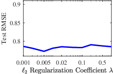
Among them, is a parameter for all TSK fuzzy systems, not specific to MBGD-RDA; can be determined by early-stopping on a validation dataset; and, , , , and are AdaBound parameters, whose default values are usually used. So, we only studied the sensitivity of MBGD-RDA to , , and , which are unique to MBGD-RDA.
The results, in terms of the test RMSEs, on the PM10 dataset are shown in Fig. 4, where each experiment was repeated 100 times and the average test RMSEs are shown. In each subfigure, except for the hyper-parameter under consideration, the values for other parameters were: , , , , , , , , , and and are defined in (12) and (13), respectively. Clearly, MBGD-RDA is stable with respect to each of the four hyper-parameters in a wide range, which is desirable.


III-E Comparison with ANFIS
ANFIS [10] is an efficient algorithm for training TSK fuzzy systems on small datasets. This subsection compares the performance of MBGD-RDA with ANFIS on the first six smaller datasets.
The ANFIS structure of a two-input one-output TSK fuzzy system is shown in Fig. 5. It has five layers:
- •
Layer 1: The membership grade of on is computed, by (2).
- •
Layer 2: The firing level of each rule is computed, by (3).
- •
Layer 3: The normalized firing levels of the rules are computed, by (5).
- •
Layer 4: Each normalized firing level is multiplied by its corresponding rule consequent.
- •
Layer 5: The output is computed, by (6).
All parameters of the ANFIS, i.e., the shapes of the MFs and the rule consequents, can be trained by GD [10]. Or, to speed up the training, the antecedent parameters can be tuned by GD, and the consequent parameters by LSE [10].

In the experiment, we used the anfis function in Matlab 2018b, which does not allow us to specify a batch size, but to use all available training examples in each iteration. For fair comparison, in MBGD-RDA we also set the batch size to the number of training examples. anfis in Matlab has two optimization options: 1) batch GD for both antecedent and consequent parameters (denoted as ANFIS-GD in the sequel); and, 2) batch GD for antecedent parameters, and LSE for consequent parameters (denoted as ANFIS-GD-LSE in the sequel). We compared MBGD-RDA with both options.
The training and test RMSEs, averaged over 10 runs, are shown in Fig. 6. MBGD-RDA always converged much faster than ANFIS-GD, and its best test RMSE was also always smaller. Additionally, it should be emphasized that MBGD-RDA can be used also for big data, whereas ANFIS-GD cannot.


Interestingly, although ANFIS-GD-LSE always achieved the smallest training RMSE, its test RMSE was almost always the largest, and had large oscillations. This suggests that ANFIS-GD-LSE had significant overfitting. If we could reduce this overfitting, e.g., through regularization, then ANFIS-GD-LSE could be a very effective TSK fuzzy system training algorithm for small datasets. This is one of our future research directions.
Fig. 6 shows the learning rates of ANFIS-GD, ANFIS-GD-LSE and MBGD-RDA. For the first two ANFIS based approaches, all model parameters shared the same learning rate. However, in MBGD-RDA, different model parameters had different learning rates, and we show the average learning rate across all model parameters on each dataset. The learning rates in ANFIS-GD and ANFIS-GD-LSE first gradually increased and then decreased. Interestingly, the learning rate of ANFIS-GD-LSE was almost always smaller than that of ANFIS-GD when the number of iterations was large. The learning rate of MBGD-RDA was always very high at the beginning, and then rapidly decreased. The initial high learning rate helped MBGD-RDA achieve rapid convergence.
III-F Comparison with DropMF and DropMembership
In addition to DropRule, there could be other DropOut approaches in training a TSK fuzzy system, e.g.,
- 1.
DropMF, in which each input MF is dropped with a probability , as illustrated in Fig. 7. Dropping an MF is equivalent to setting the firing level of that MF to 1 (instead of 0). Comparing DropMF in Fig. 7 and DropRule in Fig. 1, we can observe that each DropRule operation reduces the number of used rules by one; on the contrary, DropMF does not reduce the number of used rules; instead, it reduces the number of antecedents in multiple rules by one.


Fig. 7: DropMF, where is the th MF in the th input domain. (a) The red cross indicates that MF for will be dropped; (b) the equivalent fuzzy system after dropping . - 2.
DropMembership, in which the membership of an input in each MF is dropped with a probability , as illustrated in Fig. 8. Dropping a membership is equivalent to setting that membership to 1 (instead of 0). Comparing DropMembership in Fig. 8 and DropMF in Fig. 7, we can observe that DropMembership has a smaller impact on the firing levels of the rules than DropMF. For example, in Fig. 7, both and are impacted by DropMF, whereas in Fig. 8, only is impacted by DropMembership.


Fig. 8: DropMembership, where is the th MF in the th input domain. (a) The red cross indicates that membership in the first rule will be dropped; (b) the equivalent fuzzy system after dropping in the first rule.
Next, we compare the performances of DropMF, DropMembership with DropRule, by replacing DropRule in MBGD-RDA by DropMF and DropMembership, respectively. The training and test RMSEs, averaged over 10 runs, are shown in Fig. 9. Generally, DropRule performed the best, and DropMembership the worst. Comparing Figs. 1, 7 and 8, we can observe that DropRule introduces the maximum change to the TSK fuzzy system structure, and DropMembership the smallest. This suggests that a dropout operation that introduces more changes to the TSK fuzzy system may be more beneficial to the training and test performances.

III-G Comparison with Adam
We also compared the performances of AdaBound with Adam. The learning algorithm, MBGD-RD-Adam, was identical to MBGD-RDA, except that AdaBound was replaced by Adam, by setting and in Algorithm 1.

The training and test RMSEs, averaged over 10 runs, are shown in Fig. 10. MBGD-RDA converged faster than, or equally fast with, MBGD-RD-Adam, and had smaller or comparable best test RMSEs as MBGD-RD-Adam on most datasets. So, it is generally safe to choose AdaBound over Adam.
IV Conclusion and Future Research
TSK fuzzy systems are very useful machine learning models for regression problems. However, to our knowledge, there has not existed an efficient and effective training algorithm that enables them to deal with big data. Inspired by the connections between TSK fuzzy systems and neural networks, this paper extended three powerful optimization techniques for neural networks, e.g., MBGD, regularization, and AdaBound, to TSK fuzzy systems, and also proposed three novel techniques (DropRule, DropMF, and DropMembership) specifically for training TSK fuzzy systems. Our final algorithm, MBGD-RDA, which integrates MBGD, regularization, AdaBound and DropRule, can achieve fast convergence in training TSK fuzzy systems, and also superior generalization performance in testing. It can be used for training TSK fuzzy systems on datasets of any size; however, it is particularly useful for big datasets, for which currently no other efficient training algorithms exist. We expect that our algorithm will help promote the applications of TSK fuzzy systems, particularly to big data.
Finally, we need to point out that we have not considered various uncertainties in the data, e.g., missing values, wrong values, noise, outliers, etc., which frequently happen in real-world applications. Some techniques, e.g., rough sets [36], could be integrated with fuzzy sets to deal with them. Or, the type-1 TSK fuzzy systems used in this paper could also be extended to interval or general type-2 fuzzy systems [1, 37] to cope with more uncertainties. These are some of our future research directions.
References
- [1] J. M. Mendel, Uncertain rule-based fuzzy systems: introduction and new directions, 2nd ed. Springer, 2017.
- [2] A. Nguyen, T. Taniguchi, L. Eciolaza, V. Campos, R. Palhares, and M. Sugeno, “Fuzzy control systems: Past, present and future,” IEEE Computational Intelligence Magazine, vol. 14, no. 1, pp. 56–68, 2019.
- [3] I. Couso, C. Borgelt, E. Hullermeier, and R. Kruse, “Fuzzy sets in data analysis: From statistical foundations to machine learning,” IEEE Computational Intelligence Magazine, vol. 14, no. 1, pp. 31–44, 2019.
- [4] X. Gu, P. Angelov, and H.-J. Rong, “Local optimality of self-organising neuro-fuzzy inference systems,” Information Sciences, vol. 503, pp. 351–380, 2019.
- [5] X. Gu and P. Angelov, “Self-boosting first-order autonomous learning neuro-fuzzy systems,” Applied Soft Computing, vol. 77, pp. 118–134, 2019.
- [6] D. Wu and W. W. Tan, “Genetic learning and performance evaluation of type-2 fuzzy logic controllers,” Engineering Applications of Artificial Intelligence, vol. 19, no. 8, pp. 829–841, 2006.
- [7] L.-X. Wang and J. M. Mendel, “Back-propagation of fuzzy systems as nonlinear dynamic system identifiers,” in Proc. IEEE Int’l Conf. on Fuzzy Systems, San Diego, CA, 1992, pp. 1409–1418.
- [8] D. E. Rumelhart, G. E. Hinton, and R. J. Williams, “Learning representations by back-propagating errors.” Nature, vol. 323, pp. 533–536, 1986.
- [9] C.-T. Lin and C. S. G. Lee, Neural Fuzzy Systems: a Neuro-Fuzzy Synergism to Intelligent Systems. Upper Saddle River, NJ: Prentice Hall, 1996.
- [10] J. R. Jang, “ANFIS: adaptive-network-based fuzzy inference system,” IEEE Trans. on Systems, Man, and Cybernetics, vol. 23, no. 3, pp. 665–685, 1993.
- [11] M. Chen, S. Mao, and Y. Liu, “Big data: A survey,” Mobile Networks and Applications, vol. 19, no. 2, pp. 171–209, 2014.
- [12] X. Wu, X. Zhu, G.-Q. Wu, and W. Ding, “Data mining with big data,” IEEE Trans. on Knowledge and Data Engineering, vol. 26, no. 1, pp. 97–107, 2014.
- [13] A. McAfee, E. Brynjolfsson, T. H. Davenport, D. Patil, and D. Barton, “Big data: the management revolution,” Harvard Business Review, vol. 90, no. 10, pp. 60–68, 2012.
- [14] I. Jolliffe, Principal Component Analysis. Wiley Online Library, 2002.
- [15] I. Goodfellow, Y. Bengio, and A. Courville, Deep Learning. Boston, MA: MIT Press, 2016, http://www.deeplearningbook.org.
- [16] Y. Bengio, “Practical recommendations for gradient-based training of deep architectures,” in Neural Networks: Tricks of the Trade, 2012, pp. 437–478.
- [17] S. Nakasima-López, J. R. Castro, M. A. Sanchez, O. Mendoza, and A. Rodríguez-Díaz, “An approach on the implementation of full batch, online and mini-batch learning on a Mamdani based neuro-fuzzy system with center-of-sets defuzzification: Analysis and evaluation about its functionality, performance, and behavior,” PLOS ONE, vol. 14, no. 9, pp. 1–40, 2019.
- [18] B. T. Polyak and A. B. Juditsky, “Acceleration of stochastic approximation by averaging,” SIAM Journal on Control and Optimization, vol. 30, no. 4, pp. 838–855, 1992.
- [19] J. Duchi, E. Hazan, and Y. Singer, “Adaptive subgradient methods for online learning and stochastic optimization,” Journal of Machine Learning Research, vol. 12, pp. 2121–2159, 2011.
- [20] T. Tieleman and G. Hinton, “Lecture 6.5–RMSProp: Divide the gradient by a running average of its recent magnitude,” COURSERA: Neural Networks for Machine Learning, vol. 4, no. 2, pp. 26–31, 2012.
- [21] D. P. Kingma and J. Ba, “Adam: A method for stochastic optimization,” in Proc. 3rd Int’l Conf. on Learning Representations, San Diego, CA, May 2015.
- [22] S. Matsumura and T. Nakashima, “Incremental learning for SIRMs fuzzy systems by Adam method,” in Joint 17th World Congress of Int‘l Fuzzy Systems Association and 9th Int’l Conf. on Soft Computing and Intelligent Systems, Otsu, Japan, June 2017, pp. 1–4.
- [23] N. Yubazaki, J. Yi, M. Otani, and K. Hirota, “SIRMs dynamically connected fuzzy inference model and its applications,” in Proc. 7th IFSA World Congress, Prague, Czech Republic, Jun. 1997, pp. 410–415.
- [24] L. Luo, Y. Xiong, Y. Liu, and X. Sun, “Adaptive gradient methods with dynamic bound of learning rate,” arXiv preprint arXiv:1902.09843, 2019.
- [25] T. A. Johansen, “Robust identification of Takagi-Sugeno-Kang fuzzy models using regularization,” in Proc. 5th IEEE Int’l Conf. on Fuzzy Systems, New Orleans, LA, Sep. 1996, pp. 180–193.
- [26] Y. Jin, “Fuzzy modeling of high-dimensional systems: complexity reduction and interpretability improvement,” IEEE Trans. on Fuzzy Systems, vol. 8, no. 2, pp. 212–221, 2000.
- [27] E. Lughofer and S. Kindermann, “SparseFIS: Data-driven learning of fuzzy systems with sparsity constraints,” IEEE Trans. on Fuzzy Systems, vol. 18, no. 2, pp. 396–411, 2010.
- [28] M. Luo, F. Sun, and H. Liu, “Dynamic T-S fuzzy systems identification based on sparse regularization,” Asian Journal of Control, vol. 17, no. 1, pp. 274–283, 2015.
- [29] E. Lughofer and S. Kindermann, “Improving the robustness of data-driven fuzzy systems with regularization,” in Proc. IEEE Int’l Conf. on Fuzzy Systems, Hong Kong, China, Jul. 2008, pp. 703–709.
- [30] N. Srivastava, G. Hinton, A. Krizhevsky, I. Sutskever, and R. Salakhutdinov, “Dropout: A simple way to prevent neural networks from overfitting,” Journal of Machine Learning Research, vol. 15, no. 1, pp. 1929–1958, 2014.
- [31] L. Wan, M. Zeiler, S. Zhang, Y. LeCun, and R. Fergus, “Regularization of neural networks using DropConnect,” in Proc. Int’l Conf. on Machine Learning, Atlanta, GA, June 2013, pp. 1058–1066.
- [32] D. Wu, C.-T. Lin, J. Huang, and Z. Zeng, “On the functional equivalence of TSK fuzzy systems to neural networks, mixture of experts, CART, and stacking ensemble regression,” IEEE Trans. on Fuzzy Systems, 2019, accepted.
- [33] D. Wu, “Twelve considerations in choosing between Gaussian and trapezoidal membership functions in interval type-2 fuzzy logic controllers,” in Proc. IEEE World Congress on Computational Intelligence, Brisbane, Australia, June 2012.
- [34] A. J. Smola and B. Schölkopf, “A tutorial on support vector regression,” Statistics and Computing, vol. 14, no. 3, pp. 199–222, 2004.
- [35] A. E. Hoerl and R. W. Kennard, “Ridge regression: Biased estimation for nonorthogonal problems,” Technometrics, vol. 12, no. 1, pp. 55–67, 1970.
- [36] Z. Pawlak, Rough sets: Theoretical aspects of reasoning about data. Springer Science & Business Media, 2012, vol. 9.
- [37] D. Wu, “On the fundamental differences between interval type-2 and type-1 fuzzy logic controllers,” IEEE Trans. on Fuzzy Systems, vol. 20, no. 5, pp. 832–848, 2012.