Reconstruction of R-regular Objects from Trinary Images
Abstract.
We study digital images of -regular objects where a pixel is black if it is completely inside the object, white if it is completely inside the complement of the object, and grey otherwise. We call such images trinary. We discuss possible configurations of pixels in trinary images of -regular objects at certain resolutions and propose a method for reconstructing objects from such images. We show that the reconstructed object is close to the original object in Hausdorff norm, and that there is a homeomorphism of taking the reconstructed set to the original.
1. Introduction
The purpose of this paper will be to introduce a way to reconstruct objects from their grey-scale digital images. More specifically, we focus on objects that are small compared to the image resolution and satisfy a certain regularity constraint called -regularity. The notion of -regularity was developed independently by Serra [6] and Pavlidis [5] to describe a class of objects for which reconstruction from digital images preserved certain topological features. They both consider subset digitisation, that is, digitisation formed by placing an image grid on top of an object and then colouring an image cell black if its midpoint is on top of the object, and white if the cell midpoint is on top of the complement of the object. This way a binary image is produced, and they consider the set of black cells as the reconstructed set. Serra showed that if the grid is hexagonal and the object satisfies certain constraints, the original and reconstructed sets have the same homotopy, and Pavlidis showed that for a square grid and for certain -regular sets, the set and its reconstruction are homeomorphic. Later on, Stelldinger and Köthe [8],[9] argued that the concepts of homotopies or homeomorphisms were not strong enough to fully capture human perception of shape similarity. Instead they proposed two new similarity criterions called weak and strong -similarity, and showed that under certain conditions, an -regular set and its reconstruction by a square grid are both weakly and strongly -similar. We, too, will consider the notion of weak -similarity in this paper.
However, Serra, Pavlidis, Stelldinger and Köthe were modelling images using subset digitisation, which outputs a binary image. In contrast to this approach, Latecki et al. [4] modelled an image by requiring that the intensity in each pixel be a monotonic function of the fraction of that object covered by that pixel. This way they seek to model a pixel intensity as the light intensity measured by a sensor in the middle of the pixel, and the result is a grey-level image much like the ones obtained in real situations. They show that after applying any threshold to such an image of an -regular object with certain constraints, the set of black pixels has the same homotopy type as the original object and, in the case where the original object is a manifold with boundary, the two are even homeomorphic. They also conjecture that all -regular objects are manifolds with boundary. This was later proven by Duarte and Torres in [2].
We will model our images in the same way as Latecki et al. did, namely by requiring each pixel intensity to be a monotonic function of the fraction of the pixel covered by the object. In contrast to the above reconstruction approaches, we do not wish to use a set of pixels as our reconstructed set, but rather to construct a new set with smooth boundary that we may then use as the reconstruction. Also in contrast to the above, we will not consider binary images, but keep the information stored in the grey values in our endeavour to make a more precise reconstruction.
When reconstruction, one should decide which properties one wishes the reconstructed object to share with the original one. Should the reconstructed set have the same topological features as the original one? Should the reconstructed set be close to the original one? Should a digitisation of the reconstructed set yield the same image as the original set? Should the reconstructed set be -regular for some close to ? Though all of these comparison criteria are interesting to work with and an ideal reconstruction should satisfy them all, it is hard to construct such a set. In this paper, we will therefore focus on constructing a set that is close to the original one in Hausdorff distance (which will be introduced in the following), has a smooth boundary, and is homeomorphic to the original set. This means that we show that our reconstructed set and the original are weakly -similar in the sense of [9].
2. Basic definitions and theorems about -regular sets
Let us start by establishing some terminology. Let be a set. We will denote the closure of by , the interior of by and the boundary of by . The complement will be denoted by . The set is compact if and only if is closed and bounded.
The Euclidean distance between two points and in will be denoted by or, occasionally, by .
For an , we let be the open ball with centre and radius . For a line segment we will denote the length of by .
A part of the goal will be to construct a set from a digital image whose boundary is close to the boundary of the original set. The intuitive concept of closeness between two sets is captured by the Hausdorff distance: For , the Hausdorff distance between and is given by
The set of compact sets of equipped with the Hausdorff metric is a complete metric space.
The digital images that we will be working with in this paper are formed in the following way:
Definition 2.1.
Let be a set and a grid with side length . To each grid square , we assign an intensity given by
where is a monotonic function with , and .
The digitisation of is the matrix of intensities. We will visualise it as the collection of pixels of side length , each coloured a shade of grey corresponding to the value of .
Let denote the black pixels of this digitisation of . We will sometimes refer to as the black digitisation pixels of .
To make sure that the objects in the images we are considering are not arbitrarily strange, we will follow in the footsteps of previous approaches and only consider -regular sets:
Definition 2.2.
Let . A closed set is said to be -regular if for each there exists two -balls and such that , see Fig. 1.

In general, we believe that a reconstruction can be made more accurately by taking the intensities of the grey pixels into account, and we are currently working on this idea. However, in this paper we restrict ourselves to looking at images where each pixel is considered to be either black, grey or white, without taking the exact intensities of the grey pixels into account:
Definition 2.3.
A trinary digital image is a digital image where the intensities of all grey pixels are set to 0.5.
These trinary images will be our main interest in this paper. Note that the colour of a pixel (black, grey or white) does not depend on the monotonic function used for calculating the pixel intensities - in fact, a pixel in a trinary image of an object is black if it is contained in , white if it is contained in and grey if passes through it.
When we make the digital image of an -regular object by a lattice , we can in general not be certain that there are any black or white pixels in the image - for instance, if is large compared to , all pixels could contain an -ball, which would mean that the image would be all grey. Since we cannot hope to make a very good reconstruction in this case, we will put a restriction on the relationship between the and :
Convention.
Throughout the following, we assume that is a bounded -regular set and that . We also assume that does not pass through a pixel corner.
Note that the boundedness condition on implies that is compact.
Pavlidis [5] defines a grid and a set to be compatible if is -regular with . With this restriction, since is the diameter of a pixel, each black -ball contains the pixel that its centre belongs to, meaning that each black -ball is centered in a black pixel. Similarly the centre of each white -ball is contained in a white pixel. This means that for each component of yields at least one black pixel, and each component of yields at least one white pixel. Latecki et al. showed that for a compatible grid and set , the set of black pixels is homeomorphic to . Hence and have the same topological features. Furthermore, the above conditions ensure that we do not get too large grey areas, as will be clear in the following section. We will only concern ourselves with images that capture all of the objects photographed, and not just a part of them.
Definition 2.4.
Let be bounded sets and . We call and weakly -similar if there exists a homeomorphism such that and the Hausdorff distance between the set boundaries satisfies
The overall purpose of this paper will be to show the following:
Theorem 2.5.
Let be a digital image of an -regular set by a lattice with . We may construct an object from such that and are weakly -similar, where is the pixel side length.
We believe that the above result may be strengthened to prove strong -similarity between the two for a suitable , but such a result is beyond the scope of this paper.
A large part of the proof of Theorem 2.5 will be to prove the following:
Theorem 2.6.
Let be a digital image of an -regular set by a lattice with . We may construct an object from such that , where is the Hausdorff distance.
To start working with -regular sets, we first sum up some basic statements about them:
Proposition 2.7 (Tang Christensen and du Plessis, [1], Proposition A.1).
Let be a closed set and . Then the following are equivalent:
- (1)
At any point there exist two closed -balls and such that .
- (2)
The sets and are equal to unions of closed -balls.
Definition 2.8.
For , we denote the -tubular neighbourhood of in by .
Lemma 2.9 (Duarte & Torres, [2], Lemma 5).
Let be an -regular set. For each there is a unique point such that . Hence there is a well-defined projection .
Theorem 2.10 (Duarte and Torres, [3]).
The projection map is continuous.
Another important fact that we will be using heavily is the following:
There is a retraction (that we will sometimes just denote by ) defined by
and likewise a retraction defined by
These retractions will prove to be crucial in later arguments, since they have some nice properties.
We now state some results about . However, the similar results for also hold.
Proposition 2.11 (Stelldinger et al., [7]).
Let with and let be the line segment between them. Then
- (1)
The line segment is a subset of , and is injective,
- (2)
For and any -ball containing and , is a subset of .
Definition 2.12.
Let be a closed line segment of length . Then the -spindle around is the intersection of all closed balls of radius whose boundaries contain both endpoints of . If and are the endpoints of , we will sometimes write in stead of .
Lemma 2.13 (du Plessis, A.20 [1]).
Let be a closed line segment in of length . Then the maximal distance from a point in the -spindle to is .
Lemma 2.14 (du Plessis, A.13 [1]).
Let be a closed line segment of length . Then the -spindle is the intersection of all balls of radius at most that contain .
Corollary 2.15 (du Plessis, A.16 [1]).
Let with and let be the line segment between them. Then is a subset of the -spindle .
Remark 2.16.
Since , the above corollary is also true for .
3. Impossible configurations at a resolution satisfying
Before we start reconstructing the original -regular object, we need to discuss which configurations of pixels of grey, black and white pixels can occur in the digital image of an -regular object by a lattice where . We can make a computer put together all possible configurations of pixels by telling it that the only possible configurations of pixels are the ones in Figure 2, up to rotation and interchanging of black and white. We can then make a MatLab programme that combines these configurations in all possible ways. If we do this, we get (up to rotation, mirroring and switching of black and white pixels) the configurations in Figure 3.


Note that not all these configurations can occur in the image of some -regular object by a lattice with . We would like to remove configurations that do not occur from the list in Figure 3. To do so, we need to prove a series of lemmas. Their proofs are mainly geometric and rather technical, so we will put them in the appendix instead of presenting them here.
First of all, let us start with a definition, borrowed from Pavlidis’ book [5].
Definition 3.1.
Two pixels are direct neighbours (abbreviated d-neighbours) if the respective cells share a side. Two pixels are indirect neighbours (abbreviated i-neighbours) if those cells touch only at a corner. The term neighbour denotes either type.
In the following lemmas, we will only be considering pixel configurations in images of -regular objects by lattices with according to our convention, but for brevity we will omit this requirement from the lemma statements.
Lemma 3.2.
Consider four pixels as in Figure 4. Suppose intersects the edge between the two pixels and more than once. Then one of the pixels and is black, and the other one is white. The same result is true if is tangent to in a point.

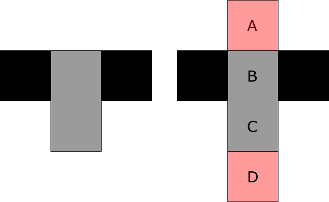
Lemma 3.3.
Lemma 3.4.
Consider a configuration of pixels with the middle one grey. Then one of its 8 neighbour pixels is not grey.

Lemma 3.5.
Consider a configuration of pixels as in Figure 6, where the middle one is grey and has centre . Let be the point of that is nearest to , and suppose the centre of the black ball tangent to at is closer than the centre of the white ball tangent to at , and that belongs to the lower left pixel (which is hence black).
Then the upper right pixel is white.

Remark 3.6.
Theorem 3.5 and Lemma 3.4 combined tell us that a grey pixel with four grey d-neighbours must always have a black and a white i-neighbour whose common vertices with sit diagonally across from each other, see Figure 7, left. Equivalently, if a grey pixel does not have a black and a white neighbour sitting opposite of each other, then at least one of its d-neighbours must not be grey.


Lemma 3.7.
The following holds:
- (1)
Consider pixels as in the lower part of Figure 8 with the grey and black pixels placed relatively to each other as in the figure. Then pixels and must necessarily be black.
- (2)
Consider pixels as in Figure 8, with the grey and black pixels placed relatively to each other as in the figure. Then must necessarily be black.
- (3)
Consider pixels as in Figure 8, with the grey and black pixels placed relatively to each other as in the figure. Then either the pixels , , are all black, or the pixels , , are all black.
The similar result is also true if we replace the black pixels with white ones in the figures.

Lemma 3.8.
Suppose we have a configuration of 6 grey pixels as in Figure 9, with pixels , , and as in the figure. Then the following holds:
- (1)
One of the pixels , must be black, and the other one white,
- (2)
The set belongs to the set of points in that are no further than from the common edge of (i.e. the red set in the figure).
Lemma 3.9.
A configuration as the one in Figure 10 left cannot occur.


Lemma 3.10.
A configuration as the one in Figure 11, left cannot occur.
Theorem 3.11.
Up to rotation, mirroring and interchanging of black and white, any configuraton of pixels is one of those shown in Figure 12.

In the following, it will also be useful to know which -configurations with a centre of grey pixels that may occur in a digital image of an -regular object by a lattice . We may have a computer find these by combining all possible -configurations from Figure 12, together with the rotations, mirror images and inverses of these configurations. After removing configurations that violate Lemma 3.8, this yields the configurations in Figure 13 (up to rotations, mirror images and interchanging of black and white). We aim to remove configurations from this list if they cannot occur in a digital image like the ones we are considering.

Lemma 3.12.
The configuration in Figure 14 cannot occur.


Lemma 3.13.
The left configuration in Figure 15 cannot occur.
Lemma 3.14.
The boundary cannot intersect all four boundary edges of a configuration of grey pixels.
Theorem 3.15.
The only possible configurations of -configurations with grey pixels in the middle are the ones shown in Figure 16.

Note that the converse is not true: There are configurations in Figure 16 that does not occur in any image of an -regular object by a lattice with . But since the proofs of this is rather technical and the result is not relevant to our further progress, we will not discuss them here.
4. Reconstruction of the boundary of the set
All the work done in the previous section was leading up to the development of a reconstruction algorithm, which we will introduce in this section. The idea will be to use circle arcs to approximate the boundary of the edge. The reconstructed set will not in general be -regular.
Before we start, we will introduce some points, called auxiliary points, that our reconstructed boundary must pass through. These are defined differently for different grey pixels. Hence we define
Definition 4.1.
A grey pixel sitting in a configuration of grey pixels is called complex. A grey pixel that is not sitting in a configuration of grey pixels is called simple.
We now introduce the auxiliary points needed for the reconstruction.
Consider a pixel edge shared by two grey pixels and . If the two grey pixels sit in the same configuration of grey pixels, we introduce an auxiliary point at the midpoint of this configuration. If they do not, we introduce a point on the midpoint of their common edge, see Figure 17. (Note that the two grey pixels may be part of two different configurations of grey pixels. In that case, we introduce two auxiliary points, on at the centre of each of the two configurations).

Lemma 4.2.
All simple grey pixels have between one and three auxiliary points on their boundary. All complex grey pixels have either one or two grey auxiliary points on their boundary.
Proof.
Lemma 4.3.
A simple pixel with just one auxiliary point on its boundary must share this point with a simple pixel with three auxiliary points on its boundary. On the other hand, a simple pixel with three auxiliary points on its boundary must share exactly one of these points with a simple pixel with just one auxiliary point on its boundary.
Proof.
Check all cases as presented in Figure 12. ∎
We will now remove the auxiliary point of all simple pixels that has only one auxiliary point. By the above lemmas, this now means that all simple pixels have zero or two auxiliary points on their boundary, and all complex pixels have one or two auxiliary points on their boundary.
Lemma 4.4.
In each configuration of grey pixels there are exactly 3 auxiliary points - one at the centre and two on the configuration boundary.
Proof.
Each -configuration of grey pixels sits in one of the configurations in Figure 16 (up to rotation, mirroring and switching of colours). Hence we get the above theorem by checking all possible cases. ∎
Theorem 4.5.
For each auxiliary point , there are exactly two auxiliary points with the property that there is a pixel having both and that auxiliary point on its boundary.
Proof.
Consider an auxiliary point , sitting on the boundary of pixel . If is the centre of some configuration of black pixels, then by Lemma 4.4 there are only two auxiliary points on the boundary of this configuration as claimed.
If is the midpoint of some pixel edge, consider a pixel having this edge. It is either simple (and hence has two auxiliary points on its boundary), or it is complex and hence has an auxiliary point in a corner of . In both cases, there is exactly one other auxiliary point on the boundary of each of the pixels having on their boundaries. ∎
The above theorem means that there is a natural way of defining ’neighbouring auxiliary points’: Two auxiliary points are neighbours if they sit on the boundary of the same pixel.
The next step is to approximate the boundary of with curve segments: Consider an auxiliary point and its two neighbour auxiliary points. We approximate by circle arc segments through these three points (or, if the points are collinear, by line segments). Hence there are two curve segments through each two neighbouring auxiliary points sitting on the boundary of the same pixel , one starting in one of the points, the other ending in the other point. Each of these curve segments are graphs over the straight line through the points, so we may write them as and . Then choosing a bump function with and , we may patch a connected curve together by putting in each pixel , see Figure 18. The resulting curve is then also a graph over , and the curve is a smooth embedded submanifold of .

Lemma 4.6.
The path is contained in the area bounded by and .
Proof.
Since is a graph over a line and it is a convex combination of a point on and a point on , the curve must lie between these two points, and hence also between the curves and . ∎

Lemma 4.7.
Consider two neighbour auxiliary points on the boundary of some pixel not sitting in a configuration like the ones in 19.
- •
If the two neighbour auxiliary points do not sit at the endpoints of some edge of , then the curve is contained in .
- •
If the two neighbour auxiliary points do sit at the endpoints of the edge shared by and some other pixel , then the curve is contained in .

Proof.
We start by proving the lemma for the arc segments and : We can consider all possible positions of three neighbour auxiliary points, see Figure 20. Look at auxiliary points , sitting in configurations around a red pixel like any of the five figures to the left. A calculation (or a look at the figures!) then show that with the exception of auxiliary points in configurations as the ones shown in Figure 19, all possible circle arcs through two auxiliary points sitting on a red pixel are contained in that red pixel.
Proposition 4.8.
The curves have no self-intersections, and do not intersect each other. Hence each component of is a simple closed curve.
Proof.
Since each segment is a graph over some straight line , we only need to show that two segments and do not intersect. By Lemma 4.6 it suffices to show that the area bounded by two arcs and in a pixel does not intersect the area bounded by two arcs and in another pixel .
Consider the possible circle arcs shown in Figure 20. With the exception auxiliary points sitting in configurations like the ones in Figure 19, all arc segments stays inside the pixel(s) containing both of the auxiliary points they join. Since no pixel can have more than two auxiliary points on their boundary, the only possible way that two curve segments can intersect is if one of them, say , is made using a curve connecting points in a configuration like the one in Figure 19. But going through all possible configurations where such a could occur one can conclude that cannot intersect itself in this case either.
That each segment of is a simple closed curve follows from the fact that the segments always connect two neighbour auxiliary points, and all auxiliary points have two neighbours. If a component of were not a closed curve, it would have an endpoint (since all components of are bounded) - but is the join of curve segments between neighbour auxiliary points, so such an endpoint can only occur in one of the auxiliary points. But since all auxiliary points have two neighbour auxiliary points, this is impossible. ∎
Theorem 4.9.
For each component of , there is exactly one component of . Each component of separates the boundary components of a connected component of the set of grey pixels.
Proof.
Let be a component of , and let be the set of grey pixels containing points of . Note that cannot have any grey neighbour pixel , because this would imply that contained a point from another component of , which would mean that there were two points on different components of closer than - a contradiction by Corollary 2.15 applied to . Hence is a connected component of the set of grey pixels.
Consider any chain of grey pixels in , where each pixel in the chain is a neighbour of the previous and the next pixel in the chain, and each pixel appear in the chain no more than once. Assume that the start pixel and end pixel of the chain has at least two grey d-neighbours. We aim to show that the first and last pixel in such a chain is connected by a segment of .
By construction, each pixel in such a chain has at least two grey d-neighbours, hence has at least one auxiliary point on its boundary. If a pixel in the chain has only one auxiliary point on its boundary, its two grey d-neighbours must sit in a configuration with , and hence one of its grey d-neighbours must have two auxiliary points on its boundary. Hence if we replace by its d-neighbours with two auxiliary points on their boundary, we still get a chain of pixels in . Repeating this, we end up with a chain of pixels where all pixels in the chain have two auxiliary points on their boundary. The construction of then yields a segment of through this pixel chain.
Now by -regularity of , must be larger than 2 pixels and hence have at least one pixel with two grey d-neighbours. Hence contains at least one component of . If contained two components , of , we could pick a chain of grey pixels connecting a pixel containing a point of with a pixel containing a point of . Then by the above, the auxiliary points on the first pixel would be connected to the auxiliary points on the last pixel by a segment of . But then and would be connected - a contradiction. Thus for any component of , there is exactly one component of .
For the second part of the statement, consider a chain of pixels following a boundary component of . By the above, this chain yields a segment of which is a closed curve containing , but not containing any other components of the boundary of . Hence separates any component of from the others - in particular, there can be at most two boundary components of , and separates them. In fact, there are always two components of : Any point has a black and a white -ball osculating at , and these balls contain the pixels in which they are centred. Since separates the two balls and hence the two pixels where they are centred, so does . But then must have two different boundary components, and both and separates these two components. ∎
Since the set of grey pixels separates the white pixels from the black, the above theorem actually implies that also separates the white pixels from the black (in the sense that any curve from a black to a white pixel must intersect ). We may conclude (via the Jordan Curve Theorem) that each component of separates into two sets, a bounded and an unbounded. From now on, is the boundary of the reconstructed set, which we define as follows:
Definition 4.10.
We define the reconstructed set to be the bounded set having as boundary.
5. Hausdorff distance between the boundaries of the original set and the reconstruction
We are now ready to look at the Hausdorff distance between our reconstruction and the original object. Let us start by proving a lemma:

Lemma 5.1.
Consider a grey pixel as the one in Figure 21, with two black (or two white) neighbour pixels sharing a vertex. Let be the vertex of that does not belong to the two black (or white) neighbour pixels. If , then .
Proof.
Let be as above. Then belongs to a component of that must enter and leave in two places, say in points and . These points belong to one of the edges of having as a corner. Let be the line segment between and .
Now that we have a suggestion for the boundary of the original set, we aim to show how good this approximation is. The first step will be to prove the following:
Theorem 5.2.
Any point of has distance at most to the curve consisting of curve segments . Hence .
This theorem, however, requires some additional lemmas:
Lemma 5.3.
If two neighbour auxiliary points sit on the common boundary edge of two grey pixels and , then the curve is contained in the set of points in that are at a distance from the common edge of .
Proof.
If two auxiliary points sit at the common boundary edge of and , they must sit on the ends of , i.e. they are the two common vertices of and .
By Lemma 4.7, part ii), belongs to . Let and be the two arc segments whose merge is . Then they are both circle arcs of radius no smaller than (see Figure 20), hence they are contained in the spindle whose height is . Thus no point of or is further away than from . Since the curve belongs to he area bounded by and by Lemma 4.6, we must also have that belongs to . ∎
Lemma 5.4.
If two auxiliary points sit on two edges of a pixel sharing a corner , then is contained in .
Proof.
We already know from Lemma 4.7 that belongs to . Hence we only need to show that belongs to . By Lemma 4.6 it suffices to show that the area between the two curves and belongs to and, since is convex, it is even enough to show that and both belong to . This can be done by a calculation for all possible cases, or by looking at Figure 22. ∎
Lemma 5.5.
If two neighbour auxiliary points on the boundary of some pixel do not sit on the same edge of and neither in a configuration as the ones in Figure 19, then the distance between any point of in and the curve is less than .
Proof.
Consider two auxiliary points on the boundary of pixel . Suppose they sit on two opposite edges , of . If furthermore the two points do not sit in one of the configurations of Figure 19, then by Lemma 4.7, the curve belongs to . Hence the curve must run from one side of to the other without leaving , see Figure 22 left. Thus given any point in , projecting it to along a line parallel to moves it no further than a distance . Hence all points of is closer than to .

On the other hand, suppose the two auxiliary points on the boundary of sit on the midpoint of two edges , sharing a vertex , see Figure 22 right. Then is a simple pixel, and since its auxiliary points do not sit on opposite edges, it cannot be one of the simple pixels that we removed auxiliary points from (by the proof of Lemma 4.3). So must have two grey d-neighbour pixels sharing the vertex , and two non-grey d-neighbour pixels sharing the vertex opposite of , as in Figure 22 right. Let us assume these two non-grey pixels to be black.
Consider at point . By Lemma 5.1, must belong to . Then since the path is also contained in this ball by Lemma 5.4 and runs from to , we hit somewhere if we move a point in along a radius of . Such a movement displaces the point a distance of at most , since this is the maximal distance between a point on and a point on on the same radius of . Hence a point of is at most a distance from . ∎
Proof of Theorem 5.2.
By Lemma 5.5 the theorem holds for any point of contained in a pixel with two auxiliary points not sitting on the same edge, and not sitting in one of the configurations of Figure 19. Hence we need to show the result for points on contained in i) grey pixels with two auxiliary points sitting on the same edge, ii) the special cases in Figure 19, iii) grey pixels with one auxiliary point on their boundary and iv) grey pixels with zero auxiliary points on their boundaries.
Ad i): By Lemma 5.3, must belong to the set of points in closer than to , and by Lemma 3.8, all points of in must be closer than to . Since the curve runs from one side of to the other, then pushing a point orthogonally to inside , we must hit at some point. The displacement made in this manner can be no larger than , hence any point of is closer than to .

Ad ii): Now consider instead either of the cases from Figure 19. Such a configuration must necessarily sit in a configuration like in Figure 23, by looking at the possible configurations involving grey pixels in Figure 16. We will aim to show that the rectangle in the figure, which shares two vertices with pixel and has the other two vertices at the midpoints of the vertical pixel edges of , does not contain any points of .
Look at the blue line separating the two upper grey pixels from the lower. Since there are grey pixels on both sides of , must pass it somewhere, and since both endpoints of are black, must pass at least twice. Then there must be some point in one of the two upper pixels where has horisontal tangent, and hence the centres of the black and white -balls meeting at this point sit on the vertical line through . Since the pixels above the grey are black in the figure, the upper ball osculating at must be black, and the lower must be white.
By Corollary 2.15 applied to the part of between two points in must be contained in the spindle (shown in the figure), which contains points no further from than . So cannot be further above than .
Now if belonged to the right upper grey pixel, the centre of the white ball osculating at would belong to a grey pixel and hence colour that pixel white. So this is not possible. Therefore must belong to the upper left pixel, and be no further from then . The centre of the white -ball osculating at must therefore lie in the white pixel, no further than from and hence no further from the common edge between the white pixel and than (so somewhere in the light blue part of this white pixel). But any -ball centred centred in the top half of the white pixel must contain , the bottom half of pixel , since and the top half of form a square with side length Hence the white ball osculating at must contain all of , so cannot contain any points of .
A calculation shows that no point of lies further above than . Hence if we take any point in and push it along a vertical line to , we can do this without moving more than a distance away. So any point of is closer than to .


Ad iii): Consider a grey pixel with only one auxiliary point on its boundary. By construction must be complex and have two grey neighbour pixels, and two non-grey neighbour pixels, see Figure 25. By Lemma 5.1 all points of must belong to the ball . Hence the distance from a point in to is less than . Since belongs to , this shows the claim in this case.
Ad iv): Consider a grey pixel without any auxiliary points on its boundary. By construction, it means that is a simple grey pixel with one grey d-neighbour pixel , and three non-grey d-neighbour pixels, see Figure 25.
Now, the boundary must pass the common edge of or in order to get into and out of . Hence the part of that is in must be contained in .But contains no points in that are further from than .
Furthermore, must have one auxiliary point on the midpoint of each vertical edge - let us call these and . Then an arc segment through and and a third auxiliary point of one of the grey pixels neighbouring must lie above the straight line connecting and (just look at all possible cases, as is done in Figure 25).
Hence any point in is closer than to , and any point in is closer than to . So the distance from to is less than . This finishes the proof that any point of is closer than to .
For any point in , there is a point in that is no further than a distance from , meaning that
Thus we get
∎
This proof is the first step on our way to show that and are close to each other in Hausdorff distance. The second step is taken when we prove the following
Theorem 5.6.
Any point of has distance at most to the boundary of the original set . Hence .
The proof of this theorem is very similar to the proof of Theorem 5.2. Again we split the proof in a couple of lemmas.
Lemma 5.7.
Consider a simple pixel with two auxiliary points on two opposite edges. Then any point of is closer than to some point of .


Proof.
Notice that must sit in one of the two configurations of Figure 27. In the first case, pick a point . The horisontal line in through has a black and a white endpoint, hence it must contain a point of . Since is no further than from the endpoints of this line, there must be a point in that is closer than to .
In the second case, pick again a point in . Let be the pixel above . Notice that must enter and leave by crossing in order for to be grey and both endpoints of to be black. Then by Corollary 2.15 with replaced by , any point of in must belong to the spindle which contains points no further from than by Lemma 2.13. So any point of must either belong to or be no further from than . On the other hand, a calculation shows that the path is closer than to .
Look at a vertical line in through . There must be a point on this line belonging to , since its endpoints have different colours. Either this point belongs to (in which case they can be no further apart than by the first part of the proof), or it belongs to . If it belongs to , it is no further from than , and since is no further than from , this point of must be closer than to . ∎
Lemma 5.8.
Consider a simple pixel with two auxiliary points, located at the midpoint of two vertex-adjacent edges of . Then no point of is further away from than .
Proof.
A pixel as the described must sit in a configuration as the one in Figure 27. Let denote the vertex of where the two edges containing auxiliary points meet. Let .
Consider then line in through and . Since it has endpoints of different colours, it must contain a point in . By Lemma 5.1, any point of must belong to the ball , and by Lemma 5.4, so must . Hence and both sit on a radius of the ball . By looking at the possible curves , such two points cannot be further apart than a distance . So any point is closer than to . ∎
Lemma 5.9.
Consider a complex pixel with two auxiliary points located at the endpoints of some edge of . Then no point of is further away from than .


Proof.
The pixel must sit in a configuration as the one in Figure 29, by means of Lemma 3.8. By Lemma 4.7, part ii) must belong to .
Now pick a point , and look at the vertical line in through . Since this line has endpoints of different colours, it must contain a point . By Lemma 3.8 again, must belong to the set of points in that are no further than from the common edge of and , and by Lemma 5.3 is no further than from . Hence and cannot be further than from each other. ∎
Lemma 5.10.
Consider a complex pixel with two auxiliary points located at vertices of diagonally opposite each other. Then no point of is further away from than .
Proof.
A pixel as in this lemma must sit in a configuration as the one in Figure 29, by means of Lemma 3.5. Let and denote the two auxiliary points on the boundary of .
A calculation shows that any circle arc through and an auxiliary point neighbouring has radius greater than . Hence any such circle arc is contained in the spindle where is the line segment between and , by Lemma 2.14. By the same lemma, this means that any such circle arc is contained in any ball of radius containing . The same holds for the area bounded by the two circle arcs and (since is also convex), and hence also for . Thus, if we can find some point in such that the -ball around contains and hence and , then any point of must be closer than to .
Consider the line connecting the black and white vertex of . Since its endpoints have different colours, it must contain some point . Since the distance between points of and , is less than everywhere, the ball contains and and hence the spindle between them, and we are done. ∎
Lemma 5.11.
Suppose is a complex pixel with an auxiliary point on one of its edge midpoints and another auxiliary point at one of the vertices of . Then any point of is closer than to .


Proof.
A pixel as the one in this lemma must sit in a configuration as the one shown in Figure 31.
There are two cases: Either is contained in or it is not.
Suppose first that . Note that must intersect the left vertical edge of once, since the endpoints of this edge has different colours. It cannot intersect the edge multiple times by Lemma 3.2. Let be the intersection between the left vertical edge of and .
Now, must intersect the boundary of in at least two points, one of which is . Suppose that intersects somewhere on the upper edge of , say in a point . Let be the line between and . Then by Corollary 2.15 there is a path in from to contained in , and by changing if necessary, we may assume that does not intersect the upper edge of except at , hence it stays inside . Let be the upper left vertex of .
Since contains the left and upper edge of , it contains both , and hence . Since , this also means that it contains by Lemma 2.14, hence it contains the path . It also contains , which can be seen by considering the possible cases in Figure 20.
Now, take any point on . Then it belongs to a radius of . Since runs from one side of to another inside , there must also be a point on lying on the same radius of as . But then and can be no further than apart, so the lemma is true in this case.
If on the other hand belongs to , but there are no points of on the upper edge of , then there must be a point on the right edge of . Let be the line between and . By Corollary 2.15, there must be a path in connecting and , and this path can nowhere intersect other edges of .
Again pick a point in , and look at the vertical line in containing . This line must be intersected by in some point , since connects the two sides of . But then and both lie on the same line of length , hence they can be no further than apart, as claimed. This concludes the proof in the case where is contained in .
Finally, assume is not contained in . Then one of the curve segments and are not contained in - let us say it is . Copying the results from before, we see that all points of inside are closer than to some point of , so it remains to show this for points of outside . Such points must lie in the set bounded by and one of the edges of (the red set in Figure 31).
Notice that the only case where the curve segment is not contained in is when sit in a configuration as the one in Figure 31. Let be the pixel above in this configuration.
The boundary must intersect the boundary of at least twice in order for to be grey. By Lemma 3.2, cannot intersect the right boundary of twice. Hence it must intersect the common edge of and at least once, say in a point .
Now, a calculation shows for any point , the ball contains all of . In particular, the ball contains all of and hence any point of in , so any such point can be no further away from than . This concludes the proof. ∎
Proof of Theorem 5.6.
The curve consists of a curve segments for each pixel with two auxiliary points on its boundary. Hence the theorem follows from the Lemmas 5.7, 5.8, 5.9, 5.10 and 5.11.
Furthermore, for any point in , there is a point in that is no further than a distance from , meaning that
Thus we get
∎
Corollary 5.12.
The reconstructed boundary is closer than to the boundary of .
6. Homeomorphism between Object and Reconstruction
Let us now finish the proof of Theorem 2.5. We need to show that there is homeomorphism taking the reconstructed set to the original set . To do so, let us start with a lemma:
Lemma 6.1.
Let be a set homeomorphic to , and let be the subset homeomorphic to . Let be a closed curve. Then there is a homeomorphism taking to fixing points in the unbounded component of .
Proof.
Since there exists a homeomorphism of taking the outer boundary component of to the unit circle by Schoenflies’ Theorem, we may assume that is the unit circle. By the Annulus Theorem, the set between and is homeomorphic to the annulus - let denote this homeomorphism. We may assume that is the identity on - if this is not the case, then after reversing the orientation of the map if necessary there is an isotopy from to which we may extend to an ambient isotopy of in a small tubular neighbourhood of in , and composing the result of this isotopy with we get a homeomorphism that is the identity on .
We may continuously extend to a map of all of by extending it by the identity on the unbounded component of (since the map may be extended to a map of the disc bounded by ) . Thus we get a map taking to and fixing points in the unbounded component of .
Repeating the above with replaced by , we also get a map taking to . Hence the composition takes to and fixes points in the unbounded component of . ∎
Theorem 6.2.
There is a homeomorphism taking to . Hence and are weakly -similar.
Proof.
Note that by Theorem 4.9 separates black pixels from white ones, and there is a 1-1 correspondence between components of and components of .
Consider an outermost component of . Since is a manifold of dimension , it is homeomorphic to . Thus its tubular neighbourhood is homeomorphic to (see [1], Proposition A.10) via a map that takes the points of each normal line of length to a fiber in , and takes to . Moreover, is a subset of the set of white pixels, and is a subset of the black pixels. Since the boundary of the reconstructed set separates black and white pixels, this means that there is a component of in .
Then by Lemma 6.1 there is a homeomorphism taking to and fixing points in the unbounded component of . Since and both separates black pixels from white, any component of inside also lies inside . Hence also takes any component of inside to the inside of .
Applying the above technique to the other components of , we thus get a series of homeomorphisms that each takes one component of to a component of . Since each homeomorphism fixes the points of the unbounded component of , the composition that starts by mapping the outer component(s) of to and then works its way in, sends to . Since it also sends bounded sets to bounded sets and was the bounded set bounded by and was compact, this means that takes to .
Since there is a map of taking to , and since by Corollary 5.12, they are weakly -similar. ∎
7. Example of the reconstruction algorithm
Example 7.1.
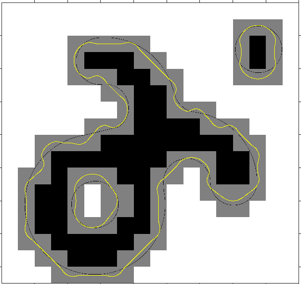
An example of this algorithm is shown in Figure 32. In this figure, we used the bump function
It seems from our example that the curves and may be even closer than .
8. Conclusion
In this paper we have presented restrictions on pixel configurations in digital images of -regular objects at a reasonable resolution. We have used these restrictions to reconstruct the original object by constructing an object with smooth boundary that is weakly -similar to the original object (where is the side length of each pixel). This tells us that our reconstruction is not far from the original object and has the right topology, and though that ensures that the sets are not fundamentally different, sadly it is not quite enough to cover all aspects of human perception of similarity, as discussed in [9], [7].Ongoing work is aiming at showing that the reconstructed object is in fact strongly -similar to the original one for a suitable .
We do by no means believe that a Hausdorff distance of between the original object and our reconstructed object is the optimal - in fact, we are working on obtaining even stronger bounds on their Hausdorff difference. We also believe that taking the actual intensities of each pixel into account can result in even more precise reconstruction, though there is still a lot of work to be done before we are ready to prove this.
The object that our reconstruction method outputs will in general not be -regular. We may, since the boundary of the reconstructed set consists of the join of finitely many curve segments, calculate the maximal curvature of a reconstructed set - but note that a maximal curvature or is not enough to ensure that our reconstructed set is -regular. Thus we have left the question of regularity of the reconstruction out of this paper, though it is also be an interesting aspect of the reconstruction process.
Appendix A Proofs of the lemmas from Section 3
We here include the proofs that were omitted in Section 3. To lighten the notation, we will measure distances in units of , so that each grid square has side length 1, and the assumption becomes .
Proof of Lemma 3.2.
Let and be two points on the common edge of and that belongs to , and let be the line segment between them. Note that since is -regular and , is in particular -regular (cf. [1], Proposition A.2).
Since the distance from to is less that , there must be a path in between them, where is the projection onto , see Section 2. Since the projection is continuous and fixed at the endpoints, there must be a point on such that the tangent to at is horisontal. Let . Since and is an -regular set, there are balls and such that , and since the tangent to at is horisontal, the centres and must lie on the vertical line through .
Note that . By Lemma 2.13, the thickness of is . So . Then
and
So belongs to either or - let us say . Then must be black. In fact, since the first and last inequality are sharp, the common edge of and must be interior points of , and hence it contains no intersection points. A symmetric argument for shows that must belong to , hence must be white, and that the common edge of and cannot contain any points of .
If is tangent to at a point , replacing with in the above argument shows the result. ∎
Proof of Lemma 3.3.
Let us name the two grey pixels in the configuration and , as in the right part of Figure 5. Choose boundary points and . Both of these points are contained in a ball , where is the midpoint of the common edge of pixel and . By Corollary 2.15 and Lemma 2.14 applied to the projection in stead of , there is a path in from to contained in . This path must pass the line containing , and since it cannot do so if passing this line means entering a black pixel, it must in fact pass the edge . The endpoints of are both black, hence if passes once, it must also pass a second time, as separates black points from white ones.
But then by Lemma 3.2 must be black and must be white (it cannot be the other way around, because then a black and a white pixel would share a corner, meaning that passes through that corner - which is against our assumptions). ∎
Proof of Lemma 3.4.
Let be the centre point of the grey pixel . Assume (the other case is similar). Then belongs to a black ball of radius by Proposition 2.7, hence the centre of this black ball belongs to and thus to either or one of its neighbours. Since the pixel containing the centre of the black ball must be entirely contained in the black ball, said pixel must be black. Hence one of the neighbours of must be black. ∎

Proof of Lemma 3.5.
Place the configuration in a coordinate system as in the figure, such that the pixels has side length 1. The aim will be to show that lies so close to the upper right pixel that the white ball contains the pixel.
Note first that the line through and passes an edge of the black pixel, say the right edge. Let be this intersection point, see Figure 33. To study the limit case, we will first assume that .
Since , then rotating the line segment from to about with an angle one sees that the line segment of length from through has an endpoint with .
Let be a point directly above such that , and let be a point directly above such that , see Figure 6. Finally, let .
Now, , so . Thus we have that , so . So . Also, by rotational symmetry and since , we must have .
Let be the intersection of the four -balls with centres , , and (the corners of the upper right pixel) - this is the red set in Figure 34. Then is a convex set containing , , and , and hence the entire upper right pixel. Any point in is closer than to all the points , , and , so an -ball with centre in contains all of the upper right pixel. Hence we aim to show that .
Notice that the two triangles and are equiangular. Hence
Furthermore, we have that
so
So we may express as a function of . Since and , we need only check that lies under the upper border of on the interval , i.e. we must check that lies under the function
on . However, it turns out to be easier to check that lies under the graph of the function
Note that , since the image of is just the union of two line segments, both of which have endpoints in the convex set .
To show that lies somewhere below , note first that
where the first inequality comes from the fact that the first two terms of the derivative is negative, and the last inequality comes from observing that on .
Now, we want to show that . Note that since is (piecewise) linear, we get that
on and , so is increasing. Now,
so on
and on ,
So is increasing on and decreasing on . Hence, on
and similarly, on
Putting the last two equations together we see that everywhere on , so as claimed. So if , then belongs to the set .

Suppose now that is just any point in the lower left pixel that is closer than to , and suppose that the line through and leaves the lower left pixel in a point on the right pixel edge. Then lies on and inside . By what we just showed, the point , , on that is at a distance from is also in , hence the entire line segment from to is in , since was convex, see Figure 34. But noticing that , we get that
and
Combining these equations, we see that . Hence belongs to the line segment between and which was contained in , so . ∎
Proof of Lemma 3.7.
Let us show . Let and be corner points of the two pixels as in Figure 8, and let denote the line between them.
If there are points of in , then must either be tangent to or intersect in several points (since the endpoints of clearly all belong to ). By Lemma 3.2 this means that either the pixel above or the pixel below pixel is white. Both of these pixels share a corner with a black pixel. But by the proof of Lemma 3.2, the black corner point must be an interior point of and hence white - a contradiction. So .
If is not black, pick white points and . Let denote the line between them. Then there is a path in connecting and , and this path belongs to all balls of radius less than that contains both and , (cf. Section 2). In particular, , since this ball contains all of and all of .
Let be the piecewise linear path from though and to . Then is contained in and separates from inside . Hence must intersect somewhere, but this is impossible, since and . So cannot contain any white points, and hence it must be black.
A similar reasoning can be applied to : If is not black, pick a white point , and let denote the line between and (where is the point we chose earlier). Then there is a path in connecting and , and this path must belong to the ball . But since also separates from inside , must intersect somewhere. But this is impossible, since and as before. So cannot contain any white points, and hence it must also be black.
The second part of this proof also proves . To prove , we apply Lemma 3.5 to argue that one of the pixels , , , , , is black.
Indeed, suppose none of the pixels , , , , , were black. Then , , and would have to be grey, since black and white pixels cannot be neighbours by assumption. But then by Remark 3.6, either or would have to be black - a contradiction. So one of the pixels has to be black. If , , or is black, we are in situation and may use this proof to complete the proof of . If is black, and neither or is black Lemma 3.3 shows that both and is black, and we are again in the situation of case . If and either or is black, we are in the situation of case . The proof works equivalently if is black. So is true when one of the pixels , , , , , are black. ∎


Proof of Lemma 3.8.
Let us start by discussing (i).
Consider as in Figure 35(b), and look at the configuration of pixel with as the centre pixel. Then all but the three upper neighbours of are grey. By Remark 3.6, the upper d-neighbour of cannot be grey, hence it must be either black or white. By the same reasoning, must be either black or white.
It remains to prove that and cannot have the same colour, so suppose that , are both white. Let , be the lower corners of and , the upper corners of , as in Figure 35(b). Note that these points are all elements of .
Let be the line segment between and , and let be the line segment between and . Since , the map maps these line segments to continuous paths in by projecting points of to and fixing all other points.
Now, and cannot both be contained entirely in , since this would imply that kept them fixed. But since , were grey, they must contain a point of which in turn would belong to some black -ball . However, an interior point of such an -ball would have to intersect the boundary of , which hence cannot be a subset of .
So assume that does not fix . Then there is a point on that is furthest from and hence is a point on with a vertical tangent. This point must belong to since all of does, and there must be a black and a white ball that are tangent to at . Since the thickness of , we must have . But then the centre of the left -ball tangent to at must satisfy
So the centre of a white or black -ball belongs to one of the grey pixels , left of , which is impossible, since that pixel would thus be entirely contained in the ball, and hence not grey. So we cannot have that both and have the same colour, completing the proof of (i).
For (ii), let be the line separating the upper three grey pixels from the lower three grey pixels. We wish to prove that intersects at least two times inside the four leftmost grey pixels, and also at least two times in the four rightmost grey pixels.
Let be the vertical line separating and from the other grey pixels, and similarly, let be the vertical line separating and from the others. Pick a boundary point in each of the grey pixels , , and let be the line segment joining and , .
Using the projection , we know that there is a path in from to , and this path must necessarily cross somewhere. If it passes on the way, it must do so at least twice. By an argument similar to the one we used to prove part (i), there must then be a boundary point with vertical tangent line. Since belongs to , the right osculating ball at must belong to either or , which yields a contradiction. Hence does not intersect , and by a symmetric argument, it does not intersect either. So it must intersect at a point on the common edge of and .
A similar argument shows that the line segments must intersect in a point the common edge of and , and hat intersects in a point the common edge of and , respectively.
So we have three points of on . Using the projection on the line segments between them, we get a path in from through to , and this path must live inside the spindles , and , see Figure 35(c).
Since the maximum height of such a spindle is , then must belong to the red part of the pixels . Note that there cannot be any other elements of in than those of , for suppose was a point in that did not belong to , and let be a point on on the same vertical line as . Let be the line segment between and . Since and would be closer than to each other, they would be connected through the path , and by an argument similar to the former ones, there would be a point on where has horisontal normal vector. Suppose is located to the left of the vertical line through the centre of . There is a black and a white ball that are tangent to at , and one of them would have a centre at a distance to the right of . But since belonged to the left half of the configuration, this means that the centre would belong to one of the grey pixels , , or - which would give a contradiction.
So since the path belongs to the red part of , the proof is complete. ∎
Proof of Lemma 3.9.
Suppose this configuration did occur, and look at the -configuration that also includes the three pixels to the right of it (see Figure 10, right). Not all of the red pixels can be grey, since this would violate Lemma 3.5 and Lemma 3.4. Hence one of them must be another colour, say black.
If the upper red pixel were black, Lemma 3.3 would require the bottom grey pixel to be white - a contradiction.
If the middle red pixel were black, then by the first part of Lemma 3.7 one of the grey ones in the middle column of the configuration would be so, too - a contradiction again.
If the bottom red pixel were black, then by the third part of Lemma 3.7 one of the grey ones in the middle column of the configuration would be so, too - yet another contradiction.
Hence there can be no legal way to colour the red pixels, so this configuration cannot occur. ∎


Proof of Lemma 3.10.
Before we go on to the proof, we will state and prove the following lemma for later use:
Lemma A.1.
Let be a convex polygon, . The intersection of all -balls centred in is equal to the intersection of all -balls centred at the vertices of .
Proof.
It suffices to show the theorem for lines, since if it holds for lines, it holds for any edge of , and hence for all of by convexity.
So let be a line with endpoints , . Let and . Assume - the other case is symmetrical. Then , because must be further from than when . But this means that , so . ∎
Now we turn to the proof of Lemma 3.10.
Suppose the configuration did occur. Let us first argue that then it must be a part of a larger configuration looking like the one in Figure 36, right.
Since the top 6 pixels of the configuration to the left in the figure are grey and the lower middle one is white, the middle pixel just above the configuration must be black by Lemma 3.8, as indicated in Figure 36 middle.
Similarly, look at the left neighbour configuration of the one in the figure (this is the one with the blue frame in Figure 36, middle). This configuration has a grey middle and a white corner. Combining Remark 3.6 and Lemma 3.7, this means that either the top left or the middle left pixel (the two darker red pixels in the figure) must also be black. The same is true for the right neighbour configuration. By Lemma 3.7 and , if one of the two dark red pixels to the left is black, then the upper dark red pixels must be black, and so must the 4 red pixels in the top row in Figure 36, too. So if the configuration did occur in a digital image, it would have to sit in a configuration like the one in Figure 36, right.
Now, consider the two red points and at the top corners of the centre pixel in Figure 36 right. These cannot be black: If they were, then must intersect one of the edges of the top left and right grey pixel at least twice, which would violate Lemma 3.2. So they must both be white.
Now, since all corners of the centre pixel are white and the pixel itself is grey, the boundary must intersect at least one edge of at least twice. It cannot be the bottom edge, and it cannot be either of the two vertical edges either by Lemma 3.2, so must intersect the line between and at least twice. We now aim to show that this line is in fact contained in the set of white points, so that it cannot contain any points of , giving us a contradiction.


Since is white, it is contained in some white -ball . The centre of lies somewhere inside . Since cannot contain the black corner (see Figure 37 left), its center must lie closer to than to , hence it must lie to the right of the vertical line midway between the two points. Likewise, cannot contain both and without also containing the entire line between them, so the centre of must also lie closer to than to , that is, to the left of the vertical line midway between the two points.
Finally, the centre of can only belong to a white pixel. Hence it must belong to the bright blue part of the white pixel in Figure 37, left. Let us call this set .
Next, consider the bottom left grey pixel , and let be its lower left corner. Since is a part of the upper left quarter of the white pixel next to it, any point in is further from than from any of the other three corners of . Hence if contained , it would also contain all the corners of that are closer to its centre, and hence it would contain all of which would then not be grey. So the centre of must lie further away from than , hence outside the ball . Let , the blue set in Figure 37, right.
By calculating the intersection between the boundaries of and inside the white pixel, we find that they intersect in a point that is a distance from the left edge of the white pixel and a distance from the top edge of the white pixel.
Let be the midpoint of the line between and . A calculation shows that , so . Any point of to the right of is closer to than is, so any ball centred here must also contain .
Consider a point in left of . Such a point must be contained in the triangle with corners , and as seen in Figure 37, right. Here is the upper left vertex of the white pixel, and is the point on the edge of the white pixel that is directly above . A calculation shows that , which by Lemma A.1 means that belongs to for any in the left part of . Since the same was true for any point right of , belongs to for any . But since also belongs to for any in , any white ball containing also contains , and hence the line segment from to .
Repeating this argument for , any white ball containing also contains , and hence it contains the entire line segment from to .
But then each point on the line segment from to is contained in a white ball - a contradiction. ∎
Proof of Theorem 3.11.
Combining Lemmas 3.7, 3.2, 3.3, 3.4, 3.5, 3.9 and 3.10, we get the result with the exception of the configuration located at in Figure 3. But this configuration is also impossible: Let be the grey centre pixel. must contain some boundary point , so there would have to be a white ball of radius tangent to at , and in particular, there would have to be a white ball of radius with on its boundary. But any point that is closer than to a point in would either have to belong to either or to one of the neighbouring black pixels, so the same must be true for the centre of the white -ball tangent to . If the centre belonged to a black pixel it would not be black, and if it belonged to , the white ball of radius would contain some set of interior points of a pixel adjacent to - but these are all black. Hence we reach a contradiction. ∎
Proof of Lemma 3.12.
Look at the centre point of the pixels. Suppose it is white (the case where it is black is symmetric). Then one of the grey pixels having as a vertex has only white vertices (in the figure, it would be the lower left pixel). Call this pixel .
Since s grey, the boundary must intersect one of its edges, and since all of its corners are white, an edge intersected by must be intersected at least twice. Note that only the edges of that are shared with another grey pixel can be intersected by . But then by Lemma 3.2, one of the grey pixels in the figure would have to be non-grey - a contradiction. So this configuration cannot occur. ∎
Proof of Lemma 3.13.
The proof follows from Lemma 3.8: Look at the two pixels in the column to the right of the configuration (the red ones in Figure 15, right). These cannot both be grey, since that would violate Theorem 3.8, so at least one of them must have another colour. Say that one of them is black (the other case is symmetric). Depending on which one of the red pixels is black, some part of Lemma 3.7 tells us that the configuration in Figure 15 must have more black pixels than what is the case - a contradiction. So the configuration cannot occur. ∎
Proof of Lemma 3.14.
Let denote the configuration of grey pixels. By a proof copying the proof of Lemma 3.2, if any edge of is intersected by multiple times, then one of the pixels in would not be grey - a contradiction. So if intersects all edges of , it only intersects each edge once. Hence has two black vertices on one diagonal and two white vertices on the other. Let be the line connecting the black vertices and the line connecting the white vertices.
There is a black path in connecting the two black corners of the pixel. By Corollary 2.15 and Lemma 2.14, this path must belong to , where is the centre of .
Similarly, there is a path in connecting the two white vertices and contained in . If contains points of , we may push these points a little along the normal vector field of to get a path in connecting the white vertices of . This alteration can be made in the interior of since the endpoints of are not boundary points, hence is also contained in .
But then we have a black path in separating the white vertices of , and a white path in connecting them. This means that the two paths must necessarily intersect each other in a point that must be both black and white – a contradiction. So cannot intersect all four edges of . ∎
Proof of Theorem 3.15.
Combining Lemmas 3.12, 3.13 and 3.14 yields most of the result. The only configuration remaining is the one centred at in Figure 13. But this is also not possible: If it where, the middle grey pixels would contain some boundary point . Then there would be a white -ball with in its boundary, and such a ball would either be centred inside the pixels of the configuration, or in one of the pixels neighbouring the configuration. Since the pixel containing the centre of the white ball is white itself, the white ball cannot be centred inside the configuration. But it also cannot be centred in one of the pixels neighbouring the configuration, since this would mean that a white pixel and a black one were sharing boundary points, which is against our assumption. ∎
References
- [1] Sabrina Tang Christensen. Reconstruction of topology and geometry from digitisations. PhD thesis, Aarhus University, 2016.
- [2] Pedro Duarte and Maria Joana Torres. Smoothness of boundaries of regular sets. J. Math. Imaging Vis., 48(1):106–113, January 2014.
- [3] Pedro Duarte and Maria Joana Torres. r-regularity. Journal of Mathematical Imaging and Vision, 51(3):451–464, Mar 2015.
- [4] L.J. Latecki, C Conrad, and A Gross. Preserving topology by a digitization process. Journal of Mathematical Imaging and Vision, 8, 01 1998.
- [5] T. Pavlidis. Algorithms for graphics and image processing. Digital system design series. Computer Science Press, 1982.
- [6] Jean Serra. Image Analysis and Mathematical Morphology. Academic Press, Inc., Orlando, FL, USA, 1983.
- [7] P. Stelldinger, L. J. Latecki, and M. Siqueira. Topological equivalence between a 3d object and the reconstruction of its digital image. IEEE Transactions on Pattern Analysis and Machine Intelligence, 29(1):126–140, Jan 2007.
- [8] Peer Stelldinger and Ullrich Köthe. Shape preservation during digitization: Tight bounds based on the morphing distance. In Bernd Michaelis and Gerald Krell, editors, Pattern Recognition, pages 108–115, Berlin, Heidelberg, 2003. Springer Berlin Heidelberg.
- [9] Peer Stelldinger and Ullrich Köthe. Towards a general sampling theory for shape preservation. Image Vision Comput., 23(2):237–248, February 2005.