Simultaneous explanation of $K$ and $B$ anomalies in vectorlike compositeness

Kei Yamamoto Affiliation: Graduate School of Science, Hiroshima University, Higashi-Hiroshima 739-8526, Japan. Affiliation: Physik-Institut, Universität Zürich, CH-8057 Zürich, Switzerland. Email: keiy@hiroshima-u.ac.jp Affiliation: E-mail:

Abstract:

We address the presently reported significant flavor anomalies in the $K$ and $B$ meson systems such as the CP violating Kaon decay ( $\epsilon^{\prime}/\epsilon$ ) and lepton-flavor universality violation in $B$ meson decays ( $R_{K^{(*)}},$ and also commenting ${R_{D^{(*)}}}$ ), by proposing flavorful and chiral vector bosons as the new physics constitution at $\sim 1\,\mathrm{TeV}$ . Interestingly, if the new (composite) vector bosons are quite heavier than $\sim 1\,\mathrm{TeV}$ , we face a difficulty in addressing the anomaly in $\epsilon^{\prime}/\epsilon$ consistently with the constraint from the $K^{0}$ - $\overline{K^{0}}$ mixing. Both of the anomalies can be addressed within $1\sigma$ confidence levels individually, where the relevant parameter space will be investigated by the NA62 and KOTO experiments, in addition to direct searches at the large hadron collider.

^†^†conference: Corfu Summer Institute 2018 ”School and Workshops on Elementary Particle Physics and Gravity”
(CORFU2018)
31 August - 28 September, 2018
Corfu, Greece

1 Introduction

The experimental anomalies in $B$ meson decays whose partonic processes are described as $b\to s\mu^{+}\mu^{-}$ and $b\to c\tau\overline{\nu}$ , which include the QCD-safe observables $R_{K^{(*)}}=\mathcal{B}({B}\to K^{(*)}\mu^{+}\mu^{-})/\mathcal{B}({B}\to K^{(*)}e^{+}e^{-})$ and $R_{D^{(*)}}=\mathcal{B}(\bar{B}\to D^{(*)}\tau\bar{\nu})/\mathcal{B}(\bar{B}\to D^{(*)}\ell\bar{\nu})$ , have been focused extensively and especially for the last several years. See e.g., Refs. [1, 2, 3, 4, 5] and Refs. [6, 7, 8, 9, 10] for earlier works, respectively. We find works in similar contexts (compositeness or warped extra dimension) [11, 12, 13, 14, 15, 16, 17, 18, 19, 20, 21, 22, 23, 24, 25] (see also discussions about loop corrections of vector leptoquarks [26, 27]). It is noted that recently another measurement of the $b\to c\tau\overline{\nu}$ transition, namely the ratio $R_{J/\psi}=\mathcal{B}(B_{c}\to J/\psi\tau\bar{\nu})/\mathcal{B}(B_{c}\to J/\psi\mu\bar{\nu})$ has beem measured and discussed (see e.g., [28, 29]).

On the other hand in the Kaon sector, the observable, $\epsilon^{\prime}/\epsilon$ , which measures the direct CP violation in $K\to\pi\pi$ decays has been focused since sizable discrepancy from the experimental data [ $\left(\epsilon^{\prime}/\epsilon\right)_{\mathrm{exp}}=(16.6\pm 2.3)\times 10^{-4}$ ] [30, 31, 32, 33] was reported in the standard model (SM) as $\left(\epsilon^{\prime}/\epsilon\right)_{\rm SM}=(1.06\pm 5.07)\times 10^{-4}$ [34] (see also [35]) adopting the first lattice calculation result reported by RBC-UKQCD collaboration [36]. We find various studies on this subject [37, 38, 39, 40, 41, 42, 43, 44, 45, 46, 47, 48, 49, 50, 51, 52, 53, 54, 55, 56, 57, 58, 59, 60, 61, 62, 63, 64]. This anomaly would suggest us another hint for surveying possibilities of physics beyond the SM through flavor physics.

We consider the possible scenario where the $B$ and $K$ anomalies are addressed simultaneously discussed in [55]. Here, the chiral-flavorful vectors (CFVs) are introduced as a 63-plet of the global $SU(8)$ symmetry, identified as the one-family symmetry for left-handed quarks and leptons in the SM forming the 8-dimensional vector, where the 63-plet is decomposed into massive gluon-like, vector-leptoquark-like, $W^{\prime}$ - and $Z^{\prime}$ -like vector particles. CFVs contribute to both kinds of the anomalies in the $B$ and $K$ meson sectors, where we found the parameter space where both kinds of the anomalies can be addressed within $1\sigma$ confidence levels (C.L.s) individually.

2 Chiral-flavorful vectors

2.1 General aspects

The CFVs’ (denoted as $\rho$ ) couplings to the left-handed fermions in the SM are constructed in the one-family global- $SU(8)$ symmetric way as

\displaystyle{\cal L}_{\rho f_{L}f_{L}}

\displaystyle{=\sum_{i,j=1}^{3}g_{\rho L}^{ij}\overline{f}_{L}^{i}\gamma^{\mu}\rho_{\mu}f_{L}^{j}}\,,

(1)

where $g_{\rho L}^{ij}$ denotes the (hermitian) couplings with the generation indices ( $i,j$ ) in the gauge eigenbases, and $f_{L}^{i}$ includes the left-handed SM doublet quarks ( $q^{ic}_{L}=(u^{ic},d^{ic})_{L}^{T}$ with the QCD color index $c=r,g,b$ ) and (left-handed) lepton doublets ( $l^{i}_{L}=(\nu^{i},e^{i})_{L}^{T}$ ) for the $i$ th generation, which forms the 8-dimensional vector (the fundamental representation of the $SU(8)$ ) like $f_{L}^{i}=(q^{ir},q^{ig},q^{ib},l^{i})_{L}^{T}$ . To manifestly keep the SM gauge invariance in the coupling form of Eq.(1) leads to the gauging of the global $SU(8)$ symmetry,

\displaystyle D_{\mu}\rho_{\nu}=\partial_{\mu}\rho_{\nu}-i[{\cal V}_{\mu},\rho_{\nu}]\,,

(2)

where the SM gauge fields $(G_{\mu},W_{\mu},B_{\mu})$ for the $SU(3)_{c}\times SU(2)_{W}\times U(1)_{Y}$ symmetry are embedded in the $8\times 8$ matrix form of ${\cal V}_{\mu}$ as

\displaystyle{\cal V}_{\mu}=\left(\begin{array}[]{c|c}{{\bf 1}_{2\times 2}\otimes g_{s}G_{\mu}^{a}\frac{\lambda^{a}}{2}}+{\left(g_{W}W_{\mu}\tau^{\alpha}+\frac{1}{6}g_{Y}B_{\mu}\right)\otimes{\bf 1}_{3\times 3}}&{{\bf 0}_{6\times 2}}\\ \hline\cr{{\bf 0}_{2\times 6}}&g_{W}W_{\mu}^{{\alpha}}\tau^{{\alpha}}-\frac{1}{2}g_{Y}B_{\mu}\cdot{\bf 1}_{2\times 2}\end{array}\right)\,,

where $\lambda^{a}$ and $\tau^{\alpha}\equiv\sigma^{\alpha}/2$ $(\alpha=1,2,3)$ are Gell-Mann and (normalized) Pauli matrices, and $g_{s},g_{W}$ and $g_{Y}$ the corresponding gauge couplings. It is convenient to classify the CFVs ( $\rho$ ) in the $SU(8)$ adjoint representation by the QCD charges as

{\rho=\left(\begin{array}[]{cc}(\rho_{QQ})_{6\times 6}&{(\rho_{QL})_{6\times 2}}\\ {(\rho_{LQ})_{2\times 6}}&(\rho_{LL})_{2\times 2}\end{array}\right)}\,,

(5)

where $\rho_{QQ},\rho_{QL}(=\rho_{LQ}^{\dagger})$ , and $\rho_{LL}$ include color-octet $\rho_{(8)}$ (of “massive gluon $G^{\prime}$ type”), -triplet $\rho_{(3)}$ (of “vector-leptoquark type”), and -singlet $\rho_{(1)^{(\prime)}}$ (of “ $W^{\prime}$ and/or $Z^{\prime}$ type”), which can further be classified by the weak isospin charges ( $\pm,3$ for triplet and $0$ for singlet). Thus, decomposing the CFVs with respect to the SM charges, we find

$\displaystyle\rho_{QQ}=$	$\displaystyle\left[\sqrt{2}\rho_{(8)a}^{{\alpha}}\left({\tau^{\alpha}}\otimes{\lambda^{{a}}\over 2}\right)+{1\over\sqrt{2}}\rho_{(8)a}^{0}\left({\bf 1}_{2\times 2}\otimes{\lambda^{{a}}\over 2}\right)\right]$
	$\displaystyle+\left[{1\over 2}\rho_{(1)}^{{\alpha}}\left({\tau^{\alpha}}\otimes{\bf 1}_{3\times 3}\right)+{1\over 2\sqrt{3}}\rho_{(1)^{\prime}}^{{\alpha}}\left({\tau^{\alpha}}\otimes{\bf 1}_{3\times 3}\right)+{1\over 4\sqrt{3}}\rho_{(1)^{\prime}}^{0}\Big({\bf 1}_{2\times 2}\otimes{\bf 1}_{3\times 3}\Big)\right]\,,$
$\displaystyle\rho_{LL}=$	$\displaystyle{1\over 2}\rho_{(1)}^{{\alpha}}\left({\tau^{\alpha}}\right)-{\sqrt{3}\over 2}\rho_{(1)^{\prime}}^{{\alpha}}\left({\tau^{\alpha}}\right)-{\sqrt{3}\over 4}\rho_{(1)^{\prime}}^{0}\Big({\bf 1}_{2\times 2}\Big)\,,$
$\displaystyle\rho_{QL}=$	$\displaystyle\rho_{(3){c}}^{{\alpha}}\left({\tau^{\alpha}}\otimes{\bf e}_{c}\right)+{1\over 2}\rho_{(3){c}}^{0}\Big({\bf 1}_{2\times 2}\otimes{\bf e}_{c}\Big)\,,$
$\displaystyle{\rho_{LQ}}=$	$\displaystyle\Big({\rho_{QL}}\Big)^{\dagger}\,,$	(6)

where ${\bf e}_{c}$ denotes the 3-dimensional eigenvector in the color space.

Parts of CFVs are mixing with SM gauge bosons through the mass mixing form,

\displaystyle-\frac{2m_{\rho}^{2}}{g_{\rho}}{\rm tr}[{\cal V}_{\mu}\rho^{\mu}],

(7)

where $m_{\rho}$ is the mass scale for CFVs, and $g_{\rho}$ governs the magnitude of the mixings (where $g_{\rho}$ is the corresponding gauge coupling of the (partial) gauging of the $SU(8)$ global symmetry based on the hidden local symmetry formulation). This term generates the flavor-universal couplings for the CFVs to both of the left-handed and right-handed quarks/leptons, where the magnitudes of induced interactions are evaluated as $\sim(g_{s,W,Y}^{2}/g_{\rho})$ . Due to the constraint from electroweak precision measurements, $g_{\rho}$ should be greater than $\mathcal{O}(1)$ , where $g_{\rho}\sim{10}$ is a safe choice. It is mentioned that not only the flavorful interactions in Eq.(1), but also the flavor universal interactions through the ${\cal V}$ - $\rho$ mixing sizably contribute to phenomena, especially for $\epsilon^{\prime}/\epsilon$ and the muonic resonance production at the large hadron collider (LHC), in spite of the suppression factor $\sim(g_{s,W,Y}/g_{\rho})$ for $g_{\rho}\sim 10$ . In general, this mixing effect generates mass splitting among the CFVs. Nevertheless, now the magnitude is very small as $(g_{s,W,Y}/g_{\rho})\ll 1$ , it is reasonable to treat all of CFVs being degenerated, $M_{\mathrm{CFVs}}\simeq m_{\rho}$ . See [65] for an ultraviolate-completed realization by a vectorlike confining gauge theory.

2.2 The flavor-texture Ansatz

For our purpose of addressing the anomalies in the $B$ and $K$ sectors, we decided to introduce the flavored texture for the $g_{\rho L}^{ij}$ in Eq.(1). The concrete form of the flavor texture is

g_{\rho L}^{ij}={\begin{pmatrix}0&g_{\rho L}^{12}&0\\ (g_{\rho L}^{12})^{*}&0&0\\ 0&0&g_{\rho L}^{33}\end{pmatrix}^{ij}\,,}

(8)

in which the hermiticity in the Lagrangian of Eq.(1) has been taken into account (i.e. $g_{\rho L}^{21}=(g_{\rho L}^{12})^{*}$ and $(g_{\rho L}^{33})^{*}=g_{\rho L}^{33}$ ). The reason why we adopted this texture is as follows:

•

The size of the real part for $g_{\rho L}^{12}$ actually turns out to be constrained severely by the Kaon system measurements such as the indirect CP violation $\epsilon_{K}$ , and $K_{L}\to\mu^{+}\mu^{-}$ , to be extremely tiny $(\lesssim{\cal O}(10^{-6}))$ (for instance, see Ref. [66]). In contrast, however, its imaginary part can be moderately larger, which will account for the reported $\epsilon^{\prime}/\epsilon$ anomaly. Hence we will take it to be pure imaginary:

\displaystyle{\rm Re}[g_{\rho L}^{12}]=0\,,\qquad{\rm Im}[g_{\rho L}^{12}]\to+g_{\rho L}^{12}\qquad{\rm with}\quad g_{\rho L}^{12}\in{\bf R}\,\,,

(9)

by which the new physics contributions will be vanishing for the $\epsilon_{K}$ and ${\rm Br}[K_{L}\to\mu^{+}\mu^{-}]$ .

•

The base transformation among the gauge- and flavor-eigenstates can be made by rotating fields as (under the assumption that neutrinos are massless)

\displaystyle{(u_{L})^{i}=U^{iI}(u^{\prime}_{L})^{I},\quad(d_{L})^{i}=D^{iI}(d^{\prime}_{L})^{I},\quad(e_{L})^{i}=L^{iI}(e^{\prime}_{L})^{I},\quad(\nu_{L})^{i}=L^{iI}(\nu^{\prime}_{L})^{I},}

(10)

where $U$ , $D$ and $L$ stand for $3\times 3$ unitary matrices and the spinors with the prime symbol denote the fermions in the mass basis, which are specified by the capital Latin indices $I$ and $J$ . The Cabibbo–Kobayashi–Maskawa (CKM) matrix is then given by $V_{\text{CKM}}\equiv U^{\dagger}D$ (where corrections to $V_{\rm CKM}$ are ${\cal O}(m_{W}^{2}/m_{\rho}^{2})$ , being negligible as long as the CFVs are on the order of TeV). As in the literature [67], we take the mixing structures of $D$ and $L$ as

\displaystyle D=\begin{pmatrix}{1}&0&0\\ 0&\cos{\theta_{D}}&\sin{\theta_{D}}\\ 0&-\sin{\theta_{D}}&\cos{\theta_{D}}\end{pmatrix},\quad\quad L=\begin{pmatrix}{1}&0&0\\ 0&\cos{\theta_{L}}&\sin{\theta_{L}}\\ 0&-\sin{\theta_{L}}&\cos{\theta_{L}}\end{pmatrix},

(11)

where we recall that the up-quark mixing matrix is automatically determined through $V_{\text{CKM}}=U^{\dagger}D$ .

3 Addressing $B$ anomaly

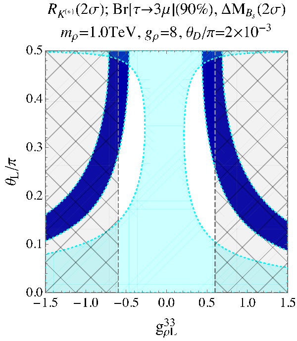
When we try to address the anomalies associated with the currents $b\to s\mu^{+}\mu^{-}$ and $b\to c\tau^{-}\overline{\nu}$ , we should take account of related constraints from $B^{0}_{s}\,(=s\overline{b})\leftrightarrow\overline{B^{0}_{s}}\,(=b\overline{s})$ , $\tau^{-}\to\mu^{-}\mu^{+}\mu^{-}$ , $b\to s\nu\overline{\nu}$ , $\tau\to\mu s\overline{s}$ , and also others. In our setup, $B^{0}_{s}\leftrightarrow\overline{B^{0}_{s}}$ , $\tau^{-}\to\mu^{-}\mu^{+}\mu^{-}$ generate stringent bounds on the parameters, while constraints from the others are weaker.

As a reasonable benchmark, we selected $m_{\rho}$ and $g_{\rho}$ as $1\,\text{TeV}$ and eight. A preferred situation is focused and summarized in Fig. 1, where the down-quark mixing angle $\theta_{D}$ is chosen as a minuscule digit $(2\pi\times 10^{-3})$ to circumvent the tight bound from the $B^{0}_{s}\leftrightarrow\overline{B^{0}_{s}}$ mixing (the FLAG17 result, $f_{B_{s}}\sqrt{\hat{B}_{B_{s}}}=(274\pm 8)$ MeV [68], being adopted as pointed out in [69]). Here we have taken into account the NLO QCD operator running effects. When we focus on the region $(|g_{\rho L}^{33}|,\theta_{L})\simeq(0.6,\pi/2)$ , the $R_{K^{(*)}}$ anomaly can be addressed near the best-fit point.

Also, a fascinating property is found in the present scenario in the $R_{D^{(*)}}$ variables. The setup contains vector-leptoquark-like and $W^{\prime}$ -like vectors, where they can contribute to $R_{D^{(*)}}$ at the leading order. However, the underlying $SU(8)$ global symmetry reduces the contribution in total, which is vanishing in the degenerated limit of CFVs. This gives us a strong prediction on $R_{D^{(*)}}$ that they are very close to those of SM, and it will be checked in future by experiments.

Refer to caption — Figure 1: The region plot in the plane $(g_{\rho L}^{33},\theta_{L})$ with $\theta_{D}/\pi=2\times 10^{-3}$ fixed for $m_{\rho}=1$ TeV and $g_{\rho}=8$ . The current $R_{K^{(*)}}$ anomaly can be explained in the thick-blue region at the 2 $\sigma$ level, while the cyan-shaded area represents the consistent region with the current 90% C.L. upper limit of $\text{Br}[\tau^{-}\to\mu^{-}\mu^{+}\mu^{-}]$ (based on the experiment [70]). The gray-hatched region is out of the 2 $\sigma$ -favored area for $\Delta M_{B_{s}}$ (based on the result [71]). We adopted the target magnitude of relevant Wilson coefficients derived through their global fit in [72].

4 Addressing $K$ anomaly

We move on to the anomaly and associated constraints in the $K$ system. Looking at the flavor texture in Eq.(8), we find that the contributions of CFVs to the $s$ - $d$ transition observables, $\epsilon^{\prime}/\epsilon$ , $K\to\pi\nu{\bar{\nu}}$ and $K^{0}$ - $\bar{K}^{0}$ mixing ( $\Delta M_{K}$ ) are possibly generated. Also, we ought to focus on the $c$ - $u$ transition, where observables in the $D^{0}$ - $\bar{D}^{0}$ mixing provide us additional constraints on the scenario.

First, we focus on the correlation between $\epsilon^{\prime}/\epsilon$ and $K^{0}$ - $\bar{K}^{0}$ mixing ( $\Delta M_{K}$ ). For the $\Delta M_{K}$ , as was prescribed in Ref. [45], we may derive the limit simply by allowing the new physics effect to come within the 2 $\sigma$ uncertainty of the current measurement ( $\Delta M_{K}^{\rm exp}=(3.484\pm 0.006)\times 10^{-15}$ GeV [33]). The concrete digit is $|\Delta M_{K}^{\rm NP}|<3.496\times 10^{-15}\,{\rm GeV}$ (NP: new physics).

The CFV contributions to the direct CP violation in the $K\to\pi\pi$ processes are evaluated at the NLO perturbation in QCD and QED coupling expansions as [34]

\displaystyle\left(\frac{\epsilon^{\prime}}{\epsilon}\right)^{\rm CFVs}

\displaystyle=\frac{\omega_{+}}{\sqrt{2}\left|\epsilon_{K}^{\textrm{exp}}\right|\textrm{Re}A_{0}^{\textrm{exp}}}\langle\vec{Q}_{\epsilon^{\prime}}(\mu)^{T}\rangle\hat{U}\left(\mu,m_{\rho}\right)\textrm{Im}\left[\vec{C}(m_{\rho})\right],

(12)

where $\vec{C}(m_{\rho})=(C_{1}(m_{\rho}),C_{2}(m_{\rho}),C_{3}(m_{\rho}),\cdots,C_{10}(m_{\rho}))^{T}$ shows the vector from of relevant Wilson coefficients (see [55] for details), ${\textrm{Re}}A_{0}^{\textrm{exp}}=(3.3201\pm 0.0018)\times 10^{-7}{\textrm{GeV}}$ [73], and $\omega_{+}|_{\rm SM}\equiv a\,{{\rm Re}A_{2}|_{\rm SM}}/{\rm Re}A_{0}|_{\rm SM}=4.53\times 10^{-2}$ [74, 35]. The coefficients $\langle\vec{Q}_{\epsilon^{\prime}}(\mu)^{T}\rangle\hat{U}\left(\mu,m_{\rho}\right)$ , which denote the evolution of the hadronic matrix elements from the scale $\mu$ to the NP scale $m_{\rho}$ , are given in Ref. [34], where $\langle\vec{Q}_{\epsilon^{\prime}}(\mu)^{T}\rangle$ is defined as

\displaystyle{\langle\vec{Q}_{\epsilon^{\prime}}(\mu)^{T}\rangle\equiv\frac{1}{\omega_{+}}\langle\vec{Q}(\mu)^{T}\rangle_{2}-\langle\vec{Q}(\mu)^{T}\rangle_{0}(1-\hat{\Omega}_{\text{eff}}).}

(13)

The vector forms $\langle\vec{Q}(\mu)^{T}\rangle_{I}\,(I=0,2)$ are defined from $\langle Q_{j}({\mu})\rangle_{I}$ like $\vec{C}(m_{\rho})$ (where the concrete information on $\langle\vec{Q}(\mu)^{T}\rangle_{I}$ and $\hat{U}\left(\mu,m_{\rho}\right)$ are available in [34]). The factors for the isospin breaking correction are described in the matrix form,

\displaystyle{(1-\hat{\Omega}_{\text{eff}})_{ij}=\begin{cases}0.852&(i=j=1-6),\\ 0.983&(i=j=7-10),\\ 0&(i\not=j).\end{cases}}

(14)

Here the scale $\mu$ is set to be $1.3\,\text{GeV}$ . In the LO analysis where $C_{5}(m_{\rho}),C_{6}(m_{\rho})$ and $C_{7}(m_{\rho})$ bring main effects on $C_{6}(m_{c})$ and $C_{8}(m_{c})$ , we found that the contributions from QCD penguin $Q_{6}$ dominates in the $\epsilon^{\prime}/\epsilon$ , and the EW penguin $Q_{8}$ term yields about $60\%$ contribution of them. Fig. 2 tells us that there is an upper bound on $m_{\rho}$ for each choice of $g_{\rho}$ , e.g., $m_{\rho}\lesssim 1.4\,\text{TeV}$ for $g_{\rho}=8$ . For addressing the $(\epsilon^{\prime}/\epsilon)$ anomaly, we need nonzero $\mathcal{V}$ - $\rho$ mixing to generate relevant connections to current interactions, where we remind that $(g_{s,W,Y}/g_{\rho})$ determines the size of the mixing. This property gives us a great hint for pursuing signals of this scenario in experiments.

Second, we go for the summary plot, where the following parameters, $(m_{\rho},g_{\rho},\theta_{L},\theta_{D})$ , are fixed as $(1\,\text{TeV},8,\pi/2,\,2\pi\times 10^{-3}\text{ or }1.5\pi\times 10^{-3})$ , respectively to address the $R_{K^{(*)}}$ anomaly successfully. In addition to $\Delta M_{K}$ , Br[ $K^{+}\to\pi^{+}\nu\bar{\nu}$ ], Br[ $K_{L}\to\pi^{0}\nu\bar{\nu}$ ], and $D^{0}$ - $\bar{D}^{0}$ mixing provide constraints on the scenario. We itemize the relevant aspects of Fig. 3.

•

Since the flavor of the neutrinos is not identified in experiments, the constraints from $K^{+}\to\pi^{+}\nu\bar{\nu}$ and $K_{L}\to\pi^{0}\nu\bar{\nu}$ hold correlations between $g_{\rho L}^{12}$ and $g_{\rho L}^{33}$ .
•

Addressing $R_{K^{(*)}}$ and $\epsilon^{\prime}/\epsilon$ within $1\sigma$ C.L.s looks possible, but it is realizable very in a limited parameter space. If we relax it to $2\sigma$ C.L.s, still we find sufficient regions of parameters.
•

A part of the region where $\epsilon^{\prime}/\epsilon$ can be addressed seems to be excluded by the constraint from the $D^{0}$ - $\bar{D}^{0}$ mixing. Nevertheless, as shown in the left panel of Fig. 3, the $95\%$ C.L. interval highly depends on the choice of the uncertain input $x^{\text{SM}}$ (see [55] for details). Taking account of the uncertainty for $x^{\text{SM}}$ , we can conclude that no definite bound is put on the red vertical domains (for $\epsilon^{\prime}/\epsilon$ ) in Fig. 3.
•

According to the literature [78], by the end of 2018 the NA62 experiment will measure the $K^{+}\to\pi^{+}\nu\bar{\nu}$ with about 10% accuracy of the SM prediction. The KOTO experiment also plans to report new results on the data analysis on the $K_{L}\to\pi^{0}\nu\bar{\nu}$ in the near future, to be expected to reach the level of $<10^{-9}$ for the branching ratio, corresponding to 2015 - 2018 data taking [79]. In the near future, such updated bounds will restrict the relevant parameter regions sizably.

5 Status of LHC dilepton search

Generally, vector particles coupled with a pair of muons are significantly constrained by direct dimuon resonance searches at the LHC. In our scenario, flavor universal couplings to up- and down-quarks dominate production cross section even though the suppression factor $(g_{s}/g_{\rho})$ works. As shown in Fig. 4, the additional widths of the CFVs contributing the production are required to be large as $\Gamma_{\text{add}}/m_{\rho}\sim 30\%$ . Such an additional width would be present when the CFV can dominantly couple to a hidden dark sector including a dark matter candidate, or a pionic sector realized as in a hidden QCD with a setup similar to the present CFV content [65].

6 Summary

In the present setup of chiral-flavorful vectors (CFVs), not only the (assumed) flavor changing interactions, but also the flavor universal interactions through the mixing of the CFVs and the gauge bosons in the standard model (SM) due to manifestly realized SM gauge invariance, play important roles. Under the presence of the latter interactions, we can successfully address the anomaly in $\epsilon^{\prime}/\epsilon$ in the Kaon sector, in addition to the deviations in observables associated with $b\to s\mu^{+}\mu^{-}$ , including $R_{K^{(*)}}$ . Almost vanishing contributions to the variables $R_{D^{(*)}}$ are realized due to remnant of the $SU(8)$ global symmetry, which is a strong prediction of our scenario even though the presently reported excesses in $R_{D^{(*)}}$ cannot be explained. Limited (quite wide) parameter space still remains for a simultaneous explanation of $R_{K^{(*)}}$ and $\epsilon^{\prime}/\epsilon$ within $1\sigma$ ( $2\sigma$ ) C.L. individually. In addition to the LHC direct searches, also the NA62 and KOTO experiments will explore the parameter space for the explanations through measuring Br[ $K^{+}\to\pi^{+}\nu\bar{\nu}$ ] and Br[ $K_{L}\to\pi^{0}\nu\bar{\nu}$ ], respectively.

Note added: In the latter half of March 2019 during the Rencontres de Moriond 2019, the Belle and LHCb experimental groups have published their latest results on the $B$ anomalies, which include

$\displaystyle R_{K^{*}}^{[0.045,1.1]}$	$\displaystyle=0.52^{+0.36}_{-0.26}\pm 0.05,$	$\displaystyle\text{(Belle)~\cite[cite]{[\@@bibref{}{Belle-RK-Moriond2019}{}{}]}},$	(15)
$\displaystyle R_{K^{*}}^{[1.1,6]}$	$\displaystyle=0.96^{+0.45}_{-0.29}\pm 0.11,$	$\displaystyle\text{(Belle)~\cite[cite]{[\@@bibref{}{Belle-RK-Moriond2019}{}{}]}},$	(16)
$\displaystyle R_{K}^{[1.1,6]}$	$\displaystyle=0.846^{+0.060+0.016}_{-0.054-0.014},$	$\displaystyle\text{(LHCb)~\cite[cite]{[\@@bibref{}{LHCb-RK-Moriond2019}{}{}]}},$	(17)
$\displaystyle R_{D}$	$\displaystyle=0.307\pm 0.037\pm 0.016,$	$\displaystyle\text{(Belle)~\cite[cite]{[\@@bibref{}{Belle-RD-Moriond2019}{}{}]}},$	(18)
$\displaystyle R_{D{*}}$	$\displaystyle=0.283\pm 0.018\pm 0.014,$	$\displaystyle\text{(Belle)~\cite[cite]{[\@@bibref{}{Belle-RD-Moriond2019}{}{}]}}.$	(19)

The LHCb group announced that their updated result on $R_{K}$ by use of $2011$ , $2012$ , $2015$ and $2016$ data becomes $\sim 2.5\,\sigma$ from the SM (previously $\sim 2.6\,\sigma$ using $2011$ and $2012$ data), while the Belle group claimed that the $R_{D}$ - $R_{D^{*}}$ experimental world average of the deviation is decreased to $3.1\,\sigma$ from $3.8\,\sigma$ . These results implies that both of the $R_{K^{(*)}}$ and $R_{D^{(*)}}$ anomalies may become ‘less significant’. Nevertheless, sizable deviations can remains, and then the discussion on this manuscript is basically still valid.

Acknowledgements

The presenter (K.N.) would like to thank the organizers for kind invitation and hospitalities during the workshop.

References

[1] S. Descotes-Genon, T. Hurth, J. Matias and J. Virto, JHEP 1305, 137 (2013) doi:10.1007/JHEP05(2013)137 [arXiv:1303.5794 [hep-ph]].
[2] S. Descotes-Genon, J. Matias and J. Virto, Phys. Rev. D 88, 074002 (2013) doi:10.1103/PhysRevD.88.074002 [arXiv:1307.5683 [hep-ph]].
[3] W. Altmannshofer and D. M. Straub, Eur. Phys. J. C 73, 2646 (2013) doi:10.1140/epjc/s10052-013-2646-9 [arXiv:1308.1501 [hep-ph]].
[4] G. Hiller and M. Schmaltz, Phys. Rev. D 90, 054014 (2014) doi:10.1103/PhysRevD.90.054014 [arXiv:1408.1627 [hep-ph]].
[5] W. Altmannshofer and D. M. Straub, Eur. Phys. J. C 75, no. 8, 382 (2015) doi:10.1140/epjc/s10052-015-3602-7 [arXiv:1411.3161 [hep-ph]].
[6] A. Datta, M. Duraisamy and D. Ghosh, Phys. Rev. D 86, 034027 (2012) doi:10.1103/PhysRevD.86.034027 [arXiv:1206.3760 [hep-ph]].
[7] A. Celis, M. Jung, X. Q. Li and A. Pich, JHEP 1301, 054 (2013) doi:10.1007/JHEP01(2013)054 [arXiv:1210.8443 [hep-ph]].
[8] A. Crivellin, A. Kokulu and C. Greub, Phys. Rev. D 87, no. 9, 094031 (2013) doi:10.1103/PhysRevD.87.094031 [arXiv:1303.5877 [hep-ph]].
[9] I. Doršner, S. Fajfer, N. Košnik and I. Nišandžić, JHEP 1311, 084 (2013) doi:10.1007/JHEP11(2013)084 [arXiv:1306.6493 [hep-ph]].
[10] Y. Sakaki, M. Tanaka, A. Tayduganov and R. Watanabe, Phys. Rev. D 88, no. 9, 094012 (2013) doi:10.1103/PhysRevD.88.094012 [arXiv:1309.0301 [hep-ph]].
[11] P. Biancofiore, P. Colangelo and F. De Fazio, Phys. Rev. D 89, no. 9, 095018 (2014) doi:10.1103/PhysRevD.89.095018 [arXiv:1403.2944 [hep-ph]].
[12] C. Niehoff, P. Stangl and D. M. Straub, Phys. Lett. B 747, 182 (2015) doi:10.1016/j.physletb.2015.05.063 [arXiv:1503.03865 [hep-ph]].
[13] C. Niehoff, P. Stangl and D. M. Straub, JHEP 1601, 119 (2016) doi:10.1007/JHEP01(2016)119 [arXiv:1508.00569 [hep-ph]].
[14] A. Carmona and F. Goertz, Phys. Rev. Lett. 116, no. 25, 251801 (2016) doi:10.1103/PhysRevLett.116.251801 [arXiv:1510.07658 [hep-ph]].
[15] R. Barbieri, G. Isidori, A. Pattori and F. Senia, Eur. Phys. J. C 76, no. 2, 67 (2016) doi:10.1140/epjc/s10052-016-3905-3 [arXiv:1512.01560 [hep-ph]].
[16] E. Megias, G. Panico, O. Pujolas and M. Quiros, JHEP 1609, 118 (2016) doi:10.1007/JHEP09(2016)118 [arXiv:1608.02362 [hep-ph]].
[17] R. Barbieri, C. W. Murphy and F. Senia, Eur. Phys. J. C 77, no. 1, 8 (2017) doi:10.1140/epjc/s10052-016-4578-7 [arXiv:1611.04930 [hep-ph]].
[18] E. Megias, M. Quiros and L. Salas, JHEP 1707, 102 (2017) doi:10.1007/JHEP07(2017)102 [arXiv:1703.06019 [hep-ph]].
[19] D. Buttazzo, A. Greljo, G. Isidori and D. Marzocca, JHEP 1711, 044 (2017) doi:10.1007/JHEP11(2017)044 [arXiv:1706.07808 [hep-ph]].
[20] E. Megias, M. Quiros and L. Salas, Phys. Rev. D 96, no. 7, 075030 (2017) doi:10.1103/PhysRevD.96.075030 [arXiv:1707.08014 [hep-ph]].
[21] J. M. Cline, Phys. Rev. D 97, no. 1, 015013 (2018) doi:10.1103/PhysRevD.97.015013 [arXiv:1710.02140 [hep-ph]].
[22] M. Bordone, C. Cornella, J. Fuentes-Martin and G. Isidori, Phys. Lett. B 779, 317 (2018) doi:10.1016/j.physletb.2018.02.011 [arXiv:1712.01368 [hep-ph]].
[23] G. D’Ambrosio and A. M. Iyer, Eur. Phys. J. C 78, no. 6, 448 (2018) doi:10.1140/epjc/s10052-018-5915-9 [arXiv:1712.08122 [hep-ph]].
[24] M. Blanke and A. Crivellin, Phys. Rev. Lett. 121, no. 1, 011801 (2018) doi:10.1103/PhysRevLett.121.011801 [arXiv:1801.07256 [hep-ph]].
[25] M. Bordone, C. Cornella, J. Fuentes-Martín and G. Isidori, JHEP 1810, 148 (2018) doi:10.1007/JHEP10(2018)148 [arXiv:1805.09328 [hep-ph]].
[26] A. Crivellin, C. Greub, D. Müller and F. Saturnino, Phys. Rev. Lett. 122, no. 1, 011805 (2019) doi:10.1103/PhysRevLett.122.011805 [arXiv:1807.02068 [hep-ph]].
[27] J. Aebischer, A. Crivellin and C. Greub, Phys. Rev. D 99, no. 5, 055002 (2019) doi:10.1103/PhysRevD.99.055002 [arXiv:1811.08907 [hep-ph]].
[28] R. Watanabe, Phys. Lett. B 776, 5 (2018) doi:10.1016/j.physletb.2017.11.016 [arXiv:1709.08644 [hep-ph]].
[29] R. Aaij et al. [LHCb Collaboration], Phys. Rev. Lett. 120, no. 12, 121801 (2018) doi:10.1103/PhysRevLett.120.121801 [arXiv:1711.05623 [hep-ex]].
[30] J. R. Batley et al. [NA48 Collaboration], Phys. Lett. B 544, 97 (2002) doi:10.1016/S0370-2693(02)02476-0 [hep-ex/0208009].
[31] A. Alavi-Harati et al. [KTeV Collaboration], Phys. Rev. D 67, 012005 (2003) Erratum: [Phys. Rev. D 70, 079904 (2004)] doi:10.1103/PhysRevD.70.079904, 10.1103/PhysRevD.67.012005 [hep-ex/0208007].
[32] E. Abouzaid et al. [KTeV Collaboration], Phys. Rev. D 83, 092001 (2011) doi:10.1103/PhysRevD.83.092001 [arXiv:1011.0127 [hep-ex]].
[33] M. Tanabashi et al. [Particle Data Group], Phys. Rev. D 98, no. 3, 030001 (2018). doi:10.1103/PhysRevD.98.030001
[34] T. Kitahara, U. Nierste and P. Tremper, JHEP 1612, 078 (2016) doi:10.1007/JHEP12(2016)078 [arXiv:1607.06727 [hep-ph]].
[35] A. J. Buras, M. Gorbahn, S. Jäger and M. Jamin, JHEP 1511, 202 (2015) doi:10.1007/JHEP11(2015)202 [arXiv:1507.06345 [hep-ph]].
[36] Z. Bai et al. [RBC and UKQCD Collaborations], Phys. Rev. Lett. 115, no. 21, 212001 (2015) doi:10.1103/PhysRevLett.115.212001 [arXiv:1505.07863 [hep-lat]].
[37] M. Blanke, A. J. Buras and S. Recksiegel, Eur. Phys. J. C 76, no. 4, 182 (2016) doi:10.1140/epjc/s10052-016-4019-7 [arXiv:1507.06316 [hep-ph]].
[38] A. J. Buras and J. M. Gérard, JHEP 1512, 008 (2015) doi:10.1007/JHEP12(2015)008 [arXiv:1507.06326 [hep-ph]].
[39] A. J. Buras and F. De Fazio, JHEP 1603, 010 (2016) doi:10.1007/JHEP03(2016)010 [arXiv:1512.02869 [hep-ph]].
[40] A. J. Buras and J. M. Gerard, Eur. Phys. J. C 77, no. 1, 10 (2017) doi:10.1140/epjc/s10052-016-4586-7 [arXiv:1603.05686 [hep-ph]].
[41] M. Tanimoto and K. Yamamoto, PTEP 2016, no. 12, 123B02 (2016) doi:10.1093/ptep/ptw160 [arXiv:1603.07960 [hep-ph]].
[42] T. Kitahara, U. Nierste and P. Tremper, Phys. Rev. Lett. 117, no. 9, 091802 (2016) doi:10.1103/PhysRevLett.117.091802 [arXiv:1604.07400 [hep-ph]].
[43] M. Endo, S. Mishima, D. Ueda and K. Yamamoto, Phys. Lett. B 762, 493 (2016) doi:10.1016/j.physletb.2016.10.009 [arXiv:1608.01444 [hep-ph]].
[44] C. Bobeth, A. J. Buras, A. Celis and M. Jung, JHEP 1704, 079 (2017) doi:10.1007/JHEP04(2017)079 [arXiv:1609.04783 [hep-ph]].
[45] M. Endo, T. Kitahara, S. Mishima and K. Yamamoto, Phys. Lett. B 771, 37 (2017) doi:10.1016/j.physletb.2017.05.026 [arXiv:1612.08839 [hep-ph]].
[46] A. Crivellin, G. D’Ambrosio, T. Kitahara and U. Nierste, Phys. Rev. D 96, no. 1, 015023 (2017) doi:10.1103/PhysRevD.96.015023 [arXiv:1703.05786 [hep-ph]].
[47] V. Chobanova, G. D’Ambrosio, T. Kitahara, M. Lucio Martinez, D. Martinez Santos, I. S. Fernandez and K. Yamamoto, JHEP 1805, 024 (2018) doi:10.1007/JHEP05(2018)024 [arXiv:1711.11030 [hep-ph]].
[48] M. Endo, T. Goto, T. Kitahara, S. Mishima, D. Ueda and K. Yamamoto, JHEP 1804, 019 (2018) doi:10.1007/JHEP04(2018)019 [arXiv:1712.04959 [hep-ph]].
[49] C. Bobeth and A. J. Buras, JHEP 1802, 101 (2018) doi:10.1007/JHEP02(2018)101 [arXiv:1712.01295 [hep-ph]].
[50] H. Gisbert and A. Pich, Rept. Prog. Phys. 81, no. 7, 076201 (2018) doi:10.1088/1361-6633/aac18e [arXiv:1712.06147 [hep-ph]].
[51] N. Haba, H. Umeeda and T. Yamada, JHEP 1805, 052 (2018) doi:10.1007/JHEP05(2018)052 [arXiv:1802.09903 [hep-ph]].
[52] C. H. Chen and T. Nomura, JHEP 1808, 145 (2018) doi:10.1007/JHEP08(2018)145 [arXiv:1804.06017 [hep-ph]].
[53] C. H. Chen and T. Nomura, Phys. Lett. B 787, 182 (2018) doi:10.1016/j.physletb.2018.11.006 [arXiv:1805.07522 [hep-ph]].
[54] A. J. Buras, Acta Phys. Polon. B 49, 1043 (2018) doi:10.5506/APhysPolB.49.1043 [arXiv:1805.11096 [hep-ph]].
[55] S. Matsuzaki, K. Nishiwaki and K. Yamamoto, JHEP 1811, 164 (2018) doi:10.1007/JHEP11(2018)164 [arXiv:1806.02312 [hep-ph]].
[56] N. Haba, H. Umeeda and T. Yamada, JHEP 1810, 006 (2018) doi:10.1007/JHEP10(2018)006 [arXiv:1806.03424 [hep-ph]].
[57] J. Aebischer, A. J. Buras and J. M. Gérard, JHEP 1902, 021 (2019) doi:10.1007/JHEP02(2019)021 [arXiv:1807.01709 [hep-ph]].
[58] J. Aebischer, C. Bobeth, A. J. Buras, J. M. Gérard and D. M. Straub, arXiv:1807.02520 [hep-ph].
[59] J. Aebischer, C. Bobeth, A. J. Buras and D. M. Straub, Eur. Phys. J. C 79, no. 3, 219 (2019) doi:10.1140/epjc/s10052-019-6715-6 [arXiv:1808.00466 [hep-ph]].
[60] C. H. Chen and T. Nomura, JHEP 1903, 009 (2019) doi:10.1007/JHEP03(2019)009 [arXiv:1808.04097 [hep-ph]].
[61] C. H. Chen and T. Nomura, arXiv:1811.02315 [hep-ph].
[62] C. H. Chen and T. Nomura, arXiv:1812.05904 [hep-ph].
[63] A. J. Buras, arXiv:1812.06102 [hep-ph].
[64] C. Marzo, L. Marzola and M. Raidal, arXiv:1901.08290 [hep-ph].
[65] S. Matsuzaki, K. Nishiwaki and R. Watanabe, JHEP 1708, 145 (2017) doi:10.1007/JHEP08(2017)145 [arXiv:1706.01463 [hep-ph]].
[66] A. J. Buras, JHEP 1604, 071 (2016) doi:10.1007/JHEP04(2016)071 [arXiv:1601.00005 [hep-ph]].
[67] B. Bhattacharya, A. Datta, J. P. Guévin, D. London and R. Watanabe, JHEP 1701, 015 (2017) doi:10.1007/JHEP01(2017)015 [arXiv:1609.09078 [hep-ph]].
[68] S. Aoki et al., Eur. Phys. J. C 77, no. 2, 112 (2017) doi:10.1140/epjc/s10052-016-4509-7 [arXiv:1607.00299 [hep-lat]].
[69] L. Di Luzio, M. Kirk and A. Lenz, Phys. Rev. D 97, no. 9, 095035 (2018) doi:10.1103/PhysRevD.97.095035 [arXiv:1712.06572 [hep-ph]].
[70] K. Hayasaka et al., Phys. Lett. B 687, 139 (2010) doi:10.1016/j.physletb.2010.03.037 [arXiv:1001.3221 [hep-ex]].
[71] Y. Amhis et al. [Heavy Flavor Averaging Group (HFAG)], arXiv:1412.7515 [hep-ex].
[72] B. Capdevila, A. Crivellin, S. Descotes-Genon, J. Matias and J. Virto, JHEP 1801, 093 (2018) doi:10.1007/JHEP01(2018)093 [arXiv:1704.05340 [hep-ph]].
[73] T. Blum et al., Phys. Rev. D 91, no. 7, 074502 (2015) doi:10.1103/PhysRevD.91.074502 [arXiv:1502.00263 [hep-lat]].
[74] V. Cirigliano, G. Ecker, H. Neufeld and A. Pich, Eur. Phys. J. C 33, 369 (2004) doi:10.1140/epjc/s2003-01579-3 [hep-ph/0310351].
[75] A. V. Artamonov et al. [E949 Collaboration], Phys. Rev. Lett. 101, 191802 (2008) doi:10.1103/PhysRevLett.101.191802 [arXiv:0808.2459 [hep-ex]].
[76] J. K. Ahn et al. [E391a Collaboration], Phys. Rev. D 81, 072004 (2010) doi:10.1103/PhysRevD.81.072004 [arXiv:0911.4789 [hep-ex]].
[77] J. K. Ahn et al. [KOTO Collaboration], Phys. Rev. Lett. 122, no. 2, 021802 (2019) doi:10.1103/PhysRevLett.122.021802 [arXiv:1810.09655 [hep-ex]].
[78] S. Wehle, S. Yaschenko, C. Niebuhr and A. Ishikawa, Private communication, tech. rep., 2017.
[79] Y. Nomura, “Status of KOTO experiment: $K_{L}\to\pi^{0}\nu\bar{\nu}$ at J-PARC, Talk at Heavy Quarks and Leptons 2018.”
[80] The ATLAS collaboration [ATLAS Collaboration], ATLAS-CONF-2017-027.
[81] J. Pumplin, D. R. Stump, J. Huston, H. L. Lai, P. M. Nadolsky and W. K. Tung, JHEP 0207, 012 (2002) doi:10.1088/1126-6708/2002/07/012 [hep-ph/0201195].
[82] D. B. Clark, E. Godat and F. I. Olness, Comput. Phys. Commun. 216, 126 (2017) doi:10.1016/j.cpc.2017.03.004 [arXiv:1605.08012 [hep-ph]].
[83] T. Hahn, Comput. Phys. Commun. 168, 78 (2005) doi:10.1016/j.cpc.2005.01.010 [hep-ph/0404043].
[84] Markus Prim on behalf of the Belle collaboration, “Search for $B\to\ell\nu\gamma$ and $B\to\mu\nu_{\mu}$ and Test of Lepton Universality with $R(K^{\ast})$ at Belle,” Talk at Rencontres de Moriond 2019, Electroweak Interactions and Unified Theories.
[85] Thibaud Humair on behalf of the LHCb collaboration, “Lepton Flavor Universality tests with heavy flavour decays at LHCb,” Talk at Recontres de Moriond 2019, Electroweak Interactions and Unified Theories.
[86] Giacomo Caria on behalf of the Belle collaboration, “Measurement of $R(D)$ and $R(D^{\ast})$ with a semileptonic tag at Belle,” Talk at Rencontres de Moriond 2019, Electroweak Interactions and Unified Theories.

Simultaneous explanation of KK and BB anomalies in vectorlike compositeness