Nonlinear atom-plasmon interactions enabled by nanostructured graphene

Precise control over light-matter interactions on nanometric length scales presents opportunities in technologies such as light energy harvesting Atwater and Polman 2010, optical biosensing Fabrizio et al. 2016, and quantum information Lodahl et al. 2015. Plasmons, consisting of electromagnetic fields hybridized with collective charge-carrier oscillations, are ideal for this purpose, as they couple strongly with impinging light and can focus it into nanoscale volumes Maier 2007; Schuller et al. 2010. The interaction of enhanced local fields produced by resonantly illuminated plasmonic nanostructures with quantum emitters (QEs), such as atoms or molecules (natural or artificial), is of particular interest to the quantum optics and optical sensing communities Achermann 2010; Brolo 2012; Koenderink 2017. Typically, optimal coupling is achieved by engineering the geometry of a noble metal nanostructure so that a plasmon resonates with an electronic transition in a proximal dipole emitter (e.g., an exciton in a quantum dot). However, because noble metal plasmons cannot easily be modified using external stimuli Brown et al. 2015, resonant light-matter interactions in noble metal-QE nanocomposites typically lack the active tunability required by many photonic device functionalities, and are further hindered by large intrinsic Ohmic losses Khurgin 2015.

In its pristine form, graphene, the atomically thin carbon layer, is a zero-gap semiconductor that presents broadband 2.3% optical absorption from transitions between linear valence and conduction bands Castro Neto et al. 2009. When doped to a Fermi energy ${E_{\rm F}}$, Pauli blocking prohibits vertical interband absorption for photon energies $\hbar\omega\leq 2{E_{\rm F}}$, and graphene plasmons, consisting of coherently-coupled virtual intraband transitions, emerge within this gap. These resonances exhibit stronger confinement and longer lifetimes than their noble metal counterparts, and are readily tuned in an active manner via electrostatic gating Grigorenko et al. 2012. For these reasons, the interaction of plasmonic near fields from highly doped graphene with proximal QEs has been predicted to enable observable vacuum Rabi splittings Koppens et al. 2011, large Purcell enhancement factors Nikitin et al. 2011; Sloan et al. 2018, and electrical control of quantum states Manjavacas et al. 2012. Unfortunately, even at high doping levels, plasmon energies $\hbar\omega_{\rm p}$ in graphene nanostructures appear in the infrared or terahertz regimes, well-below the frequencies associated with long-lived electronic excitations in robust quantum light sources. Indeed, graphene structures with a characteristic size $D$ exhibit localized plasmons at energies scaling like $\hbar\omega_{\rm p}\propto\sqrt{{E_{\rm F}}/D}$, which for achievable values of ${E_{\rm F}}<1$ eV and $D>10$ nm have so far been demonstrated at mid-infrared and lower frequencies. Additionally, coupling to optical phonons persists as a strong source of damping for plasmons at energies above $\sim 0.2$ eV Yan et al. 2013, as do interband transitions unless $\hbar\omega_{\rm p}\lesssim{E_{\rm F}}$ García de Abajo 2014.

The conical electronic dispersion of graphene imposes anharmonic intraband charge-carrier motion, resulting in an intrinsically nonlinear response to external electromagnetic fields, including efficient generation of odd-ordered harmonics Mikhailov 2007; Ishikawa 2010; Cheng et al. 2015; Mikhailov 2016; Jiang et al. 2018; Soavil et al. 2018; Hafez et al. 2018. The synergistic combination of a large optical nonlinearity and strong plasmonic near-field enhancement, both arising from intraband transitions in doped graphene, is currently motivating intensive research efforts in the emerging field of nonlinear graphene plasmonics Cox and García de Abajo 2014; Jablan and Chang 2015; Christensen et al. 2015; Constant et al. 2016; Jadidi et al. 2016; Cox et al. 2017a; Cox et al. 2017b; Kundys et al. 2018. In particular, 2D plasmons in graphene nanostructures have been predicted to generate harmonics with efficiency above that of similarly sized noble metal nanostructures Cox and García de Abajo 2014.

In this work, we propose to harness plasmon-enhanced harmonic generation in nanostructured graphene to couple the 2D material with a nearby QE, effectively bridging the energy mismatch between the electrically tunable infrared graphene plasmon and a near-infrared excitation in the emitter. We show that resonant excitation of a localized graphene plasmon can reduce the impinging light intensity required to generate a substantial third-harmonic (TH) near field, which can be actively tuned to the desired emitter resonance frequency by exploiting the unique electro-optic response of graphene. For the realistic parameters considered in this work, our simulations predict strong nonlinear plasmonic interactions that can drive fluorescence in two-level atoms and electromagnetically induced transparency (EIT) or coherent population control in three-level QEs. The present nonlinear coupling strategy can be used generally to probe nonlinear plasmonic near fields Metzger et al. 2017; Yang et al. 2017, while the electrical tunability of graphene plasmons can be exploited to control single-photon emission and actively manipulate quantum states.

A prototypical hybrid molecule consists of a doped graphene nanodisk with diameter $D=40$ nm and a two-level QE located a distance $d$ directly above its center, the latter characterized by the dipole moment $\vec{\mu}_{12}$ associated with the transition between states $\ket{1}$ and $\ket{2}$, which we consider to be oriented parallel to the graphene plane with magnitude $1\,e\times$ nm ($\sim 50$ Debye, commensurate with quantum dot excitons Stievater et al. 2001). We consider local, isotropic dielectric media above and below the graphene layer characterized by the permittivities $\epsilon^{\rm a}_{\omega}$ and $\epsilon^{\rm b}_{\omega}$, respectively. As illustrated schematically in Fig. 1(a), an impinging light electric field ${\bf E}_{\rm ext}$ with frequency $\omega\approx\omega_{\rm p}$ (red beam) generates a plasmon-enhanced TH near-field, ${\bf E}^{33}_{\rm ind}({\bf r},\omega)\text{e}^{-\text{i}3\omega t}+{\rm c.c.}$, around the nanodisk (blue field), which we describe semianalytically by adopting a classical electrostatic eigenmode decomposition (see Ref. Cox et al. 2017b and Appendix). Electron dynamics in the QE is governed by the density matrix master equation,

where $\mathcal{H}$ is the system Hamiltonian and $\mathcal{L}[\rho]$ denotes the Lindblad superoperator accounting for decoherence. For a two-level system we write the Hamiltonian

with $\hbar\varepsilon_{j}$ denoting the energy of the QE state $\ket{j}$. Defining the slowly-varying coherence elements $\tilde{\rho}_{12}=\rho_{12}\text{e}^{\text{i}3\omega t}$ and $\tilde{\rho}_{21}=\rho_{21}\text{e}^{-\text{i}3\omega t}$, we write the average QE transition dipole moment as ${\bf d}(t)=\vec{\mu}_{12}(\tilde{\rho}_{21}\text{e}^{\text{i}3\omega t}+\tilde{\rho}_{12}\text{e}^{-\text{i}3\omega t})$. Then, inserting Eq. (2) into Eq. (1) and using the expressions for $\mathcal{L}[\rho]$ and ${\bf E}^{33}_{\rm ind}$ provided in the Appendix, the density matrix equations of motion in the rotating-wave approximation are found to be

where we adopt $\Gamma_{0}=1$ ns^-1 as a phenomenological relaxation rate from the excited state $\ket{2}$ to the ground state $\ket{1}$, $\Delta\equiv 3\omega-\varepsilon_{12}$ is the detuning of the TH near-field from the QE resonance energy $\hbar\varepsilon_{12}\equiv\hbar\varepsilon_{2}-\hbar\varepsilon_{1}$,

is the Rabi frequency quantifying the direct coupling of the QE with the TH near-field produced by the 2D nanostructure, and

characterizes the self-interaction strength of the induced QE dipole at frequency $s\omega$ enabled by graphene. In the above expressions,

denotes the normalized electric field produced at ${\bf r}=(0,0,d)$ by integrating the so-called plasmon wave function (see Ref. Yu et al. 2017a and Appendix) $\rho_{m}({\bf R})$ associated with mode $m$ over the 2D position vector ${\bf R}$ within the graphene nanostructure. The dimensionless parameters $\eta^{(1)}_{s\omega}\equiv 2\text{i}\sigma^{(1)}_{s\omega}/{s\omega}D(\epsilon^{\rm a}_{s\omega}+\epsilon^{\rm b}_{s\omega})$ in Eqs. (4) and (5), containing the dependence on the linear conductivities of extended graphene $\sigma^{(1)}_{s\omega}$ at frequency ${s\omega}$ (calculated in the local limit of the random-phase approximation García de Abajo 2014; Wunsch et al. 2006), yield resonant spectral features in $\Omega$ and $G$ at frequencies ${s\omega}$ satisfying ${\rm Re}\{\eta^{(1)}_{s\omega}/\eta_{m}\}=1$, where $\eta_{m}$ are modal eigenvalues, with strengths determined by the corresponding dipolar coupling parameters $\vec{\xi}_{m}=\int d^{2}{\bf R}{\bf R}\rho_{m}({\bf R})/D^{3}$. TH generation is characterized by the local third-order conductivity of extended graphene $\sigma^{(3)}_{3\omega}$, for which we adopt the analytical result reported in Ref. Mikhailov 2016, obtained quantum-mechanically in the Dirac cone approximation, while $\zeta^{(3)}$ is a third-order coupling parameter (see Appendix). The conductivities employed here, accounting for both interband and intraband electronic transitions in extended graphene at zero temperature, combined with tabulated values of $\eta_{m}$, $\vec{\xi}_{m}$, and $\zeta^{(3)}$, can faithfully reproduce the linear and nonlinear polarizabilities of graphene nanostructures with sizes $\gtrsim 10$ nm predicted in fully-atomistic simulations Cox et al. 2017b.

Nonlinear plasmonic near-field coupling between the nanodisk and QE occurs when the transition energy $\hbar\varepsilon_{12}$ and the plasmon energy $\hbar\omega_{\rm p}$ satisfy $\varepsilon_{12}\approx 3\omega_{\rm p}$, as indicated in Fig. 1(b). The QE undergoes Rabi oscillations at a frequency $\Omega$, while the real and imaginary parts of $G$ contribute to a transition energy renormalization and decay rate enhancement, respectively Zhang et al. 2006; Malyshev and Malyshev 2011; Antón et al. 2012. Using plasmon wave functions and eigenvalues tabulated in Ref. Yu et al. 2017b for a disk geometry, we plot $\Omega$ and $G$ in Figs. 1(c) and 1(d), respectively, for a linearly polarized field parallel to $\vec{\mu}_{12}$ impinging on the QE-nanodisk system in vacuum ($\epsilon^{\rm a}_{\omega}=\epsilon^{\rm b}_{\omega}=1$). With realistic graphene parameters (Fermi energy ${E_{\rm F}}\approx 0.3$–0.7 eV and $66$ fs plasmon lifetime, used throughout this work), a modest separation $d=20$ nm yields Rabi frequencies $\Omega\gtrsim\Gamma_{0}$, indicating strong driving of the QE via plasmon-assisted TH generation. Figures 1(c) and 1(d) show that the atom-plasmon interaction at the TH can be electrically tuned over a larger range of higher frequencies otherwise obtained though linear coupling at the fundamental frequency, while strong transition energy shifts (Re{G}) and decay rate enhancement (Im{G}) associated with $\omega_{\rm p}$ (e.g., in a linear coupling scheme) are avoided at the TH, where only weakly interacting, higher-order plasmon modes play a role.

For the system considered in Fig. 1 under continuous-wave (cw) illumination, we simulate the QE power absorption $P_{\rm abs}=\Gamma_{0}\hbar\varepsilon_{12}\rho_{22}$ from the graphene plasmon TH near-field by examining the steady-state density matrix obtained upon numerical integration of Eqs. (3). In Fig. 2(a) we plot the TH power absorption as a function of the impinging light frequency for different QE-graphene separation distances $d$ (upper panel) and light intensities $I_{\rm ext}$ (lower panel), maintaining ${E_{\rm F}}=0.5$ eV in graphene such that $\hbar\omega_{\rm p}=0.2694$ eV [see Fig. 1(c)] and $\varepsilon_{12}=3\omega_{\rm p}$. Under these conditions, the QE resonance does not interact directly with a plasmon mode of the graphene nanodisk, although a persisting self-interaction at the QE transition frequency, quantified by the parameter $G$, leads to enhanced decay rates and renormalized energies Zhang et al. 2006: this interaction is proportional to the square of the dipole coupling $\vec{\mu}_{12}\cdot{\bf e}_{m}$ [see Eq. (5)] and yields a blue-shifted and broadened power absorption peak at small separations (e.g., $d=10$ nm) but rapidly disappears with increasing separation distance, while the direct TH near-field interaction, which depends linearly on the dipole coupling, diminishes more slowly. In the present nonlinear plasmonic coupling scheme, the TH near-field enhancement of the QE excitation rate ($\Omega$) is independent of the self-interaction strength ($G$), unlike in the degenerate plasmon-exciton coupling scheme, where these competing phenomena are both maximized at the plasmon resonance frequency Doeleman et al. 2016; Koenderink 2017. Under strong driving fields, the TH near-field produces a clear signature of power broadening in the QE absorption spectrum Boyd 2008, leading towards optical bistability and hysteresis fueled by the QE self-interaction Malyshev and Malyshev 2011. In Fig. 2(b) we consider a situation where the illumination frequency is fixed at $\omega=\omega_{\rm p}=\varepsilon_{12}/3$ and the TH power absorption is actively controlled by tuning the Fermi energy ${E_{\rm F}}$ (doping charge density) in the graphene nanodisk.

The effective absorption cross-section of the hybrid system, defined as $P_{\rm abs}/I_{\rm ext}$, can reach values of approximately $\sim 0.06$ nm² (for $I_{\rm ext}=1$ GW/m² at $d=15$ nm), which is several orders of magnitude larger than the optimal cross-section of the dipole emitter in free space, $8\pi\mu_{12}^{2}\varepsilon_{12}/\hbar\Gamma_{0}c\approx 2.5\times 10^{-5}$ nm², but significantly less than the geometrical area of the graphene nanodisk. We further remark that although these results are obtained for intense cw illumination, approaching the damage threshold for graphene, qualitatively similar behavior is expected for pulses of similar peak intensity and durations of several nanoseconds (i.e., with energy densities falling well-below the damage threshold Krauss et al. 2009; Currie et al. 2011; Roberts et al. 2011; Kiisk et al. 2013).

The near-field produced by plasmon-assisted TH generation can be probed in an alternative manner by QEs with more complicated energy-level structures. In a three-level V-type atom, which we study in Fig. 3, EIT Fleischhauer et al. 2005 produces a dip in the absorption associated with one atomic transition when the other is coupled strongly to the TH near-field. This process is illustrated schematically in Fig. 3(a), where two external fields are applied to the hybrid system and the ground state $\ket{1}$ is coupled to two higher-energy states $\ket{2}$ and $\ket{3}$: we consider $\varepsilon_{12}=3\omega_{\rm p}$, while the energy associated with the transition $\ket{1}\leftrightarrow\ket{3}$ is arbitrarily far away from any prominent features in the nanodisk spectrum [see Fig. 3(b)]. By probing the $\ket{1}\leftrightarrow\ket{3}$ transition with a weak field ($\Omega_{\rm probe}=0.01\Gamma_{0}$) while resonantly coupling the $\ket{1}\leftrightarrow\ket{2}$ transition with the TH near-field (i.e., $\omega=\omega_{\rm p}=\varepsilon_{12}/3$), an absorption dip at resonance is observed when the QE and graphene nanodisk are in close proximity and/or the graphene plasmon is strongly driven [see Fig. 3(c)]. The active tunability of the graphene plasmon resonance can be exploited to actively switch EIT on and off, as we demonstrate in Fig. 3(d).

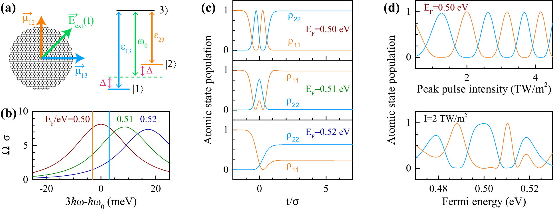
In Fig. 4 we seek to achieve electrical control of atomic state populations using the graphene nanodisk TH near-field. In this scenario, a QE with a lambda-type energy level configuration is located above the nanodisk and has orthogonal dipole moments associated with nearly-degenerate $\ket{1}\leftrightarrow\ket{2}$ and $\ket{2}\leftrightarrow\ket{3}$ transitions [we assume $\Delta=1$ meV; see Fig. 4(a)], which can be simultaneously driven by an optical pulse polarized $45^{\circ}$ from each of them Antón et al. 2012. We consider a Fourier-transform-limited Gaussian pulse of FWHM duration $\sigma=130$ fs, peak intensity $I_{\rm max}$, and carrier frequency $\omega$, such that $3\omega$ is $\pm\Delta$ away from $\varepsilon_{12}$ and $\varepsilon_{13}$, respectively. The effective maximum TH Rabi frequency $\mathinner{\!\left\lvert\Omega\right\rvert}$ for cw light at the peak pulse intensity is plotted in Fig. 4(b) for various Fermi energies, with the energies $\hbar\varepsilon_{12}/3$ and $\hbar\varepsilon_{13}/3$ indicated by vertical lines. Clearly, an asymmetry in the Rabi frequency driving the two nearly degenerate transitions can be introduced by modifying the Fermi energy, resulting in different levels of population transfer from the state $\ket{2}$ to state $\ket{3}$ [Fig. 4(c,d)].

In conclusion, we have demonstrated that plasmon-assisted up-conversion in graphene nanostructures can be used to resonantly excite a proximal QE, enabling energy transfer, EIT, or quantum state population control that would otherwise be prevented by the energy mismatch between infrared graphene plasmons and higher-energy electronic transitions in QEs. This scheme can also be used to probe the nonlinear optical response associated with graphene plasmons, potentially alleviating the sparsity of experimental work in the field of nonlinear graphene plasmonics. While the combination of an intrinsically-large nonlinear response and intense in-plane electric field enhancement associated with localized electrically tunable plasmons renders graphene an ideal material platform for nonlinear near-field coupling, this principle could be straightforwardly applied to other plasmonic materials. We anticipate that the strategy presented here can be used to couple electrically tunable graphene plasmons with higher-energy transitions in biologically interesting molecules and high-fidelity single photon sources, opening a wide range of applications in sensing and quantum nano-optics.

References

- Atwater and Polman (2010) H. A. Atwater and A. Polman, Nat. Mater. 9, 205 (2010).
- Fabrizio et al. (2016) E. D. Fabrizio, S. Schlücker, J. Wenger, R. Regmi, H. Rigneault, G. Calafiore, M. West, S. Cabrini, M. Fleischer, N. F. van Hulst, et al., J. Opt. 18, 063003 (2016).
- Lodahl et al. (2015) P. Lodahl, S. Mahmoodian, and S. Stobbe, Rev. Mod. Phys. 87, 347 (2015).
- Maier (2007) S. A. Maier, Plasmonics: Fundamentals and Applications (Springer, New York, 2007).
- Schuller et al. (2010) J. A. Schuller, E. S. Barnard, W. Cai, Y. C. Jun, J. S. White, and M. L. Brongersma, Nat. Mater. 9, 193 (2010).
- Achermann (2010) M. Achermann, J. Phys. Chem. Lett. 1, 2837 (2010).
- Brolo (2012) A. G. Brolo, Nat. Photon. 6, 709 (2012).
- Koenderink (2017) A. F. Koenderink, ACS Photon. 4, 710 (2017).
- Brown et al. (2015) A. M. Brown, M. T. Sheldon, and H. A. Atwater, ACS Photon. 2, 459 (2015).
- Khurgin (2015) J. B. Khurgin, Nat. Nanotech. 10, 2 (2015).
- Castro Neto et al. (2009) A. H. Castro Neto, F. Guinea, N. M. R. Peres, K. S. Novoselov, and A. K. Geim, Rev. Mod. Phys. 81, 109 (2009).
- Grigorenko et al. (2012) A. N. Grigorenko, M. Polini, and K. S. Novoselov, Nat. Photon. 6, 749 (2012).
- Koppens et al. (2011) F. H. L. Koppens, D. E. Chang, and F. J. García de Abajo, Nano Lett. 11, 3370 (2011).
- Nikitin et al. (2011) A. Y. Nikitin, F. Guinea, F. J. García-Vidal, and L. Martín-Moreno, Phys. Rev. B 84, 195446 (2011).
- Sloan et al. (2018) J. Sloan, N. Rivera, M. Soljačić, and I. Kaminer, Nano Lett. 18, 308 (2018).
- Manjavacas et al. (2012) A. Manjavacas, S. Thongrattanasiri, D. E. Chang, and F. J. García de Abajo, New J. Phys. 14, 123020 (2012).
- Yan et al. (2013) H. Yan, T. Low, W. Zhu, Y. Wu, M. Freitag, X. Li, F. Guinea, P. Avouris, and F. Xia, Nat. Photon. 7, 394 (2013).
- García de Abajo (2014) F. J. García de Abajo, ACS Photon. 1, 135 (2014).
- Mikhailov (2007) S. A. Mikhailov, Europhys. Lett. 79, 27002 (2007).
- Ishikawa (2010) K. L. Ishikawa, Phys. Rev. B 82, 201402(R) (2010).
- Cheng et al. (2015) J. L. Cheng, N. Vermeulen, and J. E. Sipe, Phys. Rev. B 91, 235320 (2015).
- Mikhailov (2016) S. A. Mikhailov, Phys. Rev. B 93, 085403 (2016).
- Jiang et al. (2018) T. Jiang, D. Huang, J. Cheng, X. Fan, Z. Zhang, Y. Shan, Y. Yi, Y. Dai, L. Shi, K. Liu, et al., Nat. Photon. 12, 430 (2018).
- Soavil et al. (2018) G. Soavil, G. Wang, H. Rostami, D. G. Purdie, D. D. Fazio, T. Ma, B. Luo, J. Wang, A. K. Ott, D. Yoon, et al., Nat. Nanotech. 13, 583 (2018).
- Hafez et al. (2018) H. A. Hafez, S. Kovalev, J.-C. Deinert, Z. Mics, B. Green, N. Awari, M. Chen, S. Germanskiy, U. Lehnert, J. Teichert, et al., Nature 561, 507 (2018).
- Cox and García de Abajo (2014) J. D. Cox and F. J. García de Abajo, Nat. Commun. 5, 5725 (2014).
- Jablan and Chang (2015) M. Jablan and D. E. Chang, Phys. Rev. Lett. 114, 236801 (2015).
- Christensen et al. (2015) T. Christensen, W. Yan, A.-P. Jauho, M. Wubs, and N. A. Mortensen, Phys. Rev. B 92, 121407(R) (2015).
- Constant et al. (2016) T. J. Constant, S. M. Hornett, D. E. Chang, and E. Hendry, Nat. Phys. 12, 124 (2016).
- Jadidi et al. (2016) M. M. Jadidi, J. C. König-Otto, S. Winnerl, A. B. Sushkov, H. D. Drew, T. E. Murphy, and M. Mittendorff, Nano Lett. 16, 2734 (2016).
- Cox et al. (2017a) J. D. Cox, A. Marini, and F. J. García de Abajo, Nat. Commun. 8, 14380 (2017a).
- Cox et al. (2017b) J. D. Cox, R. Yu, and F. J. García de Abajo, Phys. Rev. B 96, 045442 (2017b).
- Kundys et al. (2018) D. Kundys, B. V. Duppen, O. P. Marshall, F. Rodriguez, I. Torre, A. Tomadin, M. Polini, and A. N. Grigorenko, Nano Lett. 18, 282 (2018).
- Metzger et al. (2017) B. Metzger, M. Hentschel, and H. Giessen, Nano Lett. 17, 1931 (2017).
- Yang et al. (2017) K.-Y. Yang, J. Butet, C. Yan, G. D. Bernasconi, and O. J. F. Martin, ACS Photon. 4, 1522 (2017).
- Stievater et al. (2001) T. H. Stievater, X. Li, D. G. Steel, D. Gammon, D. S. Katzer, D. Park, C. Piermarocchi, and L. J. Sham, Phys. Rev. Lett. 87, 133603 (2001).
- Yu et al. (2017a) R. Yu, J. D. Cox, J. R. M. Saavedra, and F. J. García de Abajo, ACS Photon. 4, 3106 (2017a).
- Wunsch et al. (2006) B. Wunsch, T. Stauber, F. Sols, and F. Guinea, New J. Phys. 8, 318 (2006).
- Zhang et al. (2006) W. Zhang, A. O. Govorov, and G. W. Bryant, Phys. Rev. Lett. 97, 146804 (2006).
- Malyshev and Malyshev (2011) A. V. Malyshev and V. A. Malyshev, Phys. Rev. B 84, 035314 (2011).
- Antón et al. (2012) M. A. Antón, F. Carreño, S. Melle, O. G. Calderón, E. Cabrera-Granado, J. Cox, and M. R. Singh, Phys. Rev. B 86, 155305 (2012).
- Yu et al. (2017b) R. Yu, A. Manjavacas, and F. J. García de Abajo, Nat. Commun. 8, 2 (2017b).
- Doeleman et al. (2016) H. M. Doeleman, E. Verhagen, and A. F. Koenderink, ACS Photon. 3, 1943 (2016).
- Boyd (2008) R. W. Boyd, Nonlinear optics (Academic Press, Amsterdam, 2008), 3rd ed.
- Krauss et al. (2009) B. Krauss, T. Lohmann, D.-H. Chae, M. Haluska, K. von Klitzing, and J. H. Smet, Phys. Rev. B 79, 165428 (2009).
- Currie et al. (2011) M. Currie, J. D. Caldwell, F. J. Bezares, J. Robinson, T. Anderson, H. Chun, and M. Tadjer, Appl. Phys. Lett. 99, 211909 (2011).
- Roberts et al. (2011) A. Roberts, D. Cormode, C. Reynolds, T. Newhouse-Illige, B. J. LeRoy, and A. S. Sandhu, Appl. Phys. Lett. 99, 051912 (2011).
- Kiisk et al. (2013) V. Kiisk, T. Kahro, J. Kozlova, L. Matisen, and H. Alles, Appl. Surf. Sci. 276, 133 (2013).
- Fleischhauer et al. (2005) M. Fleischhauer, A. Imamoğlu, and J. P. Marangos, Rev. Mod. Phys. 77, 633 (2005).