Circuit Complexity of Knot States in Chern-Simons theoryPreprint: ITEP-TH-06/19

The Chern-Simons theory with gauge group $G$ and level $k$, denoted by $G_{k}$, is defined on a (compact, connected, oriented) 3-manifold $\mathcal{M}$ by the action

where $A=A_{\mu}\mathop{}\!\mathrm{d}x^{\mu}$ is the gauge field and the trace is taken in the fundamental representation of the Lie algebra of $G$. The level $k$ is an integer in order to ensure gauge invariance of the path integral defining the quantum theory Witten:1988hf.

This action is topological in the sense that it is independent of the metric chosen in $\mathcal{M}$. As a consequence, the expectation value of any gauge invariant and metric independent observable of the theory defines a topological invariant in $\mathcal{M}$. The natural example is the Wilson loop operator associated with an oriented closed curve (e.g., a knot) $\mathcal{K}$,

obtained by tracing in a given representation $\mathcal{R}$ the holonomy of the gauge field around $\mathcal{K}$. More generally, the expectation value of any product $W_{\mathcal{R}}(\mathcal{L})\equiv\prod_{i}W_{\mathcal{R}_{i}}(\mathcal{K}_{i})$ of Wilson loops computes a topological invariant of the link $\mathcal{L}=\coprod_{i}\mathcal{K}_{i}$ obtained by joining the (non-intersecting) knots $\mathcal{K}_{i}$.⁷⁷ 7 The symbol $\coprod_{i}U_{i}$ means the disjoint union of the sets $U_{i}$. This is calculated as usual by the path integral

where the normalization factor ${Z(\mathcal{M})}^{-1}$ is omitted for brevity $\big({Z(\mathcal{M})}=\int_{\mathcal{M}}\mathcal{D}A\,\,e^{\textrm{i}\,S_{CS}[A]}\big)$. When the gauge group $G$ is $SU(2)$ and the $\mathcal{R}_{i}$ are all fundamental representations, this reduces to the celebrated Jones polynomial of $\mathcal{L}$ Witten:1988hf. Similarly, for $SU(N)$ and $SO(N)$ one gets the HOMFLY-PT Freyd:1985dx; Przytycki:1987 and the Kauffman Kauffman:1990 polynomials, respectively. In general (8) gives access to infinitely many link invariants as the gauge group and representations are changed.

We are interested in Chern-Simons theory defined on a topological 3-manifold $\mathcal{M}$ with a 2-torus as a boundary, $\partial\mathcal{M}=T^{2}$. Any such $\mathcal{M}$ can be understood as the knot complement of some knot $\mathcal{K}$ in a closed 3-manifold, which here for simplicity we take to be the 3-sphere. Namely, we will be interested in 3-manifolds $\mathcal{M}=S^{3}\backslash\mathcal{K}_{\text{tub}}$ constructed by removing from $S^{3}$ a small tubular neighborhood $\mathcal{K}_{\text{tub}}$ of a knot $\mathcal{K}$. The simplest example is provided by the trivial knot or unknot, in which case the region $\mathcal{K}_{\text{tub}}$ is a simple (i.e., unknotted) solid torus and its complement $\mathcal{M}$ turns out to be another solid torus HatcherBook. For a non-trivial knot the situation is illustrated in Figure 1.

The Chern-Simons path integral on $\mathcal{M}$ defines a state in the Hilbert space $\mathcal{H}(T^{2};G,k)$ associated with the $T^{2}$ boundary. We shall denote this by $|\mathcal{K}\rangle$ (because $|S^{3}\backslash\mathcal{K}_{\text{tub}}\rangle$ would be too cumbersome) and refer to it as the knot complement state associated to $\mathcal{K}$.⁸⁸ 8 The construction here is a particular case of the link states used in Salton:2016qpp; Balasubramanian:2016sro; Dwivedi:2017rnj; Balasubramanian:2018por; Melnikov:2018zfn to study the relation between entanglement and topology in Chern-Simons, where the knot $\mathcal{K}$ is replaced by a link $\mathcal{L}=\coprod_{i}\mathcal{K}_{i}$ and the resulting manifold $\mathcal{M}$ has multiple torus boundaries. Since the theory is topological, states constructed in this way only depend on the topology of $\mathcal{M}$, not on its precise geometry. Therefore, different quantum states on the torus can be constructed by considering different knot complements.

A canonical basis for the torus Hilbert space $\mathcal{H}(T^{2};G,k)$ can be constructed taking $\mathcal{M}$ to be a solid torus (the complement of the unknot, in the spirit above) and inserting Wilson lines in it Witten:1988hf. Namely, the path integral on the solid torus with a Wilson line in the representation $\mathcal{R}_{j}$ inserted along the non-contractible cycle defines a state $|j\rangle$ on the boundary (its conjugate $\langle j|$ corresponds to the insertion of a Wilson line in the conjugate representation $\overline{\mathcal{R}}_{j}$ with inverted boundary orientation). An orthonormal basis for $\mathcal{H}(T^{2};G,k)$ then consists of the set $\big\{|j\rangle\big\}$ where $j$ runs over integrable highest weight representations of the gauge group $G$ at level $k$. For instance, in the case of $U(1)_{k}$ these integrable representations are labelled by an integer $j=0,1,\ldots,k-1$, while for $SU(2)_{k}$ they are labelled by a half-integer $j=0,\tfrac{1}{2},\ldots,\tfrac{k}{2}$. The resulting Hilbert spaces $\mathcal{H}(T^{2};U(1),k)$ and $\mathcal{H}(T^{2};SU(2),k)$ have dimensions $k$ and $k+1$, respectively.

The knot complement state $|\mathcal{K}\rangle\in\mathcal{H}(T^{2};G,k)$ obtained by path-integrating over $\mathcal{M}$ can be expanded in the $|j\rangle$ basis as

The coefficients $\psi_{j}(\mathcal{K})=\langle j|\mathcal{K}\rangle$ are computed by the inner product corresponding to gluing the two manifolds that define $|\mathcal{K}\rangle$ and $\langle j|$ along their common $T^{2}$ boundary. The result is a sphere with the Wilson line inserted, which is nothing but the knot invariant (8) on $S^{3}$,

In other words, the state $|\mathcal{K}\rangle$ contains all the Wilson loop knot invariants of the knot $\mathcal{K}$ at level $k$.

Strictly speaking, the invariants (8) are only well-defined for framed knots (links) Witten:1988hf; Guadagnini:1990uw. Informally, a framed knot $\mathcal{K}$ is just the usual knot $\mathcal{K}$ constructed using a ribbon instead of a dimensionless string. In other words, it is the object obtained by stretching the curve $\mathcal{K}$ a little bit at each point along a direction specified by a normal vector field $\mathbf{v}$ (called the framing), as illustrated in Figure 2. The resulting framed knot has twists in the ribbon, the number $f$ of which is called framing number or self-linking number of $\mathcal{K}$. The issue becomes clear in the case of $U(1)$ Chern-Simons theory, where the action (6) is quadratic and correlators can be computed in closed form. Namely, for a link $\mathcal{L}=\coprod_{\alpha}\,\mathcal{K}_{\alpha}$, Witten:1988hf

where the integer $n_{\alpha}$ labels the representation of the corresponding $\mathcal{K}_{\alpha}$ and

is the Gauss linking number, a well-known topological invariant counting how many times the knots $\mathcal{K}_{\alpha}$ and $\mathcal{K}_{\beta}$ ($\alpha\neq\beta$) wind around each other. There is an inherent ambiguity in (11), however, coming from the contributions when $\alpha=\beta$, where a prescription is needed to deal with the integration over coincident points. The problem is similar to the ambiguity in the definition of the composite operator $(\oint_{\mathcal{K}_{\alpha}}A)^{2}$ in the quantum theory. Even though a careful inspection of the integral in $\ell_{\alpha\alpha}$ shows that it is well-defined and finite Guadagnini:1989am, it turns out to be metric-dependent and hence not invariant under deformations of $\mathcal{K}_{\alpha}$, which spoils the desired topological invariance of the result. A regularization prescription that restores this topological property amounts to introducing a framing for $\mathcal{K}_{\alpha}$, as explained above, and defining $\ell_{\alpha\alpha}$ as the linking number between $\mathcal{K}_{\alpha}$ and its framing, which is precisely the self-linking number $f_{\alpha}$.

In general, there is no natural choice of framing and generic observables will depend on this choice (see, e.g., Marino:2001re for the framing dependence of Wilson loops in $SU(N)$ Chern-Simons).⁹⁹ 9 It is interesting to mention that the entanglement structure of link complement states has been shown to be framing-independent Balasubramanian:2016sro; Balasubramanian:2018por. However, this by no means takes away the merit of Chern-Simons theory, since the transformation rule for expectation values of Wilson loops under a change of framing is well-defined. Namely, if the knot $\mathcal{K}_{\alpha}$ has its framing shifted by $t$ units, $\ell_{\alpha\alpha}$ is increased by $t$ and, as a result, it is clear from (11) that the Wilson loop picks up a phase factor,

Even though we have only discussed here $U(1)_{k}$, the same conclusion holds in $SU(N)_{k}$ as well, where $h_{\alpha}$ in that case is the conformal weight of the Wess-Zumino-Witten primary field corresponding to the representation $\mathcal{R}_{\alpha}$ Witten:1988hf.

There is a natural set of unitary transformations acting on the Hilbert space $\mathcal{H}(T^{2};G,k)$. They correspond to the unitary representations of the modular group $PSL(2,\mathbb{Z})$ of large diffeomorphisms of the torus. The modular group is generated by the $S$ and $T$ transformations

that act on the torus modular parameter $\tau$ as $S:\tau\to-\frac{1}{\tau},\,T:\tau\to\tau+1$. They satisfy $S^{2}=(ST)^{3}=1$ and the $P$ in front of $PSL(2,\mathbb{Z})$ means that $SL(2,\mathbb{Z})$ matrices $M$ and $-M$ should be identified. It is easy to see that $S$ exchanges the two fundamental cycles of the torus, while $T$ generates twists around the contractible cycle (the so-called Dehn twists). Any modular transformation can be written as a sequence of $S$ and $T$ transformations. These act naturally on the torus Hilbert space through their unitary matrix representations $\mathcal{S}$ and $\mathcal{T}$ (of dimension $\dim\mathcal{H}(T^{2};G,k)$), which take particularly simple forms in the $|j\rangle$ basis. For instance, in the $U(1)_{k}$ theory, they are given by Gepner1986

with $h_{j}=\frac{j^{2}}{2k}$, while for $SU(2)_{k}$ they read

with $h_{j}=\frac{j(j+1)}{k+2}$.

From a knot theory perspective, a sequence of $S$ and $T$ diffeomorphisms transforms a circular Wilson loop (the unknot) inside the solid torus into an arbitrary torus knot. We recall that torus knots, which we denote by $\mathcal{K}_{n,m}$ or by the pair $(n,m)$, are knots that can be drawn on the surface of a torus without self-intersections. Non-trivial knots are labelled by two coprime¹⁰¹⁰ 10 When they are not coprime, $\mathcal{K}_{n,m}$ denotes instead the torus link made of $N=\text{gcd}(n,m)$ copies of $\mathcal{K}_{\frac{n}{N},\frac{m}{N}}$. numbers $(n,m)$ that count how many times the knot winds around the two fundamental cycles of the torus (the non-contractible and contractible one, respectively). With no loss of generality, they can be taken to be $n>m>1$.¹¹¹¹ 11 Namely, it is not hard to check that $i)$ $\mathcal{K}_{n,m}\equiv\mathcal{K}_{m,n}$; $ii)$ $\mathcal{K}_{n,-m}$ is the mirror image of $\mathcal{K}_{n,m}$; $iii)$ $\mathcal{K}_{-n,-m}$ is $\mathcal{K}_{n,m}$ with the opposite orientation. The unknot instead corresponds to the equivalence class of pairs $(n,m)$ with either $n$ or $m$ (or both) equal to $1$; with a slight abuse of notation we will chose the unknot representative as $\mathcal{K}_{1,0}$. The first few non-trivial torus knots are listed in Figure 3.

The pair of coprime numbers $(n,m)$ defines the family of diffeomorphisms

that transform the unknot to $\mathcal{K}_{n,m}$, i.e., $\mathcal{K}_{n,m}=U_{n,m}\,\mathcal{K}_{1,0}$ since $U_{n,m}\left(\begin{smallmatrix}1\\ 0\end{smallmatrix}\right)=\left(\begin{smallmatrix}n\\ m\end{smallmatrix}\right)$. Here, $\gamma,\delta$ are constrained by the unit determinant condition $|n\delta-m\gamma|=1$.

In a generic situation the representation of a torus diffeomorphism of the form (17) on the torus Hilbert space, characterized by the operator $\mathcal{U}_{n,m}$, defines a new quantum state

Non-trivial relations for the operator $\mathcal{U}_{n,m}$ that depend on the chosen representation will be discussed in section 2.4; these will reduce the size of the space of states (18) compared to the corresponding knot space, but for the moment let us assume that such relations are not present. The interpretation of $|j_{n,m}\rangle$ is clear: it corresponds to a solid torus with a Wilson loop inserted along the torus knot $\mathcal{K}_{n,m}$, i.e., $W_{\mathcal{R}^{*}_{j}}(\mathcal{K}_{n,m})$, in contrast to $W_{\mathcal{R}^{*}_{j}}(\mathcal{K}_{1,0})$ that defines the original $|j\rangle$ (see Figure 4). Notice that the unitary nature of $\mathcal{U}_{n,m}$ ensures that the states $\big\{|j_{n,m}\rangle\big\}$ are also orthonormal. In other words, a diffeomorphism on the torus amounts to a change of basis in $\mathcal{H}(T^{2};G,k)$. We shall refer to $\big\{|j_{n,m}\rangle\big\}$ as the torus knot basis, as opposed to the unknot basis $\big\{|j\rangle\big\}$.

The action of $\mathcal{U}_{n,m}$ on a generic torus knot complement state (9) is less trivial,

which is itself a different torus knot complement state, say $|\mathcal{K}_{r,s}\rangle$. This can be seen using the explicit operator description of torus knots in Chern-Simons theory in terms of which the natural action of $PSL(2,\mathbb{Z})$ becomes manifest (see Labastida:1990bt for details). Namely, an arbitrary torus knot Wilson loop $W_{\mathcal{R}}(\mathcal{K}_{p,q})$ can be obtained by acting with the torus knot operator $\mathbf{W}_{\mathcal{R}}^{(p,q)}$ on the empty solid torus (the “vacuum state”), and modular transformations $U$ (with unitary representation $\mathcal{U}$) map these operators between themselves, that is, $\mathcal{U}^{-1}\mathbf{W}_{\mathcal{R}}^{(p,q)}\mathcal{U}=\mathbf{W}_{\mathcal{R}}^{(r,s)}$ with $\left(\begin{smallmatrix}r\\ s\end{smallmatrix}\right)=U\left(\begin{smallmatrix}p\\ q\end{smallmatrix}\right)$. It is clear from this construction that all torus knots can be obtained from the unknot (created by $\mathbf{W}_{\mathcal{R}}^{(1,0)}$) by an appropriate modular transformation, namely (17). In other words, $\mathcal{U}_{n,m}$ maps the unknot-complement state to the $\mathcal{K}_{n,m}$-complement,

Some additional details about torus knot states are summarized in Appendix A.

An important subtlety to note is that going from a $PSL(2,\mathbb{Z})$ group word $U_{n,m}$ to its unitary representation $\mathcal{U}_{n,m}$ may reduce the word length, since generically there are additional constraints satisfied by the unitary matrices $\mathcal{S}$ and $\mathcal{T}$. For instance, one of the fundamental properties of the quantum modular representation is that $\mathcal{T}$ is a diagonal matrix of finite order ($\mathcal{T}^{p}=1$ for some $p$) 2005math……1443B. This is evident in the $U(1)_{k}$ representation (15), where

and in the $SU(2)_{k}$ representation (16), which has

Consequently, if two distinct torus knots are related by a modular transformation whose unitary representation is trivial (for instance, $U=ST^{2k}S$ in the $U(1)_{k}$ case yields $\mathcal{U}=\mathcal{S}\mathcal{T}^{2k}\mathcal{S}=1$) the corresponding knot states are actually equivalent. Moreover, as the matrix elements of $\mathcal{S}$ and $\mathcal{T}$ are roots of unity depending on the level $k$, extra modular constraints are to be expected in the unitary representation.

We can be more precise about the extra constraints in the modular representation as follows. Let $\rho:SL(2,\mathbb{Z})\rightarrow GL(d,\mathbb{C})$ be a unitary modular representation acting on the Hilbert space $\mathcal{H}$ of a Rational CFT (RCFT), where $d=\dim\mathcal{H}$. As first discussed in Coste1999 and later proved in broader generality in Ng:2008ze, the kernel of $\rho$ is a congruence subgroup of $SL(2,\mathbb{Z})$, which then implies that the image of $\rho$ is a representation of a finite group. Therefore, the unitary modular representation can be understood as a representation of the finite quotient group $SL_{2}(N)\equiv SL(2,\mathbb{Z})/\Gamma(N)$, where $\Gamma(N)$ is the principal congruence subgroup of level $N$, which in our case is a function of $G$ and $k$ Coste1999. Consequently, all the torus knot states will reduce to only a finite number of inequivalent classes, whose representatives are related to each other by elements of the quotient.

Understanding the modular coset representatives is crucial to calculate the exact $\mathcal{S}$ and $\mathcal{T}$ word of a quantum knot state. However, as the constraints actually depend on the group $G$ and level $k$, we refrain to discuss these representations in any more detail in this paper. In the rest of the paper, we will discuss topological knots in terms of words in the the modular group $SL(2,\mathbb{Z})$. As will be argued in the next section, topological knots can be understood as semiclassical knot states in the large level limit $k\rightarrow\infty$ of quantum knot states. In this sense, the semiclassical analysis will provide an upper bound on the complexity of the quantum knot states.

Let $U_{n,m}$ denote a torus diffeomorphism yielding $\mathcal{K}_{n,m}$ from the unknot as in (17). As any $PSL(2,\mathbb{Z})$ matrix, it can be decomposed in terms of the $S$ and $T$ (and $S^{-1},T^{-1}$) generators as a word of the form

where $a_{i}$ are integer numbers and negative powers are to be understood as positive powers of the inverse matrix. Here we have already used $S^{2}=1$ to exclude higher powers of $S$. Of course this decomposition is not unique thanks to the further group relation $(ST)^{3}=1$ and, more importantly, to the fact that (17) actually defines a whole family of $U_{n,m}$’s (parametrized, e.g., by $\delta$). As a result, the word length

may grow indefinitely. Our goal is to find the shortest of these words.

We begin by clarifying the class of numbers $\{a_{i}\}$ that can appear in (23). We first notice that each factor $T^{a_{i}}S\equiv M_{a_{i}}=\left(\begin{smallmatrix}a_{i}&-1\\ 1&0\end{smallmatrix}\right)$ acts on the torus modular parameter $\tau$ as the Möbius transformation $M_{a_{i}}(\tau)=a_{i}-\tfrac{1}{\tau}$. The full word $U_{n,m}$ then acts on $\tau$ as a composition of these maps, i.e., $U_{n,m}(\tau)=\tfrac{n\tau+\gamma}{m\tau+\delta}=M_{a_{1}}\circ M_{a_{2}}\circ\cdots\circ M_{a_{r}}(\tau)$. At $\tau=\infty$ this gives

showing that the set of allowed $a_{i}$ forms a continued fraction (CF)¹²¹² 12 For further connections between knots and continued fraction see, e.g., CONWAY1970329. decomposition of $\tfrac{n}{m}$. Using the standard “all plus” notation for continued fractions

one can write

(in other words, $b_{i}=a_{i}$ for odd $i$ and $b_{i}=-a_{i}$ for even $i$).

It is crucial to note that for a fixed $\tfrac{n}{m}$ there are infinitely many different CF decompositions (27), since a priori no restriction is put on the integers $a_{i}$. For instance, if we declare the $a_{i}$ to be strictly positive (meaning that the use of the $T^{-1}$ generator is forbidden) we can write $\tfrac{3}{2}=[2;-2]$ so that $U_{3,2}=T^{2}ST^{2}S=\left(\begin{smallmatrix}3&-2\\ 2&-1\end{smallmatrix}\right)$ is a word of length $6$ producing the trefoil knot; on the other hand, if negative $a_{i}$’s are allowed we could write $\tfrac{3}{2}=[1;2]$ and get the shorter word $U_{3,2}=TST^{-2}S=\left(\begin{smallmatrix}3&1\\ 2&1\end{smallmatrix}\right)$ of length $5$ that also does the job. More generally, equivalent CF expansions exist that do not even have the same number of terms (e.g., $\tfrac{3}{2}=[-2;1,-1,-2,-2]$). The shortest word corresponds to the particular choice(s) of CF that minimizes (24), that is,

Notice that there is an interplay between $r$ (the total number of terms in the CF) and the absolute values of the CF coefficients themselves, which makes the minimization procedure tricky: we want a CF with not too many terms, while at the same time keeping the coefficients sufficiently small.

In principle there could be many CFs yielding this minimal length (there is no reason why it should be unique). For our purposes it is enough to find one of them, since we are only interested in the value of $||U^{\text{min}}_{n,m}||$ itself. A possible strategy would be to ignore the fact that $r$ and $\{b_{i}\}$ are related and minimize first over the number of terms $r$ to later worry about the $b_{i}$. Continued fractions with the least number of terms (so-called geodesic continued fractions) have been discussed in beardon2012, where a prescription is given to construct a particular geodesic CF using the so-called ancestral path from $\tfrac{n}{m}$ to $\infty$ on the Farey graph. The problem here is that in general there are multiple geodesic CFs¹³¹³ 13 Namely, there are at most $F_{r}$ (the $r$-th Fibonacci number) geodesic CFs with value $x$, where $r$ is the minimal number of terms needed to expand the rational $x$ beardon2012. and it is not clear how to carry out the minimization over coefficients $b_{i}$ within this set of geodesic CFs (the exception here is when $|b_{i}|\geq 3$ for all $i\geq 2$, in which case the ancestral path CF constructed in beardon2012 is the unique geodesic one and therefore minimizing over $b_{i}$ is trivial). Even though we have compelling numerical evidence that this ancestral path CF indeed minimizes the length (28), here we adopt a different (simpler) strategy and prove the following:

For future reference, let us also leave stated here the alternative proposition, for which we have no proof at the moment (only supporting numerical evidence):

We are now ready to discuss the topological complexity of torus knots. Recall from the previous section that every torus diffeomorphism $U_{n,m}$ producing the $\mathcal{K}_{n,m}$ torus knot from the unknot can be decomposed into a sequence of $S$ and $T$ transformations of the form $U_{n,m}=T^{a_{1}}ST^{a_{2}}S\ldots T^{a_{r}}S$. This $PSL(2,\mathbb{Z})$ word is not unique, and the topological complexity of $\mathcal{K}_{n,m}$ corresponds to the length of the shortest possible one, $C_{n,m}=||U^{\text{min}}_{n,m}||$, which is the minimal number of transformations required to produce the desired knot. It is clear from Proposition 1 above that $U^{\text{min}}_{n,m}=T^{a_{1}}ST^{a_{2}}S\ldots T^{a_{r}}S$ with $a_{i}=(-1)^{i+1}b_{i}$ and $b_{i}$ the Euclidean CF coefficients, so that

where each factor $T^{a_{i}}S$ contributes with $|a_{i}|+1=b_{i}+1$ and the dependence on the particular knot $\mathcal{K}_{n,m}$ is encoded in both $r$ and $\{b_{i}\}$. Here we have jumped a bit ahead and added the $+|f|$ contribution due to framing of the initial unknot ($f$ is the self-linking number), which we now make a brief pause to clarify.

When discussing the optimal circuit above, we have implicitly assumed that the knot $\mathcal{K}_{n,m}$ has trivial framing ($f=0$), which is not in general the case since no natural choice of framing exists. This ambiguity in the choice of framing affects many physical quantities, including the complexity. Fortunately, the way in which it affects $C_{n,m}$ is very simple: a knot $\mathcal{K}$ with $f$ units of framing and its version with trivial framing are mapped into each other by the $f$-fold Dehn twist generated by $T^{f}$. This can be immediately seen in the $U(1)_{k}$ case from the transformation rule (13) of the wave function under a shift of framing, where the phase factor $\exp(2\pi\textrm{i}\,f\,j^{2}/k)$ picked up by the state is nothing but the matrix element of $\mathcal{T}^{f}$ that represents this Dehn twist in the Hilbert space, where $\mathcal{T}$ is shown in (15). Therefore, if $U_{n,m}^{\text{min}}$ is the minimal word building the trivially framed $\mathcal{K}_{n,m}$, it is clear that $U_{n,m}^{\text{min}}T^{f}$ is the corresponding one for the framed knot. Since in principle nothing prevents $f$ from being negative, this explains the $|f|$ extra units of complexity appearing in (32). Any further change of framing by $t$ units as in (13) will add or subtract $t$ units of complexity to $C_{n,m}$.

In Table 1 we illustrate expression (32) explicitly for a number of particular torus knots $\mathcal{K}_{n,m}$, namely the ones for which the continued fraction decomposition of $\frac{n}{m}$ has up to 4 coefficients. This allows us to easily identify families of knots having the same topological complexity. For instance, it is clear from the first line that $C_{1+b_{1}b_{2},b_{2}}=C_{1+b_{1}b_{2},b_{1}}$ for all $b_{1},b_{2}>1$, with analogous conclusions obtained from any permutation of indices in the second and third lines. Similarly, one can compare elements from different lines and identify further knots that are equally complex. A detailed exploration of these symmetries reveals that the vast majority of knots have a quite moderate topological complexity, as shown in Figure 5. It also becomes evident that the complexity increases very slowly in comparison with the crossing number of the knot, which provides a good notion of how knotted the given knot is.

In Figure 6, we analyze the behaviour of the topological complexity $C_{n,m}$ as a function of $n$ for different values of $m$.

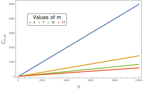
For large enough $n$, the topological complexity asymptotes to

However, a more careful analysis shows that this an approximate behavior, since the apparent straight lines in the plot actually exhibit an internal structure with a periodic pattern of fluctuations that becomes more noticeable as $m$ increases. The situation is illustrated in Figure 7 for $m=30$: the apparent single line is made of two discrete series of points that sit along two parallel lines. For other values of $m$ this pattern can be different. Even though we have no algebraic explanation for these patterns, we checked that they have the same asymptotic slope.

Interestingly, the topological complexity (32) can be given a nice geometric interpretation in terms of the Farey tesselation of the upper half-plane Kulkarni. This tesselation is a result of embedding the Farey graph $\mathcal{F}$ on the upper-half plane, whose vertices are the rational numbers (plus infinity) and whose edges join each pair of Farey neighbors (and only these). It is constructed as follows: one first draws vertical lines at each integer point $n=\frac{n}{1}\in\mathbb{Z}$, which reflects the fact that all integers are Farey neighbors of $\infty$; then joins pairs of adjacent points by a semicircle and generates a new rational point in between the two using the mediant formula $\tfrac{n_{1}}{m_{1}}\oplus\tfrac{n_{2}}{m_{2}}=\tfrac{n_{1}+n_{2}}{m_{1}+m_{2}}$. The procedure then follows recursively, and the result is shown by the black curves in Figure 8. The resulting tiles are ideal triangles with vertices either at a rational number or at infinity, and edges along semicircles of different radii or along the vertical lines.¹⁶¹⁶ 16 It can be proven that $i)$ two triangles are either equal or disjoint; $ii)$ every triangle is adjacent to exactly three other triangles; $iii)$ modular transformations map between different triangles, or, in other words, the Farey tesselation is invariant under $PSL(2,\mathbb{Z})$. One can also define the dual tree graph $\mathcal{F}^{*}$ of $\mathcal{F}$ by taking the baricenter of each ideal triangle as vertices and connecting them to the adjacent triangles, forming a trivalent tree.

References

- (1) S. Aaronson, The Complexity of Quantum States and Transformations: From Quantum Money to Black Holes, 2016. 1607.05256.
- (2) M. A. Nielsen, M. R. Dowling, M. Gu and A. C. Doherty, Quantum Computation as Geometry, Science 311 (Feb., 2006) 1133–1135, [quant-ph/0603161].
- (3) D. Stanford and L. Susskind, Complexity and Shock Wave Geometries, Phys. Rev. D90 (2014) 126007, [1406.2678].
- (4) A. R. Brown, D. A. Roberts, L. Susskind, B. Swingle and Y. Zhao, Holographic Complexity Equals Bulk Action?, Phys. Rev. Lett. 116 (2016) 191301, [1509.07876].
- (5) R. A. Jefferson and R. C. Myers, Circuit complexity in quantum field theory, JHEP 10 (2017) 107, [1707.08570].
- (6) S. Chapman, M. P. Heller, H. Marrochio and F. Pastawski, Toward a Definition of Complexity for Quantum Field Theory States, Phys. Rev. Lett. 120 (2018) 121602, [1707.08582].
- (7) M. Guo, J. Hernandez, R. C. Myers and S.-M. Ruan, Circuit Complexity for Coherent States, JHEP 10 (2018) 011, [1807.07677].
- (8) L. Hackl and R. C. Myers, Circuit complexity for free fermions, JHEP 07 (2018) 139, [1803.10638].
- (9) R. Khan, C. Krishnan and S. Sharma, Circuit Complexity in Fermionic Field Theory, Phys. Rev. D98 (2018) 126001, [1801.07620].
- (10) M. Sinamuli and R. B. Mann, Holographic Complexity and Charged Scalar Fields, 1902.01912.
- (11) A. Bhattacharyya, A. Shekar and A. Sinha, Circuit complexity in interacting QFTs and RG flows, JHEP 10 (2018) 140, [1808.03105].
- (12) D. W. F. Alves and G. Camilo, Evolution of complexity following a quantum quench in free field theory, JHEP 06 (2018) 029, [1804.00107].
- (13) H. A. Camargo, P. Caputa, D. Das, M. P. Heller and R. Jefferson, Complexity as a novel probe of quantum quenches: universal scalings and purifications, Phys. Rev. Lett. 122 (2019) 081601, [1807.07075].
- (14) T. Ali, A. Bhattacharyya, S. Shajidul Haque, E. H. Kim and N. Moynihan, Time Evolution of Complexity: A Critique of Three Methods, 1810.02734.
- (15) S. Liu, Complexity and scaling in quantum quench in dimensional fermionic field theories, 1902.02945.
- (16) R.-Q. Yang, Complexity for quantum field theory states and applications to thermofield double states, Phys. Rev. D97 (2018) 066004, [1709.00921].
- (17) R.-Q. Yang, C. Niu, C.-Y. Zhang and K.-Y. Kim, Comparison of holographic and field theoretic complexities for time dependent thermofield double states, JHEP 02 (2018) 082, [1710.00600].
- (18) S. Chapman, J. Eisert, L. Hackl, M. P. Heller, R. Jefferson, H. Marrochio et al., Complexity and entanglement for thermofield double states, 1810.05151.
- (19) J. Jiang and X. Liu, Circuit Complexity for Fermionic Thermofield Double states, Phys. Rev. D99 (2019) 026011, [1812.00193].
- (20) T. Ali, A. Bhattacharyya, S. Shajidul Haque, E. H. Kim and N. Moynihan, Post-Quench Evolution of Distance and Uncertainty in a Topological System: Complexity, Entanglement and Revivals, 1811.05985.
- (21) F. Liu, R. Lundgren, P. Titum, J. R. Garrison and A. V. Gorshkov, Circuit Complexity across a Topological Phase Transition, 1902.10720.
- (22) V. Balasubramanian, M. DeCross, A. Kar and O. Parrikar, Binding Complexity and Multiparty Entanglement, JHEP 02 (2019) 069, [1811.04085].
- (23) I. Akal, Weighting gates in circuit complexity and holography, 1903.06156.
- (24) R.-Q. Yang, Y.-S. An, C. Niu, C.-Y. Zhang and K.-Y. Kim, Principles and symmetries of complexity in quantum field theory, Eur. Phys. J. C79 (2019) 109, [1803.01797].
- (25) R.-Q. Yang, Y.-S. An, C. Niu, C.-Y. Zhang and K.-Y. Kim, More on complexity of operators in quantum field theory, JHEP 03 (2019) 161, [1809.06678].
- (26) R.-Q. Yang and K.-Y. Kim, Complexity of operators generated by quantum mechanical Hamiltonians, JHEP 03 (2019) 010, [1810.09405].
- (27) P. Caputa and J. M. Magan, Quantum Computation as Gravity, 1807.04422.
- (28) J. M. Magán, Black holes, complexity and quantum chaos, JHEP 09 (2018) 043, [1805.05839].
- (29) P. Caputa, N. Kundu, M. Miyaji, T. Takayanagi and K. Watanabe, Anti-de Sitter Space from Optimization of Path Integrals in Conformal Field Theories, Phys. Rev. Lett. 119 (2017) 071602, [1703.00456].
- (30) P. Caputa, N. Kundu, M. Miyaji, T. Takayanagi and K. Watanabe, Liouville Action as Path-Integral Complexity: From Continuous Tensor Networks to AdS/CFT, JHEP 11 (2017) 097, [1706.07056].
- (31) A. Bhattacharyya, P. Caputa, S. R. Das, N. Kundu, M. Miyaji and T. Takayanagi, Path-Integral Complexity for Perturbed CFTs, JHEP 07 (2018) 086, [1804.01999].
- (32) T. Takayanagi, Holographic Spacetimes as Quantum Circuits of Path-Integrations, 1808.09072.
- (33) E. Witten, Quantum Field Theory and the Jones Polynomial, Commun. Math. Phys. 121 (1989) 351–399.
- (34) M. Bos and V. P. Nair, U(1) Chern-Simons Theory and c=1 Conformal Blocks, Phys. Lett. B223 (1989) 61–66.
- (35) M. Bos and V. P. Nair, Coherent State Quantization of Chern-Simons Theory, Int. J. Mod. Phys. A5 (1990) 959.
- (36) J. M. F. Labastida, P. M. Llatas and A. V. Ramallo, Knot operators in Chern-Simons gauge theory, Nucl. Phys. B348 (1991) 651–692.
- (37) K. Murasugi, Knot Theory and Its Applications. Birkhäuser, Boston, US, 1st ed., 1996.
- (38) H. W. Lin, Cayley graphs and complexity geometry, JHEP 02 (2019) 063, [1808.06620].
- (39) A. F. Beardon, M. Hockman and I. Short, Geodesic continued fractions, Michigan Math. J. 61 (03, 2012) 133–150.
- (40) G. P. Collins, Computing with quantum knots, Scientific American 294 (2006) 56–63.
- (41) C. Nayak, S. H. Simon, A. Stern, M. Freedman and S. Das Sarma, Non-Abelian anyons and topological quantum computation, Reviews of Modern Physics 80 (Jul, 2008) 1083–1159, [0707.1889].
- (42) D. Melnikov, A. Mironov, S. Mironov, A. Morozov and A. Morozov, Towards topological quantum computer, Nucl. Phys. B926 (2018) 491–508, [1703.00431].
- (43) G. Kuperberg, How hard is it to approximate the Jones polynomial?, arXiv e-prints (Aug, 2009) arXiv:0908.0512, [0908.0512].
- (44) I. Cherednik, Jones polynomials of torus knots via DAHA, 1111.6195.
- (45) M. H. Freedman, A. Kitaev and Z. Wang, Simulation of topological field theories by quantum computers, Commun. Math. Phys. 227 (2002) 587–603, [quant-ph/0001071].
- (46) P. Freyd, D. Yetter, J. Hoste, W. B. R. Lickorish, K. Millett and A. Ocneanu, A new polynomial invariant of knots and links, Bull. Am. Math. Soc. 12 (1985) 239–246.
- (47) J. Przytycki and P. Traczyk, Conway Algebras and Skein Equivalence of Links, Proc. Amer. Math. Soc. 100 (1987) 744–748.
- (48) L. H. Kauffman, An invariant of regular isotopy, Trans. Amer. Math. Soc. 312 (1990) 417–471.
- (49) A. Hatcher, Algebraic Topology. Cambridge University Press, New York, NY, USA, 1st ed., 2001.
- (50) G. Salton, B. Swingle and M. Walter, Entanglement from Topology in Chern-Simons Theory, Phys. Rev. D95 (2017) 105007, [1611.01516].
- (51) V. Balasubramanian, J. R. Fliss, R. G. Leigh and O. Parrikar, Multi-Boundary Entanglement in Chern-Simons Theory and Link Invariants, JHEP 04 (2017) 061, [1611.05460].
- (52) S. Dwivedi, V. K. Singh, S. Dhara, P. Ramadevi, Y. Zhou and L. K. Joshi, Entanglement on linked boundaries in Chern-Simons theory with generic gauge groups, JHEP 02 (2018) 163, [1711.06474].
- (53) V. Balasubramanian, M. DeCross, J. Fliss, A. Kar, R. G. Leigh and O. Parrikar, Entanglement Entropy and the Colored Jones Polynomial, JHEP 05 (2018) 038, [1801.01131].
- (54) D. Melnikov, A. Mironov, S. Mironov, A. Morozov and A. Morozov, From Topological to Quantum Entanglement, 1809.04574.
- (55) E. Guadagnini, The Universal link polynomial, Int. J. Mod. Phys. A7 (1992) 877–946.
- (56) E. Guadagnini, M. Martellini and M. Mintchev, Wilson Lines in Chern-Simons Theory and Link Invariants, Nucl. Phys. B330 (1990) 575–607.
- (57) M. Marino and C. Vafa, Framed knots at large N, Contemp. Math. 310 (2002) 185–204, [hep-th/0108064].
- (58) R. K. Kaul, Topological quantum field theories: A Meeting ground for physicists and mathematicians, hep-th/9907119.
- (59) D. Gepner and E. Witten, String Theory on Group Manifolds, Nucl. Phys. B278 (1986) 493–549.
- (60) https://knotplot.com/.
- (61) P. Bantay, Mapping class group representations and Conformal Field Theory, arXiv Mathematics e-prints (Jan., 2005) , [math/0501443].
- (62) A. Coste and T. Gannon, Congruence subgroups and rational conformal field theory, math/9909080.
- (63) S.-H. Ng and P. Schauenburg, Congruence Subgroups and Generalized Frobenius-Schur Indicators, Commun. Math. Phys. 300 (2010) 1–46, [0806.2493].
- (64) J. CONWAY, An enumeration of knots and links, and some of their algebraic properties, in Computational Problems in Abstract Algebra (J. LEECH, ed.), pp. 329 – 358. Pergamon, 1970. DOI.
- (65) R. S. Kulkarni, An Arithmetic-Geometric Method in the Study of the Subgroups of the Modular Group, American Journal of Mathematics 113 (1991) 1053–1133.
- (66) S. Schleimer, Notes on the complex of curves, unpublished notes (2006) .
- (67) M. Alishahiha, Holographic complexity, Physical Review D 92 (2015) 126009.
- (68) R. Abt, J. Erdmenger, H. Hinrichsen, C. M. Melby-Thompson, R. Meyer, C. Northe et al., Topological Complexity in AdS3/CFT2, Fortsch. Phys. 66 (2018) 1800034, [1710.01327].
- (69) Y. I. Manin and M. Marcolli, Holography principle and arithmetic of algebraic curves, Adv. Theor. Math. Phys. 5 (2002) 617–650, [hep-th/0201036].
- (70) M. Freedman and V. Krushkal, On the asymptotics of quantum representations of mapping class groups, Forum Mathematicum 18 (2006) 293–304.
- (71) J. Marché and M. Narimannejad, Some asymptotics of topological quantum field theory via skein theory, Duke Mathematical Journal 141 (2008) 573–587.
- (72) J. r. E. Andersen, Asymptotic faithfulness of the quantum representations of the mapping class groups, Annals of Mathematics. Second Series 163 (2006) 347–368.
- (73) L. Charles and J. Marché, Knot state asymptotics I: AJ conjecture and Abelian representations, Publications Mathématiques. Institut de Hautes Études Scientifiques 121 (2015) 279–322.
- (74) L. Charles and J. Marché, Knot state asymptotics II: Witten conjecture and irreducible representations, Publications Mathématiques. Institut de Hautes Études Scientifiques 121 (2015) 323–361.
- (75) I. Dynnikov and B. Wiest, On the complexity of braids, Journal of the European Mathematical Society (2007) 801–840.
- (76) E. Verlinde, Fusion rules and modular transformations in 2d conformal field theory, Nuclear Physics B 300 (1988) 360 – 376.
- (77) S. Duzhin and M. Shkolnikov, A formula for the HOMFLY polynomial of rational links, Arnold Math. J. 1 (2015) 345–359, [1009.1800].
- (78) G. Camilo, S. Eliens, D. Melnikov, F. Novaes and A. Prudenziati, in preparation, .
- (79) H. Schubert, Knoten mit zwei brücken, Mathematische Zeitschrift 65 (Dec, 1956) 133–170.
- (80) A. M. Polyakov, Quantum Geometry of Bosonic Strings, Phys. Lett. B103 (1981) 207–210.
- (81) M. Miyaji and T. Takayanagi, Surface/State Correspondence as a Generalized Holography, PTEP 2015 (2015) 073B03, [1503.03542].
- (82) P. H. Ginsparg and G. W. Moore, Lectures on 2-D gravity and 2-D string theory, in Proceedings, Theoretical Advanced Study Institute (TASI 92): From Black Holes and Strings to Particles: Boulder, USA, June 1-26, 1992, pp. 277–469, 1993. hep-th/9304011.
- (83) D. Singerman and J. Strudwick, The Farey Maps Modulo N, 1803.08851.
- (84) J. M. F. Labastida and E. Perez, A Relation between the Kauffman and the HOMFLY polynomials for torus knots, J. Math. Phys. 37 (1996) 2013, [q-alg/9507031].