Beam Selection and Discrete Power Allocation in Opportunistic Cognitive Radio Systems with Limited Feedback Using ESPAR AntennasThanks: Parts of this research were presented at 53nd Annual Conference on Information Sciences and Systems (CISS), 2019 [1]. This research is supported by the NSF under grant ECCS-1443942.
Abstract
We consider an opportunistic cognitive radio (CR) system consisting of a primary user (PU), secondary transmitter (SU), and secondary receiver (SU), where SU is equipped with an electrically steerable parasitic array radiator (ESPAR) antenna with beam steering capability for sensing and communication, and there is a limited feedback channel from SU to SU. Taking a holistic approach, we develop a framework for integrated sector-based spectrum sensing and sector-based data communication. Upon sensing the channel busy, SU determines the beam corresponding to PU’s orientation. Upon sensing the channel idle, SU transmits data to SU, using the selected beam corresponding to the strongest channel between SU and SU. We formulate a constrained optimization problem, where SU-SU link ergodic capacity is maximized, subject to average transmit power and interference constraints, and the optimization variables are sensing duration, thresholds of channel quantizer at SU, and transmit power levels at SU. Since this problem is non-convex we develop a suboptimal computationally efficient iterative algorithm to find the solution. Our numerical results quantify the capacity improvement provided by the ESPAR antenna and demonstrate that our CR system yields lower outage and symbol error probabilities, compared with a CR system that its SU has an omni-directional antenna.
Index Terms:
Beam selection, cognitive radio, constrained ergodic capacity maximization, discrete power allocation, ESPAR antenna, imperfect channel sensing, error-free bandwidth limited feedback channel, reconfigurable antennas.I Introduction
I-A Overview and Background
Cognitive radio (CR) is a promising solution that enhances spectrum utilization by allowing an unlicensed or secondary user (SU) to access licensed bands in a such way that its imposed interference on license holder primary users (PUs) is limited, and hence fills the spectrum holes in time and/or frequency domains [2, 3, 4, 5, 6, 7]. There is a rich literature on underlay CR systems, where PUs and SUs are allowed to transmit simultaneously and in the same frequency band, as long as the interference caused by SUs to PUs stays below a pre-determined threshold. While underlay systems do not require spectrum sensing to detect PU’s activities, they demand coordination between PUs and SUs (to obtain channel state information (CSI) of PU links at SUs) that is not always feasible. On the other hand, interweave or opportunistic CR systems utilize spectrum sensing to enable SUs to use a licensed frequency band during a time interval, only if PUs are not using that frequency band within that time interval, implying that coordination between PUs and SUs to acquire CSI is not needed.
Reconfigurable antennas (RA) [8, 9], with the capabilities of dynamically modifying their characteristics (e.g., operating frequency, beamwidth, radiation pattern, polarization) can improve the spectral efficiency (well beyond what is attainable with omni-directional antennas), via beam steering and utilizing the spectrum white spaces in spatial (angular) domain. RAs have been used to design directional wireless and millimeter-wave communication systems and surveillance [10]. An electrically steerable parasitic array radiator (ESPAR) antenna is a special kind of RAs, that has been used for identifying the spectral holes in spatial domain in CR systems. ESPAR divides the angular domain into several sectors (beams) and switches between beampatterns of sectors in a time-division fashion (only one of beams is active at a time). The ESPAR antenna relies on a single RF front end (an active element) coupled to several passive or parasitic elements (mutually coupled to the active one) to steer beams in prescribed directions [11, 12]. The active element is connected to the transmitter/receiver circuit and the parasitic elements are reactively loaded. Since only one RF chain is needed, the power consumption, cost, and hardware complexity are significantly reduced. The mutual coupling between the ESPAR antenna elements is created by reducing the spacing between them, which makes this antenna suitable for small mobile devices. For CR systems, the ESPAR antennas provide an improved spectrum sensing, due to a signal-to-noise ratio (SNR) increase for transmission and reception of directional signals, and limit out-of-band interference to and from PUs [13]. The ESPAR antennas have the capability of transmitting multiple data streams by signal projection on beamspace basis [14]. Also, they can be used for blind interference alignment through beampattern switching [15]. ESPAR antennas have been used in [16], to provide an end-to-end solution for practically implementable cloud radio access networks. RAs can enhance performance of multiple-input multiple-output (MIMO) systems, via enabling joint beam and antenna selection optimization [17, 18, 19].
Motivated by the benefits of ESPAR antennas, in this work we consider an opportunistic CR system, where SU transmitter (SU) is equipped with an ESPAR antenna, and SU uses the directions (identified during spectrum sensing phase), for data communication with SU receiver (SU) with an optimized discrete power level. To the best of our knowledge, this is the first work that proposes a holistic system design for integrated sector-based spectrum sensing and sector-based data communication for opportunistic CR systems using ESPAR.
I-B Spectrum Sensing in Opportunistic CR Systems Using ESPAR Antennas
Considering the ESPAR antennas, the authors in [13, 20, 21, 22] designed detectors, based on the received signal energy in different beams, and also eigenvalue-based detectors, via constructing the covariance matrix that captures the signal correlation across beams. The advantages of spectrum sensing using ESPAR antennas are twofold. First, the SNR gain from the directional beampatterns increases the probability of detecting PU’s activities within that beam, and hence decreases the chance of causing interference on PU. Second, the discovered unoccupied beams in spatial (angular) domain during spectrum sensing represents directional transmit/receive opportunities for SUs, which can be utilized to increase spectral efficiency (opportunities that would be missed when using an omni-directional antenna at SU).
I-C Beam Selection for Data Communication in Underlay CR Systems Using RA Antennas
Selecting the best beam for data communication has been considered before in [23, 24, 25, 26] using general/traditional directional antennas (with multi-RF chain) and in [17, 18, 19, 27, 28] using RAs for underlay CR systems. For instance, the authors in [17] considered space-shift keying (SSK) signaling and investigated the best beam selection method that improves SSK performance (in terms of throughput, system complexity, error probability), via minimizing the Rician -factor and the correlation coefficient between the antenna beams. Considering SSK signaling, the authors in [18] proposed a beam selection scheme that improves the performance of the secondary system, while meeting the transmit power and outage interference constraints (without any feedback from the receiver). For a multiuser orthogonal frequency-division multiple access (OFDMA) underlay CR network, the authors in [28] developed a game theoretical framework for joint optimization of beam and subcarrier selection at each SU, such that the overall network capacity is maximized, while the interference constraint on the primary network is met. The authors in [19] studied a different scenario where SU is equipped with multiple RAs and beam selection is conducted based on the channel between SU and SU and considering several performance metrics (achievable rate, error and outage probabilities). The work in [27] shows that comparing RA and traditional antenna selection, the former can offer significant improvements in SNR.
I-D Beamforming for Data Communication Using ESPAR Antennas
A related research thrust in the context of ESPAR antennas for CR systems is designing adaptive beampatterns (also called beamforming) [13, 29, 30, 31, 32]. For instance, the authors in [13] proposed an adaptive beamforming algorithm, that numerically optimizes the beampattern and antenna efficiency, and creates beampattern nulls to protect PU from unwarranted transmissions by SUs. However, such a design approach from a mathematical perspective is very challenging, due to the tunable reactive loads, which renders the problem a non-convex optimization without any closed form solution. Furthermore, implementing the design incurs high computational complexity. [29] utilized the switchable weakly-correlated patterns of an ESPAR antenna for underlay CR systems, in order to maximize the transmitted power to SU while limiting interference imposed on PU. [30] presented several numerical methods for SNR optimization and beam-null steering via maximizing the cross-correlation coefficient between a known reference (pilot) and the received signals. [31] proposed a minimum variance distortionless response (MVDR) beamforming method which steers the beam at the desired direction and places nulls at the interfering directions. [32] designed a robust precoding scheme for a MIMO CR system, where the CR interference channel is completely unknown. We note that the implicit assumption in these works is that the directions of PU and SU with respect to SU are known and hence the shape of the beam can be optimized accordingly. Thus, the beamforming designs in [13, 29, 30, 31, 32] are not directly applicable to a problem where these direction information are missing.
I-E Knowledge Gap and Our Motivation
Our review of the literature indicates that the studies on optimizing spectrum sensing and optimizing data communication have been pursued as two separate research thrusts: the works cited in Section I-B focus on spectrum sensing in opportunistic CR systems, whereas the works in Section I-C and Section I-D focus on data communication in underlay CR systems. The developed beam selection and beamforming schemes in these works are specifically tailored for underlay CR systems, which do not require spectrum sensing to detect PU’s activities, and rely on the knowledge obtained from coordination between PUs and SUs. Evidently, the literature lacks a holistic system design, that integrates spectrum sensing and data communication in a cohesive manner for opportunistic CR systems. Such a holistic system design needs to take into consideration the effect of imperfect spectrum sensing on data communication optimization. This is the motivation behind our work. Taking full advantage of beam steering capability of the ESPAR antenna (the capability of choosing one beam among beams), we propose an integrated design for an opportunistic CR system, where SU is equipped with an ESPAR antenna. We leverage on the beam steering capability of the ESPAR antenna for both spectrum sensing and data communication optimization. Different from the state-of-the-art, our proposed integrated design incorporates induced errors due to: (i) imperfect spectrum sensing and determining the correct beam corresponding to PU’s location, such errors affect the interference imposed on PU; (ii) selecting the best beam for data communication over SU-SU link.
I-F Our Contributions and Paper Organization
In this paper, we consider an opportunistic CR system consisting of a PU, SU, and SU, where SU is equipped with an ESPAR antenna with the capability of choosing one sector among sectors for its data transmission to SU. During the initial channel sensing phase SU senses the channel and monitors the activity of PU. While being in this phase, SU determines the beam corresponding to the location (orientation) of PU based on the received signal energy. SU stays in this phase as long as the channel is sensed busy. It leaves this phase and enters transmission phase when the channel is sensed idle. The transmission phase itself consists of two phases: channel training phase followed by data transmission phase. During the former phase, SU sends pilot symbols to enable channel training and estimation at SU as well as selection of the strongest channel among all beams between SU-SU for data transmission. Also, SU employs an -bit quantizer to quantize the gain of the selected beam. Then, SU feeds back the index of the selected beam as well as the -bit representation of the index of the quantization interval over an error-free bandwidth limited feedback link to SU, so SU can optimally adapt its discrete power level accordingly. The main contributions of this paper can be summarized as follows:
- •
Given this system model, we formulate a novel optimization problem, aiming at maximizing the constrained ergodic capacity of SU-SU link, subject to average interference and average transmit power constraints.
- •
Our problem formulation takes into consideration the effect of imperfect spectrum sensing as well as the error due to incorrect determination of the beam corresponding to PU’s location (and its corresponding effect on imposed average interference) occurred during channel sensing and monitoring phase.
- •
Our problem formulation also takes into account the probability of correct determination of the strongest beam for data transmission from SU to SU, occurred during channel training phase. It also incorporates the impact of CSI quantization on the constrained optimization problem in hand.
- •
We solve the formulated problem and optimize the duration of spectrum sensing, thresholds of CSI quantizer, and discrete transmit power levels (to be employed at SU) corresponding to CSI quantization intervals.
- •
For our system model, we provide closed form expressions for outage and symbol error probabilities.
- •
To the best of our knowledge, this is the first work that adopts a holistic approach to design an opportunistic CR system using ESPAR antennas and integrates sector-based spectrum sensing and sector-based data communication. All cited works use RAs for enhanced communication in underlay CR systems. Utilizing ESPAR antennas for opportunistic spectrum sharing systems is a highly promising solution to enhance the performance of secondary links, while satisfying the constraints set by the primary links [28].
- •
This work is different from our preliminary works in [33, 34, 35], where we have considered a simpler constrained optimization problem (with different optimization variables, including continuous transmit power and direction of antenna steering of SU), assuming that SU knows the direction (angle) corresponding to PU’s activities. It is also different from our work in [1], where we have assumed that SU knows the location of SU and PU, and, perfect CSI of SU-SU link is available and used for transmit power adaptation. This work is different from [36], in which the direction of PU is estimated at SU (i.e., it is not based on determining the sector).
- •
Taking advantage of the additional degrees of freedom offered by ESPAR antennas with variable beam directions, we improve the spectral efficiency and reduce implementation complexity of opportunistic spectrum sharing systems, while fulfilling an average interference constraint imposed on PU. Our simulations demonstrate and quantify the capacity improvement provided by the ESPAR antenna, in terms of average transmit power and average interference constraints. For instance, at dB, dB, the capacity of our CR system is times larger than the capacity of a CR system that its SU has an omni-directional antenna.
- •
Our numerical results show that with only a small number of feedback bits the capacity of our opportunistic CR system approaches to its baseline, which assumes the full knowledge of unquantized SU-SU channel gain at SU.
The remainder of the paper is organized as follows. Section II explains our system model and problem statement. Section III characterizes the objective function and the constraints of our optimization problem, in terms of the optimization variables. Specially, in Section III-A we describe our binary energy-based detector for detecting PU activity and in Section III-B we express how SU determines the beam corresponding to PU. In Section III-C we discuss how SU determines the strongest channel between SU-SU and we obtain the probability of selecting the true strongest channel among all beams. The problem is formalized and solved in Section IV and the closed form expressions for outage and symbol error probabilities are given in Section V. Section VI presents our simulation results and Section VII concludes the paper.
II System Model and Problem Statement
II-A Background on ESPAR Antennas
The ESPAR antenna is a circular array, comprised of one active element and parasitic elements symmetrically surrounding the active element, and the radius of the array is , where is the carrier wavelength [11]. Fig. 1(a) depicts an ESPAR structure. The active element is connected to the single RF chain, while parasitic elements (which are mutually coupled to the active element) are short-circuited and loaded by variable reactive loads. Let be the reactive load of -th element and vector denote the reactive loads of all parasitic elements. By adjusting these reactive loads, the beampatterns of the ESPAR antenna are designed such that the angular space is divided into spatial sectors or beams11 1 Throughout this paper, “sector” and “beam” are used interchangeably.. In particular, to design the beampattern corresponding to the first beam, entries of vector are optimized such that the beam gain is maximized at an angle (for example angle ) [11]. Since the ESPAR antenna structure is symmetric, the beampattern corresponding to the second beam can be obtained by circularly shifting the entries of , such that the beam gain is maximized at angle . Repeating this times one can obtain beampatterns corresponding to beams such that the beampattern corresponding to the -th beam achieves its maximum at angle for . It is noteworthy that the ESPAR antenna can provide an omni-directional beampattern if the reactive loads of all parasitic elements are chosen equal (omni-directional mode).

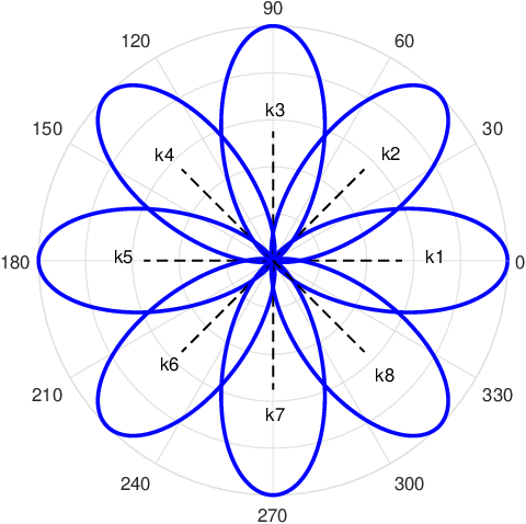
Similar to [36], to mathematically model the radiation pattern (antenna pattern) of the ESPAR antenna, we adopt the Gaussian pattern in azimuth plane in terms of angle given by
| (1) |
| (2) |
denotes the remainder of , constant , is the 3-dB beamwidth, and are two constant antenna parameters. The radiation pattern of -th sector at angle is
| (3) |
In Fig. 1(b), the beampatterns of an ESPAR antenna with parasitic elements are shown. In this paper, we discuss the received or transmitted signal at -th sector of SU. This means that, during the signal reception or transmission, the reactive loads of all parasitic elements (i.e., the entries of vector ) are set and tuned such that the beampattern corresponding to the -th beam is generated. Note that in our work we assume the reactive loads (i.e., the entries of vector and thus the shapes of beampatterns or equivalently the radiation patterns of sectors) are determined by the ESPAR antenna designer. Given the antenna design, we focus on how the sector-based structure of this ESPAR antenna can be exploited to enhance the system performance of our opportunistic CR system, in which SU optimizes its sector-based data communication to SU according to the results of its sector-based channel sensing.
II-B Geometry of Our Opportunistic CR System
Our CR system model is illustrated in Fig. 2, consisting of a PU and a pair of SU and SU. We note that PU in our system model can be a primary transmitter or receiver. We assume when PU is active it is engaged in a bidirectional communication with another PU, which is located far from SU and hence its activity does not impact our analysis. We assume SU is equipped with an ()-element ESPAR antenna (for channel sensing and communication) with the capability of choosing one sector among sectors for its data transmission to SU, while SU and PU use omni-directional antennas. The reason for this assumption is to focus on quantifying the capacity improvement provided by the ESPAR antenna at SU, in the presence of channel sensing error as well as average transmit power constraint and average interference constraint. We also assume there is an error-free bandwidth limited feedback channel from SU to SU (where the channel bandwidth is measured in terms of the number of bits sent over the channel [37, 38], to help SU select the best sector for its data transmission to SU and also to provide SU with the quantized channel gain of the selected beam, so SU can adapt its discrete power level accordingly. The direction (orientation) of PU and SU with respect to SU are denoted by angles , and , receptively. Clearly, in our problem SU does not know these directions or angles (otherwise, the beam selection at SU for data transmission would become trivial).
Let , , denote the fading coefficients of channels between SU and PU, SU and SU, and SU and PU, respectively, when the ESPAR antenna of SU is in omni-directional mode. We model these fading coefficients as independent circularly symmetric complex Gaussian random variables. We assume , and are independent exponentially distributed random variables with mean , and , respectively22 2 We note that the distances between users are included in the small scale fading model [39]. In particular, we assume that the mean values are , where is the reference distance, is the path-loss exponent, and and are the distances between SU and PU, SU and SU, and SU and PU, respectively. Since in our problem SUs and PU cannot cooperate, SUs cannot estimate and . However, we assume that SU knows the channel statistics, i.e., the mean values and . Let and denote the fading coefficients of channel between -th sector of SU and PU, and between -th sector of SU and SU, respectively, when the ESPAR antenna of SU is in directional mode, where , . We assume the channel gain is an exponential random variable with mean , and SU knows , for all [28]. For the readers’ convenience, we have collected the most commonly used symbols in Table I.

| Symbol | Description |
|---|---|
| Number of beams | |
| Number of samples used for sensing and monitoring | |
| Number of bits for quantization at SU | |
| Radiation pattern of -th beam at angle | |
| Fading coefficient of channel between -th beam of | |
| SU and PU | |
| Fading coefficient of channel between -th beam of | |
| SU and SU | |
| Mean of channel gain between -th beam of | |
| SU and SU | |
| Channel gain of selected beam for data transmission | |
| from SU to SU | |
| Directions of PU and SU with respect to SU | |
| Indices of selected beam for PU and SU | |
| Prior probabilities of and | |
| Probabilities of channel being sensed idle or busy | |
| Duration of frame employed by SU | |
| Duration of channel sensing and monitoring phase |
II-C Our Problem Statement
Suppose, SUs employ a frame with a fixed duration of seconds, depicted in Fig. 3. We assume SU first senses the channel and monitors the activity of PU. We refer to this period as channel sensing and monitoring phase (with a variable duration of seconds). Depending on the outcome of this phase, SU stays in this phase or enters the next phase, which we refer to as transmission phase. The transmission phase itself consists of two phases: channel training phase (with a fixed duration of seconds) followed by data transmission phase (with a variable duration of seconds). During the former phase, SU sends pilot symbols to enable channel training and estimation at SU. During the latter phase, SU sends data symbols to SU. Given and we have . In the following, we describe how SU operates in directional mode during these three distinct phases. Based on these descriptions, we provide our problem statement.
Channel Sensing and Monitoring Phase: During this phase SU senses the channel and monitors the activity of PU. Suppose and represent the binary hypotheses of PU being active and inactive, respectively, with prior probabilities and . SU applies a binary detection rule, as will be described in Section III-A, to decide whether or not PU is active. Let and denote the detector outcome, i.e., the detector finds PU active (channel is sensed busy and occupied) and inactive (channel is sensed idle and unoccupied and thus can be used by SU for transmission), respectively. The accuracy of this binary detector is characterized by its false alarm probability and detection probability . Therefore, the probabilities of events and become and , respectively. Furthermore, the joint probabilities are and . The accuracy of channel sensing impacts the maximum information rate that SU can transmit reliably to SU. Our problem formulation incorporates the effect of imperfect channel sensing on the constrained ergodic capacity maximization. As long as the channel is sensed busy, SU stays in channel sensing and monitoring phase. While being in this phase, SU determines the beam corresponding to the location (orientation) of PU based on the received signal energy. We denote the sector index corresponding to PU’s location by . SU uses for adapting its discrete power level during data transmission phase. We note that, there is a non-zero error probability when SU determines the beam index , i.e., it is possible that is not the true beam index corresponding to PU. Our problem formulation takes into account the impact of this error probability on the constrained ergodic capacity maximization.
Channel Training Phase: When the channel is sensed idle, SU leaves channel sensing and monitoring phase and enters this new phase and sends pilot symbols over all beams. Based on the received training signal, SU estimates the channel gain for all beams and determines the strongest channel among all beams, and the corresponding beam index . Also, SU employs an -bit quantizer to quantize . The quantizer has thresholds, denoted by , satisfying , and has quantization intervals for . The quantization mapping rule follows: if the quantizer input lies in the interval then the quantizer output is , for . The index of quantization interval can be represented by -bits. Then, SU feeds back as well as the -bit representation of the index of the quantization interval to which belongs, over an error-free bandwidth limited feedback link to SU, so SU can optimally adapt its discrete power level accordingly. We take into account the probability of determining the true beam corresponding to SU as well as the probability of selecting the true strongest channel among all beams between SU and SU, on the constrained capacity maximization.
Data Transmission Phase: After channel training phase, SU enters data transmission phase and transmits data to SU over the selected beam . During this phase, SU adapts its discrete power level , where , using and the information received from SU through the feedback channel, such that the ergodic capacity of SU-SU link is maximized, subject to average interference and transmit power constraints. We let to indicate that when then SU does not transmit data to SU, since the channel is too weak.
Table II enumerates the sequential steps we take within each of the three phases: channel sensing and monitoring phase, channel training phase, and data transmission phase.
| Phase | Sequential steps in each phase |
|---|---|
| 1. Channel Sensing and Monitoring Phase | 1.1. SU senses the channel and monitors the activity of PU. |
| 1.2. As long as the channel is sensed busy, SU stays in this phase. | |
| 1.3. While being in this phase, SU determines the beam corresponding to the orientation of PU | |
| denoted by (based on the received signal energy). | |
| 1.4. When the channel is sensed idle, SU leaves this phase and enters the next phase. | |
| 2. Channel Training Phase | 2.1. SU sends pilot symbols over all beams. |
| 2.2. SU estimates the channel gain for all beams and determines the strongest channel among | |
| all beams and the corresponding beam index . | |
| 2.3. SU employs an -bit quantizer to quantize . | |
| 2.4. SU feeds back as well as the -bit representation of the index of the quantization interval | |
| to which belongs, over a feedback link to SU. | |
| 2.5 SU leaves this phase and enters the next phase. | |
| 3. Data Transmission Phase | 3.1. SU adapts its discrete power level , using and the information received from SU |
| through the feedback channel, such that the constrained ergodic capacity is maximized. | |
| 3.2. SU transmits data to SU with power over the selected beam . |
Remark: It is worth emphasizing that in our problem, SU does not know the angles and , defined in Section II-B (otherwise, the beam selection at SU for data transmission would become trivial). We take full advantage of beam steering capability of the ESPAR antenna that enables sector-based spectrum sensing and communication at SU. In this work, SU does not estimate the angles and . Instead it determines the indices of the sectors corresponding to PU and SU (i.e., SU finds and learns during channel sensing and monitoring phase and channel training phase, respectively). For mathematical tractability, we assume that these sectors are unchanged during a frame duration. Comparing with a CR system design that is based on angle (or directional of arrival) estimation at SU, using the sector-based sensing and communication improves the system design resilience against the mobility of users (as long as the determined sectors do not change due to mobility).
When spectrum sensing is imperfect, the capacity of SU-SU link can be written as [1]
| (4) |
where is the instantaneous capacity of this link corresponding to the event and , and is the statistical expectation operator. Let indicate the maximum allowed interference power imposed on PU and denote the maximum allowed average transmit power of SU. Given our aforementioned system model description and to enable mathematically expressing the average interference and transmit power constraints in our problem, we let indicate SU transmit power in terms of the channel gain of the selected beam between SU and SU. To satisfy the average interference constraint ,we have
| (5) |
and to satisfy the average transmit power constraint, we have
| (6) |
Notice that, had channel sensing have been ideal, and data communication between SU and SU would cause no interference on PU. The more accurate channel sensing is, the smaller is the power of interference signal imposed on PU. On the other hand, increasing the accuracy of channel sensing requires a longer and a shorter , given the frame duration . Reducing decreases the capacity in (4). Therefore, there is a tradeoff between increasing and decreasing the power of interference signal imposed on PU. Let be the cumulative distribution function (CDF) of (will be derived in Section III-C). Given the discrete power levels ’s and the quantization thresholds ’s, can be written as
| (7) |
Therefore, the constraints in (5) and (6) can be rewritten as
| (8) |
| (9) |
Our main objective is to find the optimal channel sensing and monitoring duration , the optimal quantization thresholds ’s for the channel gain quantizer employed at SU, and the optimal discrete power levels ’s corresponding to each quantization interval , such that the ergodic capacity in (4) is maximized, subject to average interference and transmit power constraints given in (8) and (9), respectively. In other words, we are interested in solving the following constrained optimization problem
III Characterizing Objective Function and Constraints in (II-C)
Characterizing the objective function and the constraints in (II-C) requires addressing the following three components. First, the performance of the binary detector employed by SU to detect PU activity during channel sensing and monitoring phase plays role in the objective function and the average interference constraint in (8) via , and in the average transmit power constraint in (9) via . Obviously, this performance depends on the choice of the detector. Section III-A describes our proposed binary detector, which is based on the energy of the collected measurements from all sectors of the ESPAR antenna at SU during this phase, and provides closed form expressions for and of this detector. Second, the error probability of finding the sector index corresponding to PU at SU during channel sensing and monitoring phase affects the average interference constraint in (8). This error probability depends on the mechanism through which SU determines this sector index. Section III-B explains how SU finds this beam index, using the received signal energy from all sectors of the ESPAR antenna during this phase, and derives closed form expression of the corresponding error probability. Third, the probability of finding the sector index corresponding to SU during channel training phase impacts the average interference constraint in (8). During data transmission phase SU sends data to SU over the selected beam . Section III-C discusses the method utilized by SU to find this beam index, using the received training signal transmitted by all sectors of SU antenna, and derives a closed form expression for the corresponding probability.
III-A Energy-Based Binary Detector for Channel Sensing Using ESPAR Antenna
Channel sensing at SU (detecting the activity of PU) during channel sensing and monitoring phase can be formulated as a binary hypothesis testing problem. Suppose when PU is active (present), it transmits signal with power . Let denote the discrete-time representation of received signal at -th sector of SU at time instant where is the sampling period. Assuming SU collects samples corresponding to each sector we can write
| (10) | ||||
We model the transmitted signal by PU as a zero-mean complex Gaussian random variable with variance and we assume SU knows . The term is the additive noise at -th sector of SU antenna and is modeled as . We assume that , and are mutually independent random variables. Since SU takes samples of the received signal for different sectors sequentially (in different time instants), and noise samples are independent and thus uncorrelated both in time and space (sector) domains. Under hypothesis , given , we have where . Under hypothesis , we have . The hypothesis testing problem at discrete time instant for -th sector is then given by
| (11) |
Our proposed energy-based binary detector uses all the collected samples from sectors (total of collected samples). Let be the energy of received signal at sector . We have
| (12) |
Under hypothesis and also under (given ), the sector energy is distributed as a central chi-square random variable with degrees of freedom. We consider the summation of energies of received signals over all sectors as the decision statistics given below
| (13) |
where is the decision threshold. We can rewrite as
| (14) |
Note that is the summation of random variables. When is large enough can be approximated as a Gaussian random variable. Thus, Under hypothesis , for large we invoke the central limit theorem (CLT), to approximate as Gaussian with distribution , where . Similarly, under hypothesis for large , can be approximated with another Gaussian with distribution where , and is given below
| (15) |
where
| (16a) | ||||
| (16b) | ||||
and . Then, the false alarm and detection probabilities of this detector are given as the following
| (17) |
where is the Q-function. For a given value of , the false alarm probability can be written as
| (18) |
III-B Determining the Beam Corresponding to PU
During channel sensing and monitoring phase when the channel is sensed busy, SU determines the beam corresponding to the orientation of PU based on the received signal energy . Ordering these calculated energies, SU selects the beam index corresponding to the largest energy among all sectors. For example, in Fig. 4(a), we have , that is, the third beam has received the largest amount of energy.


As we mentioned, under hypothesis , given (or equivalently given and ), the sector energy is distributed as a central chi-square random variable with degrees of freedom and its conditional pdf and CDF expressions are
| (19a) | |||
| (19b) | |||
where and is the lower incomplete gamma function
| (20) |
Let represent the average error probability of finding the sector index corresponding to PU, i.e., the probability that while the true orientation of PU belongs to the angular domain of -th sector, , for . To find we start with finding , which is the probability that the index of selected sector, given and , is . We have
| (21) |
in which and are the conditional pdf and CDF of given in (19). Without loss of generality, suppose . After some mathematical manipulations and taking expectation with respect to , in (III-B) can be written as
| (22) |
where
To illustrate the behavior of (averaged over fading gain ) we define and plot versus for and dB. Fig. 5(a) shows versus for and . We observe that when decreases from to , beam selection becomes more accurate, i.e., increases for , however, it decreases outside this angular interval. Fig. 5(b) plots versus for and . We observe that as increases beam selection becomes more accurate. For large , we can see that approaches one for and it is approximately zero outside this angular interval. Now, we are ready to find using . We have


| (23) |
Due to the symmetrical structure of the ESPAR antenna we have . Note that is the probability of selecting the correct beam and for is the probability of selecting the incorrect beam, leading to error probability in beam selection. The average error probability versus the index beam is shown in Figs. 6(a) and 6(b) for dB. As expected, increases and decreases as increases.


III-C Determining the Beam Corresponding to SU
When the channel is sensed idle, SU leaves channel sensing and monitoring phase and enters channel training phase. During this phase, SU sends pilot symbols over all beams to enable channel training and estimation at SU. Using the received training signal, SU estimates the channel gains corresponding to all sectors and determines the strongest channel among all beams and the corresponding beam index . For example, in Fig. 4(b), we have , i.e., the second beam has the largest channel gain. SU employs an -bit quantizer, with quantization thresholds and quantization intervals , to quantize and to find the quantization interval to which belongs to. Then, SU feeds back as well as the -bit representation of the index of the quantization interval to which belongs, over the feedback link to SU. Let denote the probability that . To characterize we need to find the CDF and pdf of , denoted as and , respectively. Note that given our assumptions, ’s are independent across sectors, however, not necessarily identically distributed. Therefore, can be written as
| (24) |
where . After simplification, (24) can be written as
| (25) |
where
From the CDF in (25), we can find the pdf
| (26) |
Similar to section III-B, we can express as the following
| (27) |
Without loss of generality, suppose . After some mathematical simplification, can be expressed as
| (28) |
where
IV Formalizing and Solving (II-C)
After channel training phase, SU enters data transmission phase. Going through the previous two phases, at this point SU knows the beam indices , as well as the index of quantization interval to which the largest channel gain belongs to. Knowing the quantization interval index, SU infers the quantized value of and adopts its discrete power level accordingly. For instance, if then the quantized is and the associated discrete power level is . From a system-level design perspective, one can optimize the quantization thresholds ’s and the associated discrete power levels ’s, such that the constrained capacity is maximized. Furthermore, the capacity expression itself and the power of interference signal imposed on PU during this phase depend on the accuracy of the energy-based binary detector in Section III-A, in a way that increasing the detector accuracy has a positive effect on lowering the interference power and a negative impact on enhancing the capacity itself. This implies that an optimal can exist that maximizes the constrained capacity. In the following we express and in terms of the optimization variables and we find the term in (8) using the analysis we have conducted in sections III-B and III-C. We modify the objective function and the constrains in terms of the optimization variables in Section IV-A. Then, we provide our solution to the problem in Section IV-B.
IV-A Formalizing (II-C) with Modified Objective Function and Constraints
Starting with the continuous valued and its corresponding continuous valued transmit power , we can write the expressions for the instantaneous capacity and in (4) as [33]
| (29) |
Since SUs and PU cannot cooperate, SU cannot estimate the channel gain and thus cannot be directly maximized at SU. Instead, we consider a lower bound on its average over , denoted as . Using the Jensen’s inequality [40], the lower bound on becomes
| (30) |
where . Let where is the lower bound on in (4). From now on, we focus on . Let and denote the discrete transmission rates when the quantization interval index of is , i.e., , quantized is , and discrete power level is . From (29) we have
| (31) |
Recall that the probability of quantized being in the interval is equal to . By averaging over all possible quantization intervals, we can rewrite in terms of the discrete transmission rates as the following:
| (32) |
Next, we focus on the constraint in (8) and find the term . Using the average probabilities derived in (23) and (27) we have
| (33) |
Then, the constraint in (8) can be written as
| (34) |
where is
| (35) |
We end this section with the statement of the constrained optimization problem we solve. In Section IV-B we solve the following constrained optimization problem
| (P2) | ||||
It is worth mentioning that (P2) includes the special case where the locations (orientations) of PU and SU are such that they belong to the same beam, with respect to SU. First, suppose . In this case, the interference imposed on PU increases and SU uses a small transmit power level , such that the average interference constraint in (34) is satisfied. Next, suppose . In this case SU uses a larger , compared with the case where (because SU wrongly assumes that PU and SU lie in two different beams/sectors). Although the instantaneous interference in this case becomes larger (compared with the case where ), the average interference constraint in (34) is still satisfied.
IV-B Solving (P2)
We note that (P2) is a non-convex problem and can be solved using exhaustive search, which can be computationally expensive. Therefore we develop an iterative suboptimal algorithm with a much less computational complexity, to find the local optimal solution using the Lagrangian method. The Lagrangian is
| (36) |
where and are the nonnegative Lagrange multipliers, associated with the average transmit power and interference constraints, respectively. The Lagrangian multipliers can be obtained using the subgradient method. Our iterative algorithm is based on the block coordinate descent algorithm (BCDA) which relies on the following principle: all variables expect one are assumed to be fixed and the optimal variable that minimizes (IV-B) is found. This process is iterated for all the variables until the final solution is reached. Convergence is achieved if there exists a single solution that minimizes (IV-B) at each iteration [37]. To apply the principle of BCDA algorithm in our problem, we consider the following. Assuming fixed ’s and , the problem (P2) becomes convex with respect to . Therefore, the optimal ’s that minimize (IV-B) are the solutions to the Karush-Kuhn-Tucker (KKT) optimality necessary and sufficient conditions
| (37) |
where . On the other hand, assuming fixed ’s and , the optimal ’s that minimize (IV-B) are the solutions to for , which is the first derivative of with respect to . Setting we reach (38). Note the values of and in (IV-B) and (38) are obtained by applying the constraints given in (34) and (9). Recall that and and hence and .
We are now ready to state our iterative algorithm to find the local optimal solution of (P2). In the first step, let be a value in the interval . We initiate and find using (IV-B). Having and we obtain using (38). We repeat this and iterate between (IV-B) and (38) until we find . At this point, we check whether or not . If is less (greater) than one, we increase (decrease) the initial value of and find a new set of values for and check for the condition . We continue changing the initial value of and finding new values for and checking for the condition , until we find the set of values such that this condition is satisfied. In the second step, given values reached at the end of the first step, we find that minimizes (IV-B), using search methods such as bisection method33 3 The problem in (P2) can be solved offline, based on the statistical information of the channels between SU-PU and SU-SU, the number of sectors , and the number of feedback bits . In particular, given each pair , there is a set of optimal solution for , . These sets of solutions are available a priori at SU. Also, the sets of are available a priori at SU. During channel training phase, SU can also send its finding to SU. With the knowledge of and , SU would know which set of quantization thresholds to use for quantizing . The idea of offline power allocation optimization with a limited feedback channel has been used before for distributed detection systems in wireless sensor networks [38].. A summary of our proposed iterative algorithm for solving (P2) is given in Algorithm 1.
| (38) |
2: Set .
3: repeat
4: repeat
5: Find using (IV-B).
6: for
7: Having , obtain using (38).
8: Having , obtain using (IV-B).
9: end
10: Update and using subgradient method.
11: until Constraints in (34) and (9) are satisfied.
12: Find using (38).
13: if
14: increase .
15: elseif
16: decrease .
17: end
18: until
19: Find that maximizes using bisection method.
V Outage and Symbol Error Probabilities
Two other relevant metrics to evaluate the performance of our opportunistic CR system with the ESPAR antenna at SU are outage probability and symbol error probability (SEP), denoted as and , respectively. We define as the probability of SU not transmitting data due to the weak SU-SU channel. In the following, we derive closed-form expressions for and , based on the solutions provided in Section IV-B. The outage probability can be directly obtained using the CDF of as
| (39) |
For many digital modulation schemes SEP can be written as where is a constant parameter related to the type of modulation [19]. Considering the noise (plus interference) imposed on SU under hypotheses and , we can write as
| (40) |
Let focus on the expectation in the first term of (40). Since when , we have
| (41) |
Similarly, we can find the expectation in the second term of (40). Using the following equation
| (42) |
and after some manipulation, the in (40) can be written as (43) where is defined in (44). In (43), and are the received SNR at SU when and the channel is sensed idle and busy, respectively, defined as
| (43) |
| (44) |
| (45) |
VI Simulation Results
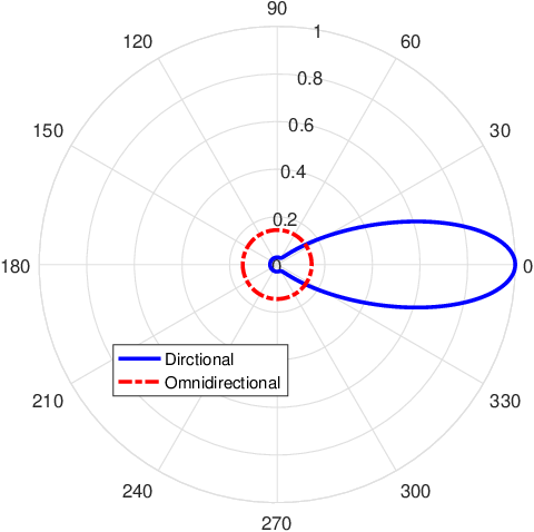
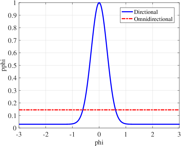
We corroborate our analysis on constrained maximization of ergodic capacity as well as outage probability and SEP derivations with Matlab simulations. To illustrate the advantage of ESPAR antennas on increasing constrained capacity, we compare the performance of our CR system with another CR system in which SU has an omni-directional antenna. Different from an ESPAR antenna that concentrates the electromagnetic power in specific directions (so-called sector or beam), an omni-directional antenna spreads the power equally in all angles. To fairly compare the performance of our CR system (in which SU has an ESPAR antenna) with the other CR system (in which SU has an omni-directional antenna), we let for , i.e., we set the gain of the omni-directional antenna to be . Note that, with this setting, we have the following equality44 4 We note that comparing an ESPAR antenna with the omni-directional antenna obtained from the same ESPAR antenna is not a fair comparison for the following reason. The omni-directional beampattern obtained from the same ESPAR antenna (when reactive loads of all parasitic elements are equal) becomes for . Clearly, this beampattern does not satisfy the equality in (46) and hence the comparison between the two CR systems is not fair.
| (46) |
Fig. 7(a) shows the beampatterns of omni-directional and ESPAR antennas in polar coordinate, where , (corresponding to ). Note that the radius of the red beampattern is and the blue beampattern has the maximum value of at angle radians. The area covered by the solid blue beampattern is equal to the area covered by the dashed red beampattern, in the sense that the equality in (46) holds true. Fig. 7(b) plots the same beampatterns in Cartesian coordinate. For the CR system with the omni-directional antenna at SU, we consider a modified procedure for channel sensing and monitoring, channel training and data transmission phases55 5 Since the omni-directional antenna has only one beampattern, there is no beam selection corresponding to the orientations of PU and SU. Thus, step 1.3 of Table II will be removed. The following steps in Table II are modified: in step 2.2, SU estimates only one channel gain , in step 2.4, SU feeds back only the -bit representation of the index of the quantization interval to which belongs to SU, in step 3.1, SU adapts its discrete power level , using the information received from SU. (with respect to the description in Section II-C) and denote the constrained capacity in (P2) evaluated at the optimized variables , ’s, ’s, by . For our CR system let denote the constrained capacity in (P2), that is evaluated at the optimized variables ’s, ’s. Obviously, the optimized variables obtained from solving (P2) for omni-directional and ESPAR antennas can be different.
| Parameter | Value | Parameter | Value | Parameter | Value |
|---|---|---|---|---|---|
| watts | |||||
| ms | |||||
| dB |
Our simulation parameters are given in Table III. First, we explore the effect of increasing the number of quantization bits . Fig. 8(a) shows and versus for different , when , () , () and (corresponding to ). As a baseline we also plot the capacity when perfect CSI (for SU-SU link) is available for both CR systems (labeled as in the figures). Clearly, our CR system with the ESPAR antenna at SU yields a higher capacity than the CR system with the omni-directional antenna at SU. This figure also shows that as increases, increases and for bits is very close to the baseline capacity. To observe the impact of increasing the number of beams (the number of parasitic elements of the ESPAR antenna), Fig. 8(b) plots and versus for different , when . Comparing Figs. 8(a) and 8(b) we observe that as increases a higher capacity can be achieved.
To explore the effect of changes in PU orientation, Figs. 9(a) and 9(b) illustrate and versus for when and , respectively (with fixed ). Comparing Figs. 8(a), 9(a), 9(b) we observe that as becomes further away from , the imposed interference on PU from SU decreases and SU can transmit at a higher transmit power level, leading to an increase in . Note that in Figs. 8(a), 8(b), 9(a), 9(b) are the same. Let denote that is averaged over all possible and . Fig. 10(a) plots and versus for . Clearly, our CR system with the ESPAR antenna at SU yields a higher capacity on average, compared to the CR system with the omni-directional antenna at SU.
To quantify the capacity improvement provided with the ESPAR antenna, we define the ratio . Fig. 10(b) shows versus for dB and . First, we consider how behaves as increases, for a given value. Fig. 10(b) shows that, as increases from zero to a certain value, decreases. As increases beyond that certain value, increases, however, it becomes constant after reaches a certain point. For instance, given dB, decreases from to , as increases from zero to dB, it increases from to , as increases from dB to dB, and it becomes constant afterward. The reason for this behavior is that, when dB, the average transmit power constraint in (9) is dominant for both ESPAR and omni-directional antennas. For dB dB, the average transmit power constraint is dominant for the ESPAR antenna and the average interference constraint in (34) is dominant for the omni-directional antenna. For dB, the average interference constraint is dominant for both ESPAR and omni-directional antennas. Next, we examine how behaves as decreases, for a given value. Fig. 10(b) shows that, for dB does not vary much as decreases, since the average transmit power constraint is dominant. However, this behavior changes as increases beyond dB, where we note increases as decreases. Overall, we observe that the ESPAR antenna can provide a high capacity improvement ( varies between and in Fig. 10(b)), compared with the omni-directional antenna, and the capacity improvement changes as and vary.


Next, we explore the influence of parameter defined in (16b). Fig. 11 plots and versus for and two choices of : (corresponding to ) and (corresponding to ). We observe that, for a given value, when we increase to , the capacity enhancement for the ESPAR antenna is higher than that of the omni-directional antenna. To explain this observation, let denote the ESPAR beampattern attenuation in side-lobe with respect to its maximum value (main-lobe). Increasing positively affects in two ways. First, the ESPAR antenna can reduce the imposed interference on PU more effectively, and hence SU can transmit at higher power levels, without violating the average interference constraint. Second, SU-SU link becomes a stronger link for data communication. Increasing , however, affects differently. We note that, although increasing renders SU-SU link a stronger link for data communication (positive impact), it increases the imposed interference on PU (negative impact), and hence SU is enforced to transmit at lower power levels to satisfy the average interference constraint.
Let and denote and that are the averaged over all possible and , respectively. For comparison, we also include the outage and symbol error probabilities and corresponding to the CR system that its SU has an omni-directional antenna. Fig. 12(a) illustrates and versus . We observe that given an value, both outage and symbol error probabilities decrease as increases. However, they remain constant as increases beyond a certain point (they reach error floors). These behaviors can be explained as the following. For low , the average transmit power constraint in (9) is dominant and and decrease as increases, since SU can transmit at higher power levels. On the other hand, for high , the average interference constraint in (34) is dominant and SU cannot increase its transmit power level, regardless of how high becomes. As a result, and remain constant. Compared with the ESPAR antenna, the omni-directional antenna imposes a larger interference on PU. Thus, the average interference constraint for the omin-directional antenna becomes active at a smaller value, compared with the ESPAR antenna. As a result both outage and symbol error probabilities reach error floors at smaller values, compared with the ESPAR antenna. Also, we note that as increases decreases. Fig. 12(b) plots and versus . Similar observations to those of Fig. 12(a) can be made here. In a nutshell, Figs. 12(a) and 12(b) show that our proposed CR system yields lower outage and symbol error probabilities, compared with the CR system that its SU has an omni-directional antenna.


VII Conclusions
We proposed a holistic system design for integrated sector-based spectrum sensing and sector-based data communication for an opportunistic CR system consisting of a PU, SU, and SU, where SU is equipped with an ESPAR antenna that has parasitic elements, and there is an error-free bandwidth limited feedback channel from SU to SU. We formulated a constrained optimization problem, where the ergodic capacity for SU-SU link is maximized, subject to average transmit power and interference constraints, and the optimization variables are channel sensing duration, quantization thresholds at SU, and discrete power levels at SU. Our problem formulation takes into consideration the effect of imperfect spectrum sensing, the error in determining the true orientation of PU, the error in selecting the strongest channel for data communication, and the impact of channel gain quantization. We developed an iterative suboptimal algorithm with a low computational complexity, based on the BCDA, that finds a unique and locally optimal solution for the constrained problem. In addition, we derived closed form expressions for outage and symbol error probabilities of our opportunistic CR system. We corroborated our mathematical analyses with extensive simulations. Our numerical results demonstrate that our proposed CR system with the ESPAR antenna at SU yields a significantly higher capacity, a lower outage probability, and a lower symbol error probability, compared with a CR system that its SU has an omni-directional antenna. The capacity improvement varies as the average transmit power and average interference constraints change. For instance, at dB, dB, the capacity of our CR system is times larger than the capacity of the CR system with omni-directional antenna. Furthermore, we showed that with only a small number of feedback bits the capacity of our CR system approaches to its baseline, which assumes the full knowledge of unquantized channel gain.
References
- [1] H. Yazdani and A. Vosoughi, “On the spectrum sensing, beam selection and power allocation in cognitive radio networks using reconfigurable antennas,” in 2019 53nd Annual Conference on Information Sciences and Systems (CISS), March 2019.
- [2] T. Yucek and H. Arslan, “A survey of spectrum sensing algorithms for cognitive radio applications,” IEEE Communications Surveys Tutorials, vol. 11, no. 1, pp. 116–130, First 2009.
- [3] H. Zhang, Y. Nie, J. Cheng, V. C. M. Leung, and A. Nallanathan, “Sensing time optimization and power control for energy efficient cognitive small cell with imperfect hybrid spectrum sensing,” IEEE Transactions on Wireless Communications, vol. 16, no. 2, pp. 730–743, Feb 2017.
- [4] H. Hu, H. Zhang, and Y. C. Liang, “On the spectrum- and energy-efficiency tradeoff in cognitive radio networks,” IEEE Transactions on Communications, vol. 64, no. 2, pp. 490–501, Feb 2016.
- [5] G. Ozcan, M. C. Gursoy, N. Tran, and J. Tang, “Energy-efficient power allocation in cognitive radio systems with imperfect spectrum sensing,” IEEE Journal on Selected Areas in Communications, vol. 34, no. 12, pp. 3466–3481, Dec 2016.
- [6] P. Paysarvi-Hoseini and N. C. Beaulieu, “Optimal wideband spectrum sensing framework for cognitive radio systems,” IEEE Transactions on Signal Processing, vol. 59, no. 3, pp. 1170–1182, March 2011.
- [7] G. Ozcan, M. C. Gursoy, N. Tran, and J. Tang, “Energy-efficient power allocation in cognitive radio systems with imperfect spectrum sensing,” IEEE Journal on Selected Areas in Communications, vol. 34, no. 12, pp. 3466–3481, Dec 2016.
- [8] M. Shirazi, T. Li, J. Huang, and X. Gong, “A reconfigurable dual-polarization slot-ring antenna element with wide bandwidth for array applications,” IEEE Transactions on Antennas and Propagation, vol. 66, no. 11, pp. 5943–5954, Nov 2018.
- [9] M. Shirazi, J. Huang, T. Li, and X. Gong, “A switchable-frequency slot-ring antenna element for designing a reconfigurable array,” IEEE Antennas and Wireless Propagation Letters, vol. 17, no. 2, pp. 229–233, Feb 2018.
- [10] M. A. Almasi, H. Mehrpouyan, V. Vakilian, N. Behdad, and H. Jafarkhani, “A new reconfigurable antenna MIMO architecture for mmWave communication,” in 2018 IEEE International Conference on Communications (ICC), May 2018, pp. 1–7.
- [11] H. Yazdani, A. Vosoughi, and N. Rahnavard, “Compressive sensing based direction-of-arrival estimation using reweighted greedy block coordinate descent algorithm for ESPAR antennas,” in MILCOM 2017 - 2017 IEEE Military Communications Conference (MILCOM), Oct 2017, pp. 169–173.
- [12] W. Ouyang and X. Gong, “A cavity-backed slot ESPAR E-plane array,” in 2017 IEEE 18th Wireless and Microwave Technology Conference (WAMICON), April 2017, pp. 1–3.
- [13] D. Wilcox, E. Tsakalaki, A. Kortun, T. Ratnarajah, C. B. Papadias, and M. Sellathurai, “On spatial domain cognitive radio using single-radio parasitic antenna arrays,” IEEE Journal on Selected Areas in Communications, vol. 31, no. 3, pp. 571–580, March 2013.
- [14] A. M. Alaa, M. H. Ismail, and H. Tawfik, “Random aerial beamforming for underlay cognitive radio with exposed secondary users,” IEEE Transactions on Vehicular Technology, vol. 65, no. 7, pp. 5364–5383, July 2016.
- [15] R. Qian and M. Sellathurai, “On the implementation of blind interference alignment with single-radio parasitic antennas,” IEEE Transactions on Vehicular Technology, vol. 65, no. 12, pp. 10 180–10 184, Dec 2016.
- [16] M. A. et al., “Enhancing LTE with cloud-RAN and load-controlled parasitic antenna arrays,” IEEE Communications Magazine, vol. 54, no. 12, pp. 183–191, December 2016.
- [17] Z. Bouida, H. El-Sallabi, A. Ghrayeb, and K. A. Qaraqe, “Reconfigurable antenna-based space-shift keying (SSK) for MIMO Rician channels,” IEEE Transactions on Wireless Communications, vol. 15, no. 1, pp. 446–457, Jan 2016.
- [18] Z. Bouida, H. El-Sallabi, M. Abdallah, A. Ghrayeb, and K. A. Qaraqe, “Reconfigurable antenna-based space-shift keying for spectrum sharing systems under Rician fading,” IEEE Transactions on Communications, vol. 64, no. 9, pp. 3970–3980, Sept 2016.
- [19] R. Senanayake, P. J. Smith, P. A. Martin, and J. S. Evans, “Performance analysis of reconfigurable antenna arrays,” IEEE Transactions on Communications, vol. 65, no. 6, pp. 2726–2739, June 2017.
- [20] C. Liu and M. Jin, “Maximum-minimum spatial spectrum detection for cognitive radio using parasitic antenna arrays,” in 2014 IEEE/CIC International Conference on Communications in China (ICCC), Oct 2014, pp. 365–369.
- [21] R. Qian, M. Sellathurai, and T. Ratnarajah, “Directional spectrum sensing for cognitive radio using ESPAR arrays with a single RF chain,” in 2014 European Conference on Networks and Communications (EuCNC), June 2014, pp. 1–5.
- [22] C. Liu, M. Li, and M. L. Jin, “Blind energy-based detection for spatial spectrum sensing,” IEEE Wireless Communications Letters, vol. 4, no. 1, pp. 98–101, Feb 2015.
- [23] T. Wu and H. C. Yang, “Performance analysis for RUB-based cognitive radio network with cooperative beam selection,” in 2014 IEEE 80th Vehicular Technology Conference (VTC2014-Fall), Sept 2014, pp. 1–5.
- [24] M. Sayed, M. Abdallah, K. Qaraqe, K. Tourki, and M. S. Alouini, “Joint opportunistic beam and spectrum selection schemes for spectrum sharing systems with limited feedback,” IEEE Transactions on Vehicular Technology, vol. 63, no. 9, pp. 4408–4421, Nov 2014.
- [25] M. Abdallah, M. Sayed, M. S. Alouini, and K. A. Qaraqe, “Interference-aware random beam selection for spectrum sharing systems,” in 2012 IEEE Vehicular Technology Conference (VTC Fall), Sept 2012, pp. 1–5.
- [26] T. Q. Wu, H. C. Yang, and Y. C. Liang, “Cooperative secondary beam selection for cognitive multiuser MIMO transmission with random beamforming,” IEEE Transactions on Cognitive Communications and Networking, vol. 2, no. 2, pp. 141–149, June 2016.
- [27] P. J. Smith, A. Firag, P. A. Martin, and R. Murch, “SNR performance analysis of reconfigurable antennas,” IEEE Communications Letters, vol. 16, no. 4, pp. 498–501, April 2012.
- [28] M. H. Yılmaz, M. M. Abdallah, H. M. El-Sallabi, J. F. Chamberland, K. A. Qaraqe, and H. Arslan, “Joint subcarrier and antenna state selection for cognitive heterogeneous networks with reconfigurable antennas,” IEEE Transactions on Communications, vol. 63, no. 11, pp. 4015–4025, Nov 2015.
- [29] A. Abdalrazik, H. Soliman, M. F. Abdelkader, and T. M. Abuelfadl, “Power performance enhancement of underlay spectrum sharing using microstrip patch ESPAR antenna,” in 2016 IEEE Wireless Communications and Networking Conference, April 2016, pp. 1–6.
- [30] C. Sun, A. Hirata, T. Ohira, and N. C. Karmakar, “Fast beamforming of electronically steerable parasitic array radiator antennas: theory and experiment,” IEEE Transactions on Antennas and Propagation, vol. 52, no. 7, pp. 1819–1832, July 2004.
- [31] R. Qian, M. Sellathurai, and D. Wilcox, “A study on MVDR beamforming applied to an ESPAR antenna,” IEEE Signal Processing Letters, vol. 22, no. 1, pp. 67–70, Jan 2015.
- [32] H. Du, Y. Sun, and Z. Wu, “Robust beamforming for ESPAR-based cognitive radio MIMO system,” in 2017 IEEE/CIC International Conference on Communications in China (ICCC), Oct 2017, pp. 1–5.
- [33] H. Yazdani and A. Vosoughi, “On cognitive radio systems with directional antennas and imperfect spectrum sensing,” in 2017 IEEE International Conference on Acoustics, Speech and Signal Processing (ICASSP), March 2017, pp. 3589–3593.
- [34] ——, “On the combined effect of directional antennas and imperfect spectrum sensing upon ergodic capacity of cognitive radio systems,” in 2017 51st Asilomar Conference on Signals, Systems, and Computers, Oct 2017, pp. 1702–1706.
- [35] H. Yazdani and A. Vosoughi, “On optimal sensing and capacity trade-off in cognitive radio systems with directional antennas,” in 2018 IEEE Global Conference on Signal and Information Processing (GlobalSIP), Nov 2018, pp. 1015–1019.
- [36] J. Werner, J. Wang, A. Hakkarainen, D. Cabric, and M. Valkama, “Performance and Cramér–Rao bounds for DoA/RSS estimation and transmitter localization using sectorized antennas,” IEEE Transactions on Vehicular Technology, vol. 65, no. 5, pp. 3255–3270, May 2016.
- [37] M. M. Abdallah, A. H. Salem, M. S. Alouini, and K. A. Qaraqe, “Adaptive discrete rate and power transmission for spectrum sharing systems,” IEEE Transactions on Wireless Communications, vol. 11, no. 4, pp. 1283–1289, April 2012.
- [38] X. Guo, Y. He, S. Atapattu, S. Dey, and J. S. Evans, “Power allocation for distributed detection systems in wireless sensor networks with limited fusion center feedback,” IEEE Transactions on Communications, vol. 66, no. 10, pp. 4753–4766, Oct 2018.
- [39] A. Goldsmith, Wireless Communications. Cambridge University Press, 2005.
- [40] T. M. Cover and J. A. Thomas, Elements of Information Theory (Wiley Series in Telecommunications and Signal Processing). New York, NY, USA: Wiley-Interscience, 2006.