$b\to s\ell^{+}\ell^{-}$ Transitions in Two-Higgs-Doublet ModelsPreprint: PSI-PR-19-02, ZU-TH 10/19

Andreas Crivellin Affiliation: Paul Scherrer Institut, CH–5232 Villigen PSI, Switzerland Affiliation: Physik-Institut, Universität Zürich, Winterthurerstrasse 190, CH-8057 Zürich, Switzerland Email: andreas.crivellin@psi.ch Dario Müller Affiliation: Paul Scherrer Institut, CH–5232 Villigen PSI, Switzerland Affiliation: Physik-Institut, Universität Zürich, Winterthurerstrasse 190, CH-8057 Zürich, Switzerland Email: dario.mueller@psi.ch Christoph Wiegand Affiliation: Albert Einstein Center for Fundamental Physics, Institute for Theoretical Physics, University of Bern, CH-3012 Bern, Switzerland Email: wiegand@itp.unibe.ch

Abstract

In this article we study $b\to s\mu^{+}\mu^{-}$ transitions and possible correlations with the anomalous magnetic moment of the muon ( $a_{\mu}$ ) within two-Higgs-doublet models with generic Yukawa couplings, including the possibility of right-handed neutrinos. We perform the matching on the relevant effective Hamiltonian and calculate the leading one-loop effects for $b\to s\ell\ell^{(\prime)}$ , $b\to s\gamma$ , $\Delta B=\Delta S=2$ , $b\to s\nu\bar{\nu}$ and $\ell\to\ell^{\prime}\gamma$ transitions in a general $R_{\xi}$ gauge. Concerning the phenomenology, we find that an explanation of the hints for new physics in $b\to s\mu^{+}\mu^{-}$ data is possible once right-handed neutrinos are included. If lepton flavour violating couplings are allowed, one can account for the discrepancy in $a_{\mu}$ as well. However, only a small portion of parameter space gives a good fit to $b\to s\mu^{+}\mu^{-}$ data and the current bound on $h\to\tau\mu$ requires the mixing between the neutral Higgses to be very small if one aims at an explanation of $a_{\mu}$ .

1 Introduction

Two-Higgs-doublet models (2HDMs) Lee:1973iz have been under intensive investigation for a long time (see e.g. Ref. Gunion:1989we for an introduction or Ref. Branco:2011iw for a review article). There are several reasons for this intense interest: First of all, 2HDMs are extremely simple extensions of the Standard Model (SM) obtained by adding a single scalar $SU(2)_{L}$ doublet to the SM particle content. Furthermore, motivation for 2HDMs comes from axion models Kim:1986ax because a possible CP violating QCD-theta term can be absorbed Peccei:1977hh if the Lagrangian possesses a global $U(1)$ symmetry. This is only possible if the SM is extended by at least one Higgs doublet. Also the baryon asymmetry of the universe can be generated within 2HDMs while the amount of CP violation in the SM alone is too small to achieve this Trodden:1998qg. Finally, the Minimal Supersymmetric Standard Model predicts the presence of a second Higgs doublet Haber:1984rc, due to the holomorphicity of the superpotential. The effective theory obtained after integrating out the superpartners of the SM particles (sfermions, gaugions and higgsinos) is a 2HDM (with the addition of higher dimensional operators involving two Higgs doublets Crivellin:2016ihg).

2HDMs possess three additional physical scalars with respect to the single Higgs boson of the SM; a neutral CP-even $H^{0}$ , a CP-odd scalar $A^{0}$ and a charged scalar $H^{\pm}$ (under the assumption of CP conservation). These new particles are not only interesting with respect to direct searches at the LHC (see e.g. Ref. Bhatia:2017ttp; Arbey:2017gmh; Basler:2017nzu; Haisch:2017gql; Jenniches:2018zlb; Chen:2018uim; Enberg:2018pye; Arhrib:2018ewj; Hanson:2018uhf for recent reports). In addition, they give rise to important effects in low-energy precision flavour observables, providing a complementary window to physics beyond the SM. In this respect, decays of neutral mesons to charged lepton pairs (e.g. $B_{s(d)}\to\mu^{+}\mu^{-}$ , $D\to\mu^{+}\mu^{-}$ and $K_{L}\to\mu^{+}\mu^{-}$ ) are very interesting because they are especially sensitive to scalar operators which possess enhanced matrix elements with respect to vector operators. For this reason, $B_{s}\to\mu^{+}\mu^{-}$ (which can be calculated more precisely than $D\to\mu^{+}\mu^{-}$ or $K_{L}\to\mu^{+}\mu^{-}$ and has a larger branching fraction than $B_{d}\to\mu^{+}\mu^{-}$ ) has been studied frequently in the context of 2HDMs. However, the focus was on models with natural flavour conservation (i.e. with a $\mathds{Z}_{2}$ symmetry in the Yukawa sector) He:1988tf; Skiba:1992mg; Dai:1996vg; Huang:1998bf; Logan:2000iv; Cheng:2015yfu; Arnan:2017lxi, alignment Iltan:2000ck; Li:2014fea or generic flavour violation in the down sector Mahmoudi:2009zx; Buras:2010mh; Crivellin:2013wna; Crivellin:2017upt. In all these setups, the dominant effect originates from scalar operators. The current measurement of $B_{s}\to\mu^{+}\mu^{-}$ Amhis:2016xyh (by ATLAS, CMS and LHCb CMS:2014xfa; Aaij:2013aka; Chatrchyan:2013bka; Aaboud:2018mst)

{\rm Br}[B_{s}\to\mu^{+}\mu^{-}]_{\rm EXP}=(3.1\pm 0.7)\times 10^{-9}\,,

(1)

agrees quite well with the SM prediction Bobeth:2013uxa; Beneke:2017vpq

{\rm Br}[B_{s}\to\mu^{+}\mu^{-}]_{\rm SM}=(3.57\pm 0.17)\times 10^{-9}\,.

(2)

This puts stringent constraints on 2HDMs with scalar operators contributing to $b\to s\mu^{+}\mu^{-}$ transitions. Furthermore, LHCb found significant hints for new physics in $b\to s\ell^{+}\ell^{-}$ data, showing a coherent pattern of deviations from the SM predictions with a significance of more than $4$ – $5\,\sigma$ Capdevila:2017bsm; Alguero:2019ptt¹¹ 1 Including only $R(K)$ and $R(K^{*})$ , the significance is at the 4 $\,\sigma$ level Altmannshofer:2017yso; DAmico:2017mtc; Geng:2017svp; Ciuchini:2017mik; Hiller:2017bzc; Hurth:2017hxg; Ciuchini:2019usw.. However, in order to explain these anomalies, vector operators, in particular $O_{9}$ , are necessary while an explanation of the anomalies with scalar operators alone is not possible.

Within 2HDMs, vector operators at the dimension 6 level can only be generated via loop effects. However, contributions to other loop-induced processes such as $b\to s\gamma$ (for which the SM prediction Misiak:2015xwa is in very well agreement with the experimental average Amhis:2016xyh), $b\to s\nu\bar{\nu}$ , (where the experimental upper bound Grygier:2017tzo; Lees:2013kla approaches the SM prediction Buras:2014fpa) or $B_{s}-\bar{B}_{s}$ mixing Amhis:2016xyh unavoidably arise and their constraints must be taken into account. Therefore, an explanation of $b\to s\ell^{+}\ell^{-}$ data in the context of multi-Higgs-doublet models might require the introduction of right-handed neutrinos Li:2018rax; Marzo:2019ldg. Furthermore, any model with sizeable couplings to muons could potentially address the long-lasting discrepancy between experiment Bennett:2006fi and the SM prediction²² 2 The SM prediction of $a_{\mu}$ is currently re-evaluated in a community-wide effort prompted by upcoming improved measurements at Fermilab Grange:2015fou and J-PARC Saito:2012zz (see also Gorringe:2015cma). With electroweak Czarnecki:1995wq; Czarnecki:1995sz; Gnendiger:2013pva and QED Aoyama:2017uqe contributions under good control, recent advances in the evaluation of the hadronic part include: hadronic vacuum polarization DellaMorte:2017dyu; Davier:2017zfy; Borsanyi:2017zdw; Blum:2018mom; Keshavarzi:2018mgv; Giusti:2018mdh; Colangelo:2018mtw, hadronic light-by-light scattering Gerardin:2016cqj; Blum:2016lnc; Colangelo:2017qdm; Colangelo:2017fiz; Blum:2017cer; Hoferichter:2018dmo, and higher-order hadronic corrections Kurz:2014wya; Colangelo:2014qya.

\Delta a_{\mu}=a_{\mu}^{\text{EXP}}-a_{\mu}^{\text{SM}}\sim 270(85)\times 10^{-11}\,,

(3)

of $3$ – $4\,\sigma$ . For definiteness, and in order to be conservative, we choose a value at the lower end. In the case of lepton flavour violation, $a_{\mu}$ is intrinsically correlated to lepton flavour violating decays such as $\tau\to\mu\gamma$ whose bound must be taken into account. Furthermore, in 2HDMs also $h\to\tau\mu$ gives relevant bounds due to the mixing between the neutral CP-even Higgses.

In this article we want to investigate $b\to s\mu^{+}\mu^{-}$ transitions within 2HDMs in the light of the corresponding hints for new physics and its correlations with other $b\to s$ transitions and $a_{\mu}$ . For this purpose, we will consider a 2HDM with a CP conserving Higgs potential but with generic sources of flavour violation and the possible addition of right-handed neutrinos. After establishing our conventions in Sec. 2, we will use this setup to calculate the tree-level matching on the effective Hamiltonian governing $b\to s$ transitions and the leading one-loop effects in Sec. 3. Section 4 is devoted to the calculation of the matching on the $\Delta B=\Delta S=2$ Hamiltonian, to $a_{\mu}$ , $h\to\tau\mu$ and $b\to s\nu\bar{\nu}$ . In our phenomenological analysis in Sec. 5 we will address the question if the hints for new physics in $b\to s\mu^{+}\mu^{-}$ transitions can be explained within 2HDMs without violating the bounds from other processes, before we conclude in Sec. 6.

2 Model and Conventions

$\rm{Type}$	${c_{y}^{d}}$	${c_{y}^{u}}$	${c_{y}^{\ell}}$	${c_{\tilde{\varepsilon}}^{d}}$	${c_{\tilde{\varepsilon}}^{u}}$	${c_{\tilde{\varepsilon}}^{\ell}}$
I	${\cot\left(\beta\right)}$	${\cot\left(\beta\right)}$	${\cot\left(\beta\right)}$	${-\sin\left(\beta\right)}$	${-\sin\left(\beta\right)}$	${-\sin\left(\beta\right)}$
II	${-\tan\left(\beta\right)}$	${\cot\left(\beta\right)}$	${-\tan\left(\beta\right)}$	${\cos\left(\beta\right)}$	${-\sin\left(\beta\right)}$	${\cos\left(\beta\right)}$
X	${\cot\left(\beta\right)}$	${\cot\left(\beta\right)}$	${-\tan\left(\beta\right)}$	${-\sin\left(\beta\right)}$	${-\sin\left(\beta\right)}$	${\cos\left(\beta\right)}$
Y	${-\tan\left(\beta\right)}$	${\cot\left(\beta\right)}$	${\cot\left(\beta\right)}$	${\cos\left(\beta\right)}$	${-\sin\left(\beta\right)}$	${-\sin\left(\beta\right)}$

Table 1: Relations between the parameters

\varepsilon_{ij}^{F}

of the Higgs basis and the new parameters

\tilde{\varepsilon}^{F}_{ij}

in one of the other four bases with

\varepsilon_{ij}^{F}=c_{y}^{F}y^{f}_{i}\delta_{ij}+\tilde{\varepsilon}^{F}_{ij}/c_{\tilde{\varepsilon}}^{F}

. The

\tilde{\varepsilon}^{F}_{ij}

break the

\mathds{Z}_{2}

symmetry of the four 2HDMs with natural flavour conservation and induce flavour changing neutral currents.

As outlined in the introduction, we supplement the SM by a second scalar doublet with the same hypercharge as the first one. For the calculation of flavour observables it is convenient to work in the Higgs basis Georgi:1978ri; Lavoura:1994fv; Botella:1994cs where only one Higgs doublet acquires a vacuum expectation value and therefore the generation of the fermions and gauge boson masses is separated from the couplings to fermions. Using the notation of Ref. Davidson:2016utf, we have

\displaystyle\Phi_{1}=\begin{pmatrix}G^{+}\\ \dfrac{v+H_{1}^{0}+iG^{0}}{\sqrt{2}}\end{pmatrix},

\displaystyle\Phi_{2}=\begin{pmatrix}H^{+}\\ \dfrac{H_{2}^{0}+iA^{0}}{\sqrt{2}}\end{pmatrix},

(4)

with $v\simeq 246$ GeV. $G^{+}$ and $G^{0}$ are the Goldstone bosons and $A^{0}$ denotes the physical CP-odd scalar, assuming that CP is conserved in the Higgs potential. The CP-even mass eigenstates are

\displaystyle\begin{split}h^{0}&=H_{1}^{0}\sin(\beta-\alpha)+H_{2}^{0}\cos(\beta-\alpha)\,,\\ H^{0}&=H_{1}^{0}\cos(\beta-\alpha)-H_{2}^{0}\sin(\beta-\alpha)\,,\end{split}

(5)

where we defined the mixing angle as $\beta-\alpha$ for easier comparison with the well-known type-I/II/X/Y 2HDMs. In the following, we will abbreviate $s_{\beta\alpha}\equiv\sin(\beta-\alpha)$ and $c_{\beta\alpha}\equiv\cos(\beta-\alpha)$ and assume that $h^{0}$ is the SM-like Higgs boson with a mass of around 125 GeV. We require $c_{\beta\alpha}$ to be small (at most $\mathcal{O}(0.1)$ ) such that its properties are compatible with experiments Sirunyan:2018koj; ATLAS:2018doi. With these conventions the couplings of the scalar bosons to fermions are given by

\displaystyle\begin{split}{L_{Y}}&=-\!\!\!\sum\limits_{F=u,d,\ell,\nu}\bigg[{{\bar{F}}_{f}}\Big(\,{\dfrac{{m_{f}^{F}}}{v}{\delta_{fi}}c_{\beta\alpha}\!-\!\left({\varepsilon_{fi}^{F}{P_{R}}+\varepsilon_{if}^{F*}{P_{L}}}\right)\!s_{\beta\alpha}}\Big)\!{F_{i}}{H^{0}}\\ &\phantom{-\sum\limits_{F=u,d,\ell,\nu}\bigg[}+{{\bar{F}}_{f}}\Big(\,{\dfrac{{m_{f}^{F}}}{v}{\delta_{fi}}s_{\beta\alpha}\!+\!\left({\varepsilon_{fi}^{F}{P_{R}}+\varepsilon_{if}^{F*}{P_{L}}}\right)\!c_{\beta\alpha}}\Big)\!{F_{i}}{h^{0}}\\ &\phantom{-\sum\limits_{F=u,d,\ell,\nu}\bigg[}+i{\eta_{F}}{{\bar{F}}_{f}}\!\left({\varepsilon_{fi}^{F}{P_{R}}-\varepsilon_{if}^{F*}{P_{L}}}\right)\!{F_{i}}{A^{0}}\bigg]\\ &-\!\sqrt{2}\Big[{{{\bar{u}}_{f}}\!\left({V_{fj}\varepsilon_{ji}^{d}{P_{R}}\!-\!\varepsilon_{jf}^{u*}V_{ji}{P_{L}}}\right)\!{d_{i}}{H^{+}}\!+\!{{\bar{\nu}}_{f}}\!\left({U_{jf}^{{\rm{*}}}\varepsilon_{ji}^{\ell}{P_{R}}\!-\!\varepsilon_{jf}^{\nu*}U_{ij}^{{\rm{*}}}{P_{L}}}\right)\!{\ell_{i}}{H^{+}}\!+\!{\rm h.c.}}\Big].\end{split}

(6)

$V$ ( $U$ ) is the CKM (PMNS) matrix, $m_{i}^{F}$ is the mass of the fermion $F=\{u,d,\ell,\nu\}$ with flavour index $i$ and

-\eta_{u}=-\eta_{\nu}=\eta_{\ell}=\eta_{d}=1\,.

(7)

We also allowed for the presence of right-handed neutrinos $N$ with a Majorana mass term $-1/2M\bar{N}^{c}N$ . This manifests itself in Eq. (6) through the terms $m^{\nu}$ and $\varepsilon^{\nu}$ which otherwise would be absent. Note that $m^{\nu}$ corresponds to the Dirac mass term of the neutrinos which is related to the physical neutrino mass via the see-saw mechanism. Assuming a mass scale of the right-handed neutrinos at the TeV scale requires $m^{\nu}$ to be at most around 10 MeV. Thus we can safely neglect its effect on the Higgs couplings to fermions and focus on $\varepsilon^{\nu}$ which is decoupled from the neutrino masses and thus unconstrained.

We do not need to discuss the Higgs potential in detail since, in addition to the physical masses and mixing angles, only the two Higgs self-couplings enter in our calculation in the case of CP conservation. We will simply parametrize these couplings as $\lambda_{h_{0}H^{+}H^{-}}$ and $\lambda_{H_{0}H^{+}H^{-}}$ and refer the interested reader to Eq. (78) in the appendix for the explicit expressions.

The Higgs basis defined in Eq. (6) is useful for calculations and phenomenology since fermion masses (generated from electroweak symmetry breaking) and the additional free couplings are decoupled. However, this basis is not motivated by a $\mathds{Z}_{2}$ symmetry which is capable to provide protection against flavour changing neutral currents. However, the parameters $\varepsilon^{F}_{ij}$ in the Higgs basis can be related to the ones within the four 2HDMs with natural flavour conservation (type-I/II/X/Y) as

\varepsilon_{ij}^{F}=c_{y}^{F}\dfrac{m_{i}^{F}}{v}\delta_{ij}+\frac{\tilde{\varepsilon}^{F}_{ij}}{c_{\tilde{\varepsilon}}^{F}}\,.

(8)

The $\tilde{\varepsilon}^{F}_{ij}$ are the flavour changing entries in the new basis, i.e. the corrections to natural flavour conservation. The coefficients $c_{y}^{f}$ and $c_{\tilde{\varepsilon}}^{F}$ are given in Table 1. In this basis, the terms $\tilde{\varepsilon}^{F}_{ij}$ break the $\mathds{Z}_{2}$ symmetry and lead to deviations from natural flavour conservation.

\begin{overpic}[tree-level.pdf] \put(12.0,33.0){$b$} \put(12.0,3.0){$s$} \put(38.0,23.0){$H^{0},h^{0},A^{0}$} \put(81.0,33.0){$\ell$} \put(81.0,3.0){$\ell^{\prime}$} \end{overpic}

Figure 1: Tree-level effects in

b\to s\ell^{+}\ell^{-}

transitions induced by the flavour-changing couplings

\varepsilon^{d}_{23,32}

. These diagrams contribute to the Wilson coefficients of scalar operator

C_{S,P}^{(\prime)IJ}

as given in Eq. (13).

3 $b\to s\ell^{+}\ell^{-}$ Processes

We define the effective Hamiltonian giving direct effects in $b\to s\ell\ell^{(\prime)}$ and $b\to s\gamma$ transitions as

\displaystyle H_{\rm eff}^{{\ell_{I}}{\ell_{J}}}

\displaystyle=

\displaystyle-\dfrac{{4{G_{F}}}}{{\sqrt{2}}}{V_{tb}}V_{ts}^{*}\left(\sum\limits_{K=7,8}{C_{K}^{(\prime)}O_{K}^{(\prime)}}+\sum\limits_{K=9,10,S,P}{C_{K}^{(\prime)IJ}O_{K}^{(\prime)IJ}}\right)\,,

(9)

with the operators

\displaystyle\begin{aligned} O_{7}&=\dfrac{{{e}}}{{16{\pi^{2}}}}m_{b}\bar{s}{\sigma^{\mu\nu}}{P_{R}}bF_{\mu\nu}\,,&&&O_{8}&=\dfrac{{{g_{s}}}}{{16{\pi^{2}}}}m_{b}\bar{s}{\sigma^{\mu\nu}}T^{a}{P_{R}}bG_{\mu\nu}^{a}\,,\\ O_{9}^{IJ}&=\dfrac{{{e^{2}}}}{{16{\pi^{2}}}}\bar{s}{\gamma_{\mu}}{P_{L}}b{{\bar{\ell}}_{I}}{\gamma^{\mu}}{\ell_{J}}\,,&&&O_{10}^{IJ}&=\dfrac{{{e^{2}}}}{{16{\pi^{2}}}}\bar{s}{\gamma_{\mu}}{P_{L}}b{{\bar{\ell}}_{I}}{\gamma^{\mu}}{\gamma_{5}}{\ell_{J}}\,,\\ O_{S}^{IJ}&=\dfrac{{{e^{2}}}}{{16{\pi^{2}}}}\bar{s}{P_{L}}b{{\bar{\ell}}_{I}}{\ell_{J}}\,,&&&O_{P}^{IJ}&=\dfrac{{{e^{2}}}}{{16{\pi^{2}}}}\bar{s}{P_{L}}b{{\bar{\ell}}_{I}}{\gamma_{5}}{\ell_{J}}\,,\end{aligned}

(10)

plus their primed counterparts which are obtained by exchanging $P_{L}$ and $P_{R}$ . We did not include tensor operators here since they are not generated at the dim-6 level.

In addition, we include four-quark operators which are generated by charged Higgs exchange (analogous to $O_{2}$ in the SM)

\displaystyle H_{\rm eff}^{sccb}

\displaystyle=-\dfrac{{4{G_{F}}}}{{\sqrt{2}}}{V_{tb}}V_{ts}^{*}\!\!\!\!\!\!\!\!\!\!\sum\limits_{K=\{LL,LR,RL,RR\}}^{5}\!\!\!\!\!\!\!\!\!\!\!\!\!C_{K}O_{K},

(11)

which can contribute to $b\to s\ell^{+}\ell^{-}$ processes at the loop-level. The operators are defined as

\displaystyle\begin{aligned} O_{AB}&=\left({{\bar{s}}}{P_{A}}c\right)\left(\bar{c}{P_{B}}b\right)\,,\end{aligned}

(12)

with $A,B=L,R$ and the colour indices are contracted within the bilinears.

3.1 Tree-Level

At tree-level, in the approximation of vanishing external momenta, we only get contributions to semi-leptonic scalar and pseudoscalar operators from neutral Higgs exchange (see Fig. 1). They are given by

\displaystyle\begin{split}C_{S}^{IJ}=&\frac{16\pi^{2}}{g_{2}^{4}s_{W}^{2}V_{tb}V_{ts}^{*}}\dfrac{m_{W}^{2}}{m_{H^{\pm}}^{2}}\varepsilon_{32}^{d*}\bigg(2s_{\beta\alpha}c_{\beta\alpha}\dfrac{m_{I}^{\ell}\delta_{IJ}}{v}(y_{h}-y_{H})+L_{+}^{IJ}\bigg)\,,\\ C_{P}^{IJ}=&\frac{16\pi^{2}}{g_{2}^{4}s_{W}^{2}V_{tb}V_{ts}^{*}}\dfrac{m_{W}^{2}}{m_{H^{\pm}}^{2}}\varepsilon_{32}^{d*}\bigg(\big(c_{\beta\alpha}^{2}y_{h}+s_{\beta\alpha}^{2}y_{H}\big)\big(\varepsilon_{IJ}^{\ell}-\varepsilon_{JI}^{\ell*}\big)+y_{A}\big(\varepsilon_{IJ}^{\ell}+\varepsilon_{JI}^{\ell*}\big)\bigg)\,,\\ C_{S}^{\prime IJ}=&\frac{16\pi^{2}}{g_{2}^{4}s_{W}^{2}V_{tb}V_{ts}^{*}}\dfrac{m_{W}^{2}}{m_{H^{\pm}}^{2}}\varepsilon_{23}^{d}\bigg(2s_{\beta\alpha}c_{\beta\alpha}\dfrac{m_{I}^{\ell}\delta_{IJ}}{v}\big(y_{h}-y_{H}\big)-L_{-}^{IJ}\bigg)\,,\\ C_{P}^{\prime IJ}=&\frac{16\pi^{2}}{g_{2}^{4}s_{W}^{2}V_{tb}V_{ts}^{*}}\dfrac{m_{W}^{2}}{m_{H^{\pm}}^{2}}\varepsilon_{23}^{d}\bigg(\big(c_{\beta\alpha}^{2}y_{h}+s_{\beta\alpha}^{2}y_{H}\big)\big(\varepsilon_{IJ}^{\ell}-\varepsilon_{JI}^{\ell*}\big)-y_{A}\big(\varepsilon_{IJ}^{\ell}+\varepsilon_{JI}^{\ell*}\big)\bigg)\,,\end{split}

(13)

where we defined

\displaystyle\begin{split}L_{\pm}^{IJ}=y_{A}\big(\varepsilon^{\ell}_{IJ}-\varepsilon^{\ell*}_{JI}\big)\pm\left(c_{\beta\alpha}^{2}y_{h}+s_{\beta\alpha}^{2}y_{H}\right)\big(\varepsilon^{\ell}_{IJ}+\varepsilon^{\ell*}_{JI}\big)\,,\end{split}

(14)

and

\displaystyle y_{A}=\dfrac{m_{H^{\pm}}^{2}}{m_{A_{0}}^{2}}\,,~~~~y_{h}=\dfrac{m_{H^{\pm}}^{2}}{m_{h_{0}}^{2}}\,,~~~~y_{H}=\dfrac{m_{H^{\pm}}^{2}}{m_{H_{0}}^{2}}\,.

(15)

In addition, we define for future convenience the squared mass ratios for heavy Majorana neutrino, up-type quark and the $W$ boson with respect to the charged Higgs

\displaystyle x_{i}=\frac{m_{N_{i}}^{2}}{m_{H^{\pm}}^{2}}\,,~~~~z_{i}=\frac{m_{u_{i}}^{2}}{m_{H^{\pm}}^{2}}\,,~~~~y=\frac{m_{W}^{2}}{m_{H^{\pm}}^{2}}\,.

(16)

We derived Eq. (13) by working at leading order in the external momenta (which we will also do for all following results). This corresponds to an expansion in $m_{b,s}$ and $m_{\ell}$ over the Higgs masses which we assume to be at least at the EW scale. For consistency, one has to take into account all masses $m_{b,s}$ and $m_{\ell}$ in this expansion, also the ones entering via Higgs couplings³³ 3 Note that it is a convenient feature of the Higgs basis that only the couplings which are related to EW symmetry breaking contain fermion masses (unlike in type-I/II/X/Y). Thus one can directly expand in these parameters without taking into account factors of $\sin\alpha$ , $\tan\beta$ , etc.. Equation (13) contains terms linear in light fermion masses which therefore correspond to dim-7 contributions. However, since from the expansion in the external momenta no dim-7 terms arise (the next non-vanishing order is dim-8), it is consistent to keep these terms even though in the loop effects, to be studied later, we only consider dim-6 terms.

The Wilson coefficients of the four-quark operators in Eq. (11) due to tree-level charged Higgs exchange read

\displaystyle\begin{aligned} C_{LL}&=&\frac{4\varepsilon_{k2}^{d*}V^{*}_{2k}\varepsilon_{n2}^{u*}V_{n3}m_{W}^{2}}{g_{2}^{2}V_{tb}V_{ts}^{*}m_{H^{\pm}}^{2}}\,,\\ C_{LR}&=&-\frac{4V_{k2}^{*}\varepsilon_{k2}^{u}\varepsilon_{n2}^{u*}V_{n3}m_{W}^{2}}{g_{2}^{2}V_{tb}V_{ts}^{*}m_{H^{\pm}}^{2}}\,,\\ C_{RL}&=&-\frac{4\varepsilon_{k2}^{d*}V_{2k}^{*}V_{2n}\varepsilon_{n3}^{d}m_{W}^{2}}{g_{2}^{2}V_{tb}V_{ts}^{*}m_{H^{\pm}}^{2}}\,,\\ C_{RR}&=&\frac{4V_{k2}^{*}\varepsilon_{k2}^{u}V_{2n}\varepsilon_{n3}^{d}m_{W}^{2}}{g_{2}^{2}V_{tb}V_{ts}^{*}m_{H^{\pm}}^{2}}\,.\end{aligned}

(17)

3.2 $b\to s\gamma$

\begin{overpic}[bsgamma.pdf] \put(10.0,45.0){$b$} \put(87.0,45.0){$s$} \put(46.0,47.0){$H^{-}$} \put(55.0,32.0){$c,t$} \put(35.0,32.0){$c,t$} \put(55.0,5.0){$\gamma$} \end{overpic}

\begin{overpic}[bsgamma2.pdf] \put(10.0,45.0){$b$} \put(87.0,45.0){$s$} \put(43.0,47.0){$c,t$} \put(55.0,32.0){$H^{-}$} \put(36.0,32.0){$H^{-}$} \put(55.0,5.0){$\gamma$} \end{overpic}

\begin{overpic}[bsgluon.pdf] \put(10.0,45.0){$b$} \put(87.0,45.0){$s$} \put(46.0,47.0){$H^{-}$} \put(55.0,32.0){$c,t$} \put(35.0,32.0){$c,t$} \put(57.0,5.0){$g$} \end{overpic}

Figure 2: Feynman diagrams showing the 2HDM contribution to

C_{7}^{(\prime)}

and

C_{8}^{(\prime)}

given in Eq. (18), Eq. (19) and Eq. (20).

Here (and for all loop effects to be calculated) we do not consider multiple flavour changes which are phenomenologically known to be small. Regarding the (numerically) leading contributions due to the charged Higgs (see Fig. 2) exchange we therefore only have to distinguish the top contribution (for which all particles in the loop are heavy) from the charm contribution (where we set the mass equal to zero). For the first case the result is given by

\displaystyle\begin{split}{C_{7}}^{H^{\pm}}=&-\dfrac{1}{{18}}\dfrac{m_{W}^{2}}{M_{H^{\pm}}^{2}}\dfrac{{V_{k2}^{*}\varepsilon_{k3}^{u}\varepsilon_{n3}^{u*}{V_{n3}}}}{{g_{2}^{2}{V_{tb}}V_{ts}^{*}}}f_{1}(z_{3})-\dfrac{1}{3}\dfrac{{{m_{{t}}}}}{{{m_{b}}}}\dfrac{m_{W}^{2}}{M_{H^{\pm}}^{2}}\dfrac{{V_{k2}^{*}\varepsilon_{k3}^{u}{V_{3n}}\varepsilon_{n3}^{d}}}{{g_{2}^{2}{V_{tb}}V_{ts}^{*}}}f_{2}(z_{3})\,,\\ {C^{\prime H^{\pm}}_{7}}=&-\dfrac{1}{{18}}\dfrac{m_{W}^{2}}{M_{H^{\pm}}^{2}}\dfrac{{\varepsilon_{k2}^{d*}V_{3k}^{*}{V_{3n}}\varepsilon_{n3}^{d}}}{{g_{2}^{2}{V_{tb}}V_{ts}^{*}}}f_{1}(z_{3})-\dfrac{1}{3}\dfrac{{{m_{{t}}}}}{{{m_{b}}}}\dfrac{m_{W}^{2}}{M_{H^{\pm}}^{2}}\dfrac{{\varepsilon_{k2}^{d*}V_{3k}^{*}\varepsilon_{n3}^{u*}{V_{n3}}}}{{g_{2}^{2}{V_{tb}}V_{ts}^{*}}}f_{2}(z_{3})\,,\\ {C_{8}}^{H^{\pm}}=&-\dfrac{1}{6}\dfrac{m_{W}^{2}}{M_{H^{\pm}}^{2}}\dfrac{{V_{k2}^{*}\varepsilon_{k3}^{u}\varepsilon_{n3}^{u*}{V_{n3}}}}{{g_{2}^{2}{V_{tb}}V_{ts}^{*}}}f_{3}(z_{3})-\dfrac{{{m_{{t}}}}}{{{m_{b}}}}\dfrac{m_{W}^{2}}{M_{H^{\pm}}^{2}}\dfrac{{V_{k2}^{*}\varepsilon_{k3}^{u}{V_{3n}}\varepsilon_{n3}^{d}}}{{g_{2}^{2}{V_{tb}}V_{ts}^{*}}}f_{4}(z_{3})\,,\\ {C^{\prime H^{\pm}}_{8}}=&-\dfrac{1}{6}\dfrac{m_{W}^{2}}{M_{H^{\pm}}^{2}}\dfrac{{\varepsilon_{k2}^{d*}V_{3k}^{*}{V_{3n}}\varepsilon_{n3}^{d}}}{{g_{2}^{2}{V_{tb}}V_{ts}^{*}}}f_{3}(z_{3})-\dfrac{{{m_{{t}}}}}{{{m_{b}}}}\dfrac{m_{W}^{2}}{M_{H^{\pm}}^{2}}\dfrac{{\varepsilon_{k2}^{d*}V_{3k}^{*}\varepsilon_{n3}^{u*}{V_{n3}}}}{{g_{2}^{2}{V_{tb}}V_{ts}^{*}}}f_{4}(z_{3})\,,\end{split}

(18)

which is in agreement with e.g. Borzumati:1998tg; Borzumati:1998nx; Crivellin:2013wna. Since we assume the charm quark in the denominator of the propagator to be massless, while we keep the leading term in the numerator, there is a dimensionally regularised infrared singularity which has to cancel with the EFT contribution originating from the four-quark operators defined in Eq. (17). The result at the matching scale $\mu$ is thus given by

\displaystyle\begin{split}{C_{7}}^{H^{\pm}}(\mu)=&-\dfrac{7}{{18}}\dfrac{m_{W}^{2}}{M_{H^{\pm}}^{2}}\dfrac{{V_{k2}^{*}\varepsilon_{k2}^{u}\varepsilon_{n2}^{u*}{V_{n3}}}}{{g_{2}^{2}{V_{tb}}V_{ts}^{*}}}-\dfrac{1}{3}\dfrac{{{m_{{c}}}}}{{{m_{b}}}}\dfrac{m_{W}^{2}}{M_{H^{\pm}}^{2}}\dfrac{{V_{k2}^{*}\varepsilon_{k2}^{u}{V_{2n}}\varepsilon_{n3}^{d}}}{{g_{2}^{2}{V_{tb}}V_{ts}^{*}}}\left(3+4\log\left(\dfrac{\mu^{2}}{m_{H^{+}}^{2}}\right)\right)\,,\\ {C^{\prime H^{\pm}}_{7}}(\mu)=&-\dfrac{7}{{18}}\dfrac{m_{W}^{2}}{M_{H^{\pm}}^{2}}\dfrac{{\varepsilon_{k2}^{d*}V_{2k}^{*}{V_{2n}}\varepsilon_{n3}^{d}}}{{g_{2}^{2}{V_{tb}}V_{ts}^{*}}}-\dfrac{1}{3}\dfrac{{{m_{{c}}}}}{{{m_{b}}}}\dfrac{m_{W}^{2}}{M_{H^{\pm}}^{2}}\dfrac{{\varepsilon_{k2}^{d*}V_{2k}^{*}\varepsilon_{n2}^{u*}{V_{n3}}}}{{g_{2}^{2}{V_{tb}}V_{ts}^{*}}}\left(3+4\log\left(\dfrac{\mu^{2}}{m_{H^{+}}^{2}}\right)\right)\,,\\ {C_{8}}^{H^{\pm}}(\mu)=&-\dfrac{1}{3}\dfrac{m_{W}^{2}}{M_{H^{\pm}}^{2}}\dfrac{{V_{k2}^{*}\varepsilon_{k2}^{u}\varepsilon_{n2}^{u*}{V_{n3}}}}{{g_{2}^{2}{V_{tb}}V_{ts}^{*}}}-\dfrac{{{m_{{c}}}}}{{{m_{b}}}}\dfrac{m_{W}^{2}}{M_{H^{\pm}}^{2}}\dfrac{{V_{k2}^{*}\varepsilon_{k2}^{u}{V_{2n}}\varepsilon_{n3}^{d}}}{{g_{2}^{2}{V_{tb}}V_{ts}^{*}}}\left(3+2\log\left(\dfrac{\mu^{2}}{m_{H^{+}}^{2}}\right)\right)\,,\\ {C^{\prime H^{\pm}}_{8}}(\mu)=&-\dfrac{1}{3}\dfrac{m_{W}^{2}}{M_{H^{\pm}}^{2}}\dfrac{{\varepsilon_{k2}^{d*}V_{2k}^{*}{V_{2n}}\varepsilon_{n3}^{d}}}{{g_{2}^{2}{V_{tb}}V_{ts}^{*}}}-\dfrac{{{m_{{c}}}}}{{{m_{b}}}}\dfrac{m_{W}^{2}}{M_{H^{\pm}}^{2}}\dfrac{{\varepsilon_{k2}^{d*}V_{2k}^{*}\varepsilon_{n2}^{u*}{V_{n3}}}}{{g_{2}^{2}{V_{tb}}V_{ts}^{*}}}\left(3+2\log\left(\dfrac{\mu^{2}}{m_{H^{+}}^{2}}\right)\right)\,.\end{split}

(19)

The four fermion operators in Eq. (11) mix into $C_{7,8}^{(\prime)}$ (at order $\alpha_{s}^{0}$ ) from the matching $\mu$ down to the $B$ meson scale $\mu_{b}$ , resulting in

\displaystyle\begin{split}{C^{H^{\pm}}_{7\,\mathrm{mix}}}(\mu)=&-\dfrac{4}{3}\dfrac{{{m_{{c}}}}}{{{m_{b}}}}\dfrac{m_{W}^{2}}{M_{H^{\pm}}^{2}}\dfrac{{V_{k2}^{*}\varepsilon_{k2}^{u}{V_{2n}}\varepsilon_{n3}^{d}}}{{g_{2}^{2}{V_{tb}}V_{ts}^{*}}}\log\left(\dfrac{\mu_{b}^{2}}{\mu^{2}}\right)\,,\\ {C^{\prime H^{\pm}}_{7\,\mathrm{mix}}}(\mu)=&-\dfrac{4}{3}\dfrac{{{m_{{c}}}}}{{{m_{b}}}}\dfrac{m_{W}^{2}}{M_{H^{\pm}}^{2}}\dfrac{{\varepsilon_{k2}^{d*}V_{2k}^{*}\varepsilon_{n2}^{u*}{V_{n3}}}}{{g_{2}^{2}{V_{tb}}V_{ts}^{*}}}\log\left(\dfrac{\mu_{b}^{2}}{\mu^{2}}\right)\,,\\ {C^{H^{\pm}}_{8\,\mathrm{mix}}}(\mu)=&\frac{3}{2}{C^{H^{\pm}}_{7\,\mathrm{mix}}}(\mu)\,,\\ {C^{\prime H^{\pm}}_{8\,\mathrm{mix}}}(\mu)=&\frac{3}{2}{C^{\prime H^{\pm}}_{7\,\mathrm{mix}}}(\mu)\,.\end{split}

(20)

Therefore, the dependence on the matching scale $\mu$ cancels as required once both the hard matching contribution and the soft contribution from the EFT are added to each other. Since there is no constant term in Eq. (20) the inclusion of the soft contribution just leads to a replacement of $\mu$ by $\mu_{b}$ in Eq. (19).

While an explicit splitting into the hard matching contribution and the effect from the four-quark operators is necessary if one aims at including $\alpha_{s}$ corrections, this is not necessary at leading order and one can just add both contributions. In fact, since the neutral Higgs contribution is phenomenologically small, a leading order estimate is sufficient and we give here the sum of the soft and the hard contribution at the $B$ meson scale $\mu_{b}$

$\displaystyle C^{H^{0}}_{7}\left(\mu_{b}\right)=$	$\displaystyle\frac{m_{W}^{2}\varepsilon^{d}_{23}}{18g_{2}^{2}m_{H^{+}}^{2}V^{}_{ts}V_{tb}}\Big[\varepsilon^{d}_{33}\big(y_{A}+c_{\beta\alpha}^{2}y_{h}+s_{\beta\alpha}^{2}y_{H}\big)+3\varepsilon^{d}_{33}\Big(\left(3+2\log\left(\frac{\mu_{b}^{2}}{m_{A_{0}}^{2}}\right)\right)y_{A}$	(21)
	$\displaystyle-\left(3+2\log\left(\frac{\mu_{b}^{2}}{m_{h_{0}}^{2}}\right)\right)c_{\beta\alpha}^{2}y_{h}-\left(3+2\log\left(\frac{\mu_{b}^{2}}{m_{H_{0}}^{2}}\right)\right)s_{\beta\alpha}^{2}y_{H}\Big)\Big]\,,$
$\displaystyle C_{7}^{\prime{H^{0}}}\left(\mu_{b}\right)=$	$\displaystyle\frac{m_{W}^{2}\varepsilon^{d}_{32}}{18g_{2}^{2}m_{H^{+}}^{2}V^{}_{ts}V_{tb}}\Big[\varepsilon^{d}_{33}\big(y_{A}+c_{\beta\alpha}^{2}y_{h}+s_{\beta\alpha}^{2}y_{H}\big)+3\varepsilon^{d*}_{33}\Big(\left(3+2\log\left(\frac{\mu_{b}^{2}}{m_{A_{0}}^{2}}\right)\right)y_{A}$
	$\displaystyle-\left(3+2\log\left(\frac{\mu_{b}^{2}}{m_{h_{0}}^{2}}\right)\right)c_{\beta\alpha}^{2}y_{h}-\left(3+2\log\left(\frac{\mu_{b}^{2}}{m_{H_{0}}^{2}}\right)\right)s_{\beta\alpha}^{2}y_{H}\Big)\Big]\,,$
$\displaystyle C_{8}^{H^{0}}\left(\mu_{b}\right)=$	$\displaystyle-3C_{7}^{H_{0}}\left(\mu_{b}\right)\,,$
$\displaystyle C_{8}^{\prime H^{0}}\left(\mu_{b}\right)=$	$\displaystyle-3C_{7}^{\prime H_{0}}\left(\mu_{b}\right)\,.$

It is straightforward to use the NLO QCD corrections calculated in Ref. Borzumati:1998tg (for our prediction with a top-quark in the loop), where QCD corrections in a generic 2HDM with a discrete symmetry were considered. The Wilson coefficients $C_{7}$ and $C_{8}$ can be included by simply setting the couplings $X$ and $Y$ defined in Ref. Borzumati:1998tg to

\displaystyle\begin{split}\left|Y\right|^{2}&=\frac{4m_{W}^{2}}{g_{2}^{2}m_{t}^{2}}\frac{V^{*}_{k2}\varepsilon^{u}_{k3}\varepsilon^{u*}_{l3}V_{l3}}{V_{33}V^{*}_{32}}\,,\\ XY^{*}&=-\frac{4m_{W}^{2}}{g_{2}^{2}m_{t}m_{b}}\frac{V^{*}_{k2}\varepsilon^{u}_{k3}V_{3l}\varepsilon^{d}_{l3}}{V_{33}V^{*}_{32}}\,.\end{split}

(22)

The primed operators can be treated in an analogous way taking into account that $C_{2}^{\prime}=0$ .

3.3 One-Loop Effects in $b\to s\ell\ell^{(\prime)}$

We will now calculate the ”leading” one-loop matching contributions to the operators $C_{S}^{(\prime)}$ , $C_{P}^{(\prime)}$ , $C_{9}^{(\prime)}$ and $C_{10}^{(\prime)}$ . We will perform this calculation in a general $R_{\xi}$ gauge expanding all diagrams up to the first non-vanishing order in the external momenta, corresponding to dim-6 operators. In addition, we neglect all quark masses, except for the top-quark and integrate out all Higgses, $W$ , $Z$ and the top at a common scale $m_{\rm EW}$ .

By ”leading” one-loop effects we also mean that we will only calculate the loop corrections to a Wilson coefficient if there is no corresponding tree-level effect. In addition, we will neglect small effects originating from multiple flavour changes, i.e. $3\to 1\to 2$ . Thus, since the tree-level contribution involve $\varepsilon^{d}_{23,32}$ , we will assume these couplings to be zero when calculating the loop correction. Therefore, flavour violation in the quark sector can either originate from the CKM matrix multiplying a diagonal $\varepsilon_{ii}^{d}$ or from the term $\varepsilon_{jf}^{u*}V_{ji}{P_{L}}$ which contributes both for diagonal and also off-diagonal elements $\varepsilon_{jf}^{u*}$ . Note that the latter terms only enter via charged Higgs couplings to quarks. Hence, we just need to calculate diagrams with a charged Higgs and/or $W$ boson together with the corresponding charged Goldstones. Finally, we obtain gauge-invariant results.

3.3.1 Self-Energies and Renormalization

Here we will discuss the renormalization which can be solely derived from expressions for the self-energies. The reason is that in our setup (with $\varepsilon^{d}_{23,32}=0$ ) ultraviolet divergences only arise in (pseudo)scalar operators originating from Higgs penguins and Higgs couplings are intrinsically related to chirality changing self-energies (see Ref. Crivellin:2010er). We will also use this opportunity to illustrate the cancellation of the gauge dependence in the renormalization of the quark masses. We performed the calculation in a general $R_{\xi}$ gauge.

We begin by defining the self-energies as

\!\!\!\!\!\begin{gathered}\includegraphics[]{bs.pdf}\end{gathered}\!\!\!\!\!\!\!\!\!\!\!=-i\left(p\hskip-4.40002pt/\hskip 0.59998ptP_{L}\Sigma^{LL}_{sb}+p\hskip-4.40002pt/\hskip 0.59998ptP_{R}\Sigma^{RR}_{sb}+P_{R}\Sigma^{LR}_{sb}+P_{L}\Sigma^{RL}_{sb}\right)\,,

(23)

and we obtain the following expressions for $b\to s$ transitions

	$\displaystyle\begin{split}\Sigma^{LR}_{sb}=&\dfrac{e^{2}V^{}_{i2}V_{i3}m_{b}\xi z_{i}}{32\pi^{2}s_{W}^{2}(z_{i}-\xi y)}\Big[\log(\xi y)-\log(z_{i})\Big]\\ &-\dfrac{e^{2}V^{}_{i2}V_{i3}m_{b}z_{i}}{32\pi^{2}s_{W}^{2}y}\Bigg[\log(z_{i})-\left(1+\dfrac{1}{\epsilon}+\log\left(\dfrac{\mu^{2}}{m_{H^{+}}^{2}}\right)\right)\Bigg]\\ &+\dfrac{\varepsilon^{d}_{33}V_{i3}V^{*}_{k2}\varepsilon^{u}_{ki}m_{u_{i}}}{8\pi^{2}}\Bigg[1+\dfrac{1}{\epsilon}+\log\left(\dfrac{\mu^{2}}{m_{H^{+}}^{2}}\right)-\dfrac{\log\left(z_{i}\right)z_{i}}{z_{i}-1}\Bigg]\,,\end{split}$			(24)
	$\displaystyle\Sigma^{RL}_{sb}=$	$\displaystyle\dfrac{\varepsilon^{d}_{22}\varepsilon^{u}_{ni}V_{n3}V^{*}_{i2}m_{u_{i}}}{8\pi^{2}}\Bigg[1+\dfrac{1}{\epsilon}+\log\left(\dfrac{\mu^{2}}{m_{H^{+}}^{2}}\right)-\dfrac{\log\left(z_{i}\right)z_{i}}{z_{i}-1}\Bigg]\,,$		(25)

	$\displaystyle\begin{split}\Sigma^{LL}_{sb}=&-\dfrac{e^{2}V^{}_{i2}V_{i3}z_{i}}{64\pi^{2}s_{W}^{2}y}\left[\dfrac{1}{\epsilon}+\log\left(\dfrac{\mu^{2}}{m_{H^{+}}^{2}}\right)\right]-\dfrac{V_{n3}\varepsilon^{u}_{ni}\varepsilon^{u}_{ki}V^{}_{k2}}{16\pi^{2}}\left[\dfrac{1}{\epsilon}+\log\left(\dfrac{\mu^{2}}{m_{H^{+}}^{2}}\right)\right]\\ &-\dfrac{e^{2}V^{}_{i2}V_{i3}\xi z_{i}}{16\pi^{2}s_{W}^{2}(z_{i}-\xi y)}\Big[\log\left(\xi y\right)-\log\left(z_{i}\right)\Big]\\ &-\dfrac{e^{2}V^{}_{i2}V_{i3}z_{i}}{128\pi^{2}s_{W}^{2}y\left(y-z_{i}\right)^{2}}\Big[6\log\left(y\right)y^{2}+3(z_{i}^{2}-y^{2})-\log\left(z_{i}\right)\left(8y^{2}-4yz_{i}+2z_{i}^{2}\right)\Big]\\ &-\dfrac{V_{n3}\varepsilon^{u}_{ni}\varepsilon^{u}_{ki}V^{*}_{k2}}{32\pi^{2}\left(-1+z_{i}\right)^{2}}\Big[1-4z_{i}+3z_{i}^{2}-2\log\left(z_{i}\right)z_{i}^{2}\Big]\,,\end{split}$			(26)
	$\displaystyle\Sigma^{RR}_{sb}=$	$\displaystyle\dfrac{\varepsilon^{d}_{22}\varepsilon^{d}_{33}V^{}_{i2}V_{i3}}{16\pi^{2}}z_{i}\Bigg[\dfrac{1}{1-z_{i}}+\dfrac{z_{i}\log(z_{i})}{(z_{i}-1)^{2}}\Bigg],$		(27)

with $\xi$ denoting the gauge parameter.

Let us now consider the general effect of self-energies on kinetic terms and quark masses (see e.g. Ref. Buras:2002vd). First of all, one has to render the kinetic terms canonical, leading to the shifts in the quark fields

q_{i}^{L,R}\to\left({\delta_{ij}+\dfrac{1}{2}\Sigma_{ij}^{LL,RR}}\right)q_{j}^{L,R}\,.

(28)

These shifts then enter not only in all couplings but also in quark masses. Since the quark mass terms receive contributions from the chirality changing self-energies as well, we have

{m_{f}}{\delta_{fi}}\to m_{fi}^{d}=\left({\delta_{fj}+\dfrac{1}{2}\Sigma_{fj}^{LL}}\right){{{m_{j}}}}{\delta_{jk}}\left({\delta_{ki}+\dfrac{1}{2}\Sigma_{ki}^{RR}}\right)+\Sigma_{fi}^{LR}\,.

(29)

The eigenvalues of this matrix after renormalization in the $\overline{MS}$ scheme are identified with the physical quark masses, extracted from data according to the SM prescription. Note that at first order in perturbation theory (i.e. linear in $\Sigma$ ), the eigenvalues just correspond to the diagonal terms

{m_{i}}\left({1+\dfrac{1}{2}\Sigma_{ii}^{RR}+\dfrac{1}{2}\Sigma_{ii}^{LL}}\right)+\Sigma_{ii}^{LR}\,,

(30)

where the dependence on $\xi$ drops out and thus rendering the renormalized parameter gauge-independent, as required for a physical quantity. The rotations that diagonalize the mass matrix as

U_{jf}^{L*}m_{jk}^{d}U_{ki}^{R}=m_{i}^{d}{\delta_{fi}}\,,

(31)

read at leading order (considering only the $s$ - $b$ sector)

\displaystyle U^{L}

\displaystyle\!=\!\!\left(\!\!{\begin{array}[]{*{20}{c}}1&{\dfrac{1}{2}\Sigma_{23}^{LL}+\dfrac{{\Sigma_{23}^{LR}}}{{{m_{b}}}}}\\ {-\dfrac{1}{2}\Sigma_{23}^{LL*}-\dfrac{{\Sigma_{23}^{LR*}}}{{{m_{b}}}}}&1\end{array}}\!\!\right)\!,~~U^{R}\!=\!\!\left(\!\!{\begin{array}[]{*{20}{c}}1&{\dfrac{1}{2}\Sigma_{23}^{RR}+\dfrac{{\Sigma_{23}^{RL}}}{{{m_{b}}}}}\\ {-\dfrac{1}{2}\Sigma_{23}^{RR*}-\dfrac{{\Sigma_{23}^{RL*}}}{{{m_{b}}}}}&1\end{array}}\!\!\right)\!.

These rotations, together with the shifts in Eq. (28) result in

\tilde{U}^{L}\approx\left({\begin{array}[]{*{20}{c}}{1+\dfrac{1}{2}\Sigma_{22}^{LL}}&{\Sigma_{23}^{LL}+\dfrac{{\Sigma_{23}^{LR}}}{{{m_{b}}}}}\\ {-\dfrac{{\Sigma_{23}^{LR*}}}{{{m_{b}}}}}&{1+\dfrac{1}{2}\Sigma_{33}^{LL}}\end{array}}\right),\;\;\;\tilde{U}^{R}\approx\left({\begin{array}[]{*{20}{c}}{1+\dfrac{1}{2}\Sigma_{22}^{RR}}&{\Sigma_{23}^{RR}+\dfrac{{\Sigma_{23}^{RL}}}{{{m_{b}}}}}\\ {-\dfrac{{\Sigma_{23}^{RL*}}}{{{m_{b}}}}}&{1+\dfrac{1}{2}\Sigma_{33}^{RR}}\end{array}}\right)\,.

(32)

This agrees with the diagrammatical approach of Ref. Crivellin:2010gw and confirms the statements of Ref. Logan:2000iv that diagrams involving flavour changing self-energies can be treated as one-particle irreducible. Thus, we apply Eq. (32) to the couplings $\varepsilon^{d}_{ij}$ and take into account all self-energy contributions.

Let us now turn to the renormalization. As stated above, it can be determined solely from the expressions for the self-energies. Unlike in the SM or in 2HDMs with natural flavour conservation, our results for $b\to s\ell^{+}\ell^{-}$ will be divergent for generic couplings $\varepsilon^{u}_{ij}$ . The reason for this is that once $\varepsilon^{u}_{ij}$ does not correspond to a special case of the four 2HDMs with natural flavour conservation (see Table 1), the $\mathds{Z}^{2}$ symmetry in the Yukawa sector is broken and no symmetry protects $\varepsilon^{d}_{ij}$ from being flavour changing. In fact, counterterms to off-diagonal elements of $\varepsilon^{d}_{ij}$ are required to render the result finite. Since all divergences originate from Higgs penguin diagrams, we can determine the $1/\epsilon$ structure of our results from the self-energies. For this, we start with the interaction basis in which the Yukawa Lagrangian is given by

-L_{Y}^{EW}={\bar{d}_{f}}\left({Y_{fi}^{d}H_{0}^{d}+\tilde{\varepsilon}_{fi}^{d}H_{0}^{u}}\right){P_{R}}{d_{i}}+{\bar{u}_{f}}\left({Y_{fi}^{u}H_{0}^{u}+\tilde{\varepsilon}_{fi}^{u}H_{0}^{d}}\right){P_{R}}{u_{i}}\,,

(33)

where for simplicity we considered the neutral current part only. Assuming (33) is already in the basis with diagonal mass matrices, the masses then are given by

\displaystyle m_{fj}^{d}\delta_{ji}

\displaystyle={v_{d}}Y_{fi}^{d}+{v_{u}}\tilde{\varepsilon}_{fi}^{d}\,,

\displaystyle m_{fi}^{u}

\displaystyle={v_{u}}Y_{fi}^{u}+{v_{d}}\tilde{\varepsilon}_{fi}^{u}\,.

(34)

Since the chirality flip on the fermion line in $\Sigma_{23}^{LR}$ always originates from an up-quark mass, we can define

\displaystyle\left({Y_{kl}^{u*}{v_{u}}+\tilde{\varepsilon}_{kl}^{u*}{v_{d}}}\right)\sigma_{fi}^{kl}={\left.{\Sigma_{fi}^{LR}}\right|_{\rm div}}\,.

(35)

We keep only the relevant divergent part and we obtain

\displaystyle\sigma_{23}^{ij}

\displaystyle=\dfrac{{\tilde{\varepsilon}_{33}^{d}V_{k2}^{*}\tilde{\varepsilon}_{ki}^{u}{V_{j3}}}}{{8{\pi^{2}}}}\dfrac{1}{\epsilon}\,,

\displaystyle\sigma_{32}^{ij}

\displaystyle=-\dfrac{{\tilde{\varepsilon}_{22}^{d}V_{k3}^{*}\tilde{\varepsilon}_{ki}^{u}{V_{j2}}}}{{8{\pi^{2}}}}\dfrac{1}{\epsilon}\,.

(36)

We invert the relations in Table 1 to go to the Higgs basis and set for consistency reasons the quark masses to zero. Then we apply the rotations in Eq. (32) and find

\displaystyle\begin{aligned} \delta\varepsilon_{23}^{d}&={\left({\frac{{\Sigma_{23}^{LR}}}{{{m_{b}}}}\varepsilon_{33}^{d}-\varepsilon_{22}^{d}\left({\Sigma_{23}^{RR}+\frac{{\Sigma_{23}^{RL}}}{{{m_{b}}}}}\right)}\right)_{\rm div}}-\sigma_{sb}^{ij}\varepsilon_{ji}^{u*}\,,\\ \delta\varepsilon_{32}^{d}&={\left({\varepsilon_{33}^{d}\frac{{\Sigma_{23}^{RL*}}}{{{m_{b}}}}-\left({\Sigma_{23}^{LL*}+\frac{{\Sigma_{23}^{LR*}}}{{{m_{b}}}}}\right)\varepsilon_{22}^{d}}\right)_{\rm div}}-\sigma_{bs}^{ij}\varepsilon_{ji}^{u*}\,,\end{aligned}

(37)

where the definition for the bare couplings $\varepsilon_{23,32}^{d(0)}=\varepsilon_{23,32}^{d}+\delta\varepsilon_{23,32}^{d}$ was used. Again, note that these counterterms are independent of the gauge parameter $\xi$ . As we will see later, these counterterms, inserted into the tree-level expressions for $B_{s}\to\ell^{+}\ell^{-}$ (see Eq. (13)), will render the results finite.

3.3.2 $Z$ and $\gamma$ Penguins

\begin{overpic}[Zpenguin.pdf] \put(10.0,53.0){$b$} \put(87.0,53.0){$s$} \put(46.0,56.0){$H^{-}$} \put(55.0,40.0){$c,t$} \put(35.0,40.0){$c,t$} \put(55.0,20.0){$Z,\gamma$} \put(25.0,7.0){$\ell^{\prime}$} \put(75.0,7.0){$\ell$} \end{overpic}

\begin{overpic}[Zpenguin2.pdf] \put(10.0,53.0){$b$} \put(87.0,53.0){$s$} \put(45.0,56.0){$c,t$} \put(56.0,40.0){$H^{-}$} \put(36.0,40.0){$H^{-}$} \put(55.0,20.0){$Z,\gamma$} \put(25.0,7.0){$\ell^{\prime}$} \put(75.0,7.0){$\ell$} \end{overpic}

Figure 3: Feynman diagrams showing the off-shell photon and

Z

penguin contributions to

C^{(\prime)}_{9(10)}

, given in Eqs. (38, 39, 40)

The Wilson coefficients originating from $Z$ penguins and involving the charged Higgs (see Fig. 3), are only relevant for top exchange and are given by

\displaystyle\begin{split}C_{9}^{IJ}&=-\delta_{IJ}\dfrac{V_{k2}^{*}\varepsilon_{k3}^{u}{\varepsilon_{n3}^{u*}{V_{n3}}}}{2e^{2}{{V_{tb}}V_{ts}^{*}}}\left({1-4s_{W}^{2}}\right)\big(I_{1}(z_{3})-1\big)\,,\\ C_{10}^{IJ}&=\delta_{IJ}\dfrac{{V_{k2}^{*}\varepsilon_{k3}^{u}}\varepsilon_{n3}^{u*}{V_{n3}}}{2{e^{2}}{{V_{tb}}V_{ts}^{*}}}\big(I_{1}(z_{3})-1\big)\,,\\ C_{9}^{\prime IJ}&=\delta_{IJ}\dfrac{{\varepsilon_{k2}^{d*}V_{3k}^{*}{V_{3n}\varepsilon_{n3}^{d}}\,}}{2e^{2}{{V_{tb}}V_{ts}^{*}}}\left({1-4s_{W}^{2}}\right)\big(I_{1}(z_{3})-1\big)\,,\\ C_{10}^{\prime IJ}&=-\delta_{IJ}\dfrac{\varepsilon_{k2}^{d*}V_{3k}^{*}{{V_{3n}}\varepsilon_{n3}^{d}\,}}{{2{e^{2}}{V_{tb}}V_{ts}^{*}}}\big(I_{1}(z_{3})-1\big)\,,\end{split}

(38)

where the loop function $I_{1}(x)$ is defined in the appendix. Note that $I_{1}(0)-1=0$ justifying that we only consider the top quark here.

For the off-shell photon penguin, also shown in Fig. 3, we obtain for the top quark

\displaystyle\begin{split}C_{9}^{IJ}&=\delta_{IJ}\dfrac{{V_{k2}^{*}\varepsilon_{k3}^{u}\varepsilon_{n3}^{u*}{V_{n3}}}}{27{g_{2}^{2}{V_{tb}}V_{ts}^{*}}}\dfrac{m_{W}^{2}}{M_{H^{\pm}}^{2}}f_{5}(z_{3})\,,\\ C_{9}^{\prime IJ}&=\delta_{IJ}\dfrac{{\varepsilon_{k2}^{d*}V_{3k}^{*}{V_{3n}}\varepsilon_{n3}^{d}}}{27{g_{2}^{2}{V_{tb}}V_{ts}^{*}}}\dfrac{m_{W}^{2}}{M_{H^{\pm}}^{2}}f_{5}(z_{3})\,.\end{split}

(39)

Concerning light-quarks, the hard matching contributions get amended by the mixing of the four-quark operators in Eq. (17) into $C_{9}$ and $C_{9}^{\prime}$ . We obtain

\displaystyle\begin{split}C_{9}^{IJ}(\mu_{b})&=\delta_{IJ}\dfrac{2}{{27}}\dfrac{{V_{k2}^{*}\varepsilon_{k2}^{u}\varepsilon_{n2}^{u*}{V_{n3}}}}{{g_{2}^{2}{V_{tb}}V_{ts}^{*}}}\dfrac{m_{W}^{2}}{M_{H^{\pm}}^{2}}\Bigg(19+12\log\!\left(\!\dfrac{\mu_{b}^{2}}{M_{H^{\pm}}^{2}}\!\right)\Bigg)\,,\\ C_{9}^{\prime IJ}(\mu_{b})&=\delta_{IJ}\dfrac{2}{{27}}\dfrac{{\varepsilon_{k2}^{d*}V_{2k}^{*}{V_{2n}}\varepsilon_{n3}^{d}}}{{g_{2}^{2}{V_{tb}}V_{ts}^{*}}}\dfrac{m_{W}^{2}}{M_{H^{\pm}}^{2}}\Bigg(19+12\log\!\left(\!\dfrac{\mu_{b}^{2}}{M_{H^{\pm}}^{2}}\!\right)\Bigg)\,.\end{split}

(40)

The same result can be obtained by expanding Eq. (39) in $m_{t}$ and then replacing $m_{t}$ in the logarithm by the $B$ meson scale $\mu_{b}$ . Once more, note that at LO adding the soft to the hard matching contribution is justified.

3.3.3 Higgs Penguin and $W$ -Higgs Boxes

\begin{overpic}[higgspenguin.pdf] \put(10.0,53.0){$b$} \put(87.0,53.0){$s$} \put(46.0,55.0){$H^{-}$} \put(55.0,40.0){$c,t$} \put(35.0,40.0){$c,t$} \put(55.0,20.0){$H_{0},h_{0},A_{0}$} \put(25.0,7.0){$\ell^{\prime}$} \put(75.0,7.0){$\ell$} \end{overpic}

\begin{overpic}[higgspenguin2.pdf] \put(10.0,53.0){$b$} \put(87.0,53.0){$s$} \put(45.0,56.0){$c,t$} \put(56.0,40.0){$H^{-}$} \put(36.0,40.0){$H^{-}$} \put(55.0,20.0){$H^{0},h^{0},A^{0}$} \put(25.0,7.0){$\ell^{\prime}$} \put(75.0,7.0){$\ell$} \end{overpic}

Figure 4: Higgs-penguin Feynman diagrams contributing to

C_{S(P)(HH)}^{(\prime)IJ}

in Eqs. (42, ).

Here, contributions originating from flavour changing self-energies appear that are parametrically enhanced by

t_{i}=\dfrac{m_{u_{i}}}{m_{b}}\,,

(41)

for $i=3$ . Using these definitions, the neutral Higgs penguin contributions involving a top quarks and a $H^{\pm}$ in the loop, (see Fig. 4) read

\displaystyle\begin{split}C_{S(HH)}^{IJ}=&\dfrac{\varepsilon^{d*}_{22}}{g_{2}^{4}s_{W}^{2}V^{*}_{ts}V_{tb}}\Bigg(\!\!\!-\dfrac{m_{W}^{2}}{2m_{H^{\pm}}^{2}}L_{+}^{IJ}\Big[4I_{1}\left(z_{3}\right)t_{3}(z_{3}-1)\big(\varepsilon^{d}_{33}V^{*}_{k2}\varepsilon^{u}_{k3}V_{33}-\varepsilon^{d*}_{33}V^{*}_{32}\varepsilon^{u*}_{n3}V_{n3}\big)\\ &-2\log\left(\dfrac{\mu^{2}}{m_{H^{+}}^{2}}\right)\big(2\left(\varepsilon^{d}_{33}V^{*}_{k2}\varepsilon^{u}_{k3}V_{33}-\varepsilon^{d*}_{33}V^{*}_{32}\varepsilon^{u*}_{n3}V_{n3}\right)t_{3}+2V^{*}_{32}\varepsilon^{u}_{33}\varepsilon^{u*}_{n3}V_{n3}\\ &-V^{*}_{k2}\varepsilon^{u}_{k3}\varepsilon^{u*}_{n3}V_{n3}\big)-I_{0}\left(z_{3}\right)V^{*}_{k2}\varepsilon^{u}_{k3}\varepsilon^{u*}_{n3}V_{n3}+4I_{5}\left(z_{3},z_{3}\right)V^{*}_{32}\varepsilon^{u}_{33}\varepsilon^{u*}_{n3}V_{n3}\Big]\\ &+2I_{4}\left(z_{3},z_{3}\right)V^{*}_{32}\varepsilon^{u*}_{33}\varepsilon^{u*}_{n3}V_{n3}L_{-}^{IJ}\dfrac{m_{W}^{2}}{m_{H^{\pm}}^{2}}\\ &-{V^{*}_{32}\varepsilon^{u*}_{n3}V_{n3}{\dfrac{m_{W}}{m_{H^{\pm}}}}\sqrt{z_{3}}\big(\varepsilon^{\ell}_{IJ}+\varepsilon^{\ell*}_{JI}\big)}\Big[2(1-I_{1}\left(z_{3}\right))c_{\beta\alpha}g_{2}s_{\beta\alpha}(y_{h}-y_{H})\\ &+I_{1}\left(z_{3}\right){\dfrac{m_{W}}{m_{H^{\pm}}}}\Big(c_{\beta\alpha}y_{h}\dfrac{\lambda_{h_{0}H^{+}H^{-}}}{m_{H^{+}}}-s_{\beta\alpha}y_{H}\dfrac{\lambda_{H_{0}H^{+}H^{-}}}{m_{H^{+}}}\Big)\Big]\Bigg)\,,\\ C_{S(HH)}^{\prime IJ}\!=&\dfrac{1}{g_{2}^{4}s_{W}^{2}V^{*}_{ts}V_{tb}}\!\Bigg(\!\dfrac{m_{W}^{2}}{m_{H^{\pm}}^{2}}L_{-}^{IJ}\!\Big[\!-\!2I_{1}\!\left(z_{3}\right)t_{3}(z_{3}\!-\!1)\big(\!\left(\varepsilon^{d}_{33}\right)^{\!2}V^{*}_{k2}\varepsilon^{u}_{k3}V_{33}\!-\!\varepsilon^{d*}_{22}\varepsilon^{d}_{22}V^{*}_{32}\varepsilon^{u*}_{n3}V_{n3}\big)\\ &+\!2\log\left(\dfrac{\mu^{2}}{m_{H^{+}}^{2}}\!\right)\!\big(\!\!-\!\varepsilon^{d}_{33}V^{*}_{k2}\varepsilon^{u}_{k3}\varepsilon^{u*}_{33}V_{33}\!+\!\left(\!\left(\varepsilon^{d}_{33}\right)^{\!2}\!V^{*}_{k2}\varepsilon^{u}_{k3}V_{33}\!-\!\varepsilon^{d*}_{22}\varepsilon^{d}_{22}V^{*}_{32}\varepsilon^{u*}_{n3}V_{n3}\!\right)\!t_{3}\big)\\ &+\varepsilon^{d}_{33}\big(I_{7}\left(z_{3}\right)\varepsilon^{d*}_{22}\varepsilon^{d}_{22}V^{*}_{32}V_{33}+2I_{5}\left(z_{3},z_{3}\right)V^{*}_{k2}\varepsilon^{u}_{k3}\varepsilon^{u*}_{33}V_{33}\big)\Big]\\ &-2I_{4}\left(z_{3},z_{3}\right)\varepsilon^{d}_{33}V^{*}_{k2}\varepsilon^{u}_{k3}\varepsilon^{u}_{33}V_{33}L_{+}^{IJ}\dfrac{m_{W}^{2}}{m_{H^{\pm}}^{2}}\\ &-{\varepsilon^{d}_{33}V^{*}_{k2}\varepsilon^{u}_{k3}V_{33}{\dfrac{m_{W}}{m_{H^{\pm}}}}\sqrt{z_{3}}\big(\varepsilon^{\ell}_{IJ}+\varepsilon^{\ell*}_{JI}\big)}\Big[2(1-I_{1}\left(z_{3}\right))c_{\beta\alpha}g_{2}s_{\beta\alpha}(y_{h}-y_{H})\\ &+I_{1}\left(z_{3}\right){\dfrac{m_{W}}{m_{H^{\pm}}}}\Big(c_{\beta\alpha}\dfrac{\lambda_{h_{0}H^{+}H^{-}}}{m_{H^{+}}}y_{h}-\dfrac{\lambda_{H_{0}H^{+}H^{-}}}{m_{H^{+}}}s_{\beta\alpha}y_{H}\Big)\Big]\Bigg)\,.\end{split}

(42)

The charm contribution is obtained in the limit $z\to 0$ and is explicitly given in the appendix. The top quark contributions of diagrams including both $W^{\pm}$ and $H^{\pm}$ , i.e. mixed boxes and Higgs penguins with a $W$ in the loop (see Fig. 5) yield the result

\displaystyle\begin{aligned} C_{S(HW)}^{IJ}=&\dfrac{\varepsilon^{d*}_{22}}{g_{2}^{2}s_{W}^{2}}\left(\dfrac{z_{3}}{4}\log\left(\dfrac{\mu^{2}}{m_{H^{+}}^{2}}\right)L_{+}^{IJ}+\dfrac{1}{8}I_{3}\left(y,z_{3}\right)L_{+}^{IJ}+I_{2}\left(z_{3}\right)\varepsilon^{\ell}_{IJ}\right)\,,\\ C_{S(HW)}^{\prime IJ}=&\dfrac{\varepsilon^{d}_{33}}{g_{2}^{2}s_{W}^{2}}\left(\dfrac{z_{3}}{2}\log\left(\dfrac{\mu^{2}}{m_{H^{+}}^{2}}\right)L_{-}^{IJ}-\dfrac{1}{2}I_{6}\left(z_{3}\right)L_{-}^{IJ}+I_{2}\left(z_{3}\right)\varepsilon^{\ell*}_{JI}\right)\,,\end{aligned}

(43)

which constitutes a gauge invariant subset. The expressions for $C_{P}^{(\prime)IJ}$ are related to the ones given above by

\displaystyle C_{P}^{IJ}

\displaystyle=C_{S}^{IJ}\Big|_{\varepsilon^{\ell*}_{JI}\to-\varepsilon^{\ell*}_{JI}}\,,

\displaystyle C_{P}^{\prime IJ}

\displaystyle=C_{S}^{\prime IJ}\Big|_{\varepsilon^{\ell*}_{JI}\to-\varepsilon^{\ell*}_{JI}}.

(44)

The charm contribution vanishes in limit $m_{c}\to 0$ since the loop functions involved approach zero in the approximation.

The sum of the results in Eq. (42) and Eq. (43) is renormalized in the $\overline{MS}$ scheme using the counterterms of Eq. (37) inserted into the tree-level expressions of Eq. (13). As a further check of the correctness of the result, note that in the limit of one of the four 2HDMs with natural flavour violation the result is finite without any counterterm.

\begin{overpic}[box_HW.pdf] \put(10.0,42.0){\footnotesize$b$} \put(10.0,4.0){\footnotesize$s$} \put(30.0,25.0){\footnotesize$c,t$} \put(68.0,25.0){\footnotesize$\nu$} \put(47.0,40.0){\footnotesize$W^{-}$} \put(47.0,4.0){\footnotesize$H^{-}$} \put(88.0,4.0){\footnotesize$\ell^{\prime}$} \put(88.0,42.0){\footnotesize$\ell$} \end{overpic}

\begin{overpic}[higgspenguin3.pdf] \put(10.0,53.0){\footnotesize$b$} \put(87.0,53.0){\footnotesize$s$} \put(45.0,56.0){\footnotesize$c,t$} \put(56.0,40.0){\footnotesize$H^{-}$} \put(38.0,40.0){\footnotesize$W^{-}$} \put(55.0,20.0){\footnotesize$H^{0},h^{0},A^{0}$} \put(25.0,7.0){\footnotesize$\ell^{\prime}$} \put(75.0,7.0){\footnotesize$\ell$} \end{overpic}

\begin{overpic}[higgspenguin4.pdf] \put(10.0,53.0){\footnotesize$b$} \put(87.0,53.0){\footnotesize$s$} \put(45.0,56.0){\footnotesize$c,t$} \put(56.0,40.0){\footnotesize$W^{-}$} \put(38.0,40.0){\footnotesize$H^{-}$} \put(55.0,20.0){\footnotesize$H^{0},h^{0},A^{0}$} \put(25.0,7.0){\footnotesize$\ell^{\prime}$} \put(75.0,7.0){\footnotesize$\ell$} \end{overpic}

Figure 5: Mixed

H

W

box-diagrams and Higgs penguins contributing to

C_{S(P)(HW)}^{(\prime)IJ}

in Eq. 43). It is understood for the

W

diagrams that the Goldstone bosons are implicitly included.

3.3.4 $H^{\pm}$ Boxes

The expressions for the box diagrams involving two charged Higgses (see Fig. 6) are given by

\displaystyle\begin{aligned} C_{9}^{IJ}&=\frac{-m_{W}^{2}}{g_{2}^{4}s_{W}^{2}V_{tb}V_{ts}^{*}m_{H^{\pm}}^{2}}\big({V_{k2}^{*}\varepsilon_{ki}^{u}\varepsilon_{ni}^{u*}{V_{n3}}}\big)\big(\varepsilon_{mI}^{\ell*}\varepsilon_{mJ}^{\ell}I_{1}(z_{i})-{{U_{Ip}}\varepsilon_{pj}^{\nu}\varepsilon_{mj}^{\nu*}U_{Jm}^{*}}I_{8}(z_{i},x_{j})\big)\,,\\ C_{10}^{IJ}&=\frac{-m_{W}^{2}}{g_{2}^{4}s_{W}^{2}V_{tb}V_{ts}^{*}m_{H^{\pm}}^{2}}\big({V_{k2}^{*}\varepsilon_{ki}^{u}\varepsilon_{ni}^{u*}{V_{n3}}}\big)\big(\varepsilon_{mI}^{\ell*}\varepsilon_{mJ}^{\ell}I_{1}(z_{i})+{{U_{Ip}}\varepsilon_{pj}^{\nu}\varepsilon_{mj}^{\nu*}U_{Jm}^{*}}I_{8}(z_{i},x_{j}\big)\big)\,,\\ C_{9}^{\prime IJ}&=\frac{-m_{W}^{2}}{g_{2}^{4}s_{W}^{2}V_{tb}V_{ts}^{*}m_{H^{\pm}}^{2}}\big({\varepsilon_{k2}^{d*}V_{ik}^{*}{V_{in}}\varepsilon_{n3}^{d}}\big)\big({\varepsilon_{mI}^{\ell*}\varepsilon_{mJ}^{\ell}}I_{1}(z_{i})-{{U_{Ip}}\varepsilon_{pj}^{\nu}\varepsilon_{mj}^{\nu*}U_{Jm}^{*}}I_{8}(z_{i},x_{j}\big)\big)\,,\\ C_{10}^{\prime IJ}&=\frac{-m_{W}^{2}}{g_{2}^{4}s_{W}^{2}V_{tb}V_{ts}^{*}m_{H^{\pm}}^{2}}\big({\varepsilon_{k2}^{d*}V_{ik}^{*}{V_{in}}\varepsilon_{n3}^{d}}\big)\big({\varepsilon_{mI}^{\ell*}\varepsilon_{mJ}^{\ell}}I_{1}(z_{i})+{{U_{Ip}}\varepsilon_{pj}^{\nu}\varepsilon_{mj}^{\nu*}U_{Jm}^{*}}I_{8}(z_{i},x_{j}\big)\big)\,.\end{aligned}

(45)

Note that $\varepsilon^{\ell}$ ( $\varepsilon^{\nu}$ ) generates $C_{9}=(-)C_{10}$ and $C_{9}^{\prime}=(-)C_{10}^{\prime}$ . The limit $m_{c}\to 0$ exists and the corresponding expressions for the loop-functions are given in the appendix.

\begin{overpic}[box_HH.pdf] \put(10.0,42.0){$b$} \put(10.0,4.0){$s$} \put(30.0,25.0){$c,t$} \put(68.0,25.0){$\nu$} \put(47.0,41.0){$H^{-}$} \put(47.0,4.0){$H^{-}$} \put(88.0,4.0){$\ell^{\prime}$} \put(88.0,42.0){$\ell$} \end{overpic}

Figure 6: Box diagrams involving only charged Higgses contributing to

C_{9,10}^{(\prime)IJ}

in Eq. (45).

3.4 Processes and Observables

For $b\to s\mu^{+}\mu^{-}$ transitions it is helpful to distinguish three regimes, the one of scalar operators ( $C_{S}^{(\prime)}$ and $C_{P}^{(\prime)}$ ), the one of vector operators ( $C_{9}^{(\prime)}$ and $C_{10}^{(\prime)}$ ) and the one of magnetic operators ( $C_{7}^{(\prime)}$ ). In $B_{s}\to\ell\ell^{\prime}$ processes both scalar and vector operators enter in the branching ratio (see e.g. Dedes:2008iw; Crivellin:2013wna)

\displaystyle\begin{split}{{\rm Br}}&\left[B_{s}\to\ell_{I}^{+}\ell_{J}^{-}\right]=\dfrac{G_{F}^{4}M_{W}^{4}s_{W}^{4}}{32\pi^{5}}\big|V_{tb}^{*}V_{ts}\big|^{2}f\left(r_{I}^{2},r_{J}^{2}\right)\,M_{B_{s}}\,f_{B_{s}}^{2}\,\left(m_{\ell_{I}}+m_{\ell_{J}}\right)^{2}\,\tau_{B_{s}}\\ &\times\left\{\left|\dfrac{M_{B_{s}}^{2}\left(C_{P}^{IJ*}-C_{P}^{\prime IJ*}\right)}{\left(m_{q_{f}}+m_{q_{i}}\right)\left(m_{\ell_{I}}+m_{\ell_{J}}\right)}-\left(C_{10}^{IJ*}-C_{10}^{\prime IJ*}\right)\right|^{2}\!\!\left[1-(r_{I}-r_{J})^{2}\right]\right.\\ &+\left.\left|\dfrac{M_{B_{s}}^{2}\left(C_{S}^{\prime IJ*}-C_{S}^{IJ*}\right)}{(m_{q_{f}}+m_{q_{i}})(m_{\ell_{I}}+m_{\ell_{J}})}+\dfrac{(m_{\ell_{I}}-m_{\ell_{J}})}{(m_{\ell_{I}}+m_{\ell_{J}})}\left(C_{9}^{IJ*}-C_{9}^{\prime IJ*}\right)\right|^{2}\!\!\left[1-(r_{I}+r_{J})^{2}\right]\right\}\,,\end{split}

(46)

with $f\left(r_{I},r_{J}\right)$ and $r_{I}$ defined as

f\left(r_{I},r_{J}\right)=\sqrt{1-2\left(r_{I}+r_{J}\right)+\left(r_{I}-r_{J}\right)^{2}}\,\,,\quad r_{I}=\frac{m_{\ell_{I}}}{M_{B_{s}}}.

(47)

Note that Crivellin:2013wna uses a different definition for the operator basis. As one can see, the effect of scalar operators is enhanced by a factor $\approx M_{B_{s}}^{2}/(m_{b}m_{\ell_{{\rm max}[I,J]}})$ , with respect to the vector ones. Thus, these processes (also since they are two-body decays) are most sensitive to scalar operators taking into account Eq. (1) and Eq. (2). However, the effect of vector operators cannot be neglected here, since they have different parametric dependences, notably contributions independent of $\varepsilon^{d}_{ij}$ .

Concerning magnetic operators, the inclusive $b\to s\gamma$ decay is most sensitive. The SM prediction Misiak:2015xwa; Misiak:2017woa

{\rm Br}[B\to X_{s}\gamma]_{\rm SM}=(3.36\pm 0.23)\times{10}^{-4}

(48)

has to be compared to the experimental value Amhis:2016xyh

{\rm Br}[B\to X_{s}\gamma]_{\rm EXP}=(3.32\pm 0.15)\times 10^{-4}\,.

(49)

In case of vanishing $C_{7,8}^{\prime}$ one can use the numerical formula Misiak:2015xwa to express the branching ratio in terms of the Wilson coefficients⁴⁴ 4 For a more detailed analysis included primed operators see e.g. Ref. Hurth:2003dk. at the matching scale

{\rm Br}[B\to X_{s}\gamma]=(3.36\pm 0.23-8.22C_{7}-1.99C_{8})\times 10^{-4}\,.

(50)

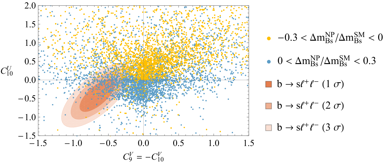
Note that the contributions in Eqs. (19, 21), which would require the addition of the four Fermion operators in Eq. (17) are all proportional to $\varepsilon^{d}$ , which we set to zero in our analysis. Finally, semi-leptonic decays are important to constrain vector operators since their dependence on scalar ones is very weak Becirevic:2012fy. However, many processes and observables have been measured and one therefore should use a global fit to constrain $C_{9,10}^{(\prime)\mu\mu}$ (taking also into account $B_{s}\to\mu^{+}\mu^{-}$ if one assumes the absence of scalar operators). The scenario with a lepton flavour conserving $C_{10}$ effect ( $C_{10}^{U}$ ) and a contribution to $C_{9}=-C_{10}$ with muons only ( $C_{9}^{V}=-C_{10}^{V}$ ) (following the conventions of Ref. Alguero:2018nvb) is phenomenologically the most important scenario for us. We will discuss this in the next section.

Concerning the case of decays into tau leptons, one can calculate the semi-leptonic processes using the relevant expressions for the factors. We use the results of Ref. Capdevila:2017iqn and find for tau leptons

\displaystyle\begin{split}10^{7}\times{\rm{Br}}&\left[{{B}\to K\tau^{+}\tau^{-}}\right]^{[15,22]}=\Big(1.20+0.15\,C_{9}^{\prime}-0.42\,C_{10}^{\prime}+0.02\,C_{9}^{\prime\,2}\\ &+0.05\,C_{10}^{\prime\,2}+0.15\,C_{9}^{\text{NP}}-0.42\,C_{10}^{\text{NP}}+0.04\,C_{9}^{\text{NP}}C_{9}^{\prime}+0.10\,C_{10}^{\text{NP}}C_{10}^{\prime}\\ &+0.02\,C_{9}^{\text{NP}\,2}+0.05\,C_{10}^{\text{NP}\,2}\Big)\pm\Big(0.12+0.02\,C_{9}^{\text{NP}}-0.04\,C_{10}^{\text{NP}}\\ &+0.01\,C_{9}^{\prime}-0.04\,C_{10}^{\prime}+0.08\,C_{10}^{\prime\,2}+0.01\,C_{10}^{\text{NP}}C_{10}^{\prime}+0.01\,C_{10}^{\text{NP}\,2}\Big)\,,\\ \end{split}

(51)

\displaystyle\begin{split}10^{7}\times{\rm{Br}}&\left[{{B}\to K^{*}\tau^{+}\tau^{-}}\right]^{[15,19]}=\Big(0.98-0.30\,C_{9}^{\prime}+0.12\,C_{10}^{\prime}+0.05\,C_{9}^{\prime\,2}\\ &+0.02\,C_{10}^{\prime\,2}+0.38\,C_{9}^{\text{NP}}-0.14\,C_{10}^{\text{NP}}-0.08\,C_{9}^{\text{NP}}C_{9}^{\prime}-0.03\,C_{10}^{\text{NP}}C_{10}^{\prime}\\ &+0.05\,C_{9}^{\text{NP}\,2}+0.02\,C_{10}^{\text{NP}\,2}\Big)\pm\Big(0.09+0.03\,C_{9}^{\text{NP}}-0.01\,C_{10}^{\text{NP}}\\ &-0.01\,C_{9}^{\text{NP}}C_{9}^{\prime}-0.03\,C_{9}^{\prime}-0.01\,C_{9}^{\prime}C_{10}^{\prime}+0.01\,C_{9}^{\prime\,2}-0.01\,C_{10}^{\prime\,2}\Big)\,,\end{split}

(52)

\displaystyle\begin{split}10^{7}\times&{\rm{Br}}\left[{B_{s}}\to\phi\tau^{+}\tau^{-}\right]^{[15,18.8]}=\Big(0.86-0.28\,C_{9}^{\prime}+0.10\,C_{10}^{\prime}+0.05\,C_{9}^{\prime\,2}\\ &+0.01\,C_{10}^{\prime\,2}+0.34\,C_{9}^{\text{NP}}-0.11\,C_{10}^{\text{NP}}-0.08\,C_{9}^{\text{NP}}C_{9}^{\prime}-0.02\,C_{10}^{\text{NP}}C_{10}^{\prime}\\ &+0.05\,C_{9}^{\text{NP}\,2}+0.01\,C_{10}^{\text{NP}\,2}\Big)\pm\big(0.06+0.02\,C_{9}^{\text{NP}}-0.02\,C_{9}^{\prime}+0.02\,C_{10}^{\prime\,2}\big)\,.\end{split}

(53)

For lepton flavour violating transitions one finds Crivellin:2015era

\displaystyle\text{Br}[B\to K\ell^{+}\ell^{\prime-}]

\displaystyle=10^{-9}\left(a_{K\ell\ell^{\prime}}\left|C_{9}^{\ell\ell^{\prime}}+C_{9}^{\prime\ell\ell^{\prime}}\right|^{2}+b_{K\ell\ell^{\prime}}\left|C_{10}^{\ell\ell^{\prime}}+C_{10}^{\prime\ell\ell^{\prime}}\right|^{2}\right)\,,

(54)

\displaystyle\begin{split}\text{Br}[B\to K^{*}\ell^{+}\ell^{\prime-}]&=10^{-9}\left(a_{K^{*}\ell\ell^{\prime}}\left|C_{9}^{\ell\ell^{\prime}}+C_{9}^{\prime\ell\ell^{\prime}}\right|^{2}+b_{K^{*}\ell\ell^{\prime}}\left|C_{10}^{\ell\ell^{\prime}}+C_{10}^{\prime\ell\ell^{\prime}}\right|^{2}\right.\\ &~~+\left.c_{K^{*}\ell\ell^{\prime}}\left|C_{9}^{\ell\ell^{\prime}}-C_{9}^{\prime\ell\ell^{\prime}}\right|^{2}+d_{K^{*}\ell\ell^{\prime}}\left|C_{10}^{\ell\ell^{\prime}}-C_{10}^{\prime\ell\ell^{\prime}}\right|^{2}\right)\,,\end{split}

(55)

with

$\ell\ell^{\prime}$	$a_{K\ell\ell^{\prime}}$	$b_{K\ell\ell^{\prime}}$	$a_{K^{*}\ell\ell^{\prime}}$	$b_{K^{*}\ell\ell^{\prime}}$	$c_{K^{*}\ell\ell^{\prime}}$	$d_{K^{*}\ell\ell^{\prime}}$
$\;\tau\mu\;$	$\;9.6\pm 1.0\;$	$\;10.0\pm 1.3\;$	$\;3.0\pm 0.8\;$	$\;2.7\pm 0.7\;$	$\;16.4\pm 2.1\;$	$\;15.4\pm 1.9\;$
$\mu e$	$15.4\pm 3.1$	$15.7\pm 3.1$	$5.6\pm 1.9$	$5.6\pm 1.9$	$29.1\pm 4.9$	$29.1\pm 4.9$

4 $b\to s\nu\bar{\nu}$ , $B_{s}-\bar{B}_{s}$ Mixing, $a_{\mu}$ and $\ell\to\ell^{\prime}\gamma$

Let us now turn to the matching for the remaining $b\to s$ processes, $b\to s\nu\bar{\nu}$ and $B_{s}-\bar{B}_{s}$ mixing. In addition, we consider the anomalous magnetic moments of charged leptons together with the closely related radiative lepton decays and $h\to\tau\mu$ .

4.1 $b\to s\nu\bar{\nu}$

For $b\to s\nu\bar{\nu}$ processes the corresponding effective Hamiltonian is defined as

\displaystyle H_{eff}^{{\nu_{I}}{\nu_{J}}}

\displaystyle=

\displaystyle-\dfrac{{4{G_{F}}}}{{\sqrt{2}}}{V_{tb}}V_{ts}^{*}\left({C_{L}^{IJ}O_{L}^{IJ}+C_{R}^{IJ}O_{R}^{IJ}}\right)\,,

(56)

with the operators

\displaystyle O_{L}^{IJ}

\displaystyle=\dfrac{{{e^{2}}}}{{16{\pi^{2}}}}\bar{s}{\gamma_{\mu}}{P_{L}}b{{\bar{\nu}}_{I}}{\gamma^{\mu}}\left({1-{\gamma_{5}}}\right){\nu_{J}}\,,

\displaystyle O_{R}^{IJ}

\displaystyle=\dfrac{{{e^{2}}}}{{16{\pi^{2}}}}\bar{s}{\gamma_{\mu}}{P_{R}}b{{\bar{\nu}}_{I}}{\gamma^{\mu}}\left({1-{\gamma_{5}}}\right){\nu_{J}}\,.

(57)

From box diagrams with charged Higgses we obtain

	$\displaystyle C_{L}^{IJ}$	$\displaystyle=\frac{y}{g_{2}^{4}s_{W}^{2}V_{tb}V_{ts}^{}}\big(V_{m2}^{}\varepsilon_{mi}^{u}\varepsilon_{li}^{u}{V_{l3}}U_{nI}^{}\varepsilon_{nj}^{\ell}\varepsilon_{pj}^{\ell*}{U_{pJ}}\big)I_{1}(z_{i})\,,$		(58)
	$\displaystyle C_{R}^{IJ}$	$\displaystyle=\frac{y}{g_{2}^{4}s_{W}^{2}V_{tb}V_{ts}^{}}\big(\varepsilon_{m2}^{d}V_{im}^{}{V_{il}}\varepsilon_{l3}^{d}U_{nI}^{}\varepsilon_{nj}^{\ell}\varepsilon_{pj}^{\ell*}{U_{pJ}}\big)I_{1}(z_{i})\,.$		(59)

We follow Buras:2014fpa and define

\epsilon_{IJ}=\frac{\sqrt{\big|C_{L}^{IJ}\big|^{2}+\big|C_{R}^{IJ}\big|^{2}}}{\big|C_{L}^{SM}\big|},\qquad\eta_{IJ}=\frac{-{\rm Re}\left[C_{L}^{IJ}C_{R}^{JI*}\right]}{\big|C_{L}^{IJ}\big|^{2}+\big|C_{R}^{IJ}\big|^{2}}\,.

(60)

This allows us to write the branching ratio in terms of

R_{K}=\frac{1}{3}\sum_{\{I,J\}=1}^{3}(1-2\eta_{IJ})\epsilon_{IJ}^{2},\qquad R_{K^{*}}=\frac{1}{3}\sum_{\{I,J\}=1}^{3}(1+\kappa_{\eta}\eta_{IJ})\epsilon_{IJ}^{2}\,,

(61)

where $\kappa_{\eta}$ encapsules the dependence on the form factors. In Ref. Buras:2014fpa this quantity is evaluated using as input for the $B\to K^{*}$ form factors a combined fit to lattice and LCSR results performed in Straub:2015ica, finding $\kappa_{\eta}=1.34\pm 0.04$ . The branching ratio reads

\mathrm{Br}\left[B\to X_{s}\nu\bar{\nu}\right]\approx\mathrm{Br}\left[B\to X_{s}\nu\bar{\nu}\right]_{\rm{SM}}\left(\frac{\kappa_{\eta}R_{K}+2R_{K}^{*}}{2+\kappa_{\eta}}\right)\,.

(62)

This has to be compared to the experimental limits Grygier:2017tzo

{R_{K}^{\nu\bar{\nu}}}<3.9\,,\qquad{R_{{K^{*}}}^{\nu\bar{\nu}}}<2.7\,.

(63)

4.2 $B_{s}-\bar{B}_{s}$ Mixing

The effective Hamiltonian is defined as

\displaystyle H_{\rm eff}^{\Delta F=2}=\sum_{a=1}^{5}C_{a}O_{a}+\sum_{a=1}^{3}C_{a}^{\prime}O_{a}^{\prime}\,,

(64)

with

\displaystyle\begin{aligned} O_{1}^{(\prime)}&=\left[\bar{s}_{\alpha}\gamma^{\mu}P_{L(R)}b_{\alpha}\right]\left[\bar{s}_{\beta}\gamma_{\mu}P_{L(R)}b_{\beta}\right]\,,&&&O_{2}^{(\prime)}&=\left[\bar{s}_{\alpha}P_{L(R)}b_{\alpha}\right]\left[\bar{s}_{\beta}P_{L(R)}b_{\beta}\right]\,,\\ O_{3}^{(\prime)}&=\left[\bar{s}_{\alpha}P_{L(R)}b_{\beta}\right]\left[\bar{s}_{\beta}P_{L(R)}b_{\alpha}\right]\,,&&&O_{4}&=\left[\bar{s}_{\alpha}P_{L}b_{\alpha}\right]\left[\bar{s}_{\beta}P_{R}b_{\beta}\right]\,,\\ O_{5}&=\left[\bar{s}_{\alpha}P_{L}b_{\beta}\right]\left[\bar{s}_{\beta}P_{R}b_{\alpha}\right]\,.\end{aligned}

(65)

We obtain at tree level (see left diagram in Fig. 7)

\displaystyle\begin{split}C_{2}&=-\frac{1}{2}\big(\varepsilon_{32}^{d*}\big)^{2}\bigg(\frac{s_{\beta\alpha}^{2}}{m_{H_{0}}^{2}}+\frac{c_{\beta\alpha}^{2}}{m_{h_{0}}^{2}}-\frac{1}{m_{A_{0}}^{2}}\bigg)\,,\\ C_{2}^{\prime}&=-\frac{1}{2}\big(\varepsilon_{23}^{d}\big)^{2}\bigg(\frac{s_{\beta\alpha}^{2}}{m_{H_{0}}^{2}}+\frac{c_{\beta\alpha}^{2}}{m_{h_{0}}^{2}}-\frac{1}{m_{A_{0}}^{2}}\bigg)\,,\\ C_{4}&=-\varepsilon_{23}^{d}\varepsilon_{32}^{d*}\bigg(\frac{s_{\beta\alpha}^{2}}{m_{H_{0}}^{2}}+\frac{c_{\beta\alpha}^{2}}{m_{h_{0}}^{2}}+\frac{1}{m_{A_{0}}^{2}}\bigg)\,.\end{split}

(66)

\begin{overpic}[tree-level.pdf] \put(12.0,33.0){\footnotesize$b$} \put(12.0,3.0){\footnotesize$s$} \put(36.0,23.0){\footnotesize$H^{0},h^{0},A^{0}$} \put(81.0,33.0){\footnotesize$s$} \put(81.0,3.0){\footnotesize$b$} \end{overpic}

\begin{overpic}[box_HH.pdf] \put(10.0,41.0){\footnotesize$b$} \put(10.0,4.0){\footnotesize$s$} \put(30.0,25.0){\footnotesize$c,t$} \put(61.0,25.0){\footnotesize$c,t$} \put(47.0,41.0){\footnotesize$H^{-}$} \put(47.0,4.0){\footnotesize$H^{-}$} \put(88.0,4.0){\footnotesize$b$} \put(88.0,41.0){\footnotesize$s$} \end{overpic}

\begin{overpic}[box_HW.pdf] \put(10.0,41.0){\footnotesize$b$} \put(10.0,4.0){\footnotesize$s$} \put(30.0,25.0){\footnotesize$c,t$} \put(61.0,25.0){\footnotesize$c,t$} \put(47.0,40.0){\footnotesize$W^{-}$} \put(47.0,4.0){\footnotesize$H^{-}$} \put(88.0,4.0){\footnotesize$b$} \put(88.0,41.0){\footnotesize$s$} \end{overpic}

Figure 7: Feynman diagrams contributing to

B_{s}-\bar{B}_{s}

mixing. Note that the tree-level contribution is absent for

\varepsilon_{23}^{d}=\varepsilon_{32}^{d}=0

Like in the case for $b\to s\ell^{+}\ell^{-}$ , we only calculate a loop effect in the case of a vanishing tree-level contribution, i.e. for $\varepsilon^{d}_{23,32}=0$ . In agreement with Ref. Crivellin:2013wna we find for the pure $H^{+}$ boxes

\displaystyle\begin{split}C_{1}&=-\frac{\big(V_{k2}^{*}\varepsilon_{kj}^{u}\varepsilon_{lj}^{u*}V_{l3}\big)\big(V_{m2}^{*}\varepsilon_{mi}^{u}\varepsilon_{ni}^{u*}V_{n3}\big)}{32\pi^{2}m_{H^{+}}^{2}}I_{8}(z_{j},z_{i})\,,\\ C_{1}^{\prime}&=-\frac{\big(\varepsilon^{d*}_{22}\varepsilon^{d}_{33}V^{*}_{i2}V_{i3}\big)\big(\varepsilon^{d*}_{22}\varepsilon^{d}_{33}V^{*}_{j2}V_{j3}\big)}{32\pi^{2}m_{H^{+}}^{2}}I_{9}(z_{i},z_{j})\,,\\ C_{2}&=-\frac{\big(\varepsilon_{22}^{d*}V_{j2}^{*}\varepsilon_{lj}^{u*}V_{l3}\big)\big(\varepsilon_{22}^{d*}V_{i2}^{*}\varepsilon_{ni}^{u*}V_{n3}\big)}{8\pi^{2}}\frac{\sqrt{z_{i}}\sqrt{z_{j}}}{m_{H^{+}}^{2}}I_{10}(z_{i},z_{j})\,,\\ C_{2}^{\prime}&=-\frac{\big(V^{*}_{n2}\varepsilon^{u}_{ni}V_{i3}\varepsilon^{d}_{33}\big)\big(V^{*}_{l2}\varepsilon^{u}_{lj}V_{j3}\varepsilon^{d}_{33}\big)}{8\pi^{2}}\frac{\sqrt{z_{i}}\sqrt{z_{j}}}{m_{H^{+}}^{2}}I_{10}(z_{i},z_{j})\,,\\ C_{4}&=-\frac{\big(\varepsilon_{22}^{d*}V_{j2}^{*}\varepsilon_{lj}^{u*}V_{l3}\big)\big(V_{m2}^{*}\varepsilon_{mi}^{u}V_{i3}\varepsilon_{33}^{d}\big)}{4\pi^{2}}\frac{\sqrt{z_{i}}\sqrt{z_{j}}}{m_{H^{+}}^{2}}I_{10}(z_{i},z_{j})\,,\\ C_{5}&=\frac{\big(\varepsilon_{22}^{d*}V_{j2}^{*}V_{j3}\varepsilon_{33}^{d}\big)\big(V_{m2}^{*}\varepsilon_{mk}^{u}\varepsilon_{nk}^{u*}V_{n3}\big)}{8\pi^{2}m_{H^{+}}^{2}}\left(I_{8}(z_{j},z_{k})+I_{1}(z_{j})\right)\,,\end{split}

(67)

and for the $W^{+}$ - $H^{+}$ boxes

\displaystyle\begin{split}C_{1}&=\frac{g_{2}^{2}}{64\pi^{2}}\frac{\sqrt{z_{j}}\sqrt{z_{k}}}{m_{W}^{2}}\big(V_{j2}^{*}\varepsilon_{ij}^{u*}V_{i3}\big)\big(V_{l2}^{*}\varepsilon_{lk}^{u}V_{k3}\big)I_{11}(y,z_{k},z_{j})\,,\\ C_{4}&=-\frac{g_{2}^{2}\big(\varepsilon^{d*}_{22}\varepsilon^{d}_{33}V^{*}_{k2}V_{k3}V^{*}_{j2}V_{j3}\big)}{16\pi^{2}m_{W}^{2}}I_{12}(z_{j},z_{k})\,.\end{split}

(68)

The corresponding diagrams are shown in Fig. 7. The loop functions are given in the appendix and once more we did not distinguish between the cases of light and heavy quarks, since the contribution of the light quarks trivially follows by taking the convergent limit $z_{i}\to 0$ .

Phenomenologically, we only need to consider the contributions to $C_{1}$ , since the other Wilson coefficients are proportional to $\varepsilon^{d}_{ij}$ which we will assume to be small. The constraints on NP crucially depend on the hadronic matrix elements calculated in lattice QCD. While Ref. DiLuzio:2017fdq finds a preference for destructive interference with the SM, Ref. Bona:2007vi finds a preference for constructive interference. We will therefore use the ratio $C_{1}^{\rm NP}/C_{1}^{\rm SM}$ , where all hadronic uncertainties drop out. We assume a conservative bound of $\pm 30\%$ .

4.3 $\ell\to\ell^{\prime}\gamma$ and $a_{\ell}$

Since it is important for our phenomenological analysis, we generalize the formula of Ref. Crivellin:2013wna to include right-handed neutrinos. Following the conventions of Ref. Crivellin:2018qmi we define

\displaystyle\mathcal{H}_{\rm eff}=c_{R}^{\ell_{F}\ell_{I}}\bar{\ell}_{F}\sigma_{\mu\nu}P_{R}\ell_{I}F^{\mu\nu}+{\rm h.c.}\,,

(69)

with

\displaystyle a_{\ell_{I}}=-\frac{4m_{\ell_{I}}}{e}\Re\left[c_{R}^{\ell_{I}\ell_{I}}\right]\,,

(70)

and

\displaystyle{\rm Br}\left[\ell_{I}\to\ell_{F}\gamma\right]=\frac{m_{\ell_{I}}^{3}}{4\pi}\tau_{\ell_{I}}\left(\big|c_{R}^{FI}\big|^{2}+\big|c_{R}^{IF}\big|^{2}\right)\,.

(71)

For the loop diagrams with charged Higgses we obtain

\displaystyle\begin{split}c_{R}^{\ell_{F}\ell_{I}}&=-\frac{em_{\ell_{I}}\big(U_{Fk}\varepsilon_{kj}^{\nu}\varepsilon_{nj}^{\nu*}U_{In}^{*}\big)}{192\pi^{2}m_{H^{+}}^{2}}\bigg[\frac{2x_{j}^{2}+5x_{j}-1}{(1-x_{j})^{3}}+\frac{6x_{j}^{2}\log(x_{j})}{(1-x_{j})^{4}}\bigg]+\frac{em_{\ell_{F}}\varepsilon_{kF}^{\ell*}\varepsilon_{kI}^{\ell}}{192\pi^{2}m_{H^{+}}^{2}}\,,\\ c_{L}^{\ell_{F}\ell_{I}}&=-\frac{em_{\ell_{F}}\big(U_{Fk}\varepsilon_{kj}^{\nu}\varepsilon_{nj}^{\nu*}U_{In}^{*}\big)}{192\pi^{2}m_{H^{+}}^{2}}\bigg[\frac{2x_{j}^{2}+5x_{j}-1}{(1-x_{j})^{3}}+\frac{6x_{j}^{2}\log(x_{j})}{(1-x_{j})^{4}}\bigg]+\frac{em_{\ell_{I}}\varepsilon_{kF}^{\ell*}\varepsilon_{kI}^{\ell}}{192\pi^{2}m_{H^{+}}^{2}}\,,\end{split}

(72)

where we set the left-handed neutrino mass to zero. The neutral Higgs bosons give

\displaystyle\begin{split}c_{R}^{\ell_{F}\ell_{I}}&=\!\!\!\!\!\!\!\sum_{H=\{H_{0},h_{0},A_{0}\}}\!\!\!\!\!\!\!\!-\frac{e\left(m_{\ell_{F}}\Gamma_{jF}^{H*}\Gamma_{jI}^{H}+m_{\ell_{I}}\Gamma_{jF}^{H*}\Gamma_{jI}^{H}\right)}{192\pi^{2}m_{H}^{2}}\!+\!\frac{e\,m_{\ell_{j}}\Gamma_{Fj}^{H}\Gamma_{jI}^{H}}{64\pi^{2}m_{H}^{2}}\Bigg(\!3+2\log\!\bigg(\frac{m_{\ell_{j}}^{2}}{m_{H}^{2}}\bigg)\!\Bigg)\end{split}

(73)

with

\displaystyle\Gamma_{FI}^{H_{0}}

\displaystyle=c_{\beta\alpha}\frac{m_{\ell_{F}}}{v}\delta_{FI}-s_{\beta\alpha}\varepsilon^{\ell}_{FI}\,,

\displaystyle\Gamma_{FI}^{h_{0}}

\displaystyle=s_{\beta\alpha}\frac{m_{\ell_{F}}}{v}\delta_{FI}+c_{\beta\alpha}\varepsilon^{\ell}_{FI}\,,

\displaystyle\Gamma_{FI}^{A_{0}}

\displaystyle=i\varepsilon_{FI}^{\ell}\,.

(74)

Also here, we included the hard matching contribution together with the soft contribution from the effective theory in the formula since we do not aim at calculating QED corrections Crivellin:2017rmk. For our purposes we require only the lepton flavour violating decay $\tau\to\mu\gamma$ whose experimental upper limit is given by $\mathrm{Br}\left[\tau\to\mu\gamma\right]<4.4\cdot 10^{-8}$ Aubert:2009ag; Hayasaka:2007vc.

4.4 $h\to\tau\mu$

Here, we find for the decay width

\displaystyle\Gamma\left[h\to\tau\mu\right]\simeq\frac{3c_{\beta\alpha}^{2}m_{h}}{8\pi}\Big(|\varepsilon_{23}^{\ell}|^{2}+|\varepsilon_{32}^{\ell}|^{2}\Big)\left(1-\frac{m_{\tau}^{2}}{m_{h}^{2}}\right)^{2}\,,

(75)

with $\Gamma_{\mathrm{SM}}\simeq 4.1{\rm MeV}$ . This has to be compared to the current experimental limit Aad:2016blu; Khachatryan:2015kon

\displaystyle{\rm Br}\left[h\to\tau\mu\right]\leq 1.43\%\,.

(76)

Due to the suppressed SM decay width, $h\to\tau\mu$ will turn out to be surprisingly constraining.

Figure 8: Effect in

B_{s}-\bar{B}_{s}

mixing and

C_{10}^{U}

in the

\varepsilon^{u}_{23}

\varepsilon^{u}_{32}

plane for

M_{H^{+}}=400\mathrm{GeV}

assuming all other couplings

\varepsilon=0

. Note that the relative effect in

C_{10}^{U}

with respect to the one in

B_{s}-\bar{B}_{s}

mixing is to a good approximation independent of the Higgs masses. The small allowed regions in the bottom-left (top-right) of the plot correspond to cancellations between boxes with two charged Higgses and mixed boxes with

W

and

H^{\pm}

5 Phenomenological Analysis

In our numerical analysis we want to focus on the possibility to explain the hints for NP in $b\to s\mu^{+}\mu^{-}$ transitions and $a_{\mu}$ within 2HDMs. Concerning $b\to s\mu^{+}\mu^{-}$ data, it is well-known from global fits that a sizeable contribution to the Wilson coefficient $C_{9}$ (and possibly also $C_{10}$ ) is required to explain the data. Additional substantial effects in $C_{9}^{\prime}$ and $C_{10}^{\prime}$ are possible. However, contributions to scalar operators must be suppressed due to the strong constraints from $B_{s}\to\mu^{+}\mu^{-}$ where they enter with an enhancement factor of $m_{b}^{2}/m_{\mu}^{2}$ .

Figure 9: Prediction for the decay of the SM-like Higgs boson

h\to\tau\mu

as a function of

\varepsilon^{\ell}_{32}

under the assumption that

\varepsilon^{\ell}_{23}

is chosen in such a way that the anomalous magnetic moment of the muon is explained. We used

M_{H^{+}}=400\mathrm{GeV}

M_{H_{0}}=250\mathrm{GeV}

and

M_{A_{0}}=300\mathrm{GeV}

. For

c_{\beta\alpha}=0.003

the whole

2\,\sigma

region to explain

a_{\mu}

is shown while for

c_{\beta\alpha}=0.001

and

c_{\beta\alpha}=0.005

only the predictions for the central value of

a_{\mu}

are depicted.

$C_{9}$ and $C_{10}$ can only be generated from $\gamma$ and $Z$ penguins (see Eqs. (38)-(40)) or from charged Higgs boxes (see Eq. (45)). Interestingly, all contributions to $C_{9}$ and $C_{10}$ involve $\varepsilon^{u}_{ij}$ but not $\varepsilon^{d}_{ij}$ while the effect in $C_{9}^{\prime}$ , $C_{10}^{\prime}$ only appears once $\varepsilon^{d}_{ii}$ is unequal to zero. Furthermore, scalar operators involve both $\varepsilon^{d}_{ii}$ and $\varepsilon^{u}_{ij}$ . To accommodate the strong constraints on scalar operators we will assume that $\varepsilon^{d}_{ii}$ is negligibly small in the following. As stated above, an effect in $C_{9}$ is mandatory to explain the anomalies. However, the $Z$ penguin contribution to $C_{9}$ is suppressed by $(1-4s_{W}^{2})$ and the off-shell photon effect is small due to the electromagnetic coupling. Hence, in the limit of $\varepsilon^{\ell}_{ij}=\varepsilon^{\nu}_{ij}=0$ we are left with a lepton flavour universal $C_{10}^{U}$ effect (following the conventions of Ref. Alguero:2018nvb) to a good approximation. This effect is also strongly correlated to (and therefore limited by) $B_{s}-\bar{B}_{s}$ mixing, as shown in Fig. 8. Note that this correlation is to a good approximation independent of the Higgs masses. The bound from $b\to s\gamma$ in this setup turns out to be in general weaker than the ones from $B_{s}-\bar{B}_{s}$ mixing.

Therefore, we need in addition the charged Higgs boxes if we aim at a good fit to $b\to s\mu^{+}\mu^{-}$ data. Here, $\varepsilon^{\ell}_{I2}$ generates $C_{9}^{V}=C_{10}^{V}$ effect in muons only, while $\varepsilon_{2I}^{\nu}$ gives $C_{9}^{V}=-C_{10}^{V}$ . Let us first consider the case with only $\varepsilon^{\ell}_{IJ}$ since these couplings are present also in the scenario without right-handed neutrinos. Since we aim at an explanation of $a_{\mu}$ , we focus on the elements $\varepsilon^{\ell}_{23,32}$ which give an $m_{\tau}/m_{\mu}$ enhanced effect in this observable⁵⁵ 5 Since it is a chirally enhanced effect, it has a free phase and can thus give a sizeable effect in the electric dipole moment of the muon Crivellin:2018qmi.. For the numerical analysis we chose for definiteness $m_{A_{0}}=300\,$ GeV and $m_{H_{0}}=250\,$ GeV. Even though a detailed collider analysis is well beyond the scope of this article, note that the small values of $c_{\beta\alpha}$ are compatible with direct LHC searches Sirunyan:2018koj. The effect in $a_{\mu}$ is directly correlated to $h\to\tau\mu$ which strongly constrains $c_{\beta\alpha}$ as shown in Fig. 9. The bounds from $h\to\tau\mu$ do not only depend on fewer parameters than $\tau\to\mu\gamma$ but are even much stronger for $\varepsilon_{22,33}^{\ell}=0$ . Concerning $b\to s\ell^{+}\ell^{-}$ , the impact with $\varepsilon^{\ell}_{23,32}\neq 0$ is small. Since the effect in $a_{\mu}$ is chirally enhanced, it significantly limits the product $\varepsilon^{\ell}_{23}\varepsilon^{\ell}_{32}$ rendering the deviation from $C_{9}^{V}=-C_{10}^{V}$ unimportant.

In a next step, we allow for the presence of right-handed neutrinos and $\varepsilon_{ij}^{\nu}\neq 0$ where the $C_{9}^{V}=-C_{10}^{V}$ effect has to be added to $C_{10}^{U}$ from the $Z$ penguin. The result is shown in Fig. 10 where we can see that it is difficult to find points which give a good fit to $b\to s\mu^{+}\mu^{-}$ data. While the effect of $\varepsilon_{IJ}^{\nu}\neq 0$ in $a_{\mu}$ is always destructive, i.e. it increases the discrepancy between theory and experiment, the effect is small since it is not enhanced by $m_{\tau}/m_{\mu}$ . It is therefore possible to tackle $b\to s\mu^{+}\mu^{-}$ fixing $\varepsilon^{\nu}_{IJ}$ and $\delta a_{\mu}$ fixing $\varepsilon^{\ell}_{IJ}$ semi independently, while choosing the Higgs masses consistent with direct searches and taking into account the smallness of $c_{\beta\alpha}$ , required by $h\to\tau\mu$ . One can see that in order to be in agreement with $b\to s\ell^{+}\ell^{-}$ data, positive effects in $B_{s}-\bar{B}_{s}$ mixing are preferred.

Refer to caption — Figure 10: Scatter plot with $\varepsilon^{u}_{22,32,23,33}$ and $\varepsilon^{\nu}_{21,22,32,23,33}$ varied between $\pm 1.5$ . Concerning the masses we scanned over are (in GeV) $m_{N_{i}}\in[100,1000]$ , $m_{H^{+}}\in[100,500]$ and $\{m_{H_{0}},m_{A_{0}}\}\in[100,350]$ . In total, we generated $10^{6}$ points. The red regions are preferred by $b\to s\ell^{+}\ell^{-}$ data according to updated fit of Ref. Alguero:2019ptt and includes the new LHCb Aaij:2019wad and Belle BelleMoriond measurement of $R(K)$ and $R(K^{*})$ , respectively. It is interesting to note that using the new fit significantly more points lie within the preferred regions.

6 Conclusions

In this article we studied $b\to s$ transitions in 2HDMs with generic Yukawa couplings (including right-handed neutrinos) with focus on $b\to s\mu^{+}\mu^{-}$ transitions and its possible correlations with $a_{\mu}$ . We first recalled the tree-level effects in $b\to s$ observables which involve $\varepsilon^{d}_{23,32}$ . If these elements are zero or negligibly small, loop effects involving $W$ bosons and charged Higgses can become numerically important. We calculated these leading one-loop corrections to $b\to s\ell^{+}\ell^{-}$ , $b\to s\nu\bar{\nu}$ and $\Delta B=\Delta S=2$ transitions in a general $R_{\xi}$ gauge and confirmed their correctness finding gauge invariant results. Additionally, we discuss the treatment of self-energy contributions and renormalization in detail. In addition, we provided the formula for $\tau\to\mu\gamma$ and $a_{\mu}$ including the contributions from heavy (TeV scale) right-handed neutrinos.

Concerning the phenomenology, we found that without right-handed neutrinos sizeable contributions to vector operators can only be generated via photon and $Z$ penguins. However, this does not allow for lepton flavour universality violation and the effect in $C_{10}^{U}$ with respect to $C_{9}^{U}$ is too big to give a good fit to data. Therefore, we included in a next step right-handed neutrinos which lead in general to a lepton flavour universality violating $C_{9}^{V}=-C_{10}^{V}$ effect. This can provide an explanation of the anomalies especially with the recently updated $b\to s\ell^{+}\ell^{-}$ data.

If we allow for Higgs to $\tau\mu$ couplings, we can explain the anomalous magnetic moment by a chirally enhanced $m_{\tau}/m_{\mu}$ effect. This leads at the same time to non-vanishing branching ratios $\tau\to\mu\gamma$ and $\tau\to 3\mu$ which are however compatible with the experimental limits. The effect in $h\to\tau\mu$ is found to be dominant, i.e. most constraining. In case of an explanation of $a_{\mu}$ , $h\to\tau\mu$ requires a close alignment in the Higgs sector, i.e. very small $c_{\beta\alpha}$ . Furthermore, a small $C_{9}^{V}=+C_{10}^{V}$ effect is generated which does not significantly improve the goodness of the fit to data.

2HDMs have a rich flavour phenomenology since they give effects in many classes of observables. As we showed in this article, these models are in principle capable to explain the discrepancies between the SM and experiment. Once one allows for a generic flavour structure and right-handed neutrinos, this provides a possible solution to the deviations in $b\to s\ell^{+}\ell^{-}$ transitions and $a_{\mu}$ , even though some degree of finetuning is necessary. Furthermore, also the anomalies in $b\to c\tau\nu$ processes Amhis:2016xyh might be addressed by 2HDMs Crivellin:2012ye; Crivellin:2013wna; Celis:2012dk; Ko:2012sv; Crivellin:2015hha; Dhargyal:2016eri; Chen:2017eby; Iguro:2017ysu; Martinez:2018ynq; Biswas:2018jun. However, these solutions are under pressure from the measurement of the $B_{c}$ lifetime Celis:2016azn; Alonso:2016oyd; Akeroyd:2017mhr; Blanke:2018yud and LHC searches Faroughy:2016osc. Furthermore, also the $\epsilon^{\prime}/\epsilon$ anomaly (see e.g. Ref. Aebischer:2018csl for a review) could be explained Chen:2018vog; Marzo:2019ldg, leaving 2HDMs still as one of the most appealing NP scenarios.

Acknowledgments

The work of A.C. and D.M. is supported by an Ambizione Grant (PZ00P2_154834) and a Professorship Grant (PP00P2_176884) of the Swiss National Science Foundation. The work of C.W. is supported by the Swiss National Foundation under grant 200020_175449/1. We are grateful to Bernat Capdevilla for providing us with the global fit used for Fig. 10 and to Emanuele Bagnaschi for useful discussions. We thank Christoph Greub for collaboration in the early stages of the project and for useful comments on the manuscript.

Appendix

We define the Higgs potential as

\displaystyle\begin{split}\mathcal{V}(\Phi_{1},\Phi_{2})&=m_{11}^{2}\Phi_{1}^{\dagger}\Phi_{1}+m_{22}^{2}\Phi_{2}^{\dagger}\Phi_{2}-\big(m_{12}^{2}\Phi_{1}^{\dagger}\Phi_{2}+m_{12}^{2*}\Phi_{2}^{\dagger}\Phi_{1}\big)+\frac{\lambda_{1}}{2}\big(\Phi_{1}^{\dagger}\Phi_{1}\big)^{2}\\ &~~+\frac{\lambda_{2}}{2}\big(\Phi_{2}^{\dagger}\Phi_{2}\big)^{2}+\lambda_{3}\big(\Phi_{1}^{\dagger}\Phi_{1}\big)\big(\Phi_{2}^{\dagger}\Phi_{2}\big)+\lambda_{4}\big(\Phi_{1}^{\dagger}\Phi_{2}\big)\big(\Phi_{2}^{\dagger}\Phi_{1}\big)\\ &~~+\frac{\lambda_{5}}{2}\Big(\big(\Phi_{1}^{\dagger}\Phi_{2}\big)^{2}+\big(\Phi_{2}^{\dagger}\Phi_{1}\big)^{2}\Big)\,.\end{split}

(77)

Using the definition of Eq. (4) and transforming to the CP-even mass eigenstates according to Eq. (5), we express $m_{11}$ , $m_{22}$ , $m_{21}$ , $\lambda_{1}$ and $\lambda_{4}$ in terms of the Higgs masses. Therefore, the remaining couplings are $\lambda_{2}$ , $\lambda_{3}$ and $\lambda_{5}$ . The triple Higgs couplings appearing in Eq. (42) are then given by

\displaystyle\begin{split}\lambda_{h_{0}H^{+}H^{-}}&=vs_{\beta\alpha}\lambda_{3}\,,\\ \lambda_{H_{0}H^{+}H^{-}}&=vc_{\beta\alpha}\lambda_{3}\,.\end{split}

(78)

Note that with these conventions the expressions are as simple as possible and only $\lambda_{3}$ enters.

Loop Functions

The loop functions that we used throughout our article are defined as

\displaystyle\begin{aligned} f_{1}(b)&=\dfrac{{\left({12{b}\left({\log\left({b}\right)-1}\right)-3b^{2}\left({6\log\left(b\right)+1}\right)+8b^{3}+7}\right)}}{{{{\left({1-b}\right)}^{4}}}}\,,\\ f_{2}(b)&=\dfrac{{\left({{4\log\left(b\right)+3}-2b\left({3\log\left(b\right)+4}\right)+5b^{2}}\right)}}{{{{\left({1-b}\right)}^{3}}}}\,,\\ f_{3}(b)&=\dfrac{{\left({3{b}\left({2\log\left(b\right)+1}\right)-6b^{2}+b^{3}+2}\right)}}{{{{\left({1-{b}}\right)}^{4}}}}\,,\\ f_{4}(b)&=\dfrac{{\left({{2\log\left(b\right)+3}-4{b}+b^{2}}\right)}}{{{{\left({1-{b}}\right)}^{3}}}}\,,\\ f_{5}(b)&=\dfrac{{2\left({12\log\left(b\right)+19}\right)-9{b}\left({4\log\left(b\right)+13}\right)}}{{{{\left({1-{b}}\right)}^{4}}}}+\dfrac{126b^{2}+b^{3}\left({18\log\left(b\right)-47}\right)}{{{{\left({1-{b}}\right)}^{4}}}}\,,\\ I_{0}\left(b\right)&=\dfrac{1-3b}{-1+b}+\dfrac{2b^{2}\log\left(b\right)}{\left(b-1\right)^{2}}\,,\\ I_{1}\left(b\right)&=-\dfrac{1}{b-1}+\dfrac{\log\left(b\right)b}{\left(b-1\right)^{2}}\,,\\ I_{2}\left(b\right)&=\dfrac{\log\left(b\right)b}{1-b}=(1-b)I_{1}(b)-1\,,\\ I_{3}\left(a,b\right)&=\dfrac{(7a-b)b}{a-b}+\dfrac{2b^{2}\log\left(b\right)(2a^{2}-b^{2}-6a+3b+2ab)}{\left(a-b\right)^{2}(b-1)}-\dfrac{6a^{2}b\log\left(a\right)}{\left(a-b\right)^{2}}\,,\\ I_{4}\left(a,b\right)&=\dfrac{\sqrt{a^{3}}\sqrt{b}\log\left(a\right)}{(a-1)(a-b)}-\dfrac{\sqrt{a}\sqrt{b^{3}}\log\left(b\right)}{(b-1)(a-b)},\\ I_{5}\left(a,b\right)&=-1+\dfrac{a^{2}\log\left(a\right)}{(a-1)(a-b)}-\dfrac{b^{2}\log\left(b\right)}{(b-1)(a-b)},\\ I_{6}\left(b\right)&=-b+\dfrac{b^{2}\log\left(b\right)}{b-1}=b(b-1)I_{1}(b),\\ I_{7}\left(b\right)&=\dfrac{b}{b-1}-\dfrac{b^{2}\log\left(b\right)}{\left(b-1\right)^{2}}=-bI_{1}(b)\,\\ I_{8}(a,b)&=\frac{-1}{(1-a)(1-b)}+\frac{b^{2}\log(b)}{(1-b)^{2}(a-b)}+\frac{a^{2}\log(a)}{(1-a)^{2}(b-a)}\,,\\ I_{9}(a,b)&=\frac{-ab}{(1-a)(1-b)}+\frac{ab\log(b)}{(1-b)^{2}(a-b)}+\frac{ab\log(a)}{(1-a)^{2}(b-a)}\,,\\ I_{10}(a,b)&=\frac{-1}{(1-a)(1-b)}+\frac{a\log(a)}{(1-a)^{2}(b-a)}+\frac{b\log(b)}{(1-b)^{2}(a-b)}\,,\\ I_{11}(a,b,c)&=\frac{-3a^{2}\log(a)}{(a-1)(a-b)(a-c)}+\frac{b(4a-b)\log(b)}{(b-1)(a-b)(b-c)}+\frac{c(4a-c)\log(c)}{(c-1)(a-c)(c-b)}\,,\\ I_{12}(a,b)&=\frac{ab\log(a)}{(1-a)(a-b)}-\frac{ab\log(b)}{(1-b)(a-b)}\,.\end{aligned}

(79)

If the Higgs penguins contain a charm quark in the loop (whose mass we neglect), i.e. $z_{2}=0$ , the loop functions simplify to

\displaystyle\begin{aligned} I_{0}(0)&=-1\,,\\ I_{1}(0)&=1\,,\\ I_{4}(b,0)&=I_{4}(0,b)=I_{4}(0,0)=0\,,\\ I_{5}(b,0)&=I_{5}(0,b)=-1+\frac{b\log(b)}{b-1}\,,\\ I_{5}(0,0)&=-1\,,\\ I_{7}(0)&=0\,,\\ I_{8}(0,x_{j})&=I_{1}(x_{j})\,,\end{aligned}

(80)

and the corresponding Wilsons coefficients in Eq. (42) become

\displaystyle\begin{split}C_{S(HH)}^{IJ}=&\dfrac{-y\varepsilon^{d*}_{22}L_{+}^{IJ}}{2g_{2}^{4}s_{W}^{2}V^{*}_{ts}V_{tb}}\Big[4t_{2}\big(\varepsilon^{d}_{33}V^{*}_{k2}\varepsilon^{u}_{k2}V_{23}-\varepsilon^{d*}_{33}V^{*}_{22}\varepsilon^{u*}_{n2}V_{n3}\big)+V^{*}_{k2}\varepsilon^{u}_{k2}\varepsilon^{u*}_{n2}V_{n3}\\ &-2\log\left(\dfrac{\mu^{2}}{m_{H^{+}}^{2}}\right)\Big(2\left(\varepsilon^{d}_{33}V^{*}_{k2}\varepsilon^{u}_{k2}V_{23}-\varepsilon^{d*}_{33}V^{*}_{22}\varepsilon^{u*}_{n2}V_{n3}\right)t_{2}\\ &+V_{n3}(2V^{*}_{22}\varepsilon^{u*}_{n2}\varepsilon^{u}_{22}+2V^{*}_{22}\varepsilon^{u*}_{n3}\varepsilon^{u}_{23}+2V^{*}_{32}\varepsilon^{u*}_{n2}\varepsilon^{u}_{32}-V^{*}_{k2}\varepsilon^{u*}_{n2}\varepsilon^{u}_{k2})\Big)\\ &-4\left(V^{*}_{22}\varepsilon^{u}_{22}\varepsilon^{u*}_{n2}V_{n3}-I_{5}\left(z_{3},0\right)\left(V^{*}_{22}\varepsilon^{u}_{23}\varepsilon^{u*}_{n3}V_{n3}+V^{*}_{32}\varepsilon^{u}_{32}\varepsilon^{u*}_{n2}V_{n3}\right)\right)\Big]\end{split}

(81)

\displaystyle\begin{split}C_{S(HH)}^{\prime IJ}\!=&\dfrac{yL_{-}^{IJ}}{g_{2}^{4}s_{W}^{2}V^{*}_{ts}V_{tb}}\!\!\Big[\!-\!2t_{2}\big(\!\left(\varepsilon^{d}_{33}\right)^{\!2}V^{*}_{k2}\varepsilon^{u}_{k2}V_{23}\!-\!\varepsilon^{d*}_{22}\varepsilon^{d}_{22}V^{*}_{22}\varepsilon^{u*}_{n2}V_{n3}\big)\\ &+\!2\log\left(\dfrac{\mu^{2}}{m_{H^{+}}^{2}}\!\right)\!\Big(\!\!-\!\varepsilon^{d}_{33}V^{*}_{k2}\varepsilon^{u}_{k2}\varepsilon^{u*}_{22}V_{23}-\!\varepsilon^{d}_{33}V^{*}_{k2}\varepsilon^{u}_{k2}\varepsilon^{u*}_{32}V_{33}-\!\varepsilon^{d}_{33}V^{*}_{k2}\varepsilon^{u}_{k3}\varepsilon^{u*}_{23}V_{23}\!\\ &+\!\left(\!\left(\varepsilon^{d}_{33}\right)^{\!2}\!V^{*}_{k2}\varepsilon^{u}_{k2}V_{23}\!-\!\varepsilon^{d*}_{22}\varepsilon^{d}_{22}V^{*}_{22}\varepsilon^{u*}_{n2}V_{n3}\!\right)\!t_{2}\Big)-2\varepsilon^{d}_{33}V^{*}_{k2}\varepsilon^{u}_{k2}\varepsilon^{u*}_{22}V_{23}\\ &+\varepsilon^{d}_{33}\big(-\varepsilon^{d*}_{22}\varepsilon^{d}_{22}V^{*}_{22}V_{23}+2I_{5}\left(z_{3},0\right)V^{*}_{k2}\left(\varepsilon^{u}_{k3}\varepsilon^{u*}_{23}V_{23}+\varepsilon^{u}_{k2}\varepsilon^{u*}_{32}V_{33}\right)\big)\Big]\end{split}

(82)

References

(1) T. D. Lee, A Theory of Spontaneous T Violation, Phys. Rev. D8 (1973) 1226.
(2) J. F. Gunion, H. E. Haber, G. L. Kane and S. Dawson, The Higgs Hunter’s Guide, Front. Phys. 80 (2000) 1.
(3) G. C. Branco, P. M. Ferreira, L. Lavoura, M. N. Rebelo, M. Sher and J. P. Silva, Theory and phenomenology of two-Higgs-doublet models, Phys. Rept. 516 (2012) 1 [1106.0034].
(4) J. E. Kim, Light Pseudoscalars, Particle Physics and Cosmology, Phys. Rept. 150 (1987) 1.
(5) R. D. Peccei and H. R. Quinn, CP Conservation in the Presence of Instantons, Phys. Rev. Lett. 38 (1977) 1440.
(6) M. Trodden, Electroweak baryogenesis: A Brief review, in Proceedings, 33rd Rencontres de Moriond 98 electrowek interactions and unified theories: Les Arcs, France, Mar 14-21, 1998, pp. 471–480, 1998, hep-ph/9805252.
(7) H. E. Haber and G. L. Kane, The Search for Supersymmetry: Probing Physics Beyond the Standard Model, Phys. Rept. 117 (1985) 75.
(8) A. Crivellin, M. Ghezzi and M. Procura, Effective Field Theory with Two Higgs Doublets, JHEP 09 (2016) 160 [1608.00975].
(9) D. Bhatia, U. Maitra and S. Niyogi, Discovery prospects of a light Higgs boson at the LHC in type-I 2HDM, Phys. Rev. D97 (2018) 055027 [1704.07850].
(10) A. Arbey, F. Mahmoudi, O. Stal and T. Stefaniak, Status of the Charged Higgs Boson in Two Higgs Doublet Models, Eur. Phys. J. C78 (2018) 182 [1706.07414].
(11) P. Basler, P. M. Ferreira, M. Mühlleitner and R. Santos, High scale impact in alignment and decoupling in two-Higgs doublet models, Phys. Rev. D97 (2018) 095024 [1710.10410].
(12) U. Haisch and A. Malinauskas, Let there be light from a second light Higgs doublet, JHEP 03 (2018) 135 [1712.06599].
(13) L. Jenniches, C. Sturm and S. Uccirati, Electroweak corrections in the 2HDM for neutral scalar Higgs-boson production through gluon fusion, JHEP 09 (2018) 017 [1805.05869].
(14) N. Chen, C. Du, Y. Wu and X.-J. Xu, Further study of the global minimum constraint on the two-Higgs-doublet models: LHC searches for heavy Higgs bosons, Phys. Rev. D99 (2019) 035011 [1810.04689].
(15) R. Enberg, W. Klemm, S. Moretti and S. Munir, Electroweak production of multiple (pseudo)scalars in the 2HDM, 1812.01147.
(16) A. Arhrib, R. Benbrik, H. Harouiz, S. Moretti and A. Rouchad, A Guidebook to Hunting Charged Higgs Bosons at the LHC, 1810.09106.
(17) E. Hanson, W. Klemm, R. Naranjo, Y. Peters and A. Pilaftsis, Charged Higgs Bosons in Naturally Aligned Two Higgs Doublet Models at the LHC, 1812.04713.
(18) X. G. He, T. D. Nguyen and R. R. Volkas, $B$ Meson Rare Decays in Two Higgs Doublets Models, Phys. Rev. D38 (1988) 814.
(19) W. Skiba and J. Kalinowski, $B_{s}\to\tau^{+}\tau^{-}$ decay in a two Higgs doublet model, Nucl. Phys. B404 (1993) 3.
(20) Y.-B. Dai, C.-S. Huang and H.-W. Huang, $B\to X(s)\tau^{+}\tau^{-}$ in a two Higgs doublet model, Phys. Lett. B390 (1997) 257 [hep-ph/9607389].
(21) C.-S. Huang and Q.-S. Yan, $B\to X_{s}\tau^{+}\tau^{-}$ in the flipped SU(5) model, Phys. Lett. B442 (1998) 209 [hep-ph/9803366].
(22) H. E. Logan and U. Nierste, $B_{s,d}\to\ell^{+}\ell^{-}$ in a two Higgs doublet model, Nucl. Phys. B586 (2000) 39 [hep-ph/0004139].
(23) X.-D. Cheng, Y.-D. Yang and X.-B. Yuan, Revisiting $B_{s}\to\mu^{+}\mu^{-}$ in the two-Higgs doublet models with $Z_{2}$ symmetry, Eur. Phys. J. C76 (2016) 151 [1511.01829].
(24) P. Arnan, D. Bečirević, F. Mescia and O. Sumensari, Two Higgs doublet models and $b\rightarrow s$ exclusive decays, Eur. Phys. J. C77 (2017) 796 [1703.03426].
(25) E. O. Iltan and G. Turan, $B_{S}\to\tau^{+}\tau^{-}$ decay in the general two Higgs doublet model, JHEP 11 (2002) 031 [hep-ph/0011005].
(26) X.-Q. Li, J. Lu and A. Pich, $B_{s,d}^{0}\to\ell^{+}\ell^{-}$ Decays in the Aligned Two-Higgs-Doublet Model, JHEP 06 (2014) 022 [1404.5865].
(27) F. Mahmoudi and O. Stal, Flavor constraints on the two-Higgs-doublet model with general Yukawa couplings, Phys. Rev. D81 (2010) 035016 [0907.1791].
(28) A. J. Buras, M. V. Carlucci, S. Gori and G. Isidori, Higgs-mediated FCNCs: Natural Flavour Conservation vs. Minimal Flavour Violation, JHEP 10 (2010) 009 [1005.5310].
(29) A. Crivellin, A. Kokulu and C. Greub, Flavor-phenomenology of two-Higgs-doublet models with generic Yukawa structure, Phys. Rev. D87 (2013) 094031 [1303.5877].
(30) A. Crivellin, J. Heeck and D. Müller, Large $h\to bs$ in generic two-Higgs-doublet models, Phys. Rev. D97 (2018) 035008 [1710.04663].
(31) HFLAV collaboration, Averages of $b$ -hadron, $c$ -hadron, and $\tau$ -lepton properties as of summer 2016, Eur. Phys. J. C77 (2017) 895 [1612.07233].
(32) CMS, LHCb collaboration, Observation of the rare $B^{0}_{s}\to\mu^{+}\mu^{-}$ decay from the combined analysis of CMS and LHCb data, Nature 522 (2015) 68 [1411.4413].
(33) LHCb collaboration, Measurement of the $B^{0}_{s}\to\mu^{+}\mu^{-}$ branching fraction and search for $B^{0}\to\mu^{+}\mu^{-}$ decays at the LHCb experiment, Phys. Rev. Lett. 111 (2013) 101805 [1307.5024].
(34) CMS collaboration, Measurement of the $B^{0}_{s}\to\mu^{+}\mu^{-}$ Branching Fraction and Search for $B^{0}\to\mu^{+}\mu^{-}$ with the CMS Experiment, Phys. Rev. Lett. 111 (2013) 101804 [1307.5025].
(35) ATLAS collaboration, Study of the rare decays of $B^{0}_{s}$ and $B^{0}$ mesons into muon pairs using data collected during 2015 and 2016 with the ATLAS detector, Submitted to: JHEP (2018) [1812.03017].
(36) C. Bobeth, M. Gorbahn, T. Hermann, M. Misiak, E. Stamou and M. Steinhauser, $B_{s,d}\to l^{+}l^{-}$ in the Standard Model with Reduced Theoretical Uncertainty, Phys. Rev. Lett. 112 (2014) 101801 [1311.0903].
(37) M. Beneke, C. Bobeth and R. Szafron, Enhanced electromagnetic correction to the rare $B$ -meson decay $B_{s,d}\to\mu^{+}\mu^{-}$ , Phys. Rev. Lett. 120 (2018) 011801 [1708.09152].
(38) B. Capdevila, A. Crivellin, S. Descotes-Genon, J. Matias and J. Virto, Patterns of New Physics in $b\to s\ell^{+}\ell^{-}$ transitions in the light of recent data, JHEP 01 (2018) 093 [1704.05340].
(39) M. Alguero, B. Capdevila, A. Crivellin, S. Descotes-Genon, P. Masjuan, J. Matias et al., Addendum: ”Patterns of New Physics in $b\to s\ell^{+}\ell^{-}$ transitions in the light of recent data”, 1903.09578.
(40) W. Altmannshofer, P. Stangl and D. M. Straub, Interpreting Hints for Lepton Flavor Universality Violation, Phys. Rev. D96 (2017) 055008 [1704.05435].
(41) G. D’Amico, M. Nardecchia, P. Panci, F. Sannino, A. Strumia, R. Torre et al., Flavour anomalies after the $R_{K^{*}}$ measurement, JHEP 09 (2017) 010 [1704.05438].
(42) L.-S. Geng, B. Grinstein, S. Jäger, J. Martin Camalich, X.-L. Ren and R.-X. Shi, Towards the discovery of new physics with lepton-universality ratios of $b\to s\ell\ell$ decays, Phys. Rev. D96 (2017) 093006 [1704.05446].
(43) M. Ciuchini, A. M. Coutinho, M. Fedele, E. Franco, A. Paul, L. Silvestrini et al., On Flavourful Easter eggs for New Physics hunger and Lepton Flavour Universality violation, Eur. Phys. J. C77 (2017) 688 [1704.05447].
(44) G. Hiller and I. Nisandzic, $R_{K}$ and $R_{K^{\ast}}$ beyond the standard model, Phys. Rev. D96 (2017) 035003 [1704.05444].
(45) T. Hurth, F. Mahmoudi, D. Martinez Santos and S. Neshatpour, Lepton nonuniversality in exclusive $b{\rightarrow}s{\ell}{\ell}$ decays, Phys. Rev. D96 (2017) 095034 [1705.06274].
(46) M. Ciuchini, A. M. Coutinho, M. Fedele, E. Franco, A. Paul, L. Silvestrini et al., New Physics in $b\to s\ell^{+}\ell^{-}$ confronts new data on Lepton Universality, 1903.09632.
(47) M. Misiak et al., Updated NNLO QCD predictions for the weak radiative B-meson decays, Phys. Rev. Lett. 114 (2015) 221801 [1503.01789].
(48) Belle collaboration, Search for $B\to h\nu\bar{\nu}$ decays with semileptonic tagging at Belle, Phys. Rev. D96 (2017) 091101 [1702.03224].
(49) BaBar collaboration, Search for $B\to K^{(*)}\nu\overline{\nu}$ and invisible quarkonium decays, Phys. Rev. D87 (2013) 112005 [1303.7465].
(50) A. J. Buras, J. Girrbach-Noe, C. Niehoff and D. M. Straub, $B\to{K}^{\left(\ast\right)}\nu\overline{\nu}$ decays in the Standard Model and beyond, JHEP 02 (2015) 184 [1409.4557].
(51) S.-P. Li, X.-Q. Li, Y.-D. Yang and X. Zhang, ${R}_{D^{\left(*\right)}},{R}_{K^{\left(*\right)}}$ and neutrino mass in the 2HDM-III with right-handed neutrinos, JHEP 09 (2018) 149 [1807.08530].
(52) C. Marzo, L. Marzola and M. Raidal, Common explanation to the $R_{K^{(*)}}$ , $R_{D^{(*)}}$ and $\epsilon^{\prime}/\epsilon$ anomalies in a 3HDM+ $\nu_{R}$ and connections to neutrino physics, 1901.08290.
(53) Muon g-2 collaboration, Final Report of the Muon E821 Anomalous Magnetic Moment Measurement at BNL, Phys. Rev. D73 (2006) 072003 [hep-ex/0602035].
(54) Muon g-2 collaboration, Muon (g-2) Technical Design Report, 1501.06858.
(55) J-PARC g-’2/EDM collaboration, A novel precision measurement of muon g-2 and EDM at J-PARC, AIP Conf. Proc. 1467 (2012) 45.
(56) T. P. Gorringe and D. W. Hertzog, Precision Muon Physics, Prog. Part. Nucl. Phys. 84 (2015) 73 [1506.01465].
(57) A. Czarnecki, B. Krause and W. J. Marciano, Electroweak Fermion loop contributions to the muon anomalous magnetic moment, Phys. Rev. D52 (1995) R2619 [hep-ph/9506256].
(58) A. Czarnecki, B. Krause and W. J. Marciano, Electroweak corrections to the muon anomalous magnetic moment, Phys. Rev. Lett. 76 (1996) 3267 [hep-ph/9512369].
(59) C. Gnendiger, D. Stöckinger and H. Stöckinger-Kim, The electroweak contributions to $(g-2)_{\mu}$ after the Higgs boson mass measurement, Phys. Rev. D88 (2013) 053005 [1306.5546].
(60) T. Aoyama, T. Kinoshita and M. Nio, Revised and Improved Value of the QED Tenth-Order Electron Anomalous Magnetic Moment, Phys. Rev. D97 (2018) 036001 [1712.06060].
(61) M. Della Morte, A. Francis, V. Gülpers, G. Herdoíza, G. von Hippel, H. Horch et al., The hadronic vacuum polarization contribution to the muon $g-2$ from lattice QCD, JHEP 10 (2017) 020 [1705.01775].
(62) M. Davier, A. Hoecker, B. Malaescu and Z. Zhang, Reevaluation of the hadronic vacuum polarisation contributions to the Standard Model predictions of the muon $g-2$ and ${\alpha(m_{Z}^{2})}$ using newest hadronic cross-section data, Eur. Phys. J. C77 (2017) 827 [1706.09436].
(63) Budapest-Marseille-Wuppertal collaboration, Hadronic vacuum polarization contribution to the anomalous magnetic moments of leptons from first principles, Phys. Rev. Lett. 121 (2018) 022002 [1711.04980].
(64) RBC, UKQCD collaboration, Calculation of the hadronic vacuum polarization contribution to the muon anomalous magnetic moment, Phys. Rev. Lett. 121 (2018) 022003 [1801.07224].
(65) A. Keshavarzi, D. Nomura and T. Teubner, Muon $g-2$ and $\alpha(M_{Z}^{2})$ : a new data-based analysis, Phys. Rev. D97 (2018) 114025 [1802.02995].
(66) D. Giusti, F. Sanfilippo and S. Simula, Light-quark contribution to the leading hadronic vacuum polarization term of the muon $g-2$ from twisted-mass fermions, Phys. Rev. D98 (2018) 114504 [1808.00887].
(67) G. Colangelo, M. Hoferichter and P. Stoffer, Two-pion contribution to hadronic vacuum polarization, JHEP 02 (2019) 006 [1810.00007].
(68) A. Gérardin, H. B. Meyer and A. Nyffeler, Lattice calculation of the pion transition form factor $\pi^{0}\to\gamma^{*}\gamma^{*}$ , Phys. Rev. D94 (2016) 074507 [1607.08174].
(69) T. Blum, N. Christ, M. Hayakawa, T. Izubuchi, L. Jin, C. Jung et al., Connected and Leading Disconnected Hadronic Light-by-Light Contribution to the Muon Anomalous Magnetic Moment with a Physical Pion Mass, Phys. Rev. Lett. 118 (2017) 022005 [1610.04603].
(70) G. Colangelo, M. Hoferichter, M. Procura and P. Stoffer, Rescattering effects in the hadronic-light-by-light contribution to the anomalous magnetic moment of the muon, Phys. Rev. Lett. 118 (2017) 232001 [1701.06554].
(71) G. Colangelo, M. Hoferichter, M. Procura and P. Stoffer, Dispersion relation for hadronic light-by-light scattering: two-pion contributions, JHEP 04 (2017) 161 [1702.07347].
(72) T. Blum, N. Christ, M. Hayakawa, T. Izubuchi, L. Jin, C. Jung et al., Using infinite volume, continuum QED and lattice QCD for the hadronic light-by-light contribution to the muon anomalous magnetic moment, Phys. Rev. D96 (2017) 034515 [1705.01067].
(73) M. Hoferichter, B.-L. Hoid, B. Kubis, S. Leupold and S. P. Schneider, Pion-pole contribution to hadronic light-by-light scattering in the anomalous magnetic moment of the muon, Phys. Rev. Lett. 121 (2018) 112002 [1805.01471].
(74) A. Kurz, T. Liu, P. Marquard and M. Steinhauser, Hadronic contribution to the muon anomalous magnetic moment to next-to-next-to-leading order, Phys. Lett. B734 (2014) 144 [1403.6400].
(75) G. Colangelo, M. Hoferichter, A. Nyffeler, M. Passera and P. Stoffer, Remarks on higher-order hadronic corrections to the muon g-2, Phys. Lett. B735 (2014) 90 [1403.7512].
(76) H. Georgi and D. V. Nanopoulos, Suppression of Flavor Changing Effects From Neutral Spinless Meson Exchange in Gauge Theories, Phys. Lett. 82B (1979) 95.
(77) L. Lavoura and J. P. Silva, Fundamental CP violating quantities in a SU(2) x U(1) model with many Higgs doublets, Phys. Rev. D50 (1994) 4619 [hep-ph/9404276].
(78) F. J. Botella and J. P. Silva, Jarlskog - like invariants for theories with scalars and fermions, Phys. Rev. D51 (1995) 3870 [hep-ph/9411288].
(79) S. Davidson, $\mu\rightarrow e\gamma$ in the 2HDM: an exercise in EFT, Eur. Phys. J. C76 (2016) 258 [1601.01949].
(80) CMS collaboration, Combined measurements of Higgs boson couplings in proton-proton collisions at $\sqrt{s}=$ 13 TeV, Submitted to: Eur. Phys. J. (2018) [1809.10733].
(81) ATLAS collaboration, Combined measurements of Higgs boson production and decay using up to 80 fb^-1 of proton–proton collision data at $\sqrt{s}=$ 13 TeV collected with the ATLAS experiment, .
(82) F. Borzumati and C. Greub, 2HDMs predictions for $\bar{B}\to X(s)\gamma$ in NLO QCD, Phys. Rev. D58 (1998) 074004 [hep-ph/9802391].
(83) F. Borzumati and C. Greub, Two Higgs doublet model predictions for $\bar{B}\to X(s)\gamma$ in NLO QCD: Addendum, Phys. Rev. D59 (1999) 057501 [hep-ph/9809438].
(84) A. Crivellin, Effective Higgs Vertices in the generic MSSM, Phys. Rev. D83 (2011) 056001 [1012.4840].
(85) A. J. Buras, P. H. Chankowski, J. Rosiek and L. Slawianowska, $\Delta M_{d,s},B^{0}_{d,s}\to\mu^{+}\mu^{-}$ and $B\to X_{s}\gamma$ in supersymmetry at large $\tan\beta$ , Nucl. Phys. B659 (2003) 3 [hep-ph/0210145].
(86) A. Crivellin and J. Girrbach, Constraining the MSSM sfermion mass matrices with light fermion masses, Phys. Rev. D81 (2010) 076001 [1002.0227].
(87) A. Dedes, J. Rosiek and P. Tanedo, Complete One-Loop MSSM Predictions for $B\to$ lepton lepton’ at the Tevatron and LHC, Phys. Rev. D79 (2009) 055006 [0812.4320].
(88) M. Misiak, A. Rehman and M. Steinhauser, NNLO QCD counterterm contributions to $\bar{B}\to X_{s\gamma}$ for the physical value of $m_{c}$ , Phys. Lett. B770 (2017) 431 [1702.07674].
(89) T. Hurth, E. Lunghi and W. Porod, Untagged $\bar{B}\to X_{s+d}\gamma$ CP asymmetry as a probe for new physics, Nucl. Phys. B704 (2005) 56 [hep-ph/0312260].
(90) D. Becirevic, N. Kosnik, F. Mescia and E. Schneider, Complementarity of the constraints on New Physics from $B_{s}\to\mu^{+}\mu^{-}$ and from $B\to Kl^{+}l^{-}$ decays, Phys. Rev. D86 (2012) 034034 [1205.5811].
(91) M. Algueró, B. Capdevila, S. Descotes-Genon, P. Masjuan and J. Matias, Are we overlooking Lepton Flavour Universal New Physics in $b\to s\ell\ell$ ?, 1809.08447.
(92) B. Capdevila, A. Crivellin, S. Descotes-Genon, L. Hofer and J. Matias, Searching for New Physics with $b\to s\tau^{+}\tau^{-}$ processes, Phys. Rev. Lett. 120 (2018) 181802 [1712.01919].
(93) A. Crivellin, L. Hofer, J. Matias, U. Nierste, S. Pokorski and J. Rosiek, Lepton-flavour violating $B$ decays in generic $Z^{\prime}$ models, Phys. Rev. D92 (2015) 054013 [1504.07928].
(94) A. Bharucha, D. M. Straub and R. Zwicky, $B\to V\ell^{+}\ell^{-}$ in the Standard Model from light-cone sum rules, JHEP 08 (2016) 098 [1503.05534].
(95) L. Di Luzio, M. Kirk and A. Lenz, Updated $B_{s}$ -mixing constraints on new physics models for $b\to s\ell^{+}\ell^{-}$ anomalies, Phys. Rev. D97 (2018) 095035 [1712.06572].
(96) UTfit online update collaboration, Model-independent constraints on $\Delta F=2$ operators and the scale of new physics, JHEP 03 (2008) 049 [0707.0636].
(97) A. Crivellin, M. Hoferichter and P. Schmidt-Wellenburg, Combined explanations of $(g-2)_{\mu,e}$ and implications for a large muon EDM, Phys. Rev. D98 (2018) 113002 [1807.11484].
(98) A. Crivellin, S. Davidson, G. M. Pruna and A. Signer, Renormalisation-group improved analysis of $\mu\to e$ processes in a systematic effective-field-theory approach, JHEP 05 (2017) 117 [1702.03020].
(99) BaBar collaboration, Searches for Lepton Flavor Violation in the Decays $\tau^{\pm}\to e^{\pm}\gamma$ and $\tau^{\pm}\to\mu^{\pm}\gamma$ , Phys. Rev. Lett. 104 (2010) 021802 [0908.2381].
(100) Belle collaboration, New Search for $\tau\to\mu\gamma$ and $\tau\to e\gamma$ Decays at Belle, Phys. Lett. B666 (2008) 16 [0705.0650].
(101) ATLAS collaboration, Search for lepton-flavour-violating decays of the Higgs and $Z$ bosons with the ATLAS detector, Eur. Phys. J. C77 (2017) 70 [1604.07730].
(102) CMS collaboration, Search for Lepton-Flavour-Violating Decays of the Higgs Boson, Phys. Lett. B749 (2015) 337 [1502.07400].
(103) LHCb collaboration, Search for lepton-universality violation in $B^{+}\to K^{+}\ell^{+}\ell^{-}$ decays, 1903.09252.
(104) M. Prim, Study of Lepton universality at Belle, Talk presented at Moriond EW on 22 ${\rm nd}$ of March 2019 .
(105) A. Crivellin, C. Greub and A. Kokulu, Explaining $B\to D\tau\nu$ , $B\to D^{*}\tau\nu$ and $B\to\tau\nu$ in a 2HDM of type III, Phys. Rev. D86 (2012) 054014 [1206.2634].
(106) A. Celis, M. Jung, X.-Q. Li and A. Pich, Sensitivity to charged scalars in $b\to d^{(*)}\tau\nu_{\tau}$ and $b\to\tau\nu_{\tau}$ decays, JHEP 01 (2013) 054 [1210.8443].
(107) P. Ko, Y. Omura and C. Yu, $B\to D^{(*)}\tau\nu$ and $B\to\tau\nu$ in chiral $U(1)^{\prime}$ models with flavored multi Higgs doublets, JHEP 03 (2013) 151 [1212.4607].
(108) A. Crivellin, J. Heeck and P. Stoffer, A perturbed lepton-specific two-Higgs-doublet model facing experimental hints for physics beyond the Standard Model, Phys. Rev. Lett. 116 (2016) 081801 [1507.07567].
(109) L. Dhargyal, $R(D^{(*)})$ and $Br(B\rightarrow\tau\nu_{\tau})$ in a Flipped/Lepton-Specific 2HDM with anomalously enhanced charged Higgs coupling to $\tau$ /b, Phys. Rev. D93 (2016) 115009 [1605.02794].
(110) C.-H. Chen and T. Nomura, Charged-Higgs on $R_{D^{(*)}}$ , $\tau$ polarization, and FBA, Eur. Phys. J. C77 (2017) 631 [1703.03646].
(111) S. Iguro and K. Tobe, $R(D^{(*)})$ in a general two Higgs doublet model, Nucl. Phys. B925 (2017) 560 [1708.06176].
(112) R. Martinez, C. F. Sierra and G. Valencia, Beyond $R(D^{(*)})$ with the general type-III 2HDM for $b\to c\tau\nu$ , Phys. Rev. D98 (2018) 115012 [1805.04098].
(113) A. Biswas, D. K. Ghosh, S. K. Patra and A. Shaw, $b\to c\ell\nu$ anomalies in light of extended scalar sectors, 1801.03375.
(114) A. Celis, M. Jung, X.-Q. Li and A. Pich, Scalar contributions to $b\to c(u)\tau\nu$ transitions, Phys. Lett. B771 (2017) 168 [1612.07757].
(115) R. Alonso, B. Grinstein and J. Martin Camalich, Lifetime of $B_{c}^{-}$ Constrains Explanations for Anomalies in $B\to D^{(*)}\tau\nu$ , Phys. Rev. Lett. 118 (2017) 081802 [1611.06676].
(116) A. G. Akeroyd and C.-H. Chen, Constraint on the branching ratio of $B_{c}\to\tau\bar{\nu}$ from LEP1 and consequences for $R(D^{(*)})$ anomaly, Phys. Rev. D96 (2017) 075011 [1708.04072].
(117) M. Blanke, A. Crivellin, S. de Boer, M. Moscati, U. Nierste, I. Nišandžić et al., Impact of polarization observables and $B_{c}\to\tau\nu$ on new physics explanations of the $b\to c\tau\nu$ anomaly, 1811.09603.
(118) D. A. Faroughy, A. Greljo and J. F. Kamenik, Confronting lepton flavor universality violation in B decays with high- $p_{T}$ tau lepton searches at LHC, Phys. Lett. B764 (2017) 126 [1609.07138].
(119) J. Aebischer, C. Bobeth, A. J. Buras and D. M. Straub, Anatomy of $\varepsilon^{\prime}/\varepsilon$ beyond the Standard Model, 1808.00466.
(120) C.-H. Chen and T. Nomura, $\epsilon^{\prime}/\epsilon$ from charged-Higgs-induced gluonic dipole operators, Phys. Lett. B787 (2018) 182 [1805.07522].

𝒃→𝒔​ℓ+​ℓ−b\to s\ell^{+}\ell^{-} Transitions in Two-Higgs-Doublet ModelsPreprint: PSI-PR-19-02, ZU-TH 10/19

Abstract

1 Introduction

2 Model and Conventions

3 𝒃→𝒔​ℓ+​ℓ−b\to s\ell^{+}\ell^{-} Processes

3.1 Tree-Level

3.2 𝒃→𝒔​𝜸b\to s\gamma

3.3 One-Loop Effects in 𝒃→𝒔ℓℓ(′)b\to s\ell\ell^{(\prime)}

3.3.1 Self-Energies and Renormalization

3.3.2 ZZ and γ\gamma Penguins

3.3.3 Higgs Penguin and WW-Higgs Boxes

3.3.4 H±H^{\pm} Boxes

3.4 Processes and Observables

4 𝒃→𝒔​𝝂​𝝂¯b\to s\nu\bar{\nu}, 𝑩𝒔−𝑩¯𝒔B_{s}-\bar{B}_{s} Mixing, 𝒂𝝁a_{\mu} and ℓ→ℓ′​𝜸\ell\to\ell^{\prime}\gamma

4.1 𝒃→𝒔​𝝂​𝝂¯b\to s\nu\bar{\nu}

4.2 Bs−B¯sB_{s}-\bar{B}_{s} Mixing

4.3 ℓ→ℓ′​𝜸\ell\to\ell^{\prime}\gamma and 𝒂ℓa_{\ell}

4.4 𝒉→𝝉​𝝁h\to\tau\mu

5 Phenomenological Analysis

6 Conclusions

Acknowledgments

Appendix

Loop Functions

References

$b\to s\ell^{+}\ell^{-}$ Transitions in Two-Higgs-Doublet ModelsPreprint: PSI-PR-19-02, ZU-TH 10/19

3 $b\to s\ell^{+}\ell^{-}$ Processes

3.2 $b\to s\gamma$

3.3 One-Loop Effects in $b\to s\ell\ell^{(\prime)}$

3.3.2 $Z$ and $\gamma$ Penguins

3.3.3 Higgs Penguin and $W$ -Higgs Boxes

3.3.4 $H^{\pm}$ Boxes

4 $b\to s\nu\bar{\nu}$ , $B_{s}-\bar{B}_{s}$ Mixing, $a_{\mu}$ and $\ell\to\ell^{\prime}\gamma$

4.1 $b\to s\nu\bar{\nu}$

4.2 $B_{s}-\bar{B}_{s}$ Mixing

4.3 $\ell\to\ell^{\prime}\gamma$ and $a_{\ell}$

4.4 $h\to\tau\mu$