Joint Active User Detection and Channel Estimation in Massive Access Systems Exploiting Reed-Muller Sequences
Abstract
The requirements to support massive connectivity and low latency in massive Machine Type Communications (mMTC) bring a huge challenge in the design of its random access (RA) procedure, which usually calls for efficient joint active user detection and channel estimation. In this paper, we exploit the vast sequence space and the beneficial nested structure of the length- second-order Reed-Muller (RM) sequences for designing an efficient RA scheme, which is capable of reliably detecting multiple active users from the set of unknown potential users with a size as large as , whilst simultaneously estimating their channel state information as well. Explicitly, at the transmitter each user is mapped to a specially designed RM sequence, which facilitates reliable joint sequence detection and channel estimation based on a single transmission event. To elaborate, as a first step, at the receiver we exploit the elegant nested structure of the RM sequences using a layer-by-layer RM detection algorithm for the single-user (single-sequence) scenario. Then an iterative RM detection and channel estimation algorithm is conceived for the multi-user (multi-sequence) scenario. As a benefit of the information exchange between the RM sequence detector and channel estimator, a compelling performance vs. complexity trade-off is struck, as evidenced both by our analytical and numerical results.
Index Terms:
mMTC, Massive access, Reed-Muller sequences, User identification, Channel estimation.I Introduction
I-A Motivation
The 5G wireless mobile network aims to support diverse applications, which were classified by 3GPP into three categories: enhanced Mobile Broadband (eMBB), Ultra-Reliable and Low Latency Communications (URLLC), and massive Machine Type Communications (mMTC)[1]. For the mMTC scenario, the key requirement is to provide massive connectivity for instant access of short and sporadic data traffic in applications like smart city and industrial internet of things [2].

The random access (RA) procedure is key to enable the massive connectivity. As depicted in Fig. 1 (a), in the current long term evolution (LTE) system, a four-message handshake between the user equipment (UE) and the access point (AP), which consists of Preamble, Random Access Response (RAR), Initial Layer 3 Message (Msg3) and Contention Resolution (CR) [3], is used for RA. If the UE successfully accesses the system, it completes the RA procedure by sending the “RRC Connection Setup Complete” message and starts to transmit its data. When applied to mMTC, this RA scheme faces two challenges. Firstly, the small-sized sequence space suffers from a high collision rate. When a UE triggers the RA procedure, it randomly chooses a preamble from the available sequence pool to send in the next RA slot. According to LTE [4], there are 54 Zadoff-Chu (ZC) sequences reserved for contention in each cell. If more than one UE select the same sequence, a collision occurs and these UEs must retransmit the sequence. In the context of massive connectivity, the frequent collisions and precipitated retransmissions will lead to network congestion, increased delay and resource wastage. Secondly, the traffic pattern exchanged in machine-type communications is typically short and sporadic [5]. A large amount of signalling will lead to high signalling-to-data ratio and low bandwidth efficiency. Since the ZC sequences do not carry any information about user identifiers (IDs) in the LTE system, the AP has no knowledge of exactly who is requiring access until Msg3 has been successfully received.
Hence, the preamble sequences play a vital role in the RA procedure. To satisfy the tight specifications of mMTC, the sequence space has to match the number of users in the system. Furthermore, predefined sequences with user IDs embedded in them are preferred for the sake of low signalling overhead and system latency. In this case, the AP has to detect the IDs of the active users and estimate the channel coefficients based on the received signal. To reduce congestion and achieve low latency, the above procedures have to be accomplished with high accuracy and at low complexity.
Moreover, it is worth pointing out that the difficulty of detecting active users from sets of potential users with different set sizes is very different. In general, detecting active users from a set of tens or hundreds of potential users can be readily achieved by elaborate sequence design and exhaustive search. However, it is rather challenging to do this in the massive access scenario where the number of unknown potential users can be as huge as hundreds of thousands or even millions, which makes the detection reminiscent of looking for the needle in a haystack.
I-B Related Work
Numerous researchers have improved the RA procedures by designing beneficial preamble sequences. Some of them focus on increasing the number of available ZC sequences. For example, the authors of [6] proposed a preamble reuse scheme by partitioning the cell coverage and reducing the cyclic shift size. Apart from the classic ZC sequences, [7] they inserted extra auxiliary sequences in the positions randomly chosen from the first data sub-frame. However, the use of auxiliary sequences decreases the data transmission efficiency and increases the detection complexity. By contrast, the RA procedure of [8] treats several RA slots as a virtual frame and the active users randomly choose a ZC sequence for their transmission in each slot. This is equivalent to expanding the sequence space at the cost of an increased overhead ratio and detection complexity.
Other authors investigate different sequence generation methods in support of massive connectivity and active user detection. On one hand, considering the huge number of potential users in the system, it is impossible to assign orthogonal sequences to each user. On the other hand, non-orthogonal sequences would inevitably impose multi-user interference during the detection. Hence, the key challenge is to obtain a relatively large sequence space, whilst simultaneously attaining reliable detection. Based on the sparsity of user-activity caused by the sporadic traffic in mMTC, the active user detection is often formulated as a compressive sensing (CS) problem. The active users transmit a unique sequence to access the system. To satisfy the so-called Restricted Isometry Property (RIP) of CS [9], the entries of these sequences are usually generated either by Gaussian or Bernoulli processes [10]. Hence, considerable storage resources are required for storing these sequences at the AP. At the receiver, CS algorithms, such as Basis Pursuit (BP) [11], Orthogonal Matching Pursuit (OMP) [12] and approximate message passing (AMP) [13][14], are utilized for detecting the active users. However, all these algorithms impose a high complexity that is related either to the size of sequence space or to the number of potential users in the system. Based on the code-expanded scheme of [8], the sequences constructed by Bloom filtering are utilized in [15]. Despite the lower latency compared to LTE, the hash functions used during the sequence generation have to be communicated both to all the users and to the AP, which imposes extra signalling overhead.
In [17], second-order RM sequences are invoked for massive access in 5G. Compared to ZC sequences, RM sequences have the following distinct advantages:
- •
The size of RM sequence space is several orders of magnitudes larger than that of the same-length ZC sequences, which meets the requirement of massive connectivity.
- •
The RM sequences can be uniquely and unambiguously mapped to user IDs. Hence, the AP can immediately infer the user ID right after the RM sequences have been correctly detected. Thus, the four-message handshake depicted in Fig. 1(a) is simplified to the twin-step interaction shown in Fig. 1(b), which results both in reduced signalling overhead and in reduced system latency.
- •
The structural properties of RM sequences can be exploited to design efficient detection algorithms having a low computational complexity.
In [16], RM sequences are used to construct the deterministic measurement matrix of CS, where an efficient reconstruction algorithm is also conceived, whose complexity is determined by the length of RM sequences and by the sparsity factor instead of the sequence space cardinality. However, this algorithm suffers from a serious performance degradation when the sparsity factor increases. Based on the algorithm in [16], a beneficial shuffle operation is advocated in [17] for improving the performance of RM detection, albeit at a high computational complexity. However, the compelling structural properties of RM sequences have not been fully exploited. In addition, to cope with the multi-sequence-induced interference, traditional successive interference cancellation (SIC) is adopted both in [16] and in [17], where the strongest signal is detected first and then subtracted from the received signal before detecting the next signal, regardless of whether the detected sequence is correct or not. Hence, once the sequence is incorrectly detected, it will affect the performance of all subsequent detection stages.
I-C Main Contributions
Considering the above attractive merits of RM sequences, we exploit them to facilitate active user detection and channel estimation in massive access systems in this paper. At the transmitter, each active user maps its ID to a unique RM sequence and then sends it to the AP. Here, a novel mapping rule is proposed. On one hand, it helps to improve the sequence detection performance. On the other hand, it enables us to accomplish sequence detection and channel estimation at the same time, without invoking an extra channel estimation step as the algorithms in [16] and [17].
At the receiver, we firstly design a single-sequence detection algorithm based on the nested structure of RM sequences, which reveals the relationships between its sub-sequences. Exploiting this structural property in the sequence detection algorithm, we intend to improve the detection performance at a reduced complexity. Moreover, to cope with the potential error propagation problem of the above algorithm, an enhanced algorithm based on multiple lists is also conceived. As for the case where multiple active users coexist in the system, an iterative RM detection and channel estimation algorithm is adopted. At each stage of an iteration, we focus on a particular user. Considering other signals as noise, the single-sequence detection algorithm is invoked for updating this user’s sequence detection result. After all the sequences are updated, the results are fed into the channel estimator to improve the accuracy of channel estimates. Then the enhanced channel estimates are utilized in the next iteration to reinforce the sequence detection.
Against the above background, our main contributions are:
- •
A novel mapping rule between user IDs and RM sequences is proposed, which helps to improve the sequence detection capability and simplify our high-accuracy channel estimation.
- •
We derive an explicit relationship between the RM sequence and its sub-sequences, which is referred to as nested structure. We exploit this structural property for conceiving a low-complexity algorithm for single sequence detection, which exhibits superior detection performance and channel estimation accuracy. In order to mitigate the error propagation, a moderate-complexity enhanced algorithm is also conceived.
- •
Iterative active-user detection and channel estimation scheme is then also proposed for the multi-sequence scenario. On one hand, the iterative detection may reduce the impact of incorrectly detected sequences. On the other hand, owing to the bi-directional information exchange between the active-user detector and channel estimator, the detection capability and channel estimation accuracy can mutually reinforce each other.
I-D Paper Organization and Notations
The rest of the paper is organized as follows. Section II describes the system model and introduces the transmitter and receiver structure of RA scheme using RM sequences. The nested structure of second-order RM sequences is derived in Section III. The blind active user detection and channel estimation algorithms are given in Section IV. Section V depicts the analytical model of the proposed algorithms and outlines the properties of them. Simulation Results are given in Section VI. And finally, Section VII concludes the paper.
Throughout this paper, scalars are represented in lower-case letters. Boldface lowercase and uppercase letters denote column vectors and matrices, respectively. and are column vectors of all zeros and all ones, respectively. We use to denote transpose of a matrix or vector and to denote complex conjugate. is the Euclidean norm. The symbol represents element-wise product and represents element-wise modulo-2 addition. indicates that is a complex Gaussian random variable with mean and variance . is reserved for complexity estimation.
II System Model
The massive uplink connectivity scenario illustrated in Fig. 2 is considered, where a single AP is serving a huge pool of users and the maximum value of depends on the sequence space size. All the users are assumed to be synchronized and each one of them has a unique user ID. In a specific RA slot, there are active users in the system and the active user set is denoted as . Due to the fact that the traffic pattern in mMTC scenario is typically sporadic, it is satisfied that .


The transmitter and receiver structure is shown in Fig. 3. To access the system, every active user will simultaneously send an RM sequence along with its ID to the AP in the next available RA slot. The AP has to accomplish both active user detection and channel estimation based on the received signal. In the sequel, the processes at the transmitter and the receiver are described in detail, respectively.
A length- second-order RM sequence is determined by an -element symmetric binary matrix and an -element binary vector . According to [16], given the matrix-vector pair , the -th entry of the RM sequence is expressed as
| (1) |
where is the imaginary unit that satisfies , denotes the Hamming weight of the vector , i.e., the number of s in , and is the -bit binary expression of .
To generate its RM sequence, the active user , first maps the user ID to the matrix-vector pair . We propose a novel mapping rule as follows:
- 1.
Convert the user ID to the length- binary vector .
- 2.
Put these bits successively into the symmetric matrix having zero diagonal elements, i.e.,
- 3.
The vector is constructed according to
(2)
Finally, the active user generates the RM sequence with the mapped matrix-vector pair . According to the above mapping rule, both the Hamming weight of the vector and the term must be even. With the normalization coefficient being omitted, the generation function shown in (1) can be simplified to
| (3) |
The size of the sequence space created by the proposed mapping rule is up to and the same-sized user space can be supported. In this sense, RM sequences are more suitable for massive access in mMTC scenario. Furthermore, the above mapping method also brings benefits for channel estimation and sequence detection, which will be specified in Section V.
All the active users in this RA slot simultaneously send their RM sequences to the AP and the received signal can be expressed as
| (4) |
where represents the channel coefficient between the active user and the AP, which is modeled as a complex Gaussian random process with unit variance, and is the complex additive white Gaussian noise (AWGN) having mean zero and variance . After receiving the signal, the AP has to detect all active users and estimate the corresponding channel coefficients. Thanks to the one-to-one mapping between the matrix-vector pair and the user ID, active user detection can be accomplished by recovering the matrix-vector pairs from the received signal.
III The nested structure of RM sequences
In this section, we introduce an important structural property of RM sequences, which is referred to as nested structure and is the fundamental of the following proposed RM detection algorithms. For ease of exposition, several relevant definitions are given as follows.
Definition 1: Given the matrix-vector pair and the RM sequence generated by them, the lower right -element sub-matrix of is defined as its -th order sub-matrix and the vector denotes the -th layer of . Furthermore, the -th order sub-vector of is defined as . Then, the matrix-vector pair can be expressed in the following recursive form
| (5) |
The resultant length- RM sequence determined by according to (3) is then termed as the -th order sub-sequence .
The nested structure of RM sequences is summarized in the following theorem.
Theorem 1: As depicted in Fig. 8, given the RM sequence , its sub-sequences of order and satisfy the nested structure that
| (6) |
The vector is a length- Walsh sequence determined by the -th layer of the matrix , and its -th entry is given by
| (7) |
where .

Proof:
We prove that RM sequences obey the above nested structure relying on the generation function given in (3). When we have , the vector can be decomposed as
Then the exponent of is expanded as
hence we have in this case. Similarly, by decomposing as
it is derived that
Therefore we have , where
Combined with from (2), it is recast that , where .
On this basis, we may conclude that
| (8) |
which completes the proof. ∎
IV Blind Active User Detection and Channel Estimation Algorithm
In this section, a novel RM detection algorithm is proposed for single sequence detection. Based on the nested structure of RM sequences, we recover the matrix-vector pair layer by layer and estimate the channel coefficients in a straightforward manner. Moreover, an enhanced algorithm is conceived for handling error propagation. In the case where multiple RM sequences coexist, an iterative RM detection and channel estimation algorithm is adopted.
IV-A Single-Sequence Scenario: Layer-by-Layer RM Detection Algorithm
When there is only a single active user in the system, the received signal can be rewritten as
The layer-by-layer RM detection algorithm is executed following the process shown in Fig. 5.
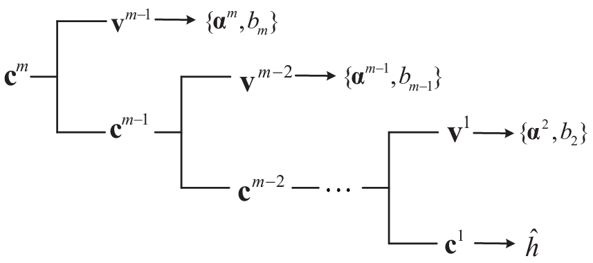
Firstly, we split the received signal into two length- parts and denote them as and , respectively. According to the nested structure summarized in (8), the elements of these two partial sequences are given by
Then, we perform the element-wise conjugate multiplication on them, i.e.,
| (9) |
where
As shown in (7), is a Walsh sequence with frequency . Hence, can be recovered by performing the Walsh-Hadamard Transformation (WHT) on (9). Specifically, the -th order Hadamard matrix is represented as and its elements are . Note that the Hadamard matrix we used here is obtained by flipping the normalized one, whose element is , up and down. We denote the result of the transformation by the vector , whose -th entry is
| (10) | ||||
where . Thus, when we have , will achieve its maximum value, which equals to . On this basis, the vector can be recovered by searching through the vector for the component having the largest value. Additionally, for simplicity, we can opt for comparing the real parts of with no performance loss. Specifically, with
and representing the real component, the estimate is the -bit binary expression of and then is the modulo-2 addition of the entries in , i.e.,
| (11) |
Next, combining the estimate and the pair of partial sequences and , we arrive at:
| (12) |
Under the condition that the estimate is correct, it is derived that
| (13) |
where .
In the sequel, the sequence is split into and and the estimates are calculated by repeating the above steps. This process continues until all the estimates and the length-2 sequence are obtained.
Then, the channel estimation can be done based on . Assuming that all the previous estimates are correct, we have
| (14) |
where
and the signs depend on the estimates . Since are i.i.d. random variables following the distribution , the channel coefficient can thus be estimated by
| (15) |
where according to (2).
Capitalizing on all the estimations above, the matrix-vector pair is recovered according to (5) and then reverts to the active user ID. To summarize, the layer-by-layer RM detection algorithm conceived for single sequence detection is presented in Algorithm 1.
Input:
the received signal ;
Output:
the matrix-vector pair , the channel coefficient .
However, we found that Algorithm 1 suffers from an error propagation problem. To elaborate, let us assume that an error occurs during the recovery of , which results in . Then the result of (12) turns out to be
| (16) | ||||
Since and are two different Walsh sequences, the cardinality of the set definitely equals to . As a result, the sequence loses half the information of , which will impose consistent errors in the following steps.
In the sequel, we propose a list detection algorithm for overcoming this error propagation problem. The algorithm can be partitioned into the extension and validation stages.
Firstly, let us consider the extension stage. For ease of clarification, we introduce two parameters , where determines the width of extension and , i.e., the number of elements in the vector , determines the depth of extension. On this basis, during the recovery of (line 4 of Algorithm 1), if , instead of choosing the location having the largest real component, we retain the most likely locations to obtain a series of candidates. Then, the detection is continued in these parallel threads, each called a detection path. For the list detection algorithm with parameters , the total number of the detection paths at the end equals to , and the path having the notation means that we choose the -th list in the -th layer along this path. Intuitively, if and , the list detection algorithm is equivalent to the classic maximum likelihood sequence estimation (MLSE), which achieves the optimal performance with a complexity that is super-linear to the size of the sequence space. Faced with the huge sequence space of RM sequences, the complexity of MLSE is excessive. In the proposed list detection algorithm, we keep track of several most likely paths to reach a compromise between complexity and performance. An example of list detection algorithm is illustrated in Fig. 6.

At the validation stage, the optimal path is chosen by measuring the residual sequence energy. To be specific, the residual sequence energy on the path is expressed as
| (17) |
Then the path having the minimum residual energy is decided to be the final detection result. The reasons to use the residual energy as the path metric are two fold. On one hand, it is intuitive that if the detected sequence actually exists, the residual energy should be reduced after it is canceled from the received signal. On the other hand, if errors occur during the detection process, the channel coefficient estimated by (15) can be proved to be a very small value. Specifically, if the algorithm is executed to the last step based on the result derived in (16), the sequence would have the form
Since there is little chance that is satisfied for every when errors occurred in the previous layers, we have and then according to (15). Hence, the result calculated by (17) is almost equal to the energy of the received signal and the corresponding path will be discarded.
IV-B Multi-Sequence Scenario: Iterative RM Detection and Channel Estimation Algorithm
In this section, we consider the scenario where multiple active users coexist in the system. We detect the RM sequences and estimate the channel coefficients in an iterative manner. The process is described in detail below.
We first introduce some notations. The maximum number of detected users is limited to . On one hand, a small value of would undoubtedly result in the unsatisfactory successful detection probability. On the other hand, if is set to be too large, it may cause high false alarm rate (FAR) and computational complexity. Hence, the choice of the exact value of is determined by the trade-off between the successful detection probability and the tolerable FAR, as well as the practical complexity constraint of the system. For ease of exposition, the superscripts in and are dropped. The stage where the RM sequence of the detected user is updated during the -th iteration is denoted as Stage . Furthermore, and represent the RM detection result and the channel estimate at Stage , respectively.
Firstly, we initialize the RM sequence and the channel coefficient as and , respectively. At Stage , the multiple access interference (MAI) is expressed as
| (18) |
where
Then, the result of is input to Algorithm 1 to obtain and .
Next, after all the detected users’ RM sequences are updated in this iteration, the results are fed to the linear least square channel estimator for further improving their accuracy, which is specified as
| (19) | ||||
Thanks to the information exchange between the sequence detector and the channel estimator, the performance gradually improves and the algorithm is terminated when the results are converged or the maximum number of iteration is reached. The multi-sequence detection procedure is summarized in Algorithm 2.
Input:
the received signal ,
the maximum number of iteration ,
the maximum number of detected users .
Output:
the active user ID set ,
the channel coefficient .
V Performance Analysis
V-A Performance of Layer-by-Layer RM Detection Algorithm
V-A1 Successful Detection Probability
Without loss of generality, we assume that the transmitted RM sequence is and the elements of the received signal are statistically independent. To derive the successful detection probability of single sequence detection algorithm, we consider the layer-by-layer recovery and the following theorem concludes the correct recovery probability of each layer.
Theorem 2: Under the circumstance that we have recovered correctly, the estimates are correct with the probability of
| (20) |
where ,
and is the distribution function of the standard normal distribution.
Proof:
In the sequel, we prove Theorem 2 by induction. Firstly, let us consider the case of . Recall that are i.i.d. random variables following . Given the channel coefficient , the received signal obeys . Then, upon approximating in (9) by a complex Gaussian variable with mean and variance , we see that follows the distribution .
Next, the Walsh-Hadamard transformation is performed on and the result is shown in (10). When , we have
| (21) |
while at other locations, i.e., , we arrive at:
| (22) |
Since is recovered by searching for the specific element with the largest real component, once there exists some that results in the event , the detection will head in the wrong direction. On the basis of (21) and (22), the probability of the event is
and the estimates are correct with the probability
| (23) |
Using the classic union bound as the upper bound of the second term in (23) and considering that the probability cannot be less than 0, we have that
| (24) | ||||
which is in accordance with (20).
Next, assuming that also agrees with (20) and the estimated are correct, is calculated as
| (25) |
where . With the knowledge that follows the distribution , we have that . The following derivation is similar to the case of and will not be repeated here due to space limitations. Finally, we can draw the conclusion that the correct detection probability of is identical to (20). ∎
The RM sequence is detected successfully only if each layer is correctly recovered, hence, its successful detection probability is formulated as
As for the list detection algorithm, it is clear that its performance is expected to be better than that of Algorithm 1, but inferior to that of MLSE.
Remark. Taking a second look at the noise term in (25) , we have:
where we find that the noise level decreases at an exponential rate layer by layer. Thus, if the first few layers are recovered correctly, the subsequent recovery will be correct with a high probability. This finding reveals the necessity to ensure the correctness of the first few layers. Inspired by this, to obtain a better detection performance in the list detection algorithm, we can increase the number of lists for the first few layers, while fixing the total number of paths.
V-A2 Computational Complexity
In the Layer-by-Layer RM detection algorithm, the Walsh-Hadamard transformation (WHT) plays the main role in the computational tasks. Thus, we firstly consider the multiplication operations of the WHT. Thanks to the recursive structure of the Walsh function, a fast WHT can be utilized to reduce the complexity, which takes multiplications when performed on a length- sequence. Hence, when only the WHT operations are considered, the total complexity of Algorithm 1 is . By contrast, the algorithm given in [16] exhibits a complexity order up to . This is due to the fact that the algorithm in [16] needs a length- fast WHT to recover each column of the matrix , while in Algorithm 1, the fast WHT is performed on , whose length is decreasing exponentially layer by layer. Hence, our proposed Algorithm 1 has significant advantage on complexity. If we further take the multiplications in Eq. (9) and Eq. (12) into account, the complexity of Algorithm 1 and the algorithm in [16] is and , respectively.
It is intuitive that the list detection algorithm improves the performance at the cost of an increased complexity. For the list detection algorithm, the number of multiplications is given by
Zhang et al. [17] proposed a shuffled version of the algorithm in [16] , which aims to improve the performance by changing the recovery order of the columns of the matrix . When the number of shuffles is , the complexity of this enhanced algorithm equals to .
Moreover, it is worth to mention the channel estimation complexity difference between these algorithms. When executed all the way to the last step, Algorithm 1 can directly estimate the channel coefficients according to (15). While the algorithms proposed in [16] and [17] cannot compute the channel coefficients and an extra least square (LS) estimation problem has to be solved, which incurs additional computational complexity.
V-B Performance of the Iterative RM Detection and Channel Estimation Algorithm
For ease of clarification, we analyze the performance in the case of . At Stage , the input of Algorithm 1 is exactly the received signal, i.e.,
| (26) |
After splitting it into a pair of partial sequences and computing their element-wise conjugate multiplication, we have
| (27) | ||||
where follows the distribution and . Then, the Walsh-Hadamard transformation is applied to (27) for obtaining the vector . Under the assumption that , is recovered correctly if and only if is satisfied for every , where is the location index that satisfies .
Firstly, in the special case of , the real component of the element at the location turns out to be
| (28) | ||||
The benefit of our proposed mapping rule manifests itself here. It is obvious from (28) that if , the component will decrease to and there is a substantial chance that it will become smaller than the other interference components, which results in the incorrect recovery of . While our constraint in (2) ensures that in this case and the magnitude of is reinforced to be
| (29) |
which is expected to improve the detection performance.
Next, in the case of , the real component of the element is specified as
| (30) | ||||
where . The second term of (30) happens to be the inner product of and , which is denoted as . Then, Eq. (30) can be recast as
| (31) |
Similarly, we have that
While at the location , the real component is expressed as
recalling that is the element of the Hadamard matrix . To proceed, we recast the first term as follows:
where denotes the inner product of and the RM sequence generated by the matrix-vector expressed as
and is obtained in the similar way.
It is obvious that the inner products of the RM sequences play an important role in determining the performance of multi-sequence detection. The authors of [16] reveal that the distribution of the inner products of second-order RM sequences is symmetric. Moreover, if two distinct matrices and satisfy that
then the magnitude of the inner product of their respective generated RM sequences is either or . This inspires us to restrict the matrices, for example, to be taken from the set [18], for further improving the attainable performance of RM detection.
Then, on the premise that is correctly recovered, the sequence is given as
where . Combined with (26), it is found that for the first active user, the signal-to-interference-and-noise-ratio (SINR) is enhanced. Furthermore, as the algorithm proceeds, the SINR of , which is denoted as , doubles layer by layer, specifically,
| (34) |
This finding further underlines the necessity of ensuring the correctness of the first few layers.
At the end of Stage , the estimates and are obtained. Then we enter Stage . At the beginning of Stage , the residual signal is calculated by
| (35) |
which is then input to Algorithm 1. The accuracy of both and affects the performance at this stage. If the sequence is correct, the impact of the channel estimation error (CEE) is relatively small. On one hand, in the case that are all correctly recovered, the SINR of the last layer is up to according to (34), which ensures that the CEE will not be too high. On the other hand, the LS channel estimator at the end of the first iteration is capable of further improving the accuracy of , and the second user’s RM sequence can be updated in the second iteration.
Whereas if the sequence is incorrect, (35) is equivalent to adding an extra sequence to the original received signal, which further lower the SINR. In [16] and [17], a traditional SIC-based method is used for multi-sequence detection . Explicitly, before detecting the next sequence, all the sequences obtained so far are subtracted from the received signal. In this scheme, the impact of any incorrectly detected sequences always persists. By contrast, the iterative method adopted in our proposed algorithm deals with this problem in a better way. For example, if the detected sequence is wrong but happens to be right, then at Stage , after subtracting the MAI term, the signal input to Algorithm 1 is equal to
which is free from the impact of the incorrect result and . Moreover, the algorithms in [16] and [17] need to perform LS channel estimation after each sequence detection, while our proposed algorithm executes LS channel estimation only once in an iteration, which further reduces the complexity.
Finally, the properties of our proposed algorithms are summarized as follows:
- •
As a benefit of the proposed mapping method, the channel coefficients can be estimated directly according to (15), which leads to a reduced computational complexity without any performance loss.
- •
In the case where multiple active users possess the same , our proposed mapping rule ensures that the corresponding result of the WHT is reinforced like in (V-B). As such, the successful recovery probability of is expected to be enhanced.
- •
By exploiting the nested structure of RM sequences, the matrix-vector pair is recovered layer by layer. During this process, the interference and noise level is found to keep on decreasing on the premise that are recovered correctly. On one hand, this ensures the accuracy of channel estimation based on (15). On the other hand, this reminds us of the importance of improving the recovery reliability of the first few layers. Inspired by this, we can adjust the parameters of the list detection algorithm for enhancing the performance.
- •
The inner products of RM sequences have a significant influence on the performance of multi-sequence detection. Motivated by this, we can further restrict the choice of the matrices to enhance detection capability. Intuitively, this is achieved at the cost of shrinking the user space size.
- •
In contrast to the common SIC-based detection, the iterative detection algorithm utilized in this paper is capable of reducing the impact of incorrectly detected sequences, thus it has a better capability to deal with the error propagation problem of SIC.
VI Simulation Results
In this section, we evaluate the performance of the proposed algorithms in terms of their sequence detection accuracy, channel estimation accuracy and computational cost. For ease of exposition, Algorithm 1 and its list detection version are denoted as “RM_LLD” and “list RM_LLD”, respectively. Moreover, the algorithm in [16] is used as the benchmark. Since it is based on the application of shift-and-multiply to the received signal, we referred to it and its shuffled version proposed in [17] as “RM_SMD” and “RM_SMD with shuffle”, respectively. In the sequel, the successful detection probability is defined as the average ratio between the number of successfully detected active users and the total number of active users in the system. The channel estimation error is quantified by the mean square error of channel estimates of successfully detected active users.
VI-A Performance of the Layer-by-Layer RM Detection Algorithm
Firstly, we examine the performance of the proposed algorithms in the single-sequence scenario. The simulation parameters are listed in Table. I.
| Sequence Length | |
| SNR | dB |
| Shuffle Times in “RM_SMD with shuffle” | 4 |
| of “list RM_LLD” | |
| Simulation Times |
Fig. 7 illustrates the successful detection probability versus the signal to noise ratio (SNR). It can be observed that RM_SMD faces severe performance degradation in the low-SNR scenario, while RM_LLD exhibits robustness against the SNR, thus confirming the superior detection performance of the proposed algorithm. As expected, both the shuffling operation and the list detection approach are capable of improving the detection performance. Even though both RM_SMD with 4 shuffles and list RM_LLD with choose the optimal result from 4 candidates, it is shown in Fig. 7 that list RM_LLD with is superior. Moreover, the theoretical results obtained in Section V.A is also depicted in Fig. 7. Since the union bound is utilized in the analysis, this result can act as the lower bound. The simulation result of RM_LLD and the theoretical result consistently show that when the SNR is higher than dB, the RM sequence can be successfully detected with a probability close to .

The computational complexity of these four algorithms associated with is compared in Table II. Here we quantify the complexity by the number of multiplication operations. Observe that the proposed RM_LLD impose a much lower complexity than RM_SMD. It is intuitive that both the list detection approach and the shuffle operation improve the performance at the cost of an increased complexity. However, the complexity of RM_SMD with shuffles increases linearly with the number of shuffles, while the complexity growth rate of list RM_LLD is much more gradual.
| Algorithm | Computational Complexity |
| RM_LLD | 2304 |
| list RM_LLD, | 3820 |
| RM_SMD | 35328 |
| RM_SMD, 4 shuffles | 141312 |
Finally, we verify the feasibility of estimating the channel coefficients according to (15). Fig. 8 depicts the channel estimation errors calculated both from Eq. (15) and by the least square (LS) estimator. It can be seen from Fig. 8 that the channel estimates calculated by (15) exhibit the same accuracy as the results obtained by the LS estimator. However, it is obvious that the complexity of (15) is much lower, which further validates the superiority of our proposed algorithm.

VI-B Performance of the iterative RM Detection and Channel Estimation Algorithm
Next, we evaluate the performance of our algorithms in the multi-sequence scenario and the corresponding parameters are summarized in Table. III.
| Sequence Length | , | |||||
| SNR | dB | |||||
|
5 | |||||
| False Alarm Rate | ||||||
|
| |||||
|
| |||||
| Simulation Times |


The successful detection probability versus the number of active users in the case of and is depicted in Fig. 9. It can be observed that the RM_SMD curve drops rapidly when increasing the number of active users, while RM_LLD shows a significant advantage over it. As in the single sequence scenario, both “RM_SMD with shuffle” and “list RM_LLD” improve the successful detection probability. Comparing the successful detection probability of “list RM_LLD, ” and “list RM_LLD, ”, we find that with the total number of paths fixed, the performance can be beneficially improved by increasing the number of lists in the first layer. This result further validates the importance of ensuring the reliable recovery of the first few layers in the proposed RM detection algorithm. Moreover, it can be seen from Fig. 9 that the iterative method adopted by our proposed algorithm is superior to the traditional SIC-based multi-sequence detection. This performance improvement is an explicit benefit of the mutual information exchange between the RM detector and the channel estimator as well as of the capability to eliminate the impact of incorrectly detected sequences. Combining Fig. 9(a) and (b), it is also clear that the detection capability is enhanced by increasing the length of sequences.

Fig. 10 compares the channel estimate error of different algorithms in the multi-sequence scenario when . An insightful observation is that although the successful detection probability of “list RM_LLD, SIC-based” and “list RM_LLD, iterative” seems similar in Fig. 9 (a), the channel estimates of “list RM_LLD, iterative” are obviously more accurate than those of “list RM_LLD, SIC-based”. Furthermore, the advantage of the iterative method becomes more prominent for “list RM_LLD, ” and “list RM_LLD, ”. Based on these results, we may conclude that the proposed iterative RM detection and channel estimation algorithm beneficially improves the user detection and channel estimation performance.
Fig. 11 depicts the convergence of the iterative RM detection and channel estimation algorithm for . It can be seen that the convergence rate is related to the number of active users in the system. In the case of , the algorithm can converge within iterations. Although it needs more iterations to converge when the number of active users increases, the successful detection probability keeps rising before achieving the convergence. Hence, the value of can be set according to the practical tradeoff between the detection capability and the complexity.

VII Conclusions
In this paper, we utilize RM sequences for user identification and channel estimation to meet the massive connectivity and low latency requirements of mMTC scenarios. A novel mapping rule was conceived for improving RM detection capability and for simplifying the channel estimation with no loss of accuracy. At the receiver, a layer-by-layer RM detection algorithm and an enhanced algorithm were invoked for single sequence detection. They are based on the nested structure of RM sequences, which is discovered to reveal the deeper relationship between their sub-sequences. Then an iterative RM detection and channel estimation algorithm was also designed for the case where multiple active users co-exist in the system. From the simulation results, our proposed algorithms have a significant advantage over existing ones in terms of detection performance and computational complexity.
References
- [1] ITU-R Rec. M.2083-0, ¡°IMT Vision - Framework and Overall Objectives of the Future Development of IMT for 2020 and Beyond,¡± Sept. 2015.
- [2] Huawei, 5G Network Architecture-A High-Level Perspective, 2016, white paper at Huawei.com.
- [3] 3GPP technical specifications 36.321. Evolved Universal Terrestrial Radio Access (E-UTRA); Medium Access Control (MAC). Available at: www.3gpp.org.
- [4] 3GPP technical specifications 36.211. Evolved Universal Terrestrial Radio Access (E-UTRA); Physical channels and modulation. Available at: www.3gpp.org.
- [5] G. Durisi, T. Koch, and P. Popovski, “Towards Massive, Ultra-Reliable, and Low-Latency Wireless Communication with Short Packets,” Proc. IEEE, vol. 104, no. 9, pp. 1711-1726, 2016.
- [6] H. S. Jang, S. M. Kim, K. S. Ko, J. Cha, and D. K. Sung, “Spatial group based random access for M2M communications,” IEEE Commun. Lett., vol. 18, no. 6, pp. 961-964, 2014.
- [7] S. Kim, H. Kim, H. Noh, Y. Kim, and D. Hongy, “Novel Transceiver Architecture for an Asynchronous Grant-free NOMA System,” unpublished.
- [8] N. K. Pratas, H. Thomsen, C. Stefanovic, and P. Popovski, “Code-Expanded Random Access for Machine-Type Communications,” in IEEE Globecom Workshops (GC Wkshps), Anaheim, 2012, pp. 1681-1686.
- [9] E. J. Candes and T. Tao, “Decoding by linear programming,” IEEE Trans. Inf. Theory, vol. 51, no. 12, pp. 4203-4215, 2005.
- [10] L. Liu and W. Yu, “Massive Connectivity With Massive MIMO-Part I: Device Activity Detection and Channel Estimation,” IEEE Trans. Signal Process., vol. 66, no. 11, pp. 2933-2946, 2018.
- [11] G. Wunder, P. Jung, and M. Ramadan, “Compressive Random Access Using a Common Overloaded Control Channel,” in IEEE Globecom Workshops (GC Wkshps), San Diego, 2015, pp. 1-6.
- [12] H. F. Schepker, C. Bockelmann, and A. Dekorsy, “Exploiting Sparsity in Channel and Data Estimation for Sporadic Multi-User Communication,” in Tenth Int. Symp. Wireless Commun. Syst., Ilmenau, 2013, pp. 1-5.
- [13] G. Hannak, M. Mayer, A. Jung, G. Matz, and N. Goertz, “Joint channel estimation and activity detection for multiuser communication systems,” in IEEE Int. Conf. Commun. Workshop (ICCW), London, 2015, pp. 2086-2091.
- [14] Z. Chen and W. Yu, “Massive device activity detection by approximate message passing,” in IEEE Int. Conf. Acoust., Speech and Signal Process. (ICASSP), New Orleans, 2017, pp. 3514-3518.
- [15] N. K. Pratas, C. Stefanovic, G. C. Madueno and P. Popovski, “Random Access for Machine-Type Communication Based on Bloom Filtering,” in IEEE Global Commun. Conf. (GLOBECOM), Washington, 2016, pp. 1-7.
- [16] S. D. Howard, A. R. Calderbank, and S. J. Searle, “A fast reconstruction algorithm for deterministic compressive sensing using second order reed-muller codes,” in 42nd Annu. Conf. Inf. Sci. and Sys., Princeton, 2008, pp. 11-15.
- [17] H. Zhang, R. Li, J. Wang, Y. Chen and Z. Zhang, “Reed-Muller Sequences for 5G Grant-Free Massive Access,” in IEEE Global Commun. Conf., Singapore, 2017, pp. 1-7.
- [18] A. Calderbank and S. Jafarpour, “Reed Muller sensing matrices and the LASSO,” in Int. Conf. Sequences Their Applicat. (SETA), Paris, 2010, pp. 442-463.