$L^{\infty}$ -estimation of generalized Thue-Morse trigonometric polynomials and ergodic maximization

Aihua FAN Address: LAMFA, UMR 7352 CNRS, University of Picardie, 33 rue Saint Leu, 80039 Amiens, France Email address: ai-hua.fan@u-picardie.fr , JÖRG SCHMELING Address: Lund University
Centre for Mathematical Sciences
Box 118, 221 00 LUND, Sweden Email address: joerg@maths.lth.se and Weixiao SHEN Address: Shanghai Center for Mathematical Sciences
Fudan University
220 Handan Road, Shanghai 200433, China Email address: wxshen@fudan.edu.cn

Abstract.

Given an integer $q\geq 2$ and a real number $c\in[0,1)$ , consider the generalized Thue-Morse sequence $(t_{n}^{(q;c)})_{n\geq 0}$ defined by $t_{n}^{(q;c)}=e^{2\pi icS_{q}(n)}$ , where $S_{q}(n)$ is the sum of digits of the $q$ -expansion of $n$ . We prove that the $L^{\infty}$ -norm of the trigonometric polynomials $\sigma_{N}^{(q;c)}(x):=\sum_{n=0}^{N-1}t_{n}^{(q;c)}e^{2\pi inx}$ , behaves like $N^{\gamma(q;c)}$ , where $\gamma(q;c)$ is equal to the dynamical maximal value of $\log_{q}\left|\frac{\sin q\pi(x+c)}{\sin\pi(x+c)}\right|$ relative to the dynamics $x\mapsto qx\mod 1$ and that the maximum value is attained by a $q$ -Sturmian measure. Numerical values of $\gamma(q;c)$ can be computed.

1. Introduction and main results

Let $q\geq 2$ be a positive integer. For any integer $n\geq 0$ , we denote by $S_{q}(n)$ the sum of digits of expansion of $n$ in base $q$ . Fix $c\in[0,1)$ , we define the generalized Thue-Morse sequence $(t_{n}^{(q;c)})_{n\geq 0}$ by

t_{n}^{(q;c)}=e^{2\pi icS_{q}(n)}.

The case that $q=2$ and $c=1/2$ corresponds to the classical Thue-Morse sequence:

1,-1,-1,1,-1,1,1,-1,-1,1,1,-1,1,-1,-1,1,\cdots.

By a generalized Thue-Morse trigonometric series we mean

\sum_{n=0}^{\infty}t_{n}^{(q;c)}e^{2\pi inx},

which defines a distribution on the circle $\mathbb{T}:=\mathbb{R}/\mathbb{Z}$ . We are interested in the asymptotic behaviors of its partial sums, called the generalized Thue-Morse trigonometric polynomials:

\sigma_{N}^{(q;c)}(x):=\sum_{n=0}^{N-1}t_{n}^{(q;c)}e^{2\pi inx}\quad(N\geq 1).

(1.1)

The first problem is to find or to estimate the best constant $\gamma$ such that

\sup_{x\in\mathbb{R}}\left|\sum_{n=0}^{N-1}t_{n}^{(q;c)}e^{2\pi inx}\right|=O(N^{\gamma}).

(1.2)

Define $\gamma(q,c)$ , sometimes denoted $\gamma(c)$ , to be the infimum of all $\gamma$ for which (1.2) holds. Following Fan [15], we call $\gamma(c)$ the Gelfond exponent of the generalized Thue-Morse sequence $(t^{(q;c)}_{n})$ . The first result, due to Gelfond [20], is that

\gamma(2;1/2)=\frac{\log 3}{\log 4}=0.792481....

Trivially $\gamma(q;0)=1$ . No other exact exponents $\gamma(q;c)$ are known. A basic fact, as a consequence of the so-called $q$ -multiplicativity of $(t^{(q;c)}_{n})$ , is the following expression

|\sigma_{q^{n}}^{(c)}(x)|=\prod_{k=0}^{n-1}\left|\frac{\sin\pi(q^{k}x+c)}{\sin\pi(x+c)}\right|.

(1.3)

Thus the dynamical system $T=T_{q}:\mathbb{T}\to\mathbb{T}$ defined by $Tx=qx\mod 1$ is naturally involved. Let

f_{q;c}(x):=f_{c}(x):=\log\left|\frac{\sin q\pi(x+c)}{\sin\pi(x+c)}\right|.

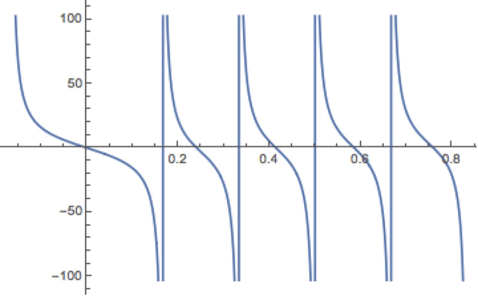
We will simply write $f_{c}$ if there is no confusion. Let us point out that $f_{c}$ is a translation of $f_{0}$ and that $f_{0}(x)\leq\log q$ for all $x$ and $f_{0}(0)=\log q$ , and $f_{0}$ has $q-1$ singularities as a function on $\mathbb{T}$ in the sense $f_{0}(r/q)=-\infty$ for $1\leq k\leq q-1$ . Furthermore, $f_{0}$ is concave between any two adjacent singularity points. Consequently $f_{c}$ attains its maximal value at $x=-c$ and its singularity points are $b_{k}:=-c+k/q$ ( $1\leq k\leq q-1$ ). See Figure 1 for its graph.

Refer to caption — Figure 1. The graphs of $f_{0}$ on the interval $[-1/q,1-1/q]$ , here $q=6$ .

As we shall see in Proposition 3.2, finding the Gelfond exponent $\gamma(c)=\gamma(q;c)$ is equivalent to maximizing $f_{c}$ . That is to say

\gamma(c)=\frac{\beta(c)}{\log q}

(1.4)

with

\beta(c):=\sup_{\mu\in\mathcal{M}_{T}}\int_{\mathbb{T}}f_{c}(x)d\mu(x)

(1.5)

where $\mathcal{M}_{T}$ is the set of $T$ -invariant Borel probability measures (Theorem 2.1). It is easy to see that $\gamma(c)<1$ so that $\beta(c)<\log q$ for all $c\in(0,1)$ , just because

\max_{x}\prod_{j=0}^{q-1}\left|\frac{\sin q\pi(q^{j}x+c)}{q\sin\pi(q^{j}x+c)}\right|<1.

A detailed argument is given in [16].

Our main result in this paper is the following theorem concerning the maximal value $\beta(c)$ .

Main Theorem. Fix an integer $q\geq 2$ . The following hold.
(1) The supremum in (1.5) defining $\beta(c)$ is attained by a unique measure and this measure is $q$ -Sturmian.
(2) Such a $q$ -Sturmian measure is periodic in most cases. More precisely, those parameters $c$ corresponding to non-periodic Sturmian measures form a set of zero Hausdorff dimension.
(3) There is a constant $C>0$ such that

\forall x\in\mathbb{T},\forall N\geq 1,\ \ \ \left|\sum_{n=0}^{N-1}t_{n}^{(q;c)}e^{2\pi inx}\right|\leq CN^{\gamma(c)}.

(1.6)

A $q$ -Sturmian measure is by definition a $T_{q}$ -invariant Borel probability measure with its support contained in a closed arc of length $\frac{1}{q}$ . It is well-known that each closed arc of length $\frac{1}{q}$ supports a unique $T$ -invariant Borel probability measure. A proof of this fact is included in Appendix A for the reader’s convenience.

For the maximization, many of the existing results in the literature deal with the case that $f$ is a Hölder continuous function, by Bousch [6, 7], Jenkinson [24, 25, 26, 27], Jenkinson and Steel [28], Contreras, Lopes and Thieullen [11], Contreras [12], among others. There is a very nice survey paper [23] in which there is a rather complete list of references. See also Anagnostopoulou et al [2, 3, 4], Bochi [5].

Up to now, as far as we know, only the exact value of the Gelfond exponent $\gamma(2;1/2)$ is known, obtained by Gelfond [20]. Some estimate is obtained by Mauduit, Rivat and Sarkozy [34]. In Section 7, a computer-aided method will be provided to compute the Gelfond exponent $\gamma(c)$ , based on the theory developed in Section 4. Figure 2 shows the graph of $\gamma(2;c)$ for $c$ ’s corresponding to periodic Sturmian measures with period not exceeding $13$ . More details can be filled in by using Sturmian measures with larger periods. Let us point out that for $c\in(0.428133329021334,0.571866670978666)$ , we get the exact value

\beta(2;c)=\log 2+\frac{1}{2}\log\left|\cos\pi\left(\frac{1}{3}+c\right)\cos\pi\left(\frac{2}{3}+c\right)\right|.

(1.7)

The modal around $c=\frac{1}{2}$ of the graph of $\beta(\cdot)$ is nothing but the graph of the function on the right hand side of (1.7). This is the contribution of the $2$ -cycle $\{1/3,2/3\}$ . Other details shown in Figure 2 are contributed by other cycles. See (7.3) for a formula more general than (1.7). The symmetry of the graph of $\gamma(\cdot)$ reflects nothing but the fact $\gamma(q;1-c)=\gamma(q;c)$ which holds for all $c$ .

The Thue-Morse sequence $t_{n}^{(2;1/2)}=(-1)^{s_{2}(n)}$ and the digital sum function $n\mapsto s_{2}(n)$ are extensively studied in harmonic analysis and number theory after the works of Mahler [31] and Gelfond [20]. The set of natural numbers $n$ such that $s_{2}(n)$ are even is studied and the norms $\|\sigma_{N}^{(c)}\|_{\infty}$ and $\|\sigma_{N}^{(c)}\|_{1}$ are involved in the study of the distribution of such sets in $\mathbb{N}$ [20, 19, 18, 14]. Queffélec [36] showed how to estimate the $L^{1}$ -norm using the $L^{\infty}$ -norm through an interpolation method. C. Mauduit and J. Rivat [33] answered a longstanding question of A. O. Gelfond [20] on how the sums of digits of primes are distributed. This study deals with $\sum_{p\leq N}e^{2\pi ixs_{2}(p)}$ ( $p$ being prime). Polynomials of the form $\sum_{n\leq N}(1+(-1)^{s_{2}(n)})e^{2\pi inx}$ are studied in [1]. Recently Fan and Konieczny [16] proved that for every $0<c<1$ and every integer $d\geq 1$ there exist constants $C>0$ and $0<\gamma_{d}<1$ such that

\sup_{\begin{subarray}{c}q\in\mathbb{R}[x]\\ \deg q\leq d\end{subarray}}\left|\sum_{n=0}^{N-1}t_{n}^{(c)}e^{2\pi iq(n)}\right|\leq CN^{\gamma_{d}}.

See also [29]. But the optimal $\gamma_{d}$ is not known.

A dual quantity is the minimal value

\alpha(c):=\inf_{\mu\in\mathcal{M}_{T}}\int_{\mathbb{T}}f_{c}(x)d\mu(x)

(1.8)

which will play an important role in the study of the pointwise behavior of $\sigma_{N}^{(q;c)}(x)$ . This minimization and the multifractal analysis of $\sigma_{N}^{(q;c)}(x)$ are stuided in a forthcoming paper.

We start the paper with a general setting of dynamical maximization and minimization (Section 2) and an observation that the computation of the Gelfond exponents for generalized Thue-Morse sequences is a dynamical maximization problem (Section 3). Theorem A will be proved in Section 4 which is the core of the paper. Section 5 is an appendix, devoted to the numerical computation of $\beta(c)$ and $\gamma(c)$ .

Acknowledgements. The authors are grateful to Thierry Bousch and Oliver Jenkinson for providing useful informations, to Geng Chen for numerical computation and graphic generation. The first author is supported by NSFC grant no. 11471132 and the third author is supported by NSFC grant no. 11731003. The first and second authors would like to thank Knuth and Alice Wallenberg Foundation and Institut Mittag-Leffler (Sweden) for their supports.

2. General setting of maximization and minimization

Let $T:X\to X$ be a continuous map from a compact metric space $X$ to itself. Given an upper semi-continuous function $f:X\to[-\infty,+\infty)$ , an interesting and natural problem is ergodic optimization which asks for the following maximization

\beta_{f}:=\sup_{\mu\in\mathcal{M}_{T}}\int f(x)d\mu(x)

(2.1)

where $\mathcal{M}_{T}$ denotes the convex set of all Borel probability $T$ -invariant measures. An $f$ -maximizing measure is by definition a probability invariant measure attaining the maximum in (2.1).

What we shall be mostly interested in is as follows: $X$ is the circle $\mathbb{T}=\mathbb{R}/\mathbb{Z}$ , $Tx=qx\mod 1$ for some integer $q\geq 2$ , and

f(x)=\log|\varphi(x)|,

where $\varphi:X\to\mathbb{R}$ is an analytic function not identically zero and moreover,

\varphi^{\prime\prime}(x)\varphi(x)<\varphi(x)^{2}

whenever $\varphi(x)\not=0$ . That is to say, on any interval where $\varphi(x)\not=0$ , $\log|\varphi|$ is concave. Such a function $f$ has only singularities of logarithm type, i.e. if $b$ is a singular point then

\log\varphi(x)\asymp\log|x-b|

holds in a neighborhood of $b$ . A typical example is $\varphi(x)=\frac{\sin\pi q(x+c)}{\sin\pi(x+c)}$ (see Figure 3).

2.1. Maximization

The points (1) and (2) in the following theorem were proved by Jenkinson [24]. They were discussed in [13] for continuous function $f$ . The point (2) provides three different ways to describe the maximization (2.1) through time averages along orbits. The point (3) provides a fourth way, using periodic points, in the case of the dynamics $T_{q}$ .

Let $R(f)$ be the set of $x$ such $\lim_{n}n^{-1}S_{n}f(x)$ exists, where

S_{n}f(x)=\sum_{k=0}^{n-1}f(T^{k}x).

Theorem 2.1.

Suppose that $f$ is upper semi-continuous.
(1) The map $\mu\mapsto\int fd\mu$ is upper semi-continuous so that the supremum in (2.1) defining $\beta_{f}$ is attained.
(2) The maximum value $\beta_{f}$ is equal to

\sup_{x\in R(f)}\lim_{n\to\infty}\frac{S_{n}f(x)}{n}=\sup_{x\in X}\limsup_{n\to\infty}\frac{S_{n}f(x)}{n}=\lim_{n\to\infty}\max_{x}\frac{S_{n}f(x)}{n}.

(3) Assume $X=\mathbb{T}$ , $T(x)=qx\mod 1$ , and $f(x)=\log|\varphi(x)|$ with $\varphi$ an analytic function having a finite number of zeros. We have

\beta_{\log|\varphi|}=\sup_{\mu\in\mathcal{P}_{T}}\int\log|\varphi|d\mu,

(2.2)

where $\mathcal{P}_{T}$ denote the collection of all $T$ -invariant probability measures supported on periodic orbits.

Proof.

(1) and (2) were proved in [24]. Here we only give an explanation that the last limit in (2) exists. Indeed, putting $S_{n}=\max_{x\in X}S_{n}f(x)$ , we have $S_{n+m}\leq S_{n}+S_{m}$ , so the limit exists.

(3) Let us prove (2.2). Obviously the left hand side is not smaller than the right hand side. So it suffices to prove that for any $\mu\in\mathcal{M}_{T}$ with $\int\log|\varphi|d\mu=:\alpha>-\infty$ and any $\varepsilon>0$ , there exist a periodic point $p\in\mathbb{T}$ of period $s$ such that

\sum_{j=0}^{s-1}\log|\varphi(T^{j}p)|\geq s(\alpha-\varepsilon).

(2.3)

By the ergodic decomposition, we may assume that $\mu$ is ergodic.

We first prove the following claim.
Claim. Let $\mathcal{C}$ denote the set of zeros of $\varphi$ . There exists $\delta_{0}>0$ such that for $\mu$ -a.e. $x\in\mathbb{T}$ , there exists an arbitrarily large positive integer $N$ such that

d(T^{j}(x),\mathcal{C})\geq q^{-(N-j)}\delta_{0}\mbox{ for all }0\leq j<N.

To prove the claim, let $\mathcal{C}_{\delta}:=\{x:d(x,\mathcal{C})<\delta\}$ be the $\delta$ -neighbourhood of $\mathcal{C}$ . Since $\log|\varphi|$ is $\mu$ -integrable, we must have $\mu(\mathcal{C})=0$ and then $\int_{\mathcal{C}_{\delta}}\log|\varphi|d\mu\to 0$ as $\delta\to 0$ . Put

\text{dep}_{\delta}(x)=\left\{\begin{array}[]{ll}-\log_{q}d(x,\mathcal{C})&\mbox{ if }x\in\mathcal{C}_{\delta};\\ 0&\mbox{ otherwise.}\end{array}\right.

Since $\varphi$ is analytic and non-constant, for any $x_{0}\in\mathcal{C}$ we have

\log|\varphi(x)|=a+m\log d(x,x_{0})+o(1)\ \ \ {\rm as}\ \ x\to x_{0}

(2.4)

for some real number $a$ and integer $m\geq 1$ . Then there exist $\delta_{0}>0$ and $C>0$ such that

\text{dep}_{\delta}(x)\leq C|\log\varphi(x)|\quad(\forall\delta\in(0,\delta_{0}],\forall x\in\mathcal{C}_{\delta})

Then $\int_{\mathbb{T}}\text{dep}_{\delta}(x)d\mu\to 0$ as $\delta\to 0$ . Choose $\delta_{0}\in(0,1)$ such that

\int_{\mathbb{T}}\text{dep}_{\delta_{0}}(x)d\mu<\frac{1}{2}.

Since $\mu$ is ergodic, for $\mu$ -a.e. $x\in\mathbb{T}$ ,

\frac{1}{n}\sum_{i=0}^{n-1}\text{dep}_{\delta_{0}}(T^{i}x)<\frac{1}{2},\mbox{ when }n\gg 1.

(2.5)

By Pliss Lemma [35], it follows that there is an arbitrarily large integer $N$ such that for any $0\leq j<N$ ,

\sum_{i=j}^{N-1}\text{dep}_{\delta_{0}}(T^{i}(x))<N-j,

and in particular,

d(T^{j}(x),\mathcal{C})\geq\min(q^{-(N-j)},\delta_{0})\geq q^{-(N-j)}\delta_{0}.

(2.6)

The claim is proved.

Let us now complete the proof. Fix $\delta_{0}>0$ as we have chosen above and choose a point $x\in\mathbb{T}$ such that the conclusion of the Claim holds for a sequence of positive integers $N_{1}<N_{2}<\cdots$ . Choose $x$ suitably so that

\frac{1}{n}\sum_{i=0}^{n-1}\log|\varphi(T^{i}x)|\to\alpha,\mbox{ as }n\to\infty.

(2.7)

Given $\varepsilon>0$ , let $\eta>0$ be small such that

\forall y,y^{\prime}\in\mathbb{T},d(y,y^{\prime})<3\eta d(y,\mathcal{C})\Rightarrow|\log\varphi(y)-\log\varphi(y^{\prime})|<\frac{\varepsilon}{2}.

(2.8)

Let $z$ be an accumulation point of $\{T^{N_{k}}(x)\}_{k=1}^{\infty}$ . First fix $k_{0}$ such that $d(z,T^{N_{k_{0}}}(x))<\eta\delta_{0}$ . Then find $k\gg k_{0}$ such that $d(T^{N_{k}}(x),z)<\eta\delta_{0}$ and

\frac{1}{s}\sum_{j=0}^{s-1}\log|\varphi(T^{j}(y))|>\alpha-\frac{\varepsilon}{2},

where $y=T^{N_{k_{0}}}(x)$ and $s=N_{k}-N_{k_{0}}$ . Then

d(T^{j}(y),\mathcal{C})\geq q^{-(s-j)}\delta_{0}\quad(\forall 0\leq j<s).

(2.9)

We can choose $N_{k_{0}}$ and $N_{k}$ such that $q^{-s}<\eta$ .

Let $J:=[y-q^{-s}\delta_{0},y+q^{-s}\delta_{0}]$ . Since $T^{s}$ maps J bijectively onto $[T^{s}(y)-\delta_{0},T^{s}(y)+\delta_{0}]\supset J$ , there exists $p\in J$ such that $T^{s}(p)=p$ . Notice that for $0\leq j<s$ ,

d(T^{j}(y),T^{j}(p))=q^{-(s-j)}d(T^{s}y,p)<q^{-s+j}\cdot 3\eta\delta_{0}<3\eta d(T^{j}(y),\mathcal{C}),

because $d(T^{s}y,z)<\eta\delta_{0}$ , $d(z,y)<\eta\delta_{0}$ and $d(y,p)\leq q^{-s}\delta_{0}<\eta\delta_{0}$ . For the last inequality we used (2.9). According to (2.8), this implies that

\log\varphi(T^{j}(p))-\log\varphi(T^{j}(y))>-\frac{\varepsilon}{2}.\quad(\forall 0\leq j<s).

Therefore

\frac{1}{s}\sum_{j=0}^{s-1}\log\varphi(T^{j}(p))>\frac{1}{s}\sum_{j=0}^{s-1}\log\varphi(T^{j}(y))-\frac{\varepsilon}{2}>\alpha-\varepsilon.

Thus (2.3) is proved. ∎

3. Gelfond exponent and maximization problem

We approach the computation of Gelfond exponent from the point of ergodic optimization. Throughout we fix an integer $q\geq 2$ and will drop the superscript $q$ from notation. Recall that $T$ denotes the map $x\mapsto qx\mod 1$ on the circle $\mathbb{T}=\mathbb{R}/\mathbb{Z}$ . For each $c\in\mathbb{R}$ , put

f_{c}(x):=\log\varphi_{c}(x)\ {\rm with}\ \varphi_{c}(x)=\left|\frac{\sin\pi q(x+c)}{\sin\pi(x+c)}\right|.

So $\varphi_{c}(x)=\varphi_{0}(x+c)$ and $f_{c}(x)=f_{0}(x+c)$ .

Fix $x\in\mathbb{R}$ and consider the function $w_{x}^{(c)}:\mathbb{N}\to\mathbb{C}$ defined by

w_{x}^{(c)}(n):=t_{n}^{(c)}e^{2\pi inx}=e^{2\pi i(cS_{q}(n)+nx)},

which is $q$ -multiplicative in the sense that

w_{x}^{(c)}(aq^{t}+b)=w_{x}^{(c)}(aq^{t})w_{x}^{(c)}(b)

for all non-negative integers $a,b$ and $t$ such that $b<q^{t}$ (see [20]). Using this multiplicativity we can establish a relationship between Gelfond exponents and dynamical maximizations.

3.1. Gelfond exponent and maximization

Indeed, the $q$ -multiplicativity gives rise to

\sigma_{q^{n}}^{(c)}(x)=\prod_{k=0}^{n-1}\sum_{j=0}^{q-1}w_{x}^{(c)}(j\cdot q^{k}).

Since the above sum is equal to

\sum_{j=0}^{q-1}e^{2\pi ij(c+q^{k}x)}=\frac{1-e^{2\pi iq(c+q^{k}x)}}{1-e^{2\pi i(c+q^{k}x)}}=\frac{e^{\pi iq(c+q^{k}x)}}{e^{\pi i(c+q^{k}x)}}\frac{\sin\pi q(q^{k}x+c)}{\sin\pi(q^{k}x+c)},

we get

\left|\sigma_{q^{n}}^{(c)}(x)\right|=\prod_{k=0}^{n-1}\varphi_{c}(q^{k}x).

(3.1)

Therefore, (1.2) is equivalent to the following estimation:

\sup_{x\in\mathbb{R}}\prod_{j=0}^{n-1}\varphi_{c}(q^{j}x)=O(q^{n\gamma}).

(3.2)

In particular, $\gamma(c)$ is also the infimum of $\gamma$ for which (3.2) holds. The function $\gamma(\cdot)$ has the following symmetry.

Proposition 3.1.

We have $\gamma(c)=\gamma(1-c)$ for all $c\in[0,1]$ . Moreover, for all $n\geq 1$ and all $x\in[0,1]$ we have

\prod_{j=0}^{n-1}\varphi_{c}(q^{j}x)=\prod_{j=0}^{n-1}\varphi_{1-c}(q^{j}(1-x)).

Proof.

This follows simply from the parity and the $1$ -periodicity of $\varphi(x):=\varphi_{0}(x)$ which gives

\varphi(x+c)=\varphi(-x-c)=\varphi(-x+(1-c)),

and of the fact $-q^{n}x=q^{n}(1-x)\mod 1$ . ∎

By definition, the sequences $(t_{n}^{(2;3/4)})$ and $(t_{n}^{(2;1/4)})$ are related in the following way

\frac{t_{n}^{(2;3/4)}}{t_{n}^{(2;1/4)}}=t_{n}^{(2;1/2)}=(-1)^{S_{2}(n)}.

An amazing relation! Apparently, $(t_{n}^{(2;3/4)})$ and $(t_{n}^{(2;1/4)})$ seem very different, but $|\sigma_{2^{n}}^{(2;3/4)}(x)|=|\sigma_{2^{n}}^{(2;1/4)}(1-x)|$ .

Proposition 3.2.

We have $\gamma(c)=\frac{\beta(c)}{\log q}$ for each $c$ .

This is a consequence of (3.2) and Theorem 2.1.

4. Maximization for $f_{c}$ and Sturmian measures

In this section, we consider the maximizing problem in our most interesting particular case. Let $T$ denote the map $x\mapsto qx$ on the circle $\mathbb{T}=\mathbb{R}/\mathbb{Z}$ , and for each $c\in\mathbb{R}$ , put

f_{c}(x):=\log\varphi_{c}(x),\ \ \ {\rm with}\ \ \varphi_{c}(x)=\left|\frac{\sin\pi q(x+c)}{\sin\pi(x+c)}\right|.

Recall that our object of study is to find

\beta(c)=\sup_{\mu\in\mathcal{M}_{T}}\int_{\mathbb{T}}f_{c}d\mu.

For each $\lambda\in\mathbb{R}$ , there is a unique $T$ -invariant measure $\mathfrak{S}_{\lambda}$ that is supported in circle arc $C_{\lambda}:=[\lambda,\lambda+q^{-1}]$ $\mod 1$ , called $q$ -Sturmian measure. These measures $\mathfrak{S}_{\lambda}$ are ergodic and $\mathfrak{S}_{\lambda}=\mathfrak{S}_{\lambda^{\prime}}$ whenever $\lambda^{\prime}-\lambda\in\mathbb{Z}$ . See Appendix A for a proof of these facts.

The main result of this section is the following theorem.

Theorem 4.1.

Fix an integer $q\geq 2$ .For any $c\in\mathbb{R}$ , $f_{c}$ has a unique maximizing measure $\nu_{c}$ . The measure $\nu_{c}$ is a $q$ -Sturmian measure. Moreover, there exists a constant $C>0$ , which is independent of $c$ , such that

\sum_{i=0}^{n-1}f_{c}(q^{n}x)-n\beta(c)\leq C,

for each $x\in\mathbb{R}$ and each $n\geq 1$ .

To prove Theorem 4.1, we shall apply and extend the theory of Bousch-Jenkinson. An important fact that is used in the argument is that $f_{c}$ is strictly concave away from the singularties, or equivalently that is the same for $f_{0}$ :

f_{0}^{\prime\prime}(x)=\pi^{2}\left(\frac{1}{\sin^{2}\pi x}-\frac{q^{2}}{\sin^{2}\pi qx}\right)<0.

We shall first recall the pre-Sturmian and Sturmian condition introduced by Bousch [6]. Bousch introduced these concepts in the case $q=2$ which extends to the general case in a straightforward way.

4.1. Pre-Sturmian condition and Sturmian condition

For each $\gamma\in\mathbb{R}$ , let

C_{\gamma}:=[\gamma,\gamma+{1}/{q}]\mod 1\subset\mathbb{T}

be the arc in $\mathbb{T}$ , starting from $\gamma$ and rotating in the anti-clockwise direction. Let $C_{\gamma}^{\prime}=[\gamma,\gamma+1/q)\mod 1\subset\mathbb{T}$ and $\tau_{\gamma}:\mathbb{T}\to C_{\gamma}^{\prime}$ denote the inverse branch of $T$ restricted on $C_{\gamma}^{\prime}$ . So $\tau(Tx)$ is the unique point in $C_{\gamma}^{\prime}$ such that $q(\tau(Tx)-x)\in\mathbb{Z}$ .

The following definition comes from Bousch [6] which discusses the case $q=2$ with $f$ supposed Lipschitzian. We will only assume that $f$ is Lipschtzian on $C_{\lambda}$ .

Definition 4.1.

Let $f:\mathbb{T}\to[-\infty,+\infty)$ be a Borel function and let $\lambda\in\mathbb{R}$ . We say that $f$ satisfies the pre-q-Sturmian condition for $\lambda$ , if $f$ is Lipschitz on $C_{\lambda}$ and there exists a Lipschitz function $\psi:\mathbb{T}\to\mathbb{R}$ and a constant $\beta\in\mathbb{R}$ such that

\forall x\in C_{\lambda},\ f(x)+\psi(x)-\psi\circ T(x)=\beta.

(4.1)

If, furthermore,

\forall y\in\mathbb{T}\setminus{C}_{\lambda},\ f(y)+\psi(y)-\psi\circ T(y)<\beta,

(4.2)

then we say that $f$ satisfies the q-Sturmian condition for $\lambda$ .

To study the pre-Sturmian condition, let us consider the first time to leave $C_{\gamma}^{\prime}$

e_{\gamma}(x):=\inf\{k\geq 0:T^{k}x\in\mathbb{T}\setminus{C}_{\gamma}^{\prime}\}=\sum_{n=0}^{\infty}\chi_{\tau_{\gamma}^{n}(C_{\gamma}^{\prime})}(x).

(4.3)

Let $A_{1}=C_{\gamma}^{\prime}$ and $A_{n}=C_{\gamma}^{\prime}\cap T^{-1}A_{n-1}$ for $n>1$ . Then

A_{n}=C_{\gamma}^{\prime}\cap\tau_{\gamma}(C_{\gamma}^{\prime})\cap\cdots\cap\tau_{\gamma}^{n-1}(C_{\gamma}^{\prime})=\tau_{\gamma}^{n-1}(C_{\gamma}^{\prime}).

From this we verify the second equality in (4.3). Thus $e_{\gamma}\in L^{1}$ and

\int_{\mathbb{T}}e_{\gamma}(x)dx=\sum_{n=1}^{\infty}q^{-n}=\frac{1}{q-1}.

Since $\tau_{\gamma}(C_{\gamma}^{\prime})\subset C_{\gamma}^{\prime}$ , the function $e_{\gamma}$ is supported by $C_{\gamma}^{\prime}$ .

We have the following criterion for the pre-Sturmian condition, due to Bousch [6] (p.503).

Proposition 4.2.

Let $f:\mathbb{T}\to[-\infty,+\infty)$ be a Borel function bounded from above.

(1)

If $f$ satisfies the q-Sturmian condition on $C_{\lambda}$ for some $\lambda\in\mathbb{R}$ , then $\mathfrak{S}_{\lambda}$ is the unique maximizing measure of $f$ .
(2)

$f$ satisfies the pre-q-Sturmian condition for $\lambda$ if and only if $f$ is Lipschitzian on $C_{\lambda}$ and

$v_{f}(\lambda):=\int_{C_{\lambda}}f^{\prime}(x)e_{\lambda}(x)dx=0.$

Proof.

These results were stated in [6] for Lipschitzian $f$ . But only the Lipschtzian condition on $C_{\lambda}$ is actually needed. We repeat here the main lines of proofs for the convenience of reading.

(1) It is clear that $\beta$ is attained by the Sturmian measure. On the other hand, any other invariant measure $\mu$ has a support intersecting $\mathbb{T}\setminus C_{\lambda}$ , by the uniqueness of Sturmian measure supported by $C_{\lambda}$ . Then $\int fd\mu<\beta$ by the Sturmian condition.

(2) Let $\tau=\tau_{\lambda}$ . Assume the pre-Sturmain condition which can be restated as

\forall x\in\mathbb{T}\setminus\{q\lambda\},\quad\psi(x)=-\beta+\psi(\tau x)+f(\tau x).

By differentiating and iterating, we get

a.e.\ \ \forall N\geq 1,\quad\psi^{\prime}(x)=\sum_{n=1}^{N}\frac{f^{\prime}(\tau^{n}x)}{q^{n}}+\frac{\psi^{\prime}(\tau^{n}x)}{q^{N}}.

Since $\psi$ is Lipschitzian, $\psi^{\prime}$ exists almost everywhere and $\psi^{\prime}\in L^{\infty}(\mathbb{T})$ . Letting $N\to\infty$ , we get the following formula

a.e.\ \ \ \psi^{\prime}(x)=\sum_{n=1}^{\infty}\frac{f^{\prime}(\tau_{\lambda}^{n}x)}{q^{n}}.

(4.4)

Then integrate it to obtain

0=\psi(1)-\psi(0)=\int_{0}^{1}\psi^{\prime}(x)dx=\int_{C_{\lambda}}f^{\prime}(x)e_{\lambda}(x)dx.

(4.5)

Now assume $\int_{C_{\lambda}}f^{\prime}(x)e_{\lambda}(x)dx=0$ and $f$ is Lipschitzian on $C_{\lambda}$ . Then $f^{\prime}$ exists almost everywhere on $C_{\lambda}$ and $f^{\prime}\in L^{\infty}(C_{\lambda})$ . Since $f^{\prime}\in L^{\infty}(C_{\lambda})$ , the series in (4.4) defines a bounded function $\psi^{\prime}$ then a Lipschitzian function $\psi$ . The computation (4.5) shows that $\psi$ is $1$ -periodic. The formula (4.4) can be rewritten as

a.e.\quad\psi^{\prime}(x)-\frac{1}{q}\Big(f^{\prime}(\tau x)+\psi^{\prime}(\tau x)\Big)=0.

In other words, the Lipschitzian function $\psi(x)-f(\tau x)-\psi(\tau x)$ is a constant, say $-\beta$ . ∎

In the case $f=f_{c}$ , we will first prove that the pre-Sturmian condition is satisfied and then prove that the pre-Sturmian condition implies the Sturmian condition. So, by Proposition 4.2, the maximizing measure of $f_{c}$ is unique and it is a Sturmian measure.

For any $c\in\mathbb{R}$ , we are going to look for $\lambda\in(-q^{-1}-c,-c)$ such that $f_{c}$ satisfies the pre-Sturmian condition on $C_{\lambda}$ , i.e. $v_{c}(\lambda)=0$ . But $c\mapsto v_{c}(\lambda)$ can be considered as a $1$ -periodic function on $\mathbb{R}$ . So, set

\Omega=\{(c,\lambda)\in\mathbb{R}^{2}:\lambda\in(-q^{-1}-c,-c)\}

and

\Omega_{0}=\{(c,\lambda)\in\Omega:v_{c}(\lambda)=0\}.

The following lemma shows that the equation $v_{c}(\lambda)=0$ does have a real solution $\lambda$ for every real $c$ , so that $f_{c}$ satisfies the pre-Sturmian condition for any $c$ . Actually for every fixed $\lambda$ , it will be proved that there exists a unique number $\textbf{c}(\lambda)$ such that $(\textbf{c}(\lambda),\lambda)\in\Omega_{0}$ and that $\lambda\mapsto\textbf{c}(\lambda)$ is an almost Lipschitzian homeomorphism from $\mathbb{R}$ onto $\mathbb{R}$ .

Lemma 4.3.

There is a homeomorphism $\textbf{c}:\mathbb{R}\to\mathbb{R}$ such that

\Omega_{0}=\{(\textbf{c}(\lambda),\lambda):\lambda\in\mathbb{R}\}.

(4.6)

Moreover,

(1)

the function $\textbf{c}(\lambda)$ has modulus of continuity $O(|x\log x|)$ .
(2)

there exists $\varepsilon>0$ such that

$-\frac{1}{q}+\varepsilon\leq\textbf{c}(\lambda)+\lambda\leq-\varepsilon.$

Proof.

For each fixed $\lambda\in\mathbb{R}$ , the function $c\mapsto v_{c}(\lambda)$ is clearly smooth on $(-q^{-1}-\lambda,-\lambda)$ and

\frac{\partial v_{c}(\lambda)}{\partial c}=\int_{\mathbb{T}}f^{\prime\prime}_{c}(x)e_{\lambda}(x)dx=\sum_{n\geq 0}\int_{\tau_{\lambda}^{n}(C_{\lambda})}f^{\prime\prime}_{c}(x)dx\leq-\frac{K}{q-1}<0,

where $-K=\max\{f_{0}^{\prime}(x):x\in(-q^{-1},q^{-1})\}<0$ . Thus for each $\lambda$ , there is at most one $c$ with $(c,\lambda)\in\Omega_{0}$ . On the other hand, observe that for each $c\in\mathbb{R}$ , $f_{c}^{\prime}(x)>0$ for all $x\in(-q^{-1}-c,-c)$ and $f_{c}^{\prime}(x)<0$ for all $x\in(-c,q^{-1}-c)$ . See Figure 4 for the graph of $f_{0}^{\prime}$ and the graph of $f_{c}^{\prime}$ is nothing but a translation of that of $f_{0}^{\prime}$ .

As $\lambda\searrow-q^{-1}-c+0$ , $C_{\lambda}$ tends to $[-q^{-1}-c,-c]$ . Since $e_{\lambda}$ is supported in $C_{\lambda}$ , this implies that

\lim_{\lambda\searrow-q^{-1}-c}v_{c}(\lambda)>0.

(4.7)

Similarly we show that

\lim_{\lambda\nearrow q^{-1}-c}v_{c}(\lambda)<0.

(4.8)

By the Intermediate Value Theorem, for each $c$ , there is one $\lambda\in\mathbb{R}$ with $(c,\lambda)\in\Omega_{0}$ . A similar argument by the Intermediate Value Theorem shows that for each $\lambda$ , there is $c\in\mathbb{R}$ with $(c,\lambda)\in\Omega_{0}$ . It follows that there is a bijective function $\textbf{c}:\mathbb{R}\to\mathbb{R}$ such that (4.6) holds. By [6] (p. 505), $\lambda\mapsto e_{\lambda}$ , as a function from $\mathbb{R}$ to $L^{1}(\mathbb{R}/\mathbb{Z})$ , has modulus of continuity $O(|x\log x|)$ . This, together with the uniform upper bounds on $\frac{\partial v_{c}}{\partial c}$ , implies that c is continuous with modulus of continuity $O(|x\log x|)$ . In particular, $\textbf{c}:\mathbb{R}\to\mathbb{R}$ is a homeomorphism.

Finally the statement (2) holds because $\lambda\mapsto\textbf{c}(\lambda)+\lambda$ is of period $1$ and it takes values in $(-1/q,0)$ . ∎

4.2. Pre-Sturmian condition implies Sturmian condition for $f_{c}$

Bousch mentioned that in the case $q=2$ , the pre- $q$ -Sturmian condition, in practice, often implies the stronger $q$ -Sturmian condition. Jenkinson noticed that it is always the case for continuous maps $f:\mathbb{T}\to\mathbb{R}$ which is strictly concave on $(0,1)$ . We shall develop further Jenkinson’s argument to show the following:

Proposition 4.4.

If $f_{c}$ satisfies the pre-q-Sturmian condition for some $\lambda\in(-q^{-1}-c,-c)$ , then $f_{c}$ satisfies the Sturmian condition for $\lambda$ .

The proof of this proposition is complicated and will be postponed to the next section.

4.3. Proof of Theorem 4.1

By Lemma 4.3 above, $f_{c}$ satisfies the pre- $q$ -Sturmian condition for some $\lambda\in[-q^{-1}-c+\varepsilon,-c-\varepsilon]$ . By Proposition 4.4, $f_{c}$ satisfies the $q$ -Sturmian condition for this $\lambda$ . Thus there is a Lipschitz function $\psi:\mathbb{T}\to\mathbb{R}$ and a constant $\beta$ such that

F(x):=f_{c}(x)+\psi(x)-\psi(T(x))=\beta,\forall x\in C_{\gamma},

and

F(x)<\beta,\forall x\in\mathbb{T}\setminus C_{\gamma}.

Moreover, by (4.4), there exists $C$ depending only on $\varepsilon$ such that $\|\psi^{\prime}\|_{\infty}\leq C.$ By Proposition 4.2, the Sturmian measure $\mathfrak{S}_{\gamma}$ is the unique maximizing measure of $f_{c}$ , $\beta=\beta(c).$ Clearly, for all $x\in\mathbb{T}$ ,

S_{n}f(x)-n\beta(c)=S_{n}F(x)-\psi(x)+\psi(T^{n}(x))-n\beta\\ \leq\psi(T^{n}(x))-\psi(x)\leq\|\psi^{\prime}\|_{\infty}\leq C.

4.4. $\nu_{c}$ is periodic for almost all $c$

Recall that $\nu_{c}$ denotes the maximizing measure of $f_{c}$ (see Theorem 4.1). Let

\mathcal{P}=\{c\in\mathbb{R}:\nu_{c}\ \mbox{ is NOT supported on a periodic orbit}\}\\ .

Theorem 4.2.

The set $\overline{\mathcal{P}}$ is nowhere dense and has Hausdorff dimension zero.

Proof.

Let c be the function as in Lemma 4.3 and let

\Gamma=\{\lambda\in\mathbb{R}:\mathfrak{S}_{\lambda}\text{ is NOT supprted on a perioic orbit}\}.

Then $\mathcal{P}=\textbf{c}(\Gamma)$ . Since c is a homeomorphism, $\overline{\mathcal{P}}=\textbf{c}(\overline{\Gamma})$ . By Proposition 6.1, $\overline{\Gamma}$ has Hausdorff dimension zero. Since c is $\alpha$ -Hölder for each $\alpha\in(0,1)$ , it follows that

\dim(\overline{\mathcal{P}})=\dim(\textbf{c}(\Gamma))=0,

which also implies that $\mathcal{P}$ is nowhere dense. ∎

Remark 4.5.

We learned from Bousch (personal communication) that any bounded subset of $\Gamma$ has upper Minkowski dimension $0$ , and hence so does any bounded subset of $\mathcal{P}$ .

5. Pre-Sturmian condition implies Sturmian condition

The goal of this section is to prove Proposition 4.4 which we restate as

Theorem 5.1.

Assume that $f_{c}$ satisfies the pre-Sturmian condition on $C_{\lambda}=[\lambda,\lambda+1/q]$ for some $\lambda\in(-1/q-c,-c)$ . Then $f_{c}$ satisfies the Sturmian condition on $C_{\lambda}$ .

The pre-Sturmian condition says that there exists Lipschitz function $\psi:\mathbb{T}\to\mathbb{R}$ such that

F(x):=f_{c}(x)+\psi(x)-\psi(Tx)

is constant (denoted by $\beta$ ) on $C_{\lambda}$ . Let $\tau:\mathbb{T}\to[\lambda,\lambda+1/q)=:C^{\prime}_{\lambda}$ denote the inverse branch of $T$ . By Proposition 4.2 and its proof,

\psi^{\prime}(x)=\sum_{n\geq 1}\frac{f_{c}^{\prime}(\tau^{n}(x))}{q^{n}},a.e.

(5.1)

and

\sum_{n=1}^{\infty}\int_{\tau^{n-1}(C_{\lambda})}f_{c}^{\prime}(x)dx=0.

(5.2)

Proving Theorem 5.1 is to check $F(x)<\beta$ for $x$ outside $C_{\lambda}$ . Before going to details which are unfortunately quite cumbersome, let us describe the strategy. It suffices to show that $F(x)<F(y)$ for some $y\in C_{\lambda}$ . Put $f=f_{0}$ . Then

F(x)-F(y)=f(x+c)-f(y+c)+\psi(x)-\psi(y)-(\psi(Tx)-\psi(Ty)).

The estimate on $f(x+c)-f(y+c)$ will be based on the formula defining $f$ , which is often a negative number with ‘big’ absolute value and contributes as the ‘main term’. An upper bound on $\psi(x)-\psi(y)$ can be deduced from the formula (5.1). An lower bound on $\psi(T(x))-\psi(T(y))$ can also be deduced from (5.1), although we shall often use simply the fact $\psi(T(x))=\psi(T(y))$ if $q(x-y)\in\mathbb{Z}$ .

We will have to distinguish three cases according to the location of $x$ . First let us present $\mathbb{T}\setminus C_{\lambda}$ as follows

\mathbb{T}\setminus C_{\lambda}=J^{-}\cup J^{+},

where

J^{-}:=\Big(\lambda-\frac{q-1}{2q},\lambda\Big),\quad J^{+}:=\Big(\lambda+\frac{1}{q},\lambda+\frac{q+1}{2q}\Big].

Let also

M=\Big(-c-\frac{1}{q},-c+\frac{1}{q}\Big),\quad C^{-}=\Big(-c-\frac{1}{q},\lambda\Big),\quad C^{+}=\Big(\lambda+\frac{1}{q},-c+\frac{1}{q}\Big).

So, $M$ is the disjoint union of $C^{-},C_{\lambda}$ and $C^{+}$ . Notice $f_{c}$ is continuous (even analytic) and strictly concave in $M$ and it attains its maximal value at $-c$ . Also notice that $\lambda\in C^{-}$ so that $-c\in C_{\lambda}$ .

We will check $F(x)<\beta$ for $x$ in different parts of $\mathbb{T}\setminus C_{\lambda}$ . Since $[-c,-c+q^{-1}]$ is of length $q^{-1}$ , for any $x\in J^{+}$ there exists a unique $x_{0}\in[-c,-c+q^{-1})$ such that $q(x-x_{0})\in\mathbb{Z}$ . Similarly, for any $x\in J^{-}$ there exists a unique $x_{0}\in(-c-q^{-1},-c]$ such that $q(x-x_{0})\in\mathbb{Z}$ . We will estimate $F(x)<\beta$ for $x\in J^{+}$ by $F(x_{0})$ for some $x_{0}$ in $[-c,-c+q^{-1})$ (the right half of $M$ ), and for $x\in J^{-}$ by $F(x_{0})$ for some $x_{0}$ in $(-c-q^{-1},-c)$ (the left half of $M$ ). The interval $(-c-q^{-1},-c]$ will be cut into two by $\lambda$ and the interval $[-c,-c+q^{-1})$ will be cut into two by $\lambda+q^{-1}$ .

We shall consider the following three cases:

Case I. $x\in C^{-}\cup C^{+}$ .

Case II. $x\in J^{+}$ and $x_{0}\in[-c,\lambda+q^{-1}]$ ; or $x\in J^{-}$ and $x_{0}\in[\lambda,-c]$ .

Case III. $x\in J^{+}$ and $x_{0}\in(\lambda+q^{-1},-c+q^{-1})$ ; or $x\in J^{-}$ and $x_{0}\in(-c-q^{-1},\lambda)$ .

Note that if $q=2$ , then $M=\mathbb{T}\setminus\{-c-1/2\}$ and we only need to consider Case I, because $F(-c-1/2)=-\infty$ . Similarly, if $q=3$ then we only need to consider Case I and Case II.

Before going further, let us state two useful elementary facts.

Lemma 5.1.

Given $\alpha\in(0,1)$ , the function $h(x)=\frac{\sin x}{\sin\alpha x}$ is strictly decreasing in $(0,\pi)$ .

Proof.

We can continuously extend $h$ on $0$ by $h(0)=1/\alpha$ and we have $h^{\prime}(0)=0$ . By direct computation,

h^{\prime}(x)=\frac{\sin(\alpha x)\cos x-\alpha\sin x\cos\alpha x}{\sin^{2}(\alpha x)},

(\sin^{2}(\alpha x)h^{\prime}(x))^{\prime}=(\alpha^{2}-1)\sin x\sin(\alpha x)<0.

Therefore $h^{\prime}(x)<0$ on $(0,\pi)$ , which implies that $h$ is strictly decreasing. ∎

Lemma 5.2.

For any $q\geq 2$ , any integer $1\leq k\leq\frac{q-1}{2}$ and any $s\in(0,q^{-1})$ , we have

\sin\pi(s+k\cdot q^{-1})\geq\sin\pi(s+q^{-1}).

Proof.

This is of course true for $k=1$ . So assume $k\geq 2$ which implies that $q\geq 5$ . Notice that $\sin\pi x$ is increasing on $[0,1/2]$ and symmetric about $x=1/2$ . Then the announced inequality holds because

0<s+q^{-1}<\min\left(\frac{1}{2},s+k\cdot q^{-1}\right)

and

s+q^{-1}+s+k\cdot q^{-1}\leq\frac{k+3}{q}\leq\frac{\frac{q-1}{2}+3}{q}\leq 1.

∎

5.1. Variation of $\psi$

The following lemmas give us the estimates for the variations of $\psi$ and $\psi\circ T$ . Put

\theta:=\lambda+1/q+c\in(0,1/q).

Lemma 5.3.

(i) For any $\lambda+q^{-1}\leq x<y\leq\lambda+1$ , we have

\psi(y)-\psi(x)\leq f\left(q^{-1}-\theta-\frac{y-x}{q-1}\right)-f\left(q^{-1}-\theta\right)\leq f(0)-f(q^{-1}-\theta).

(i)’ For any $\lambda+q^{-1}-1\leq y<x\leq\lambda$ , we have

\psi(y)-\psi(x)\leq f\left(\theta-\frac{x-y}{q-1}\right)-f\left(\theta\right)\leq f(0)-f(\theta).

(ii) For any $x<y$ with $y-x<1$ , we have

	$\displaystyle\psi(y)-\psi(x)$	$\displaystyle\leq$	$\displaystyle f\left(q^{-1}-\theta-\frac{y-x}{q}\right)-f\left(q^{-1}-\theta\right)-f^{\prime}(q^{-1}-\theta)\frac{y-x}{q(q-1)}$
		$\displaystyle\leq$	$\displaystyle-f^{\prime}(q^{-1}-\theta)\frac{y-x}{q-1}.$

(ii)’ For $y<x$ with $x-y<1$ , we have

	$\displaystyle\psi(y)-\psi(x)$	$\displaystyle\leq$	$\displaystyle f\left(\theta-\frac{x-y}{q}\right)-f\left(\theta\right)-f^{\prime}(\theta)\frac{x-y}{q(q-1)}$
		$\displaystyle\leq$	$\displaystyle-f^{\prime}(\theta)\frac{x-y}{q-1}.$

Proof.

We shall only prove (i) and (ii) and leave the analogous (i)’ and (ii)’ for the reader. Let $J=(x,y)$ and for each $n\geq 0$ , $J_{n}:=\tau_{\lambda(c)}^{n}(J)$ . By the formula (5.1), we have

\Delta:=\psi(y)-\psi(x)=\sum_{n=1}^{\infty}\int_{J_{n}}f_{c}^{\prime}(x)dx.

(i) The second inequality is obvious because $f$ attains its maximal value at $0$ . Let us prove the first inequality. Since $J\cap C_{\lambda}^{\prime}=\emptyset$ and $\tau_{\lambda(c)}(\mathbb{T})\subset C_{\lambda}^{\prime}$ , $J_{n}$ ’s ( $n\geq 1$ ) are disjoint sets contained in $C_{\lambda}^{\prime}$ . Together with the fact that $f^{\prime}_{c}$ is decreasing in $C_{\lambda}$ , we immediately obtain the following estimate:

\Delta\leq\int_{\lambda}^{\lambda+(y-x)/(q-1)}f_{c}^{\prime}(t)dt=f\left(\theta-q^{-1}+\frac{y-x}{q-1}\right)-f\left(\theta-q^{-1}\right).

Since $f$ is an even function, the desired inequality follows.

(ii) Since $J_{1}$ is contained in $C_{\lambda}$ and $f_{c}^{\prime}$ is decreaing in $C_{\lambda}$ , we have

\int_{J_{1}}f_{c}^{\prime}(t)dt\leq\int_{\lambda}^{\lambda+(y-x)/q}f_{c}^{\prime}(t)dt=f\left(\theta-q^{-1}+\frac{y-x}{q}\right)-f\left(\theta-q^{-1}\right),

and for each $n\geq 2$ , we simply estimate

\int_{J_{n}}f_{c}^{\prime}(t)dt\leq f_{c}^{\prime}(\lambda)|J_{n}|=f^{\prime}(\theta-q^{-1})(y-x)/q^{n}.

The first inequality follows. The second inequality holds because for any $-\theta<u<q^{-1}-\theta$ , $f^{\prime}(u)\geq f^{\prime}(q^{-1}-\theta)$ . ∎

Lemma 5.4.

(i) For any $x\in(\lambda+q^{-1},\lambda+2q^{-1})$ and $t:=x-\lambda-q^{-1}$ , we have

\psi(T(x))-\psi(T(\lambda+q^{-1}))\geq f(q^{-1}-\theta-t)-f(q^{-1}-\theta)+f^{\prime}(\theta)\frac{t}{q-1}.

(i)’ For $x\in(\lambda-q^{-1},\lambda)$ and $t:=\lambda-x$ , we have

\psi(T(x))-\psi(T(\lambda))\geq f(\theta-t)-f(\theta)+f^{\prime}(q^{-1}-\theta)\frac{t}{q-1}.

Proof.

We only deal with (i). Put $\lambda^{*}=\lambda+q^{-1}$ which is the right end point of $C_{\lambda}$ , $J=(\lambda^{*},x)$ and $\Psi=\psi\circ T$ . We have $t=|J|$ . For any $y\in J$ , $\tau(Ty)=y-q^{-1}\in C_{\lambda}^{\prime}$ . Hence

\Psi^{\prime}(y)=q\psi^{\prime}(Ty)=q\sum_{n\geq 1}f_{c}^{\prime}(\tau^{n}(Ty))q^{-n}\\ =f_{c}^{\prime}(y-1/q)+\psi^{\prime}(y-q^{-1})\geq f_{c}^{\prime}(y-q^{-1})+\frac{f_{c}^{\prime}(\lambda)}{q-1},

where, for the last inequality, we used the formula (5.1), the facts $\sum_{n=1}^{\infty}|J_{n}|=\frac{1}{q-1}$ and $f_{c}^{\prime}$ is decreasing in $C_{\lambda}$ . Therefore, integrate to get

\psi(T(x))-\psi(T(x_{0}))\geq\int_{J}f_{c}^{\prime}(y-q^{-1})dy+\frac{tf_{c}^{\prime}(\lambda)}{q(q-1)},

which is equivalent to the desired inequality. ∎

5.2. Proof of $F(x)<\beta$ in Case I

We deal with Case I in this subsection. The argument is motivated by Jenkinson [25].

Proposition 5.5.

For $x\in C^{-}\cup C^{+}$ , we have $F(x)<\beta$ .

Proof.

We only deal with the case $x\in C^{+}=(\lambda+q^{-1},-c+q^{-1})$ as the other case is similar. Put $\lambda^{*}=\lambda+q^{-1}$ and $t=x-\lambda^{*}(>0)$ . Write

F(x)-\beta=F(x)-F(\lambda^{*})\\ =f_{c}(x)-f_{c}(\lambda^{*})+\psi(x)-\psi(\lambda^{*})-(\psi(T(x))-\psi(T(\lambda^{*})).

Notice that $x+c=x-\lambda^{*}+\theta$ , we have

f_{c}(x)-f_{c}(\lambda)=f(\theta+t)-f(\theta).

By Lemmas 5.3 (i) and 5.4 (ii), we have

\psi(x)-\psi(\lambda^{*})\leq f\left(q^{-1}-\theta-\frac{t}{q-1}\right)-f(q^{-1}-\theta)

and

\psi(T(x))-\psi(T(\lambda^{*}))\geq f(q^{-1}-\theta-t)-f(q^{-1}-\theta)+f^{\prime}(\theta)\frac{t}{q-1}

Therefore $F(x)-\beta$ is bounded by

\displaystyle f(\theta+t)-f(\theta)+f(q^{-1}-\theta-\frac{t}{q-1})-f(q^{-1}-\theta-t)-f^{\prime}(\theta)\frac{t}{q-1}.

The sum of the third and the forth terms are strictly negative, because $f$ is strictly decreasing in $(0,q^{-1})$ and $t>0$ and $t+\theta<q^{-1}$ , so that $q^{-1}>q^{-1}-\theta-\frac{t}{q-1}>q^{-1}-\theta-t>0$ . Thus we get

F(x)-\beta<f(\theta+t)-f(\theta)-f^{\prime}(\theta)\frac{t}{q-1}=:H(\theta,t).

Since

\frac{\partial H}{\partial t}=f^{\prime}(\theta+t)-\frac{1}{q-1}f^{\prime}(\theta)<\frac{q-2}{q-1}f^{\prime}(\theta)\leq 0,

we conclude that $F(x)-F(\beta)<H(\theta,0)=0$ . ∎

Note that the proposition above completes the proof of the theorem in the case $q=2$ .

5.3. Proof of $F(x)<\beta$ in Case II

The following estimates of $\theta$ are needed in the proofs in Case II and Case III. Recall that $\theta=\lambda^{*}+c=\lambda+q^{-1}+c\in(0,q^{-1})$ .

Lemma 5.6.

Assume $q\geq 3$ . Then

\frac{3}{8q}<\theta<\frac{5}{8q}.

Proof.

Without loss of generality, we assume that $0<\theta\leq 1/2q$ . Since $f_{c}^{\prime}$ is decreasing in $C_{\lambda}$ , we have

\int_{\tau_{\lambda}^{n-1}(C_{\lambda})}f_{c}^{\prime}(x)dx\geq\int_{\lambda+q^{-1}-q^{-n}}^{\lambda+q^{-1}}f_{c}^{\prime}(x)dx=f(\theta)-f(\theta-q^{-n}).

By (5.2), we obtain

D(\theta):=\sum_{n=1}^{\infty}\left(f(\theta)-f(\theta-q^{-n})\right)\leq 0.

Since $f^{\prime}$ is a smooth and strictly decreasing function in $(-q^{-1},q^{-1})$ ,

D^{\prime}(x)=\sum_{n\geq 1}(f^{\prime}(x)-f^{\prime}(x-q^{-n}))<0,

for all $x\in[0,q^{-1})$ . Therefore, $D$ is strictly decreasing in $[0,q^{-1})$ and it suffices to check $D(3/8q)>0$ , i.e.

\Delta:=\sum_{n=1}^{\infty}\left(f\left(\frac{3}{8q}\right)-f\left(\frac{3}{8q}-q^{-n}\right)\right)>0.

Indeed, if $q\geq 4$ , by the mean value theorem we have

	$\displaystyle\Delta\geq$	$\displaystyle f\left(\frac{3}{8q}\right)-f\left(-\frac{5}{8q}\right)+\sum_{n\geq 2}f^{\prime}\left(\frac{3}{8q}\right)q^{n}$
	$\displaystyle=$	$\displaystyle\log\left(\frac{\sin\frac{5\pi}{8q}}{\sin\frac{3\pi}{8q}}\right)+\pi\left(q\tan\frac{\pi}{8}-\cot\frac{3\pi}{8q}\right)\frac{1}{q(q-1)}$
	$\displaystyle>$	$\displaystyle\log\left(\frac{\sin\frac{5\pi}{8q}}{\sin\frac{3\pi}{8q}}\right)+\pi\left(\tan\frac{\pi}{8}-\frac{8}{3\pi}\right)\frac{1}{q-1}$
	$\displaystyle>$	$\displaystyle\log\frac{\sin\frac{5\pi}{32}}{\sin\frac{3\pi}{32}}+\frac{\pi}{3}\left(\tan\frac{\pi}{8}-\frac{8}{3\pi}\right)>0,$

where we have used Lemma 5.1, the inequality $\cot x\leq x^{-1}$ over $(0,\pi/2)$ and the fact $q\geq 4$ , and the last inequality can be numerically checked; and if $q=3$ , then $f(1/8)=0.8813...$ , $f(-5/24)=0.4171...$ , $f(1/72)=1.0960...$ , $f^{\prime}(1/8)=-3.6806...$ , and hence

	$\displaystyle\Delta\geq$	$\displaystyle f\left(\frac{1}{8}\right)-f\left(-\frac{5}{24}\right)+f\left(\frac{1}{8}\right)-f\left(\frac{1}{72}\right)+\sum_{n\geq 3}f^{\prime}\left(\frac{1}{8}\right)3^{-n}$
	$\displaystyle\geq$	$\displaystyle 0.881-0.418+0.881-1.097-3.681\cdot\frac{1}{18}>0.$

∎

The following technical lemma is based on numerical calculation, which is needed to complete the proof in Case II.

Lemma 5.7.

Given $q\geq 3$ , the following holds for all $t\in\left(\frac{3}{8q},\frac{5}{8q}\right)$ and all $0<s\leq q^{-1}-t$ :

H(t,s):=A(s)+B(t,s)<0,

where

A(s):=f(s+q^{-1})-f(s)=\log\frac{\sin\pi s}{\sin\pi(q^{-1}+s)},

and

B(t,s):=f(0)-f(t)-f^{\prime}(t)\frac{q^{-1}-t-s}{q-1}.

Proof.

Let $U=\{(t,s):\frac{3}{8q}\leq t\leq\frac{5}{8q},0<s<q^{-1}-t\}$ , a trapezoid in the plane. Then for any $(t,s)\in U$ ,

\frac{\partial H}{\partial t}(t,s)=-\frac{q-2}{q-1}f^{\prime}(t)-f^{\prime\prime}(t)\frac{q^{-1}-t-s}{q-1}>0.

Thus, as function of $t$ , $H(t,s)$ is increasing, and it suffices to check that $H$ is negative on the right-hand-side part of the boundary of $U$ , i.e.

(i)

$H(5/(8q),s)<0$ for all $0<s\leq 3/(8q)$ .
(ii)

$H(q^{-1}-s,s)<0$ for $s\in[3/(8q),5/(8q)]$ .

Note that

A^{\prime}(s)=\frac{\pi}{\sin\pi s}-\frac{\pi}{\sin\pi(s+q^{-1})}>0,\quad\frac{\partial B}{\partial s}(t,s)=\frac{f^{\prime}(t)}{q-1}<0.

Let us prove (i). First assume $s\leq\frac{1}{4q}$ . In this case, we use

H(5/8q,s)\leq A(1/(4q))+B(5/8q,0).

Since

A(1/4q)=-\log\frac{\sin 5\pi/(4q)}{\sin\pi/(4q)}\leq-\log\frac{\sin 5\pi/12}{\sin\pi/12}\leq-1.3169...,

and

f(0)-f(\frac{5}{8q})=\log\frac{q\sin\frac{5\pi}{8q}}{\sin\frac{5\pi}{8}}\leq\log\frac{5\pi/8}{\sin(5\pi/8)}=0.7538...,

-f^{\prime}\left(\frac{5}{8q}\right)=\pi q(\tan\frac{\pi}{8}+q^{-1}\cot\frac{5\pi}{8q})\leq\pi q(\tan\frac{\pi}{8}+\frac{8}{5\pi})<2.91q,

we obtain

H(5/8q,s)\leq-1.3169+0.7539+2.91q\cdot\frac{3}{8q(q-1)}<-0.01<0.

Now assume $1/(4q)<s<3/(8q)$ . Then

H(5/(8q),s)\leq A(3/8q)+B(5/8q,1/4q).

Since

A(3/8q)=-\log\frac{\sin 11\pi/(8q)}{\sin 3\pi/(8q)}\leq-\log\frac{\sin\frac{11\pi}{24}}{\sin\frac{\pi}{8}}=-0.9519....,

we obtain

H(5/8q,s)\leq-0.9519+0.7539+2.91q\cdot\frac{1}{8q(q-1)}<-0.01<0.

Finally, let us prove (ii). If $3/(8q)<s\leq 1/(2q)$ , then

	$\displaystyle H(q^{-1}-s,s)$	$\displaystyle\leq A(1/2q)+B(5/8q,3/8q)$
		$\displaystyle\leq A(1/2q)+f(0)-f(-5/8q)$
		$\displaystyle=\log\frac{q\sin\frac{\pi}{2q}\sin\frac{5\pi}{8q}}{\sin\frac{3\pi}{2q}\sin\frac{5\pi}{8}}<0,$

where the last inequality holds because for $q=3$ , we check directly; for $q\geq 4$ , we have

\frac{q\sin\frac{\pi}{2q}\sin\frac{5\pi}{8q}}{\sin\frac{3\pi}{2q}\sin\frac{5\pi}{8}}\leq\frac{q\cdot\frac{\pi}{2q}\sin\frac{5\pi}{8q}}{\sin\frac{5\pi}{8}\sin\frac{10\pi}{8q}}\leq\frac{\pi}{4\sin\frac{5\pi}{8}\cos\frac{5\pi}{8q}}\leq\frac{\pi}{4\sin\frac{5\pi}{8}\cos\frac{5\pi}{32}}<1.

If $1/(2q)<s<5/(8q)$ , then

	$\displaystyle H(q^{-1}-s,s)$	$\displaystyle\leq A(5/8q)+B(1/2q,1/2q)$
		$\displaystyle\leq A(5/8q)+f(0)-f(-1/2q)$
		$\displaystyle=\log\frac{q\sin\frac{5\pi}{8q}\sin\frac{\pi}{2q}}{\sin\frac{13\pi}{8q}}<0,$

where the last inequality can be checked directly. ∎

Proposition 5.8.

Suppose that we are in Case II. Then $F(x)<\beta$ .

Proof.

Once again we only deal with the case $x>-c$ , as the other case is similar. Let $x_{0}$ be the unique point in $[-c,\lambda+q^{-1})$ with $q(x-x_{0})=:k\in\mathbb{Z}_{+}$ , let $\lambda^{*}=\lambda+q^{-1}$ . We may assume that $x_{0}\not=-c$ for otherwise $F(x)=-\infty$ . Let

s=x_{0}+c\in(0,\theta),\quad t=q^{-1}-\theta\in(0,q^{-1}),

so $\lambda^{*}-x_{0}=q^{-1}-s-t$ . It suffices to prove that $F(x)<F(x_{0})=\beta$ . By Lemma 5.3 (i) and (ii),

\psi(x)-\psi(\lambda^{*})\leq f(0)-f(t),\quad\psi(\lambda^{*})-\psi(x_{0})\leq-f^{\prime}(t)\frac{q^{-1}-s-t}{q-1}.

Thus

	$\displaystyle\Delta:$	$\displaystyle=F(x)-F(x_{0})$
		$\displaystyle=f(s+kq^{-1})-f(s)+\psi(x)-\psi(\lambda^{})+\psi(\lambda^{})-\psi(x_{0})$
		$\displaystyle\leq f(s+kq^{-1})-f(s)+B(t,s)$
		$\displaystyle\leq A(s)+B(t,s)=H(t,s),$

where we used Lemma 5.2 to obtain the last inequality. We can apply Lemma 5.2, because $x_{0}+kq^{-1}\leq\lambda+(q-1)/(2q)$ , which implies $k\leq(q-1)/2$ . As Case II only happens when $q\geq 3$ , by Lemma 5.6, we have $\theta\in(3/(8q),5/(8q))$ then $t\in(3/(8q),5/(8q))$ . The proof is completed by Lemma 5.7. ∎

5.4. Proof of $F(x)<\beta$ in Case III

The following lemma is based on numerical calculation which is needed to complete the proof in Case III.

Lemma 5.9.

Let $q\geq 4$ be given. For $t\in(3/8q,5/8q)$ , $t\leq s<1/q$ , we have

G(t,s)=U(s)+V(t,s)<0,

(5.3)

where

U(s)=\log\frac{\sin\pi(q^{-1}-s)}{\sin\pi(q^{-1}+s)}

and

V(t,s)=f(0)-f(t)+f\left(\frac{1}{q}-t-\frac{s-t}{q-1}\right)\\ -f\left(\frac{1}{q}-t\right)-f^{\prime}(t)\frac{s-t}{q-1}.

Proof.

It suffices to check that $G(t,t)<0$ and $\partial G/\partial s<0$ .

	$\displaystyle\frac{\partial G}{\partial s}(t,s)$	$\displaystyle=U^{\prime}(s)+\frac{1}{q-1}\left(f^{\prime}\left(t-\frac{1}{q}+\frac{s-t}{q-1}\right)-f^{\prime}(t)\right)$
		$\displaystyle\leq U^{\prime}(s)+\frac{1}{q-1}\left(f^{\prime}(t-q^{-1})-f^{\prime}(t)\right).$

But

U^{\prime}(s)=-\pi\left(\cot\pi(q^{-1}-s)+\cot(q^{-1}+s)\right)\leq-\pi\cot\pi(q^{-1}-t),

f^{\prime}(t-q^{-1})-f^{\prime}(t)=\pi\left(\cot\pi(q^{-1}-t)+\cot\pi t\right).

When $q\geq 4$ , $t\in(3/8q,5/8q)$ we have $\cot\pi t<2\cot\pi(q^{-1}-t)$ , so $\partial G/\partial s<0$ . On the other hand,

	$\displaystyle G(t,t)$	$\displaystyle=U(t)+f(0)-f(t)$
		$\displaystyle=\log\frac{q\sin\pi(q^{-1}-t)\sin\pi t}{\sin\pi(\cdot q^{-1}+t)\sin\pi qt}$
		$\displaystyle\leq\log\frac{q\sin\pi(q^{-1}-t)\sin\pi t}{\sin\frac{11\pi}{8q}\sin\frac{3\pi}{8}}$
		$\displaystyle\leq\log\frac{q\sin^{2}\frac{\pi}{2q}}{\sin\frac{11\pi}{8q}\sin\frac{3\pi}{8}}<0,$

where the last inequality holds because: $q\sin\frac{\pi}{2q}<\frac{\pi}{2}$ , and when $q\geq 4$ , by Lemma 5.1

\frac{\sin\frac{\pi}{2q}}{\sin\frac{11\pi}{8q}}\leq\frac{\sin\frac{\pi}{8}}{\sin\frac{11\pi}{32}}=0.4339...,

\frac{q\sin^{2}\frac{\pi}{2q}}{\sin\frac{11\pi}{8q}\sin\frac{3\pi}{8}}=q\sin\frac{\pi}{2q}\cdot\frac{1}{\sin\frac{3\pi}{8}}\cdot\frac{\sin\frac{\pi}{2q}}{\sin\frac{11\pi}{8q}}\leq\frac{\pi}{2}\cdot\frac{1}{\sin\frac{3\pi}{8}}\cdot 0.434<1.

∎

Proposition 5.10.

We have $F(x)<\beta$ in Case III.

Proof.

Once again, we shall only give details for the case when $x>-c$ . let $\lambda^{*}=\lambda+1/q$ . Take $x_{0}\in(\lambda^{*},-c+1/q)$ such that $k=q(x-x_{0})$ is a positive integer. We can of course assume $x_{0}\not=-c$ for otherwise $F(x)=-\infty$ . Put $s=x_{0}+c\in(\theta,1/q)$ so that $x_{0}-\lambda^{*}=s-\theta$ and $x+c=s+k/q$ . Since this case only happens for $q\geq 4$ , by Lemma 5.6, we have $\theta\in(3/8q,5/8q)$ . So it suffices to prove

F(x)-\beta<G(\theta,s)

(5.4)

and then apply Lemma 5.9.

Let us prove (5.4). We have $f(x+c)=f(s+k\cdot q^{-1})$ and

f(s+k\cdot q^{-1})-f(s+q^{-1})=-\log\frac{\sin\pi(s+k\cdot q^{-1})}{\sin\pi(s+q^{-1})}<0,

which is a consequence of Lemma 5.2. Hence

f(x+c)-f(q^{-1}-s)\leq f(q^{-1}+s)-f(q^{-1}-s)=U(s).

(5.5)

By Lemma 5.3 (i),

\psi(x)-\psi(x_{0})\leq f\left(0\right)-f(q^{-1}-\theta),

(5.6)

\psi(x_{0})-\psi(\lambda^{*})\leq f\left(q^{-1}-\theta-\frac{s-\theta}{q-1}\right)-f(q^{-1}-\theta).

(5.7)

By Lemma 5.4 (i),

\psi(T(x_{0}))-\psi(T(\lambda^{*}))\geq f(q^{-1}-s)-f(q^{-1}-\theta)+f^{\prime}(\theta)\frac{s-\theta}{q-1}.

(5.8)

Note that $f(\lambda^{*}+c)=f(\theta)$ . Therefore,

F(x)-\beta=F(x)-F(x_{0})+F(x_{0})-F(\lambda^{*})\\ =\left(f_{c}(x)-f_{c}(\lambda^{*})\right)+\left(\psi(x)-\psi(x_{0})\right)+\left(\psi(x_{0})-\psi(\lambda^{*})\right)-\left(\psi(T(x_{0}))-\psi(T(\lambda^{*}))\right)\\ \leq\left(f(x+c)-f(\theta)\right)+\left(f(0)-f(q^{-1}-\theta)\right)+\left(f\left(q^{-1}-\theta-\frac{s-\theta}{q-1}\right)-f(q^{-1}-\theta)\right)\\ -\left(f(q^{-1}-s)-f(q^{-1}-\theta)+f^{\prime}(\theta)\frac{s-\theta}{q-1}\right)\\ =\left(f(x+c)-f(q^{-1}-s)\right)+V(\theta,s)\leq U(s)+V(\theta,s)=G(\theta,s),

where we used (5.6), (5.7) and (5.8) for the first inequality and (5.5) for the second inequality. ∎

6. Appendix A: $q$ -Sturmian measures

In this section we give a proof of the existence and uniqueness of $q$ -Sturmian measures and review some relevant facts. Throughout fix an integer $q\geq 2$ and let $T:\mathbb{T}\to\mathbb{T}$ denote the circle map $x\mapsto qx\mod 1$ .

Proposition 6.1.

For each $\lambda\in\mathbb{R}$ , there is a unique $T$ -invariant Borel probability measure $\mathfrak{S}_{\lambda}$ supported in $C_{\lambda}=[\lambda,\lambda+q^{-1}]\mod 1\subset\mathbb{T}$ . We have $\mathfrak{S}_{\lambda}=\mathfrak{S}_{\lambda+1}$ for each $\lambda\in\mathbb{R}$ . Moreover, putting

\Gamma:=\{\lambda\in[0,1):\mathfrak{S}_{\lambda}\text{ is NOT supported on a periodic orbit}\},

then $\overline{\Gamma}$ has Hausdorff dimension zero.

For each $\lambda\in\mathbb{R}$ , let $R_{\lambda}:\mathbb{T}\to\mathbb{T}$ denote the continuous map which satisfies that $R_{\lambda}|_{C_{\lambda}}=T|_{C_{\lambda}}$ and $R_{\lambda}$ is constant in $\mathbb{T}\setminus C_{\lambda}$ . So $R_{\lambda+1}=R_{\lambda}$ for each $\lambda$ . The map $R_{\lambda}$ is a monotone continuous circle map of degree one and it has a well-defined rotation number $\rho(\lambda)\in\mathbb{T}$ . Since $R_{\lambda}(x)$ is continuous in $(x,\lambda)$ , $\rho(\lambda)$ is continuous in $\lambda$ . For each $x\in\mathbb{T}$ , $\lambda\mapsto R_{\lambda}(x)$ is monotone increasing, so $\rho(\lambda)$ is also monotone increasing in $\lambda$ . It is well-known that $\rho(\lambda)\in\mathbb{Q}/\mathbb{Z}$ if and only if $R_{\lambda}$ has periodic points. See [21, Nitecki1971].

Proof.

The existence and uniqueness of $\mathfrak{S}_{\lambda}$ are proved in Lemmas 6.2 and 6.3 below. By [37], $\dim(\Gamma)=0$ , so it suffices to show that $\overline{\Gamma}\setminus\Gamma$ is countable. Indeed, if $\lambda\in\overline{\Gamma}\setminus\Gamma$ , then $\mathfrak{S}_{\lambda}$ is a periodic measure and the support is not contained in the interior of $C_{\lambda}$ , hence either $\lambda\mod 1$ , or $\lambda+1/q\mod 1$ is periodic under $T$ . Thus $\overline{\Gamma}\setminus\Gamma$ is countable. Consequently, $\dim(\overline{\Gamma})=0$ . ∎

In the following two lemmas, we treat separately the cases of rational and irrational rotation numbers.

Lemma 6.2.

Suppose that the rotation number $\rho(R_{\lambda})$ is rational. Then $R_{\lambda}$ has a unique invariant probability measure $\mathfrak{S}_{\lambda}$ supported in $C_{\lambda}$ , and the support of this measure is a periodic orbit of $T$ .

Proof.

Since $\rho(R_{\lambda})$ is rational, all invariant probability measures of $R_{\lambda}$ are supported on periodic points. So it suffices to show that $R_{\gamma}$ has a unique periodic orbit contained in $C_{\lambda}$ . Let $p$ be the minimal positive integer such that $p\cdot\rho(R_{\gamma})=0\mod 1$ . Then each periodic point of $R_{\gamma}$ has period $p$ . Let us say that a periodic orbit of $R_{\gamma}$ is of

•

type I, if the orbit is contained in the interior of $C_{\gamma}$ ;
•

type II, if the orbit intersects $\mathbb{T}\setminus C_{\gamma}$ ;
•

type III, if the orbit is contained in $C_{\gamma}$ but intersects $\partial C_{\gamma}$ .

A periodic point is said of type I (resp. II, III) if its orbit is of that type. Let us make the following remarks. If $y$ is a type I periodic point, then $(R_{\gamma}^{p})^{\prime}=q^{p}$ in a neighborhood of $y$ , so $y$ is two-sided repelling. If $y$ is a type II periodic point, then $(R_{\gamma}^{p})^{\prime}=0$ in a neighborhood of $y$ , so $y$ is two-sided attracting. Since both $\pi(\gamma)$ and $\pi(\gamma+q^{-1})$ are mapped by $R_{\gamma}$ to the same point $\pi(q\gamma)$ , only one of them can be periodic. So there can be at most one periodic orbit of type III, which contains either $\pi(\gamma)$ or $\pi(\gamma+q^{-1})$ , and each point in this orbit is attracting from one-side and repelling from the other side.

First assume that there exists a periodic orbit $\mathcal{O}$ of type III. Then we show that $\mathcal{O}$ is the only periodic orbit of $R_{\gamma}$ . Without loss of generality, assume that the orbit contains $\pi(\gamma)$ . Since $R_{\gamma}(x)=R_{\gamma}(\pi(\gamma))$ for all $x\in\mathbb{T}\setminus C_{\gamma}$ , there exists no type II periodic point. There cannot be periodic points of type I either, otherwise, there would exist an arc $J=[a,b]$ with $a\in\mathcal{O}$ and $b$ a periodic point of type I and with no periodic point in the interior of $J$ . This is impossible because $a$ is repelling from the right hand side and $b$ is repelling from the left hand side (in fact from both sides).

Next assume that there is no periodic orbit of type III, that is to say, all periodic points are of type I or II. Then, by the above remarks, each periodic point is either attracting (from both sides) or repelling from both sides. In particular, there are only finitely many periodic points.Note that if $a$ and $b$ are two adjacent periodic points, then one of them must be attracting and the other repelling. Thus the number of periodic points of type I is the same as that of type II. Since $R_{\gamma}$ is constant on $\mathbb{T}\setminus C_{\gamma}$ , there is only one periodic orbit of type II. It follows that there exists exactly one periodic orbit of type I and exactly one of type II.

We have thus proved that $R_{\gamma}$ has exactly one periodic orbit contained in $C_{\gamma}$ . ∎

Lemma 6.3.

Suppose that $\rho(R_{\gamma})$ is irrational. Then there is a unique $T$ -invariant Borel probability measure supported in $C_{\gamma}\subset\mathbb{T}$ .

Proof.

By a classical theorem of Poincaré, there exists a monotone continuous circle map of degree one such that $h\circ R_{\gamma}(x)=h(x)+\rho(R_{\gamma})\mod 1$ . Let

E=\{x\in\mathbb{T}:\#h^{-1}(x)>1\},\quad E^{\prime}=\bigcup_{x\in E}h^{-1}(x).

Since $h$ is monotone, $\{h^{-1}(x):x\in E\}$ is a disjoint family of non-degenerate (closed) arcs in $\mathbb{T}$ . So $E$ is countable. Note that $E^{\prime}\supset\mathbb{T}\setminus C_{\gamma}$ , since $R_{\gamma}$ is constant in $\mathbb{T}\setminus C_{\gamma}$ .

Let $\mu$ be a $T$ -invariant measure supported by $C_{\gamma}$ . Then $\mu$ is a $R_{\gamma}$ -invariant probability measure. Let $\mu$ be an arbitrary $R_{\gamma}$ -invariant probability measure. Let us prove that $\mu(I)=|h(I)|$ for any arc $I\subset\mathbb{T}$ . This will imply that $R_{\gamma}$ is uniquely ergodic and $\text{supp}(\mu)=\mathbb{T}\setminus\text{int}(E^{\prime})\subset C_{\gamma}$ . Indeed, the image measure $h_{*}(\mu)$ is an invariant probability measure of the rigid rotation $x\mapsto x+\rho(R_{\gamma})\mod 1$ , which is necessarily the Lebesgue measure, for $\rho(R_{\gamma})$ is irrational. Observe that for each arc $I\subset\mathbb{T}$ ,

I\subset h^{-1}(h(I)),\qquad I\supset h^{-1}(h(I)\setminus E).

Thus we get $\mu(I)=|h(I)|$ because

\mu(I)\leq h_{*}\mu(h(I))=|h(I)|,\qquad\mu(I)\geq h_{*}\mu(h(I)\setminus E)=|h(I)|.

∎

7. Appendix B: Computation of $\beta(c)$ and $\gamma(c)$

The theory developed in Section 4 and Section 5 allows us to compute $\beta(c)$ and then $\gamma(c)$ for a very large set of $c$ ’s. The computation is based on Proposition 4.2, Proposition 4.4 and Theorem 5.1. The method is computer-aided, but the results are exact because the computer is only used to test the signs of two quantities, which don’t need to be exactly computed. We just consider the case $q=2$ .

7.1. Algorithm

Let $\vartheta:=\{s_{1},\cdots,s_{m}\}\subset[0,1)$ be an $m$ -periodic cycle which is contained in some closed semi-circle. Then the measure $\mu_{\vartheta}:=\frac{1}{m}\sum_{j=1}^{m}\delta_{s_{j}}$ is a Sturmian measure. Let

\Lambda_{\vartheta}:=[s_{\max}-1/2,s_{\min}]\quad\mod 1

where $s_{\min}:=\min s_{j}$ and $s_{\max}:=\max s_{j}$ . Then for any $\lambda\in\Lambda_{\vartheta}$ , the semi-circle $C_{\lambda}$ contains the support $\vartheta$ of the Sturmian measure $\mu_{\vartheta}$ . We emphasize that each $C_{\lambda}$ contains a unique Sturmian measure, the same measure $\mu_{\vartheta}$ for all $\lambda\in\Lambda_{\vartheta}$ .

Given a parameter $c\in[0,1)$ , put $b=1/2-c$ . Suppose

\lambda_{1},\lambda_{2}\in(b,b+1/2)\cap\Lambda_{\vartheta}

(7.1)

such that

v_{c}(\lambda_{1})<0<v_{c}(\lambda_{2}).

(7.2)

Then there exists a unique number $\lambda^{*}$ between $\lambda_{1}$ and $\lambda_{2}$ such that $\nu_{\lambda^{*}}(c)=0$ . Therefore the Sturmian measure with support in $C_{\lambda^{*}}$ , which is $\mu_{\vartheta}$ , is the maximizing measure for $f_{c}$ . Thus

\beta(c)=\frac{1}{m}\sum_{j=1}^{m}f_{c}(s_{j})=\frac{1}{m}\log\prod_{j=1}^{m}|\cos\pi(s_{j}+c)|+\log 2.

(7.3)

In practice, we can take as $\lambda_{1},\lambda_{2}$ the end points of the interval $(b,b+1/2)\cap\Lambda_{\vartheta}$ . We are happy that we don’t need to know what $\lambda^{*}$ is exactly. See Table 7.4 for the values of $\beta(c)$ for specific $c$ ’s.

Since $c\mapsto v_{c}(\lambda)$ is continuous, for given $\lambda_{1},\lambda_{2}$ , (7.2) define an open set of $c$ . Thus, if (7.2) holds, then the formula (7.3) holds not only for $c$ but also on a neighbourhood of $c$ . In particular, $\beta(\cdot)$ is analytic at $c$ . For a given cycle, there is an interval $[c_{*},c^{*}]$ on which (7.3) holds. These intervals are shown in Table 1.

The graph of $\beta(\cdot)$ is shown in Figure 5.

7.2. First time leaving $C^{\prime}_{\lambda}$

Let $0\leq\lambda\leq\frac{1}{2}$ . Then the map $\tau_{\lambda}:[0,1)\to C^{\prime}_{\lambda}:=[\lambda,\lambda+\frac{1}{2})$ is defined by

\tau_{\lambda}(x)=\frac{x+1}{2}\chi_{[0,2\lambda)}(x)+\frac{x}{2}\chi_{(2\lambda,1)}(x).

See Figure 6 for the branch $T|_{C_{\lambda}}$ . See Figure 7 for the graphs of $e_{0}$ and $e_{1/4}$ .

Let us look at $e_{1/4}$ . Observe that $e_{1/4}$ is symmetric with respect to $1/2$ , i.e. $e_{1/4}(x)=e_{1/4}(1-x)$ for a.e. $x\in[0,1]$ . Indeed, $C_{1/4}$ is a union of two intervals of length $1/4$ which are symmetric with respect to $1/2$ , and $\tau_{1/4}x=x/2+1/2$ if $x\in[0,1/2)$ and $\tau_{1/4}x=x/2$ if $x\in[1/2,1)$ so that it maps two symmetric intervals to two symmetric intervals.

7.3. Some examples

Example 1. $\mu_{\{1/3,2/3\}}$ is maximizing for $f_{1/2}$ and

\beta(1/2)=\frac{1}{2}\log|\sin(\pi/3)\sin(2\pi/3)|+\log 2=\log\sqrt{3}=0.549306144334055.

This is known to Gelfond [20]. The following is another proof. Recall that in this case

(b,b+1/2)\cap\Lambda_{\vartheta}=(0,1/2)\cap[1/6,1/3]=[1/6,1/3],

which contains $1/4$ . As have noticed above, the function $e_{1/4}$ is symmetric. On the other hand, $f_{1/2}$ is anti-symmetric about $1/2$ . In other words, we have

	$\displaystyle e_{1/4}(1/2-x)$	$\displaystyle=$	$\displaystyle\ \ e_{1/4}(1/2+x),$
	$\displaystyle f^{\prime}_{1/2}(1/2-x)$	$\displaystyle=$	$\displaystyle-f^{\prime}_{1/2}(1/2+x).$

It follows that $\nu_{1/2}(1/4)=0$ . Thus $\mu_{\{1/3,2/3\}}$ is the maximizing measure for $f_{1/2}$ . It follows that

\gamma(1/2)=\frac{\beta(1/2)}{\log 2}=\frac{\log 3}{\log 4}=0.79248125036058.

Example 2. $\mu_{\{7/15,14/15,13/15,11/15\}}$ is maximizing for $f_{1/4}$ and

$\displaystyle\beta(1/4)$	$\displaystyle=$	$\displaystyle\frac{1}{4}\log\prod_{j=0}^{3}\|\cos\pi(2^{j}\cdot 7/15+1/4)\|+\log 2$
	$\displaystyle=$	$\displaystyle\frac{1}{4}\log\left\|\cos\frac{43\pi}{60}\cos\frac{11\pi}{60}\cos\frac{7\pi}{60}\cos\frac{59\pi}{60}\right\|+\log 2$
	$\displaystyle=$	$\displaystyle 0.51585926722389.$

\gamma(1/4)=\frac{\beta(1/4)}{\log 2}=0.74422760662052.

In fact, in this case

(b,b+1/2)\cap\Lambda_{\vartheta}=(1/4,3/4)\cap[13/30,14/30]=[13/30,14/30].

Numerical computation shows that $v_{1/4}(13/30)v_{1/4}(14/30)<0$ . Thus $\mu_{\{7/15,14/15,13/15,11/15\}}$ is the maximizing measure for $f_{1/4}$ .

Example 3. $\mu_{\{1/15,2/15,4/15,8/15\}}$ is maximizing for $f_{3/4}$ and

\displaystyle\beta(3/4)=\frac{1}{4}\log\prod_{j=0}^{3}|\cos\pi(2^{j}\cdot 1/15+3/4)|+\log 2=0.515859267223890.

In this case

(b,b+1/2)\cap\Lambda_{\vartheta}=(-1/4,1/4)\cap[1/30,2/30]=[1/30,2/30].

Numerical computation shows that $\nu_{3/4}(1/30)\nu_{3/4}(2/30)<0$ . Thus $\mu_{\{1/15,2/15,4/15,8/15\}}$ is the maximizing measure for $f_{3/4}$ .

We can get immediately the value of $\beta(3/4)$ from Example 2, by symmetry (Proposition 3.1). But we would like to remark the maximizing measures for $f_{1/4}$ and $f_{3/4}$ are different.

Example 4. $\mu_{\{3/7,6/7,5/7\}}$ is maximizing for $f_{1/3}$ and

$\displaystyle\beta(1/3)$	$\displaystyle=$	$\displaystyle\frac{1}{3}\log\prod_{j=0}^{2}\|\cos\pi(2^{j}\cdot 3/7+1/3)\|+\log 2$
	$\displaystyle=$	$\displaystyle\frac{1}{3}\log\left(\cos\frac{16\pi}{21}\cos\frac{4\pi}{21}\cos\frac{\pi}{21}\right)+\log 2$
	$\displaystyle=$	$\displaystyle 0.522266412324137$

and

\gamma(1/3)=\frac{\beta(1/3)}{\log 2}=0.81510337231218.

We have only to check $\nu_{1/3}(5/14)\nu_{1/3}(6/14)<0$ .

7.4. Numerical results

See Table 7.4 for the values of $\beta(c)$ for specific $c$ ’s. The graph of $\beta(\cdot)$ is already shown in Figure 5.

We obtain these numerical and graphic results only using periodic Sturmian measures of period $\leq 13$ . There are totally $57$ Sturmian cycles of period $m=2,3,\dots,13$ . Thus we find $57$ $\lambda$ -intervals $[s_{\max},s_{\min}-1/2]$ and $57$ $c$ -intervals of parameter $[c_{*},c^{*}]$ . These intervals are shown in Table 1. Notice that both $\beta(c)$ and $\gamma(c)$ are computed only for $c$ or $1-c<0.175633988226123$ . More results can be obtained if we consider periodic Sturmian measures of period $\geq 14$ .

For any Sturmian cycle $\vartheta=\{s_{1},\cdots,s_{m}\}$ , there is an interval $\Lambda_{\vartheta}=[s_{\max}-1/2,s_{\min}]$ of $\lambda$ and an interval $[c_{*},c^{*}]$ of $c$ . The value of $\beta(c)$ for $c\in[c_{*},c^{*}]$ is expressed by the formula (7.3).

Values of $\beta(c)$ and $\gamma(c)$ for specific $c$ ’s $c$ $\beta(c)$ $\gamma(c)$ $c$ $\beta(c)$ $\gamma(c)$ $1/2$ $\log(\sqrt{3})$ $\log 3/\log 4$ $7/18$ $0.51079$ $0.73691$ $1/3$ $0.52227$ $0.75347$ $4/19$ $0.51949$ $0.74947$ $1/4$ $0.51586$ $0.74423$ $5/19$ $0.51719$ $0.74615$ $1/5$ $0.52201$ $0.75310$ $6/19$ $0.51830$ $0.74775$ $2/5$ $0.51217$ $0.73890$ $7/19$ $0.51701$ $0.74589$ $2/7$ $0.51354$ $0.74088$ $8/19$ $0.51252$ $0.73941$ $3/7$ $0.51515$ $0.74321$ $9/19$ $0.54474$ $0.78589$ $3/8$ $0.51406$ $0.74163$ $7/20$ $0.52195$ $0.75302$ $2/9$ $0.51848$ $0.74802$ $9/20$ $0.53272$ $0.76855$ $4/9$ $0.52879$ $0.76288$ $4/21$ $0.52489$ $0.75725$ $3/10$ $0.51184$ $0.73843$ $5/21$ $0.51576$ $0.74408$ $2/11$ $0.52852$ $0.76250$ $8/21$ ** $3/11$ $0.51655$ $0.74523$ $5/22$ $0.51802$ $0.74735$ $4/11$ $0.51875$ $0.74840$ $7/22$ $0.51910$ $0.74891$ $5/11$ $0.53562$ $0.77273$ $9/22$ $0.51196$ $0.73860$ $5/12$ $0.51185$ $0.73844$ $5/23$ $0.51857$ $0.74814$ $3/13$ $0.51748$ $0.74657$ $6/23$ $0.51714$ $0.74608$ $4/13$ $0.51496$ $0.74293$ $7/23$ $0.51329$ $0.74052$ $5/13$ $0.49827$ $0.71885$ $8/23$ $0.52222$ $0.75340$ $6/13$ $0.53952$ $0.77837$ $9/23$ $0.51124$ $0.73756$ $3/14$ $0.51844$ $0.74795$ $10/23$ $0.52092$ $0.75153$ $5/14$ $0.52061$ $0.75108$ $11/23$ $0.54619$ $0.78799$ $7/15$ $0.54197$ $0.78190$ $5/24$ $0.52015$ $0.75042$ $7/16$ $0.52326$ $0.75491$ $7/24$ $0.51179$ $0.73836$ $3/17$ $0.53203$ $0.76756$ $11/24$ $0.53782$ $0.77591$ $4/17$ $0.51651$ $0.74516$ $6/25$ $0.51517$ $0.74324$ $5/17$ $0.51191$ $0.73853$ $7/25$ $0.515168$ $0.74323$ $6/17$ $0.52148$ $0.75234$ $8/25$ $0.51966$ $0.74971$ $7/17$ $0.51167$ $0.73818$ $9/25$ $0.51987$ $0.75001$ $8/17$ $0.54360$ $0.78425$ $11/25$ $0.52534$ $0.75789$ $5/18$ $0.51567$ $0.74396$ $12/25$ $0.54667$ $0.78868$

•

** We don’t compute $\beta(c)$ and $\gamma(c)$ if the parameter $c$ doesn’t belong to any of the intervals in Table 1.

Table 1. Valid intervals

[c_{*},c^{*}]

Period	$s_{\max}-\frac{1}{2}$	$s_{\min}$	$[c_{},c^{}]$
$2$	$1/6$	$1/3$	$[0.428133329021334,0.571866670978666]$
$3$	$1/14$	$1/7$	$[0.619203577131485,0.697872156658965]$
$3$	$5/14$	$3/7$	$[0.302127843341035,0.380796422868515]$
$4$	$1/30$	$1/15$	$[0.709633870795466,0.755421357085333]$
$4$	$13/30$	$7/15$	$[0.244578642914667,0.290366129204534]$
$5$	$1/62$	$1/31$	$[0.758710839860046,0.785842721390351]$
$5$	$29/62$	$15/31$	$[0.214157278609649,0.241289160139954]$
$5$	$9/62$	$5/31$	$[0.586141644350735,0.612800854796395]$
$5$	$21/62$	$11/31$	$[0.387199145203605,0.413858355649265]$
$6$	$1/126$	$1/63$	$[0.786809543609523,0.802555581755556]$
$6$	$61/126$	$31/63$	$[0.197444418244444,0.213190456390477]$
$7$	$1/254$	$1/127$	$[0.803225220690394,0.812352783425512]$
$7$	$125/254$	$63/127$	$[0.187647216574488,0.196774779309606]$
$7$	$17/254$	$9/127$	$[0.699811031164904,0.708527570112261]$
$7$	$109/254$	$55/127$	$[0.291472429887739,0.300188968835096]$
$7$	$41/254$	$21/127$	$[0.576825192903727,0.585555905085145]$
$7$	$85/254$	$43/127$	$[0.414444094914855,0.423174807096273]$
$8$	$1/510$	$1/255$	$[0.812634013261438,0.817780420556863]$
$8$	$253/510$	$127/255$	$[0.182219579443137,0.187365986738562]$
$8$	$73/510$	$37/255$	$[0.613186931037909,0.617835298917647]$
$8$	$181/510$	$91/255$	$[0.382164701082353,0.386813068962091]$
$9$	$1/1022$	$1/511$	$[0.818062650175864,0.820724099383431]$
$9$	$509/1022$	$255/511$	$[0.179275900616569,0.181937349824136]$
$9$	$33/1022$	$17/511$	$[0.755812148539074,0.758473597746640]$
$9$	$477/1022$	$239/511$	$[0.241526402253360,0.244187851460926]$
$9$	$169/1022$	$85/511$	$[0.576825192903727,0.585555905085145]$
$9$	$341/1022$	$171/511$	$[0.423502938487411,0.426164387694977]$
$10$	$1/2046$	$1/1023$	$[0.821196509738417,0.822528540248941]$
$10$	$1021/2046$	$511/1023$	$[0.177471459751059,0.178803490261583]$
$10$	$145/2046$	$73/1023$	$[0.698241698854594,0.699698607225480]$
$10$	$877/2046$	$439/1023$	$[0.300301392774520,0.301758301145406]$
$11$	$1/4094$	$1/2047$	$[0.822722890076930,0.823555816343776]$
$11$	$2045/4094$	$1023/2047$	$[0.176444183656224,0.177277109923070]$
$11$	$65/4094$	$33/2047$	$[0.786058868717432,0.786683563417567]$
$11$	$1981/4094$	$991/2047$	$[0.213316436582433,0.213941131282568]$
$11$	$273/4094$	$137/2047$	$[0.708807402099743,0.709432096799878]$
$11$	$1773/4094$	$887/2047$	$[0.290567903200122,0.291192597900257]$
$11$	$585/4094$	$293/2047$	$[0.618230337528651,0.619009737929774]$
$11$	$1461/4094$	$731/2047$	$[0.380990262070226,0.381769662471349]$
$11$	$681/4094$	$341/2047$	$[0.572917073341487,0.573541768041622]$
$11$	$1365/4094$	$683/2047$	$[0.426458231958378,0.427082926658513]$
$12$	$1/8190$	$1/4095$	$[0.823705054848802,0.824017478548726]$
$12$	$4093/8190$	$2047/4095$	$[0.175982521451274,0.176294945151198]$
$12$	$1321/8190$	$661/4095$	$[0.585676663495414,0.585989087195338]$
$12$	$2773/8190$	$1387/4095$	$[0.414010912804662,0.414323336504586]$
$13$	$1/16382$	$1/8191$	$[0.824099377662201,0.824366011773877]$
$13$	$8189/16382$	$4095/8191$	$[0.175633988226123,0.175900622337799]$
$13$	$129/16382$	$65/8191$	$[0.802834232937408,0.803074203637915]$
$13$	$8061/16382$	$4031/8191$	$[0.196925796362085,0.197165767062592]$
$13$	$545/16382$	$273/8191$	$[0.755457525487725,0.755686164238488]$
$13$	$7645/16382$	$3823/8191$	$[0.244313835761512,0.244542474512275]$
$13$	$1169/16382$	$585/8191$	$[0.697932644443065,0.698161283193827]$
$13$	$7021/16382$	$3511/8191$	$[0.301838716806173,0.302067355556935]$
$13$	$2377/16382$	$1189/8191$	$[0.612842893451498,0.613081331005864]$
$13$	$5813/16382$	$2907/8191$	$[0.386918668994136,0.387157106548502]$
$13$	$2729/16382$	$1365/8191$	$[0.572640180643138,0.572864153296945]$
$13$	$5461/16382$	$2731/8191$	$[0.427135846703055,0.427359819356862]$

References

[1] Christoph Aistleitner, Roswitha Hofer, and Gerhard Larcher. On evil Kronecker sequences and lacunary trigonometric products. Ann. Inst. Fourier (Grenoble), 67(2):637–687, 2017.
[2] V. Anagnostopoulou, K. Diaz-Ordaz, O. Jenkinson, and C. Richard. Entrance time functions for flat spot maps. Nonlinearity, 23(6):1477–1494, 2010.
[3] V. Anagnostopoulou, K. Diaz-Ordaz, O. Jenkinson, and C. Richard. The flat spot standard family: variation of the entrance time median. Dyn. Syst., 27(1):29–43, 2012.
[4] V. Anagnostopoulou, K. Diaz-Ordaz, O. Jenkinson, and C. Richard. Sturmian maximizing measures for the piecewise-linear cosine family. Bull. Braz. Math. Soc. (N.S.), 43(2):285–302, 2012.
[5] Jairo Bochi. Ergodic opitimization of Birkhoff averages and Lyapunov exponents. Proc. Int. Cong. Math. 2018 Rio de Janeiro, vol. 3., 1843-1864, 2018.
[6] Thierry Bousch. Le poisson n’a pas d’arêtes. Ann. Inst. H. Poincaré Probab. Statist., 36(4):489–508, 2000.
[7] Thierry Bousch. La condition de Walters. Ann. Sci. École Norm. Sup. (4), 34(2):287–311, 2001.
[8] Thierry Bousch and Oliver Jenkinson. Cohomology classes of dynamically non-negative $C^{k}$ functions. Invent. Math., 148(1):207–217, 2002.
[9] Colin Boyd. On the structure of the family of Cherry fields on the torus. Ergodic Theory Dynam. Systems, 5(1):27–46, 1985.
[10] Shaun Bullett and Pierrette Sentenac. Ordered orbits of the shift, square roots, and the devil’s staircase. Math. Proc. Cambridge Philos. Soc., 115(3):451–481, 1994.
[11] G. Contreras, A. O. Lopes, and Ph. Thieullen. Lyapunov minimizing measures for expanding maps of the circle. Ergodic Theory Dynam. Systems, 21(5):1379–1409, 2001.
[12] Gonzalo Contreras. Ground states are generically a periodic orbit. Invent. Math., 205(2):383–412, 2016.
[13] Jean-Pierre Conze and Yves Guivarc’h. Croissance des sommes ergodiques et principe variationnel. Unpublished preprint.
[14] Cécile Dartyge and Gérald Tenenbaum. Sommes des chiffres de multiples d’entiers. Ann. Inst. Fourier (Grenoble), 55(7):2423–2474, 2005.
[15] Ai-Hua Fan. Weighted Birkhoff ergodic theorem with oscillating weights. Ergodic Theory and Dynamical Systems, pages 1–15, 2017.
[16] Aihua Fan and Jakub Konieczny. On uniformity of q-multiplicative sequences. 2018. Preprint. https://arxiv.org/abs/1806.04267v1.
[17] Aihua Fan, Jörg Schmeling, and Weixiao Shen. Multifractal analysis of generalized Thue-Morse polynomials.
[18] E. Fouvry and C. Mauduit. Méthodes de crible et fonctions sommes des chiffres. Acta Arith., 77(4):339–351, 1996.
[19] E. Fouvry and C. Mauduit. Sommes des chiffres et nombres presque premiers. Math. Ann., 305(3):571–599, 1996.
[20] A. O. Gel’fond. Sur les nombres qui ont des propriétés additives et multiplicatives données. Acta Arith., 13:259–265, 1967/1968.
[21] Michael-Robert Herman. Sur la conjugaison différentiable des difféomorphismes du cercle à des rotations. Inst. Hautes Études Sci. Publ. Math., (49):5–233, 1979.
[22] O. Jenkinson, R. D. Mauldin, and M. Urbański. Ergodic optimization for noncompact dynamical systems. Dyn. Syst., 22(3):379–388, 2007.
[23] Oliver Jenkinson. Ergodic optimization in dynamical systems. ArXiv.
[24] Oliver Jenkinson. Ergodic optimization. Discrete Contin. Dyn. Syst., 15(1):197–224, 2006.
[25] Oliver Jenkinson. Optimization and majorization of invariant measures. Electron. Res. Announc. Amer. Math. Soc., 13:1–12, 2007.
[26] Oliver Jenkinson. A partial order on $\times 2$ -invariant measures. Math. Res. Lett., 15(5):893–900, 2008.
[27] Oliver Jenkinson. Balanced words and majorization. Discrete Math. Algorithms Appl., 1(4):463–483, 2009.
[28] Oliver Jenkinson and Jacob Steel. Majorization of invariant measures for orientation-reversing maps. Ergodic Theory Dynam. Systems, 30(5):1471–1483, 2010.
[29] Jakub Konieczny. Gowers norms for the Thue-Morse and Rudin-Shapiro sequences. 2017. Preprint. https://arxiv.org/abs/1611.09985.
[30] Ricardo Mañé. Hyperbolicity, sinks and measure in one-dimensional dynamics. Comm. Math. Phys., 100(4):495–524, 1985.
[31] Kurt Mahler. The spectrum of an array and its application to the study of the translation properties of a simple class of arithmetical functions: Part two on the translation properties of a simple class of arithmetical functions. Journal of Mathematics and Physics, 6(1-4):158–163, 1927.
[32] Christian Mauduit and Joël Rivat. La somme des chiffres des carrés. Acta Math., 203(1):107–148, 2009.
[33] Christian Mauduit and Joël Rivat. Sur un problème de Gelfond: la somme des chiffres des nombres premiers. Ann. of Math. (2), 171(3):1591–1646, 2010.
[34] Christian Mauduit, Joël Rivat, and András Sárközy. On the digits of sumsets. Canad. J. Math., 69(3):595–612, 2017.
[35] V. A. Pliss. On a conjecture of smale. Diff. Uravnenija, 8:268–282, 1972.
[36] Martine Queffélec. Questions around the Thue-Morse sequence. Unif. Distrib. Theory, 13(1):1–25, 2018.
[37] J. J. P. Veerman. Irrational rotation numbers. Nonlinearity, 2(3):419–428, 1989.

L∞L^{\infty}-estimation of generalized Thue-Morse trigonometric polynomials and ergodic maximization

Abstract.

1. Introduction and main results

2. General setting of maximization and minimization

2.1. Maximization

Theorem 2.1.

Proof.

3. Gelfond exponent and maximization problem

3.1. Gelfond exponent and maximization

Proposition 3.1.

Proof.

Proposition 3.2.

4. Maximization for fcf_{c} and Sturmian measures

Theorem 4.1.

4.1. Pre-Sturmian condition and Sturmian condition

Definition 4.1.

Proposition 4.2.

Proof.

Lemma 4.3.

Proof.

4.2. Pre-Sturmian condition implies Sturmian condition for fcf_{c}

Proposition 4.4.

4.3. Proof of Theorem 4.1

4.4. νc\nu_{c} is periodic for almost all cc

Theorem 4.2.

Proof.

Remark 4.5.

5. Pre-Sturmian condition implies Sturmian condition

Theorem 5.1.

Lemma 5.1.

Proof.

Lemma 5.2.

Proof.

5.1. Variation of ψ\psi

Lemma 5.3.

Proof.

Lemma 5.4.

Proof.

5.2. Proof of F⁡(x)<βF(x)<\beta in Case I

Proposition 5.5.

Proof.

5.3. Proof of F⁡(x)<βF(x)<\beta in Case II

Lemma 5.6.

Proof.

Lemma 5.7.

Proof.

Proposition 5.8.

Proof.

5.4. Proof of F⁡(x)<βF(x)<\beta in Case III

Lemma 5.9.

Proof.

Proposition 5.10.

Proof.

6. Appendix A: qq-Sturmian measures

Proposition 6.1.

Proof.

Lemma 6.2.

Proof.

Lemma 6.3.

Proof.

7. Appendix B: Computation of β⁡(c)\beta(c) and γ⁡(c)\gamma(c)

7.1. Algorithm

7.2. First time leaving Cλ′C^{\prime}_{\lambda}

7.3. Some examples

7.4. Numerical results

References

$L^{\infty}$ -estimation of generalized Thue-Morse trigonometric polynomials and ergodic maximization

4. Maximization for $f_{c}$ and Sturmian measures

4.2. Pre-Sturmian condition implies Sturmian condition for $f_{c}$

4.4. $\nu_{c}$ is periodic for almost all $c$

5.1. Variation of $\psi$

5.2. Proof of $F(x)<\beta$ in Case I

5.3. Proof of $F(x)<\beta$ in Case II

5.4. Proof of $F(x)<\beta$ in Case III

6. Appendix A: $q$ -Sturmian measures

7. Appendix B: Computation of $\beta(c)$ and $\gamma(c)$

7.2. First time leaving $C^{\prime}_{\lambda}$