Phase-preserving linear amplifiers not simulable by the parametric amplifier

Introduction.— Linear amplification has long been an integral part of quantum measurements whereby a weak signal is amplified to a detectable level CTD+80; CDG+10. Due to advances in quantum optics and quantum information, linear amplifiers are now also seen as a facilitating component of many useful tasks such as state discrimination ZFB10, quantum feedback VMS+12, metrology HKL+14, and entanglement distillation RL09; XRLWP10. New paradigms of amplification such as heralded probabilistic amplification RL09; ZFB10; CWA+14; HZD+16 and photon number amplification PvE19 are being actively researched for these and other applications.

Much attention has been given to the application and construction of linear amplifiers CTD+80; CDG+10, and their fundamental quantum noise limits have been known for a long time Cav82maintext. A relatively recent foundational development, however, is the claim that a parametric amplifier can simulate any phase-preserving linear amplifier regardless of how it is realised CCJP12. This statement is significant as it replaces the set of all phase-preserving linear amplifiers by a single familiar model. Either proving it or falsifying it is thus of fundamental importance to our understanding of deterministic amplifiers. It would also clarify the status of the parametric amplifier (henceforth abbreviated as paramp). More specifically, is it possible to find phase-preserving linear amplifiers which cannot be simulated by the paramp? If so, what differentiates such amplifiers from those that can be simulated by the paramp?

In this work, we provide answers to these questions. We provide as counterexamples two families of physically-realisable linear amplifiers which are phase preserving but cannot be simulated by the paramp. The inner workings of such amplifiers are then studied, revealing that the physical mechanism of multiplicative noise leads to amplifiers that are not simulable by the paramp. This delineates the boundary and status of the paramp in linear-amplifier theory. Our main result is summarised in Fig. 1. As a corollary, we also gain understanding on the nature of noise in nonlinear amplifiers.

Definitions.—  We begin by making the above statements precise. We specify an amplifier by a map ${\cal A}$ which transforms the state of an input signal $\rho_{\rm in}$ to a new state at its output $\rho_{\rm out}={\cal A}\,\rho_{\rm in}$. Throughout this paper the signal itself will be represented by the single-mode bosonic annihilation operator $\hat{a}$ acting on Hilbert space $\mathbbm{H}_{A}$. An amplifier is said to be

• (i)

  Physical if ${\cal A}$ is completely positive and trace preserving.

• (ii)

  Linear if ${\cal A}$ is such that $\langle{\hat{a}}\rangle_{\rm out}\equiv{\rm Tr}[\hat{a}{\cal A}\rho_{\rm in}]=g\langle{\hat{a}}\rangle_{\rm in}$ for all $\rho_{\rm in}$.

• (iii)

  Phase preserving if the gain $g$ is real valued.

We denote the set of amplifiers satisfying (i)–(iii) by $\mathfrak{A}$ ¹¹ 1 An additional requirement – which we call phase covariance CHN+19 – has been mentioned in Sec. III of CCJP12, but both the universality claim and purported proof of it do not impose this requirement. In any case, both the counterexamples to the paramp conjecture that we present satisfy this property as well CHN+19.. A member of $\mathfrak{A}$ is given by ${\cal A}_{1}(t)=\exp({\cal L}_{1}t)$, where

and ${\cal D}[\hat{A}]\hat{B}\equiv\hat{A}\hat{B}\hat{A}^{\dagger}-\hat{A}^{\dagger}\hat{A}\hat{B}/2-\hat{B}\hat{A}^{\dagger}\hat{A}/2$. By virtue of its Lindblad form, (1) generates a family of completely-positive trace-preserving maps $\{{\cal A}_{1}(t)\}_{t}$ for fixed $\kappa_{\uparrow}$ and $\kappa_{\downarrow}$ Lin76. This is the familar master equation model of a linear amplifier BP02; Car02; DH14; Aga13; SZ97. It is not too difficult to show that ${\cal A}_{1}(t)$ is linear and phase preserving for any $t$ Aga13.

Parametric amplifier.— The paramp is a device with an internal degree of freedom represented by the bosonic annihilation operator $\hat{b}$ acting on $\mathbbm{H}_{B}$. Its inital state is denoted by $\sigma$. The paramp map ${\cal E}$ is defined via the two-mode squeeze operator $\hat{S}=\exp[\,r(\hat{a}\,\hat{b}-\hat{a}^{\dagger}\hat{b}^{\dagger})]$ as

where ${\rm Tr}_{\rm B}$ denotes a partial trace over $\mathbbm{H}_{B}$. The gain of the paramp may be shown to be $G=\cosh r$ where $r$ is the squeezing parameter CCJP12. This finally brings us to the universality claim of the paramp CCJP12: Given any physical linear phase-preserving amplifier ${\cal A}$, one can always find a $\sigma$ and $G$ of the paramp such that its output state is identical to the output state from ${\cal A}$ for any input $\rho_{\rm in}$, i.e.,

If we denote the set of amplifiers that are paramp simulable by $\mathfrak{P}$, (3) states that $\mathfrak{P}=\mathfrak{A}$ [shown in Fig. 1(a)].

Counterexamples.— We consider first the family of maps ${\cal A}_{2}(t)=\exp({\cal L}_{2}\,t)$ generated by

By virtue of its Lindblad form, $\{{\cal A}_{2}(t)\}_{t}$ is a physically valid family of maps for a fixed $\gamma$. Consider a particular member of this family ${\cal A}_{2}=\exp({\cal L}_{2}\,t_{0})$ for some choice of $t_{0}$. A straightforward calculation shows that this produces a linear amplifier $\langle{\hat{a}}\rangle_{\rm out}=g\,\langle{\hat{a}}\rangle_{\rm in}$ where $g=\exp(\gamma t_{0})$. This establishes that ${\cal A}_{2}\in\mathfrak{A}$.

For the paramp ${\cal E}$ to be equivalent to ${\cal A}_{2}$, it is necessary that the moments of $\hat{a}$ at the output from both amplifiers be identical for an arbitrary input state $\rho_{\rm in}$. Here we show that this cannot be satisfied by considering the output amplitude and photon-number moments corresponding to ${\cal E}$ and ${\cal A}_{2}$. For ${\cal A}_{2}$ they are CHN+19:

where $\hat{n}=\hat{a}^{\dagger}\hat{a}$. The same quantities for the paramp are CCJP12:

where all moments involving $\hat{b}$ are taken with respect to its internal state $\sigma$ while those involving $\hat{a}$ are taken with respect to $\rho_{\rm in}$. To ensure that the two amplifiers give identical $\langle{\hat{a}}\rangle_{\rm out}$ for any $\rho_{\rm in}$ we must choose $\big\langle{\hat{b}}\big\rangle=0$ and set $G=g$. Now consider an input signal prepared in some state, say $\rho_{1}$, with average photon number $\langle{\hat{n}}\rangle_{1}$. It is necessary that ${\cal A}_{2}$ and ${\cal E}$ output the same photon number when applied to $\rho_{1}$, i.e.

Similarly we may consider another input state $\rho_{2}$ with a different average photon number $\langle{\hat{n}}\rangle_{2}$. The same requirement leads to

Subtracting (10) from (9) we get

Equation (11) clearly cannot be satisfied unless $g=1=G$ (which means no amplification). Thus, the paramp cannot be a universal model for $\mathfrak{A}$. Note that it is the difference in how $\langle{\hat{n}}\rangle_{\rm out}$ scales with $g$ in the two types of amplifiers that makes ${\cal E}\neq{\cal A}_{2}$. To the best of our knowledge, this is the first time that a phase-preserving linear amplifier has been shown to fall outside the reach of the paramp.

It is natural to wonder whether the family of amplifiers $\{{\cal A}_{2}(t)\}_{t}$ is something of a special case. Another family of counterexamples $\{{\cal A}_{3}(t)\}_{t}$ with ${\cal A}_{3}(t)=\exp({\cal L}_{3}t)$ is derived from the generator

Physical realizability follows immediately from the Lindblad form of (12), while properties (ii) and (iii) are shown in Ref. CHN+19. We have chosen the coefficients in (12) so that ${\cal A}_{3}(t)$ has the same gain $g=\exp(\gamma t)$ as ${\cal A}_{2}(t)$. In this case a simple analytic expression like (6) cannot be found for its average output photon number. It is nevertheless possible to show that ${\cal A}_{3}(t)$ leads to an average output photon number which is irreproducible by the paramp CHN+19.

Physical properties— We now turn to the question of what differentiates amplifiers which are paramp simulable from those that are not. A hint is provided by the nonlinear dependence on $\hat{a}$ and $\hat{a}^{\dagger}$ seen in ${\cal L}_{2}$ and ${\cal L}_{3}$, suggesting that the physics separating paramp simulable and unsimulable amplifiers might have something to do with multiphoton processes. To tackle this question we focus on the family of counterexamples defined by ${\cal L}_{2}$, which involve two-photon processes.

To start, we note that ${\cal L}_{2}$ in fact appears as a special case of the so-called (degenerate) two-photon amplifier with the master equation Lam67; MW74

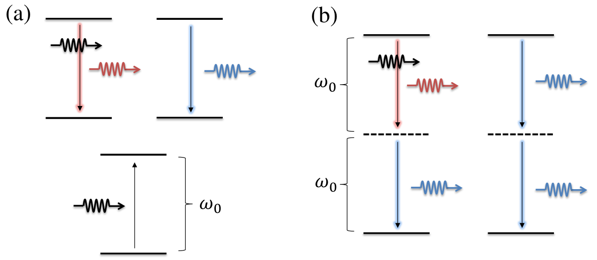
This equation was derived from first principles starting from an atom-photon Hamiltonian with two-photon interactions by Lambropoulos in which $\kappa_{\Uparrow}$ and $\kappa_{\Downarrow}$ are further related to microscopic quantities ²² 2 Equation (3.13) of Ref. Lam67 is equivalent to (13) in the Fock basis.. Here, it suffices to express them as $\kappa_{\Uparrow}=\gamma\,n_{\Uparrow}$ and $\kappa_{\Downarrow}=\gamma\,n_{\Downarrow}$ where $\gamma$ is an effective atom-photon coupling strength while $n_{\Uparrow}$ and $n_{\Downarrow}$ are the fractional atomic populations in the excited and ground states respectively. Two-photon amplifiers have been widely studied for some time Lam67; MW74; NEFE77; NZT81; BRGDH87; AGBZ90; GWMM92; Iro92; Gau03; NHO10; HNGO11; RSSHS16; MRBB18 and their output photon statistics have been intensively studied for the model of (13) and special cases of it Lam67; MW74. Already in Ref. Lam67, Lambropoulos noted that linear amplification, i.e. one-photon gain, was somehow possible with ${\cal L}_{2}$ upon setting $\kappa_{\Uparrow}=\kappa_{\Downarrow}=\gamma/2$ in (13) despite the amplifier being described by an inherently two-photon model [See Sec. V.C of Lam67. Also compare his Eqs. (5.9b)–(5.9c) with our Eqs. (5)-(6)]. To explain this he postulated that the amplification had to involve a ‘‘half noise half signal’’ process, originating from two-photon emissions whereby ‘‘the emission of one of the photons is induced and the other spontaneous’’ ³³ 3 See the main text on the last page of Ref. Lam67.. However, to the best of our knowledge, this assertion has remained unsubstantiated to date. If we are able to affirm the speculated mechanism underlying ${\cal L}_{2}$, we would not only have validated Lambropoulos’s conjecture, but will also be guided to what kind of physics prevents a phase-preserving linear amplifier from being simulable by a paramp. As we now explain, ${\cal L}_{2}$ can be understood in terms of the elementary atom-photon interactions shown in Fig. 2(b).

Attempts to understand the photon statistics of the two-photon amplifier naturally treat the density operator of the signal mode $\hat{a}$ as a central object of analysis, and thus work in the Schrödinger picture. This is a major drawback in understanding the noise mechanism because the internal modes of the amplifier noise are traced out in such a description Lam67. We are therefore motivated to work in the Heisenberg picture where the amplifier noise appears explicitly as a time-dependent operator. This will allow us to track how the noise arises at the output and arrive at Fig. 2(b).

Before we analyse ${\cal A}_{2}(t)$ in the Heisenberg picture, it is instructive to review how such an analysis works for the example of ${\cal A}_{1}(t)$. Its Heisenberg-picture equivalent for the signal $\hat{a}(t)$ can be shown to be given by CHN+19; GZ10

where $d\hat{s}(t)\equiv\hat{s}(t+dt)-\hat{s}(t)$ for arbitrary $\hat{s}(t)$. Equation (14) may be derived from a familiar model of the field interacting with a two-level atom. In this case, $\kappa_{\uparrow}$ and $\kappa_{\downarrow}$ are the effective excited-state and ground-state populations in an atomic gain medium that implements one-photon interactions. The term $d\hat{W}(t)$ is a quantum Wiener increment and represents the noise being added to the signal as it is being amplified according to (14). It is an atomic operator that is independent of the signal and has zero mean. All its higher-order moments vanish except the second-order ones given by the quantum Itô rules GZ10; Ito42; Ito44; Ito46; HP84; WM10

Since we are now working explicitly in continuous time, the input and output signals are to be identified as $\hat{a}(0)$ and $\hat{a}(t)$ respectively. Applying quantum Itô calculus, (14) can be shown to satisfy $[\hat{a}(t),\hat{a}^{\dagger}(t)]=\hat{1}$ for all $t$, as required in order to be consistent with quantum mechanics.

The advantage of (14) is that it allows us to see how the noise contributes to the amplifier output explicitly. In particular, we can extract some basic physics about the amplification of $\hat{a}$ by considering the evolution of the average photon number:

The first two terms in (17) show that population inversion in the gain medium is necessary for a positive contribution to the signal’s energy, i.e., for amplification. The third term given by $\kappa_{\uparrow}$ comes directly from the noise operator $d\hat{W}(t)$ and represents noise photons added to the signal. Furthermore, each term in (17) can be understood to correspond to an elementary atom-photon interaction (i.e., stimulated emission, absorption, or spontaneous emission) Aga13; Mil19: The first term is proportional to both the intensity of the light reaching the atom $\langle{\hat{n}(t)}\rangle$ as well as the effective atomic population of the excited state $\kappa_{\uparrow}$ and corresponds to stimulated emission. Similarly, we know that the number of absorption events in the gain medium should be proportional to $\langle{\hat{n}(t)}\rangle$ and the effective ground-state population of the atoms. This corresponds to the term $-\kappa_{\downarrow}\langle{\hat{n}(t)}\rangle$ in (17) where the negative sign indicates that absorption removes energy from the field. The only atom-photon interaction that does not depend on the signal’s energy, but only on the excited-state population of the gain medium, is spontaneous emission, and is given by the last term in (17). This highlights the well-known facts about linear amplifiers that rely on single-photon interactions: First, that stimulated emission and population inversion are essential for amplification, and second, that spontaneous emission is the physical mechanism responsible for adding noise to the signal. A summary of these processes is shown in Fig. 2(a).

The Heisenberg-picture equation for $\hat{a}$ corresponding to the two-photon amplifier of (13) is CHN+19

This is an Itô quantum stochastic differential equation Chi15; Par92; WZ65; Gou06; GC85 where $d\hat{W}(t)$ is again an atomic operator with zero mean and such that

Again, it can be shown that (Phase-preserving linear amplifiers not simulable by the parametric amplifier) preserves $[\hat{a}(t),\hat{a}^{\dagger}(t)]=\hat{1}$ for all $t$ CHN+19. The Heisenberg equation of motion for $\hat{a}$ corresponding to ${\cal L}_{2}$ may then be obtained from (Phase-preserving linear amplifiers not simulable by the parametric amplifier) by setting $\kappa_{\Uparrow}=\kappa_{\Downarrow}=\gamma/2$. This gives

Note here that (20) now carries a signal-dependent noise given by $\hat{a}^{\dagger}(t)d\hat{W}(t)\,$. This is the “half signal half noise” which Lambropoulos spoke of in Ref. Lam67. It is also referred to as multiplicative noise in random process theory Jac10; Gar09. We can now show exactly what the multiplicative noise in (20) is in terms of elementary atom-photon interactions by considering how the average photon number evolves. Using quantum Itô calculus we have,

The first term in (22) is inherited from the $\gamma\,\hat{a}(t)dt$ term in (20) and corresponds to one-photon stimulated emission as it depends on $\kappa_{\Uparrow}$ and $\langle{\hat{n}(t)}\rangle$. Since the model restricts the atoms to have only two-photon transitions, this term by itself does not complete a full atomic transition from excited to ground state with the emission of two photons. To complete the picture we must take into account for the photons from the remaining terms in (22), which are noise photons insofar as they arise from the atomic operator $d\hat{W}(t)$. In contrast to (17), there are now two types of noise photons. The first is linear in $\langle{\hat{n}(t)}\rangle$, so it corresponds to a one-photon emission that depends on the signal strength reaching the atom. The fact that it is a noise photon suggests that it came from spontaneous emission while the fact that it depends on the signal means that such a spontaneous emission is “stimulated”—conditioned on a stimulated emission having taken place just before it. The seemingly strange possibility of getting one-photon amplification in a two-photon model can now be resolved when we take the stimulated photon corresponding to the first term in (22) together with the signal-dependent noise photon to arrive at the two-photon process shown on the left of Fig. 2(b). This is the underlying mechanism responsible for linear (i.e. one-photon) amplification in a gain medium with only two-photon transitions. The remaining type of noise photon is due to the $2\gamma$ in (22) which corresponds to two-photon spontaneous emission. This is shown on the right in Fig. 2(b).

Our physical picture of the multiplicative noise in (20) thus allows us to see how it is signal dependent. It is precisely this signal-dependent noise that leads to a photon-number gain of $g^{4}$ in (6) which ultimately makes it impossible for the paramp to simulate it as shown in (11). This can be seen explicitly from (22) where the first term contributes photons at a rate $2\gamma\langle{\hat{n}(t)}\rangle$ to the signal, while the signal-dependent noise contributes another $2\gamma\langle{\hat{n}(t)}\rangle$ photons per unit time to make up a total rate of $4\gamma\langle{\hat{n}(t)}\rangle$ [which leads to the fourth power of $g$ in (6) and subsequently in (11)]. Because (20) is the simplest form of a phase-preserving linear amplifier with multiplicative noise, it may be expected that other such amplifiers with more complicated signal-dependent noise can also violate (3), as we showed with ${\cal A}_{3}(t)$ from Eq.(12).

We note that non-degenerate variants of the left picture in Fig. 2(b) (i.e. a two-photon emission with unequal transition frequencies) has been observed in experiments and are known in the literature as singly stimulated emission HGO08; NBH+10; OIKA11 (see Ref. HNGO11 and the references therein for more details). What we have done in this section on the physical properties of our counterexamples is to show that (i) multiplicative noise prevents a phase-preserving linear amplifier from being paramp simulable, and (ii) explain the physical basis of this multiplicative noise in terms of elementary atom-photon interactions.

It is also possible to interpret (20) and its associated linear amplification purely from the perspective of quantum stochastic processes. In this interpretation (20) is understood to generate linear amplification as a result of the correlations between the amplifier-added noise and the signal. This follows from the Stratonovich form of (20) which is derived in Ref. CHN+19. Such a process may in principle be realised using ion traps SMrefs.

Finally, our discussion above sheds light on how ${\cal A}_{2}$ evades the claimed proof of the universality of the paramp model in Ref. CCJP12. The authors of Ref. CCJP12 mathematically characterize a phase-preserving linear amplifier as a composition of a perfectly noiseless (and unphysical) amplifier with a noise map that restores physicality ⁴⁴ 4 See Equation (3.2) and the surrounding discussion in Ref. CCJP12.. Crucially, this added noise was taken to be signal-independent, thus excluding multiplicative noise of the kind found in ${\cal A}_{2}$ by fiat.

References

- (1) P. D. Drummond and M. Hillery, The Quantum Theory of Nonlinear Optics, (Cambridge University Press, 2014).
- (2) H.-P. Breuer and F. Petruccione, The Theory of Open Quantum Systems, (Oxford University Press, 2002).
- (3) H. J. Carmichael, Statistical Methods in Quantum Optics 1 (Second-corrected-printing), (Springer, 2002).
- (4) C. Gardiner, Stochastic Methods (Fourth edition), (Springer 2009).
- (5) K. Jacobs, Stochastic Processes for Physicists: Understanding Noisy Systems, (Cambridge University Press, 2010).
- (6) K. R. Parthasarathy, An Introduction to Quantum Stochastic Calculus, (Birkhäuser, 1992).
- (7) C. W. Gardiner and P. Zoller, Quantum Noise (Third edition), (Springer, 2010).
- (8) E. Wong and M. Zakai, Int. J. Engng. Sci. 3, 213 (1965).
- (9) J. Gough, J. Math. Phys. 47, 113509 (2006).
- (10) C. W. Gardiner and M. J. Collett, Phys. Rev. A 31, 3761 (1985).
- (11) D. Leibfried, R. Blatt, C. Monroe, and D. Wineland, Rev. Mod. Phys. 75, 281 (2003).
- (12) T. E. Lee and H. R. Sadeghpour, Phys. Rev. Lett. 111, 234101 (2013).
- (13) H. M. Wiseman and G. J. Milburn, Quantum Measurement and Control, (Cambridge University Press, 2010).
- (14) M.-H. Chiang, Quantum Stochastics, (Cambridge University Press, 2015).
- (15) C. M. Caves, J. Combes, Z. Jiang, and S. Pandey, Phys. Rev. A 86, 063802 (2012).
- (16) C. M. Caves, Phys. Rev. D 26, 1817 (1982).
- (17) M. O. Scully and M. S. Zubairy, Quantum Optics (Cambridge University Press, 1997).