Random Feedback Shift Registers, and the Limit Distribution for Largest Cycle Lengths
Abstract
For a random binary noncoalescing feedback shift register of width , with all possible feedback functions equally likely, the process of long cycle lengths, scaled by dividing by , converges in distribution to the same Poisson-Dirichlet limit as holds for random permutations in , with all possible permutations equally likely. Such behavior was conjectured by Golomb, Welch, and Goldstein in 1959.
1 Introduction
We consider feedback shift registers, linear in the eldest bit (in ), given as
| (1) |
Here
| (2) |
is an arbitrary bit Boolean function (the “feedback” or “logic”), and we will consider all possible to be equally likely. We write
and note that the map
| (3) | |||||
is a permutation on objects.
In 1959 [17], see also Chapter VII of [16], Golomb, Welch, and Goldstein suggest that the flat random permutation in , with all permutations equally likely, gives a good approximation to the cycle structure of , in the sense that the cycle structure of is close to the cycle structure of , in various aspects of distribution, such as the average length of the longest cycle. See [21], especially the section “Cellular Automata and Nonlinear Shift Registers,” which includes an anecdote that Golomb used custom hardware modules in 1956 to experiment on this conjecture, and these ran about 3 million times faster than the general purpose computer on the same problem.
We prove that the longest cycle part of this conjecture is true, and more, namely that and have the same limit distributions in the infinite-dimensional simplex , for the processes11 1 A (stochastic) process is simply a collection of random variables, or, depending on one’s point of view, the joint distribution of that collection. of long cycle lengths, scaled by . This does not answer other aspects of Golomb’s conjecture, involving the distribution of the number of cycles, or behavior of short cycles.
There are two natural ways to view the large cycles of the random permutation , which we now describe briefly. First, there is the process of largest cycle lengths: write for the length of the longest cycle of , with if the permutation has fewer than cycles, so that always , where . Write for the process of scaled cycle lengths, . Second, there is the process of cycle lengths taken in age order: pick a random -tuple, take to be the length of the cycle of containing that first -tuple, then pick a random -tuple from among those not on the first cycle, take to be the length of the cycle of containing that second -tuple, and so on. Write for the process of scaled cycle lengths in age order. For flat random permutations in place of , the limit of is called the GEM process (after Griffiths [18], Engen [15], and McCloskey [20]); it is the distribution of , where are independent and uniformly distributed in . The Poisson-Dirichlet process is where is the largest of . This construction gives the simplest way to characterize the Poisson-Dirichlet process, PD. For flat random permutations, the limit of is PD.22 2 This same Poisson-Dirichlet process also gives the distributional limit for the process of scaled bit sizes of the prime factors of an integer chosen uniformly from 1 to , as goes to infinity. Here we write PD for PD, where, in general, GEM and PD for are constructed using in place of , and the case gives the limits for the processes of sizes of largest components, in age order or strict size order, for random mappings, i.e., functions from to with all possibilities equally likely. See Section 5.1 for a review of these concepts, including more discussion of age-order and the GEM limit as used in (5). See also [3]. Formally, our result is the following:
Theorem 1.
Writing to denote convergence in distribution, we can succinctly summarize the conclusion of Theorem 1 by writing
| (4) |
We note some easy consequences of Theorem 1. Theorem 1 is equivalent to
| (5) |
with GEM distribution, by a soft argument involving size-biased permutations, originally given by [13]. By projecting onto the first coordinate33 3 Since and all have the same distribution, uniform in ., we see
| (6) |
By taking expectations, we see
| (7) |
Of course, the uniform distributional limit in (6) makes no local limit claim; it is plausible that holds uniformly in . For any fixed , the statement is false. It is true that . And for any fixed the statement is false; see [10].
We work with the de Bruijn graph , with edge set and vertex set ; edge goes from vertex to vertex . The graph is 2-in, 2-out regular, and a random feedback logic corresponds to a random resolution of all vertices; the resolution at a vertex pairs the incoming edges, and , with the outgoing edges and . The cycles of a random permutation correspond exactly to the edge-disjoint cycles in a random circuit decomposition of the Eulerian graph .
2 A Survey of the Proof of Theorem 1
In this section we survey the proof of Theorem 1 while omitting many necessary technicalities. It is hoped the reader will thus have a better notion of what is happening, and why, as s/he reads the later sections. We begin with the notion of relativisation. Suppose, as for example in the hypotheses of Theorem 1, that one has for each a probability on the permutations of a set . Let be one such permutation, and let be a -tuple of, for now, distinct elements from the domain . Picturing the permutation as a collection of disjoint cycles, one sees that by ignoring all elements of except for the , these latter are permuted among themselves. That is, starting with , traverse the cycle of containing this element: –
until after one or more steps an element is encountered. (It is possible for the first element so encountered to be , which happens when the traversed cycle contains only a single member of the -tuple .) Since the are given in a definite order, the induced permutation among these elements is readily identified with an element of , the permutations of the set . Altogether, we have a function
which we call relativisation. Here, denotes the ordered -tuples drawn from without replacement. We shall prove: Suppose that for every fixed the sequence of distributions induced on by the functions and the probability distributions tends to the uniform distribution. (For brevity, we say “ has the uniform relativisation property.”) Then the large cycle process associated with tends to Poisson-Dirichlet. The proof that the uniform relativisation property implies the Poisson-Dirichlet property appears in Section 5.3, as Lemma 4.
Henceforth we specialize to the particular sequence of interest: the sets are the binary -tuples , and assigns equal weight to each of the shift register permutations (and no weight to other permutations), where . Let denote the Cartesian product
For technical reasons we define the relativisation function on the set , see Definition (1) in Section 4.10. Nevertheless, pairs in which contains a repeated element may be safely ignored by the reader for now, and only the primary objective be kept in mind: to show that as varies over the coverage of under the relativisation function is approximately uniform.
Roughly speaking, this objective is accomplished by partitioning the set into blocks such that the restriction of to each block of the partition yields an almost uniform coverage of . The description of these blocks involves the notion of toggle. Let and be a feedback function; then the toggle of the function at the point is the function which disagrees with only at the argument :
That is, we have toggled a single bit in the truth table of . Toggling a feedback function has a predictable effect on . In particular, for , if and
and, (with ), , and
then (let the reader check by drawing a picture)
where denotes a transposition in . The blocks in our partition of arise as follows: given , we determine, in a way explained below, a subset of size ,
and define the block containing to be the different toggles , ranging over subsets of . Here, denotes function toggled at all . For the block to be well defined, it must be the case that the choice of will be the same for all as for . This necessitates the introduction of a subset , the “happy event,” see equation (42) in Section 4.8. It turns out that the happy event is almost all of , , and for the blocks are well defined. Moreover for each such block we have an ordered sequence of transpositions ( with
where . For sufficiently large, almost all such sequences of transpositions yield compositions which cover almost uniformly. (Lemma 2 in Section 4.9 proves that for all there is an such that the distribution induced on is within of uniform in total variation for all but an fraction of possible sequences.)
Let us say something about how, given , the -subset of is chosen. The pair determines segments
| (8) |
in which the length is taken to be approximately . For this length it is almost certain that not only are the initial edges distinct, but in fact all of the edges are distinct. This feature is included in the definition (42) of event . Given that acts by shifting left and bringing in one new bit on the right, each sequence (8) is equivalent to a binary sequence
of length . To be considered for membership in , an -tuple must appear in two of these binary sequences; that is, for some and some bit
One may ask as varies uniformly over what is the probability of finding such leftmost -repeats in various regions of the plane? Remarkably, such points when rescaled as constitute, in the limit with respect to total variation distance, a familiar Poisson process. Thanks to this limiting behavior we can estimate not only the probability of finding ’s which satisfy the above minimal constraint for -membership, but also the probability of finding ’s lying in a much more stringently constrained geometry, which geometry implies . Section 4 is devoted to proving these properties of and under the assumption that the probabilities in question can be approximated by a Poisson process.
We conclude our survey by saying how this last assumption is justified. We present in Section 3 an algorithm called sequential editing which begins with random binary sequences (referred to as coin-toss sequences) and edits them in such a way that the result of the editing is a set of sequences which could have been produced by choosing and forming the segments (8). Even more, the probability of obtaining a particular set of sequences is exactly the same, whether we choose and form (8), or flip coins and perform sequential editing. (This is proven in Theorem 4 of Section 3.6).
Moreover, there is a “good event” , , such that when the initial coin toss sequence belongs to the leftmost -repeats in the edited sequence appear in exactly the same locations as they do in . Since is almost all of (Theorem 3 in Section 3), the study of the -induced pairs is reduced to the study of leftmost -repeats in random sequences. This new process is by no means easily evaluated, but fortunately it is in the realm of the Chen-Stein method as presented and extended in [6]. In such a manner the above described approximation is justified.
Looking back at this survey, it appears that the components in the proof of Theorem 1 have been described almost in the reverse order that they appear in the sequel. May we wish that in the end the determined reader will understand the proof forwards and backwards.
3 Comparisons with Coin Tossing Sequences
Throughout this section these conventions will be observed: denote bits; denotes an -long sequence of bits; and denotes an -long sequence of bits. A tool used in the proof of Theorem 1 is to compare the bit sequence generated by a randomly chosen feedback logic with a coin toss sequence, denoted in this section . A bit sequence generated by a feedback logic has what we refer to as the de Bruijn property: it satisfies a recursion of the form . In a sequence with the de Bruijn property the -long words and must be followed by different bits. Of course, not every coin toss sequence has the de Bruijn property. The sequential edit, defined below, of a coin toss sequence is obtained in a left-to-right bit-by-bit manner and adheres as closely as possible to , changes being made only when forced by the desire to respect the de Bruijn property. On the other hand, the shotgun edit, also defined below, of a sequence is a naive imitation of a sequential edit. In a sense and circumstances to be made precise, by the combination of Theorems 2 and 3, with high probability, these two produce the same output.
3.1 Sequential Editing
We begin with an long bit sequence
The new bit sequence of the same length,
is produced by following two rules:
- Rule 1:
-
- Rule 2:
-
For determine bit by first asking if the feedback logic bit has been previously defined; if so, set accordingly:
otherwise, define (and remember) the feedback logic bit in such a way that and agree.
Here we give some terminology, and indexing practice. We say that the sequence is obtained from the coin toss sequence by sequential editing. Each time a has freedom – because the necessary feedback bit has not yet been set – we set the feedback bit so that ; but at any time the bit “has no choice,” we assign it the forced value. Such a time is a time of a potential edit; if it turns out (by chance) that and agree, then no actual edit has taken place; if it is forced to take equal to then an actual edit has taken place, and we label the time of this actual edit as rather than . The sequence obtained by this process always has the de Bruijn property. In terms of the de Bruijn graph with all vertices resolved, a potential edit occurs at time when , the edge from to , is going in to a vertex where , the resolution of that vertex, is already known, so that the successor edge, is determined — this is equivalent to determining , the rightmost bit of .
3.2 Shotgun Editing
Now we define a second, generally different, way to edit the coin toss sequence to produce a sequence . We call this the shotgun edit. Unlike obtained by sequential editing, the sequence obtained by shotgun editing may not have the de Bruijn property.
The symbols , , , denote intervals of integers contained in the -long interval . We use and to denote the left- and right- endpoints of the interval . A binary sequence
| (9) |
has an -long repeat at if , and the two ordered -tuples and are equal. We say that (9) has a leftmost44 4 This terminology means that the repeat cannot be extended on the left. The concept is standard in the literature, for example [1] and [7, p. 19]. -long repeat at if, in addition, either or
This given, the shotgun edit of coin toss (9) is readily defined: make a list of all the leftmost -long repeats found in (9). Let
3.3 Zero and First Generation Words
Let
be a coin toss sequence whose leftmost -tuple repeats occur at . The zero-generation words of length are simply words of the form:
A first-generation word is a zero-generation word with exactly one bit complemented, with the index of the complemented bit required to be for some :
3.4 The Good Event
We always consider to be understood, but sometimes we will not want to emphasize the role of , hence writing . Henceforth we shall always assume that is at most , since we are interested in cycle lengths for permutations on a set of size . Let
be a length coin toss sequence whose leftmost -repeats occur at . Then the good event is defined to be the conjunction of these six conditions:
- (a)
-
neither the initial -long word of the coin toss sequence, nor any of its -offs55 5 I.e., words at Hamming distance 1, hence with our two-letter alphabet, words formed by complementing a single bit. is repeated (probability of failure );
- (b)
-
all intersections of the form are empty (probability of failure );
- (c)
-
the sets are pairwise disjoint; likewise (probability of failure );
- (d)
-
no first-generation word of length equals a zero-generation word of length , or another first-generation word of length (probability of failure );
- (e)
-
for every leftmost -repeat we have
for all (probability of failure );
- (f)
-
there is no -repeat (probability of failure ).
The indicated probabilities of failure will be proven below in Theorem 3. First, though, we will prove a theorem that explains why is called the “good event.”
Theorem 2.
If the coin toss sequence
belongs to the good event , then
- Conclusion 1.
-
The sequentially edited sequence and the shotgun edited sequence agree; and
- Conclusion 2.
-
The sequentially edited sequence and the coin toss sequence have their leftmost repeats at exactly the same positions.
These conclusions, along with Theorem 3 in the next subsection, will provide substantial control of the prevalence of -tuple repeats
Proof of Conclusion 1.
Assume, to the contrary, that the and sequences differ; let be the first position of disagreement:
There are two possibilities: (1) and ; or (2) and .
Case (1). Since we have for some , and there is a leftmost -repeat in the sequence at . But for (condition(b)); and for (condition (c)). Hence for . But , so in fact the -sequence itself has an -repeat at . But the -sequence has the de Bruijn property, and so the repeat can be backed up steps to reveal
Since ,
so in fact
| (10) |
The word on the right side of the last equality is either a zero-generation or a first-generation word; either case contradicts condition (a).
Case (2). Because is a sequential edit point, (), it must be that the -long word is appearing for a second or later time, say
We must have , since no sequential editing took place at time . (The relevant bit of the feedback logic had not yet been determined.) We know that , else the -sequence contains an -repeat which, as was explained in Case (1), backs up to yield the contradictory (10). So, ; that is, and
Because is the first point at which the and sequences disagree,
| (11) |
Suppose (for the sake of a contradiction) that none of the bits appearing on either side of this last Equation (11) was edited by the shotgun process. Then we have
| (12) |
We have thus discovered an -long repeat in the coin toss sequence, but it might not be a leftmost -long repeat. So, we look left to determine the least such that either (i.e., you’ve gone “off the board”) or the run of equalities is broken:
One of these two will happen for or else the -sequence is found to contain a -repeat, contradicting assumption (f). But then we have found a leftmost -repeat in the -sequence beginning at and ; shotgun editing would consequently modify the -bit at position . Since
we have found that one of the -bits on the right side of Equation (12), namely the one whose index is , is changed by shotgun editing, contrary to our earlier supposition that none of the bits appearing on either side of the equality (11) was edited by the shotgun process.
By condition (c), every -long word in the sequence either is a zero-generation word (matches exactly the corresponding -bits) or is a first-generation word (matches the corresponding -bits with exactly one change). Thus, at least one of the -long words appearing in (11) is a first-generation word, and this contradicts condition (d). ∎
Proof of Conclusion 2.
We will make use of the and sequences being equal. Suppose we have a leftmost repeat in the coin toss sequence,
| (13) |
By condition (e), none of these bits (or in case ) can be edited by the shotgun edit. Hence, we have a leftmost -repeat at the same place in the sequence, whence also the sequence.
On the other hand, suppose we have a leftmost -repeat in the sequence,
| (14) |
and
If
then is a first-generation word of length which equals the first- or zero-generation word , which is forbidden by condition (d). So,
| (15) |
Similarly,
| (16) |
Altogether by (14),(15),(16) we have
| (17) |
If , then the last is a leftmost -repeat in the sequence, as asserted. So, to conclude, suppose for the sake of a contradiction that and that . Then we have an -long repeat
Sliding left for steps, we will encounter a leftmost -repeat in the coin toss sequence
with by condition (f). But in such a case by the definition of shotgun editing. However, for
and by (16) The supposition that and that has been contradicted, and so (17) is, indeed, a leftmost -repeat as needed. ∎
3.5 Probability
In this section we bound the probability of failure of any one of the conditions (a)–(f) appearing in Theorem 2. Let be a set of relations, each of the form or with . We assume always that has at most one relation for a given ; that is, we don’t allow both and . What is the probability that a coin toss sequence will satisfy such a set of relations? The desired probability is provided the graph associated with is cycle free. The graph we have in mind here is where is the set and is the set of pairs such that at least one (and by convention exactly one) of the relations or belongs to .
In particular, if the graph of consists of the pairs the probability is . This is quite clear if and are disjoint, since then the underlying graph has no vertex of degree 2. It is also true if and overlap, (of course ): every vertex of degree in the graph (i.e., every element of ) has one larger neighbor and one smaller neighbor. But a cycle would require at least one vertex with two smaller neighbors.
We will have frequent occasion below, in the proof of Theorem 3, to consider sets whose graphs are the union of two such -sets of pairs , and , . We begin with a lemma which shows that in many situations which arise in these proofs the probability in question is .
Lemma 1.
Let be the graph whose edges consist of two sets of pairs
and
Then is cycle free if any one of the following three conditions holds, where we assume and :
-
(i)
-
(ii)
-
(iii) , and .
Proof.
If then no vertex has two neighbors larger than it. If then no vertex has two neighbors smaller than it. In case (iii), all edges out of go to , and vice-versa. A cycle, if there is one, lies within the bipartite graph whose parts are and , and clearly the cycle must alternate edges between and types. If the cycle (of necessity even in length) uses edges of the first sort and of the second, then it has traveled in one direction and in the other. The last part of condition (iii) makes it impossible for the cycle to have returned to its starting point. ∎
Theorem 3.
Let be the good event. Then,
Proof.
We shall show that the probability that a random coin toss sequence of length fails any one of the conditions (a) through (f) in the definition of is . (More explicitly, each will be shown to fail with the probability indicated in the definition of .) We invoke the above Lemma during the proof by citing Lemma (i), Lemma (ii), and Lemma (iii).
Condition (a): [neither the initial -long word of the coin toss sequence, nor any of its -offs, is repeated.] Consider first an exact repetition. There are places where the repeated sequence can start, and by earlier remarks the probability that the second sequence repeats the first is . The same argument applies to the -offs of the initial pattern, and we conclude that the probability for condition (a) to fail is less than .
Condition (b): [all intersections are empty.] For we bound the probability of failure by using the same technique as in case (a). Suppose that . By the case of the proof we may assume disjoint from and to its right; and disjoint from and to its left. If then Lemma (i) yields the upper bound . If then Lemma (ii) yields . In the remaining case meets , meets , and meets . Thus the union is an interval, and a bound of results.
Condition (c): [the sets are pairwise disjoint; likewise .] We will prove the assertion regarding ; the other assertion is proven in an entirely similar manner. Suppose . We may assume ; otherwise Lemma (ii) implies an upper bound of . So now, both intersections and are nonempty. If any one of the four intersections is nonempty, then again the union is an interval, and we have the upper bound . So assume . Assume, for the sake of a contradiction, that . Then we have and . Without loss, let us say is left of and is left of . We have because is assumed to be a leftmost -repeat. Since is left of , ; but then , the contradiction. So, is untenable and now Lemma (iii) implies an upper bound of .
Condition (d): [no First-generation word of length equals a Zero-generation word of length , or another First-generation word of length ]. Suppose the first assertion is violated. Then we have, for some , some and some ,
| (18) |
with and with a leftmost -repeat. Let and let . If and are disjoint then using Lemma (i) the probability is bounded by . So assume they intersect, so their union is an interval. Similarly we can assume, using Lemma (ii), that and also intersect so their union is another interval. If these two intervals intersect, forming another interval, we have a probability bound of . Otherwise is empty. If then , contradicting (18). So Lemma (iii) implies for the probability. This gives an overall bound of .
Next, suppose the second assertion of (d) is violated. Then we have, for some , some and some ,
| (19) |
with , , and leftmost -repeats. As reasoned before we have , , and all empty with probability at least . It follows, from the sheer geometry of the situation, that . We may assume that , since (as proven in (c) above) the probability of failure is . We may assume that , for otherwise the union of and and is a connected interval, and then by reasoning as above a bound of results. We now have all three intersections , , and being empty; and by an obvious embellishment of Lemma (i) the probability of the remaining case is .
Condition (e): [for every leftmost -repeat we have
for all .] Say and . The probability that is not empty is , so assume . If , then, since lies entirely to the left of , . By Lemma (i) the probability of this is .
The probability that is not empty is , so assume both and are empty. The probability that is empty is, by Lemma (i), , so assume . If or is nonempty then is an interval, and the probability of this is . So, assume . If , then
an impossibility. So, and Lemma (iii) gives the bound for this final scenario.
Condition (f): [there is no -repeat.] Easily, the failure probability is at most . ∎
3.6 Coin Tossing Versus Paths in the de Bruijn Graph
Theorem 4.
Let be a bit string. Then, the probability that this string arose by the sequential editing of an long coin toss sequence is the same as the probability that it arose by choosing a logic and starting position each uniformly at random.
Proof.
Without loss of generality we assume the given string has the de Bruijn property. (Else, the two probabilities are both zero.) First, let’s compute the probability that arose by sequential editing of a -long coin toss. The probability of the coin toss yielding is . Consider , with . If is equal to for some in the range , then sequential editing says to let be what it ought to be: . In which case, it does not matter what value has. But if and has not been seen before (among -long words ending at a position greater then or equal to ), then must be equal to . (And, we remember henceforward the value of is .) Altogether, then, the probability that a length coin toss will yield a given sequence by sequential editing is where
Now let’s compute the probability that arose by choosing a starting position and logic at random. Classify each position , , as Type I or Type II. The position is Type I if and the preceding long word is appearing for the first time in the -sequence. The position is Type II otherwise: either , or the preceding long word is appearing for the second or later time. It should be clear that the probability in question is
The two probabilities just calculated agree.66 6 There are several interesting results in Maurer [19] for cycles in de Bruijn graphs; one must be careful to think about the factor in going back and forth between these estimates, and estimates for a random , corresponding to randomly resolved de Bruijn graphs. ∎
3.7 Notation for Paths Starting at Random -tuples
We now fix and use the notation to name random -tuples. Collectively, these edges of are denoted
| (20) |
Picking a random feedback , and random -tuples, independent of , is equivalent to picking one element, uniformly at random from the space
| (21) |
The choice of from determines infinite periodic sequences of edges: for to ,
| (22) |
For the sake of comparison with coin tossing, we often look at such paths only up to time (this is what motivated our terminology segment):
| (23) |
3.8 -sequential Editing
Now we will define a modification of the sequential editing process that was discussed earlier in Section 3.1. The reader should bear in mind our ultimate goal. We wish to study what happens when a feedback logic is chosen at random; different starting -tuples are chosen at random; and walks of length are generated, the first starting from and using the logic to continue for steps; the second starting from , etc. As in Section 3.1, we wish to generate these walks using coin tosses, and we would like to have an analog to Theorem 4 saying that our procedure for passing from the coin toss to the walks perfectly simulates the process of choosing a logic and starting points at random. The reader can almost certainly envision the natural way to achieve this, but we will write out the details.
The first coins are used exactly as in Section 3.1: Rule 1 is applied to the first coin tosses to yield starting point , and then Rule 2 is applied times to get the overlapping -tuples that form the first walk. Equivalently, this segment is spelled out by the de Bruijn bits , and along the way, some feedback logic bits have been defined.
Then, for the next coin tosses, for to inclusive, sequential editing is suspended; again Rule 1 is applied, to give
with no new feedback logic bits learned. Then, Rule 2 is applied for the next input bits, for to to create the second walk of length , — remembering of course those feedback logic bits that were learned during the creation of , and (most likely) learning some new feedback logic bits in the process. (It might be the case that , or that appears in the first walk, in which case, we don’t learn any new feedback logic bits.) If , we continue in a similar fashion, first suspending editing for time , during which time we learn no new feedback logic bits and we form , then returning to Rule 2 for the next bits, to fill out .
For we define
| (24) | |||||
| (25) |
as given by the above procedure.
It may, or should, seem intuitively obvious that , applied to an input uniformly chosen from , induces the same distribution on the segments of length in (22), as does a uniform pick from and iteration of from each of . We claim that the argument given in the proof of Theorem 4 can be adapted to show this.
3.9 The Good Event for -sequential Editing
There are two different ways to produce walks each of length out of a sequence of coin tosses. The first, with playing the role of , is simple sequential edit, to determine a starting -tuple , and one path corresponding to iterates of starting from . The good event, regarding this first procedure, is really . We can then cut the path of length to produce paths of length ; see (31) to see the natural notation associated with such cutting. The second procedure is is to apply , defined in the previous section, to produce a -tuple of starting edges, , and segments of length , as in (23). The good event, regarding this second procedure, to be called , is designed so that the two procedures agree. We simply take all of the demands of the good event for simple editing on coins, and throw in additional requirements to ensure the suspensions of editing involved in the definition of . Informally, these additional requirements are that every tuple which appears at some time involved in suspension occurs at no other time in the coin toss sequence. Formally, given , the bad event is given by
| (26) |
where the event if , and otherwise
and the good event is then
| (27) |
Since a word of length has neighbors at Hamming distance 1 or less, for , so that , for the sake of extending Theorem 3.
We now consider the following to have been proved; it is a single theorem, to give the extensions of Theorems 2 and 3 and 4, appropriate to sequential editing. Note that in the final conclusion of Theorem 5 we treat as fixed while , so that and are of the same order, and we take the assumption so that the three terms in the bound from Theorem 3 are covered by a single term.
Theorem 5.
- (i)
The procedure , applied to a coin toss sequence
chosen uniformly at random from , yields segments of length , with exactly the same distribution as obtained by a random feedback logic and starting -tuples, .
- (ii)
The good event , defined by (27) — which ultimately involves conditions (a) through (f) from Section 3.4, applied with in the role of , is such that for every outcome in , the bit sequence (and the equivalent sequence of overlapping -tuples, ) formed by single sequential edit agrees with the shotgun edit of the coins, and leftmost -tuple repeats have the same locations in and in .
- (iii)
Also, on the good event , the segments of length , produced by and notated as in (23) match exactly with , produced by cutting the output of the single sequential edit of coins.
- (iv)
Finally, if with fixed, then .
We summarize: there is an exact operation, sequential editing of coin tosses, which achieves the exact distribution of , as induced by a uniform choice of from its possible values, followed by starting at and taking iterates of the permutation . There is a good event , with provided that , for which the sequential edit agrees with the shotgun edit, and iff the coins have a leftmost -tuple repeat at . This sequential edit can be used with in place of , to create one long segment; there is the corresponding good event , . There is a second, distinct operation, , for editing coin tosses, to yield the exact distribution of segments of length under a single logic and starting -tuples, ; that is, the distribution of as induced by a uniform choice of from its possible values. And there is a corresponding good event , with
formed by adding the constraint that or implies that there is not an tuple repeat at . On the event , the -sequential edit agrees exactly with the cutting of .
3.10 A Cutting Example
We now illustrate some of the concepts just introduced, with an example and with Figures 1-4. Take . So, to generate segments of length , we start with coin tosses, used to generate one segment of length . When we have in mind a single segment of length , we will use a single subscript to label the edges, so that with , the segment is a list of edges
| (28) |
The coin tosses, indexed from to , are labeled , the de Bruijn bits formed by sequential edit are labeled , and the bits formed by shotgun edit are labeled . On the good event , we will have for all . The vertex is the - tuple of bits starting with , the edge is the -tuple of bits starting with , and edge at time goes from vertex to :
We also view the segment in (28) as a list of vertices, or as a list of bits, and abuse notation by writing equality, so that
| (29) |
| (30) |
Since we are particularly interested in leftmost -tuple repeats, we shall suppose that we are in the good event , and the leftmost -tuple repeats in the coin-toss sequence are at (56,153), (120,260), and (135,175). Thanks to occurring, we know that all 291 edges to are distinct, and the only vertex repetitions are , and . One way of indicating where these vertex repeats occur is to draw some auxiliary lines pointing to the locations, as in Figure 1. Figure 2 gives a two-dimensional (“spatial”) view of the same situation.
When we cut the single long segment in (28) into segments, we use two indices; the first runs from 1 to , and the second runs from 0 to . Including the relation with (28), for Example 1, but with the labels overloaded — since they also appear on the left side, naming the starting edges for the segments — this will give
The same segments of length , presented as lists of vertices (which here are 9-tuples) are notated as
| (31) |
Collectively, these segments are given by a deterministic function of , where names all starting points.
3.11 Coloring
Imagine the segments of length as pieces of (directed) yarn, with different “primary” colors. Vertices that appear only once get the primary color of the segment they come from; vertices that appear twice on the same segment might be visualized as having a more saturated version of the primary color of that segment. The interesting case occurs when a vertex appears on two different segments; such a vertex, call it , gets each of two primary colors — and its secondary color shows which two segments this vertex lies on; for example imagine that the two strands are red and yellow, so that is colored orange. Figure 3 on page 3 and Figure 4 illustrate this coloring.
4 Toggling
To toggle a logic at a vertex is simply to get a new from the old, by changing the value at . This is called a “cross-join step”, and is studied extensively in the context of cycle joining algorithms to create a full cycle logic. Our interest in toggling is different: we have segments induced by a logic and starting -tuples, , and we want to choose different “toggle points” in the role of , to get a nice family of related logics. All this is done in the interest of showing that the chance that and lie on the same cycle of is approximately one-half, for large , and more generally, that the chance all lie on the same cycle is approximately , and even more, that the permutation , relativized to , is approximately uniformly distributed over all permutations. This introductory paragraph is intentionally short and vague; the full details use all of Sections 3 – 6. Section 4.1 gives a longer attempt at introduction, including Figure 5, showing the huge collection of candidate toggle vertices, using colors to help visualize the segments of interest.
4.1 Big Picture Perspective: Colored Segments, Toggle Points
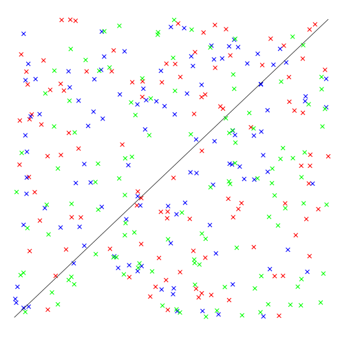
We will have segments each of length . The expected number of leftmost -tuple repeats within a single segment is about . The expected number of repeats between two different given segments is about , so the expected number of repeats between two different segments, combined over all choices for which two segments, is about . This is a huge number of repeats (each based on one vertex having a secondary coloring), and we intend to find such repeats, say at in narrowly constrained spatial positions. The goal is to show that, with high probability, for all choices of how to change by toggling the values of for , the same vertices will be picked out by the narrow two-dimensional spatial constraints.
In this section we present further figures intended to assist the reader’s intuition. We also give an algorithm which for a given logic and starting edges finds vertices , …,. These points—we call them toggle points—give rise to a family of functions. We also define (in Section 4.10) a process called relativisation which associates with in a permutation in , being fixed and . It will be shown that as varies over the functions in a “toggle class”, the resulting cover almost uniformly. In Section 5, it will be shown that this uniform coverage of (for each fixed ) is a sufficient condition to prove Theorem 1.
A critical issue is that the algorithm for choosing the toggle points must be such that, if the feedback is replaced by any one of the functions in the toggle class, the algorithm would find the same toggle points and the same class.77 7 Consider the simplest situation, and , where one is trying to prove (7) by showing that lie on the same cycle) is approximately one half. Knowing that the segments starting from and have high probability of reaching a common vertex , and that performing a cross-join step by toggling the logic at this , to get a new logic , changes whether or not and lie on the same cycle, one might consider the proof complete. The fallacy is that this procedure does not pair up with , i.e., it need not be the case that , because the procedure used to find (from , given ) might find a different when applied to . Overcoming this fallacy entails the study of displacements, starting in Sections 4.2 – 4.4. However this is not necessarily the case and the probability of success for the algorithm must be estimated; this leads to the definition of an event .

4.2 Toggling: The Case and .
We show what can happen when we toggle one bit of a logic . We have two segments of length , which share a vertex . Toggling changes the value of , only at , and gives a new logic . Suppose that the segments under were red and yellow, and that appears at position on the red segment, and position on the yellow segment. Overall, this repeat has spatial location , and color orange. Exactly one such repeat was visualized in Figures 2 and 3; it occurred with . The displacement is — we have a preferred sequence of colors, (derived from the rainbow ROY G. BIV) where red comes before yellow — hence the displacement is 3, rather than , in this example.
4.3 Picking the “Earliest” Toggle with a Small Displacement
Consider the case where we have segments, and want to find a single vertex via a recipe which, when applied to the segments under the toggled logic , still picks out the same vertex. A good recipe involves naming a small bound on the absolute displacement (thus staying close to the “diagonal”), and then picking the “earliest” pair that satisfies the displacement bound. This was the key to overcoming the “fallacy” described in Footnote 7.
The specific choice of how to define earliest is somewhat arbitrary; we will take smallest as the first criterion for earliest, with ties to be broken according to smallest value of — given that , this is equivalent to taking smallest absolute displacement for the tie-break criterion. For use in the case of colors and color pairs , break further ties according to and then .
The logic , with value at complemented, gives a new logic , so that , while . It is possible that changing the logic bit at , will cause an earlier pair to become available as the location of a match between the two segments; so that the recipe for picking the earliest small displacement match, applied to , picks out a different vertex instead of . In this case, the word toggle is very misleading: the overall operation (find , then complement the logic at that vertex) is not an involution. Our program is to specify a displacement bound that varies with , in such a way that 1) with high probability, at least one small displacement match can be found, and 2) with high probability, the vertex for the earliest small displacement match is the same in the logic at the vertex selected for . The example in Figure 8, viewed with any , illustrates what might go wrong with respect to 2).
Recall, from Section 3, that is the length of our segments. To get high probability in 1), a necessary and sufficient condition is that
| (32) |
To get high probability in 2), a necessary and sufficient condition is that
| (33) |
The argument that (33) suffices is somewhat delicate, akin to a stopping time argument; it is easier to prove — see (37) — that a sufficient condition is that
| (34) |
and then it will be easy to arrange for situations corresponding to pairs satisfying both (32) and (34).
4.4 Displacements Caused by Toggles
Suppose we have colors, as shown in Figure 9. There are three segments of length , with respect to . The segment with respect to , starting with , colored red, has in position 6 and in position 35 — so the red segment, of length 90, is divided into an initial red path of length 6, followed by a red path of length 29, followed by a red path of length 55.
The segment starting with , colored yellow, has in position 3, and in position 75, hence it is divided into yellow paths of lengths 3, 72, 15, in that order.
The segment starting with , colored blue, has in position 37, and in position 71, hence it is divided into blue paths of lengths 37, 34, 19, in that order.
Next, consider , toggled at . Its segment starting from has length 6 red followed by length (72+15)=87, for a total length of 93. Its segment starting from has length 3 yellow, followed by length (29+55)=84, for a total length of 87. The segment starting from is still length 90, all blue. More importantly, has moved from position 35 on to position 32 on , and has moved from position 75 on to position 78 on , so these have new positions under , i.e., have been displaced.
Now consider the full effect of changing from to , by toggling the logic at the bit which appeared at positions , with , for the red and yellow segments: every red vertex later than 6 gets displaced by , and every yellow vertex later than 3 gets displaced by . If a match occurs at in the segments, and the colors involved are red, and some color, call it , with not equal to yellow, then:
- •
Case 1. Color comes after red, in the list of colors: the ordered color pair is (red,. The index belongs to a red vertex in position under the logic , and this vertex has position under the logic . So the point at moves to position .88 8 More formally, the point at , labeled by the pair of colors (,red), in the colored-spatial process of indicators of matches between segments under , corresponds to a point at in the colored-spatial process for .
- •
Case 2. Color comes before red, in the list of colors; the color pair is red). The index belongs to a red vertex, in position under the logic , but in position under the logic . So the point at moves to position .
If there is an orange match at for the segments, with and , this match will move to .
Similarly, a match between yellow, and some not equal to red, occurring at under the logic , moves to or under the logic , according to whether comes after or before yellow, in the list of all colors.
This effect can be seen in Figure 9: the orange dot is at (6,3) with displacement , the purple dot occurs at (35,37) under , but at (32,37) under and .
More cases can be seen in Figure 10.
4.5 The Natural Scale: by for length, by for area
One gets an intuitive grasp of the process of spatial locations of places where two segments of different colors share a vertex, by looking at a picture such as that in Figure 6 — even though the axes are unlabeled.
One view would be that the square is by , with , i.e., about 1.3 million by 1.3 million. The other natural view is that the square is about by , i.e., about 10.556 by 10.556, with area 111.43.
The latter point of view is natural, since at each , for each color pair , , with to allow a small discrepancy for the failure of the good event, an arrival99 9 This jargon comes from queuing theory and Poisson arrival processes; we say there is an arrival at if the indicator indexed by takes the value 1, here indicating that there is an -tuple repeat. at in those colors) and there is a leftmost -tuple repeat at a specific location1010 10 The precise location doesn’t matter, but, using Section 3.10, the location is where and . in the coin tossing sequence). Hence, scaling length by , so that area is scaled by , leads to
The picture in Figure 6, viewed as occurring on a 10.556 by 10.556 square, closely resembles a (standard, rate ) two-dimensional Poisson process, in each secondary color pair. And overall, ignoring color, the picture resembles the rate Poisson process on the by square.
There are additional requirements for the Poisson process, beyond having intensity . Namely, probabilistic independence for the counts in disjoint regions. We do have a good Poisson process approximation, for a combination of two reasons. First, the good event from Theorem 5 gives a high-probability coupling (since entails ) between coin tossing and the de Bruijn segments of length . Second, the Chen-Stein method, Theorem 3 of [6], gives a total-variation distance upper bound (tending to zero since entails ) between the process of indicators of leftmost -tuple repeats for coin tossing, and a process with the same intensity, but mutually independent coordinates.
We get our intuition from the Poisson process. But for our proofs, we will work directly with the discrete, dependent processes.
4.6 Controlled Regions for Successive Potential Toggle Vertices
4.6.1 Quick Motivation for the Geometric Progression
We will construct choice functions in (40), based on regions, defined in (36), which in turn are based on a geometric progression in (35). Here we give some motivation for this elaborate construction.
If we search for a single toggle point, in a thin and long rectangle along the diagonal, , then, in the natural scale of Section 4.5, (and ignoring factors of related to the 45 degree rotation, and of 2 for ), the rectangle is by . Condition (32) can be interpreted as meaning that the (natural scale) area, , tends to infinity — so that with high probability, matches can be found in this rectangle, and condition (33) can similarly be interpreted as meaning that , so that no matches will be found in the two-dimensional set, of area on the order of , of points within distance of the chosen location .
Now in choosing toggle points, displacements caused by earlier toggles might change the search result, and we wish to make this unlikely. In more detail: as seen in Section 4.4, toggling a logic at a vertex which appears on two different colors, at times with causes displacements in the time indices of vertices occurring later on those segments, by amounts up to . Our potential toggle points, , are controlled so that on any segment, is preceded by toggle points from among the . If the displacement caused by toggling at is at most , then in choosing , the accumulated displacements from previous toggles is at most . By taking the in geometric progression, with large ratio , this accumulated displacement in the search for is at most order of . The rectangle where we search for is thin and long, by ; the length of its boundary is order of , so the area involved in points at a distance at most from the boundary is order of . Hence with high probability, displaced indices have no effect.
4.6.2 The Search Regions
We divide the time interval into equal length pieces. On the earliest piece, with times in [0,t/m], we demand that we can find a match with very very very small, but no upper bound on other than . In the natural scale of Section 4.5 we are searching for matches in a very very very thin and very very long rectangle surrounding the diagonal line ; this rectangle has a large area. On the second piece, with times in , we relax the notion of thin, expanding by a large factor , relax the notion of long, dividing by the factor , thus keeping the area constant. We continue this pair of geometric progressions, so the th region is a thin long rectangle — but still with the same area.
Here is a concrete way to accomplish the above, together with and with fixed. Let
The last condition should be understood as “in the natural scale from Section 4.5, the by rectangle is by , and length for the discrete and corresponds to length ”. Let
and, ignoring the factors of involved in the 45 degree rotation, take the thin long rectangles to have shapes
| by | |||||
| by | (35) | ||||
| by |
Indexing by to , the th rectangle is by on the natural scale. Directly in terms of the discrete and , we define
| and | (36) | ||||
so one checks that 1) as increases by 1, the thinness constraint relaxes by a factor of , while the width constraint becomes more severe by a factor of , so the area stays constant, 2) the first region, with , allows , and 3) the last region, with , has as .
Consider the possibility discussed in Section 4.3, where a toggle at a vertex appearing in two differently colored segment enables a match within a single segment to become, after the toggle, an earlier match between two different segments. For each to , with the in (34) given by , the condition in (34) is indeed satisfied by our specific choice in (35). On the natural scale, and ignoring rotation, we are searching for a match in a by rectangle, thin and long, with and area . The condition (34), on the natural scale, means that . It implies that, with high probability, we do not find a match between two differently colored segments (at in the rectangle, with ,) and simultaneously a nearby match within a single segment. Here, nearby means with both indices within distance from or . Now, the by rectangle can be covered by squares, each square of size by , and with each successive square being a translate, by , of the previous square. Ignoring constant factors,1111 11 such as — for the intensity of arrivals in the superimposed process marking matches between two different colors or both within the same color, and 16 — since a by square has area the expected number of arrivals in one square is order of , and the chance of two or more arrivals in that one square is order of Thus the expected number of squares with two or more arrivals is order of
| (37) |
4.7 Definition of the Choice Functions
Write for the set of vertices in , and write “null” for a special value, not in , used to encode “undefined”. Recall that we write for the starting -tuples for segments, and for the space in which we make a uniform choice of logic and starting edges. Also recall our notation (31) for vertices along the segments. Note that we have both segments and colors; these are different concepts, and ultimately, colors will be labeled according to the segment labels under — but on the soon to be defined “happy” event , finding on two different segments of will be equivalent to finding on two different colors. To keep track of the colors, let
| (38) |
For to , we define
| (40) |
where the value is if the set of candidates is empty, and otherwise, picking the first in , is the vertex with . To be very careful, the order for first is the lex-first order on .
4.8 The Happy Event
We now describe a subset of , and refer to this subset as the happy event . One requirement for is that, for to , each of the values . Starting with such an , the choice functions pick out a set of distinct vertices; call them , and name the set, — we will use this notation in (42) below.
Given a set of vertices, , we denote the logic toggled at the vertices in as , defined by
| (41) |
We define as follows:
| (42) |
Informally, is in the happy event iff the segments involve no -repeats, and the choice recipes find potential toggle vertices, and all cousins , formed by toggling at a subset of those vertices, give rise to the same .
The definition above creates an equivalence relation on , in which all classes have size , and all share the same sequence . Using the calculations given in Section 4.6.1 one may show that for fixed , ; that it, that as .
4.9 Definition and Likelihood of an -good Schedule
Given , view , defined by (38) as an alphabet of size
A schedule of length is a word . Given a schedule of length , and coin tosses , for to define permutations in by
and let be the product, with applied first,
| (43) |
Write for an arbitrary permutation in , and let
be the conditional probability of getting for the value of , given the schedule — these are values of the form with in . The total variation distance to the uniform distribution on is
Given , a schedule is -good if .
Lemma 2.
Given , and , there exists such that, for a random schedule of length , with all equally likely,
| (44) |
Proof.
There is a well-known bijection between and the set : given with , take
| (45) |
where denotes the transposition if , and the identity map otherwise. (The corresponding algorithm, to generate uniformly distributed random permutations, is known as the “Fisher-Yates shuffle” or “Knuth shuffle”.)
Now consider the particular word of length over the alphabet defined in (38), given by
If we had and the schedule is , then , because for each in (45), one assignment of the coin values yields , via the coins for the genuine transpositions among the on the right side of (45) being heads, and all others coins being tails. When the word appears times inside a long word , we have, using a standard result,
For historical interest, we note that similar results are in [11, Thm. 1, p. 23]; see also [12]. In a very long random word , the number of occurrences of is random, with mean and variance roughly , so a sufficiently large guarantees that is sufficiently large, with high probability. ∎
4.10 Relativized Permutations
We will define “ relativized to ” to be a specific permutation in , where denotes the set of all permutations on . For use in Lemma 4, we need to allow for the possibility that are not distinct -tuples.
Definition 1.
Let be a permutation on a finite set , and let . In case are all distinct, write the full cycle notation for , erase all symbols not in , and then relabel as . This yields the cycle notation for a permutation , and we call “ relativized to ”. In case , edit the list by deleting repeats, from left to right, to get a new list , with no repeats. Now we take “ relativized to ” to be .
On the happy event from (42), consider an equivalence class . We want to name a canonical choice of class leader, and since all elements in the class share the same , and differ only in the values of the at those vertices, the natural choice of leader is where
Finally, we can say what colors are: for to , the vertices along have color . Among the various in the equivalence class , except for the case , at least some of the segments start with one color and end with another.
The schedule corresponding to the equivalence class is the word where where and appears on colors and , that is, is a vertex of both and . We visualize1212 12 This is a only a visualization, and not a technical definition. Imagine strands of (directed) yarn, of different colors. They are all tangled up, but the start and end of each strand protrude from the tangle, so one has protruding ends (one male, one female, in each color). One only knows that inside the tangle, there are instances of two different colored yarns being cut, and at each of these , both strands may be spliced back together in their original (no color change) form, or else they may be cross-joined. as meaning that the strands of colors and are cut (at ) and glued together to create a color jump, as in Figures 8 and 9.
For to , write the final edge of , so that, under the logic , is a directed path (in color ) from its female end to its male end . Note that being in implies that the starting edges are distinct, and the final edges are distinct.
It is clear — from the relative timing of the appearances of the along the segments — that under the logic , is a directed path from its female end to its male end , where is the permutation in given by
| (46) |
compare with (43).
Take the usual notation from Hall-style matching theory, and abbreviate the female ends as and the male ends as . Then induces the matching from to with . Now the paths under starting from the male ends must eventually arrive at female ends . Define the return matching by if the path starting from the male end first arrives at the female end . This return matching is the same under all logics with .
5 Sampling with Starts, to Prove Poisson-Dirichlet Convergence
5.1 Background, and Notation, for Flat Random Permutations
An overall reference for the following material and history is [3]. For a random permutation in , with all possible permutations equally likely, for j=1,2,…, let
with if the permutation has fewer than cycles, so that always . The notation means that we consider the two notations equivalent, so that we can use either, depending on whether or not we wish to emphasize the parameter . Write
| (48) |
so that . We use notation analogous to the above, systematically: boldface gives a process, and overline specifies normalizing, so that the sum of the components is 1.
This paragraph, summarizing the convoluted history of the limit distribution for the length of the longest cycle, begins with Dickman’s 1930 study of the largest prime factor of a random integer. Dickman proved that for each fixed , , where counts the -smooth integers from 1 to . The function is characterized by for , for , and for all , . In modern language, writing for the largest prime factor of an random integer chosen from 1 to , Dickman’s result is that
| (49) |
Later work by Goncharov (1944) and Shepp and Lloyd (1966) showed the corresponding result for random permutations, that for every fixed , . In modern language this is
| (50) |
The random variable appearing in (49) and (50) is the first coordinate of the Poisson-Dirichlet process; the second coordinate corresponds to the second largest prime factor, or second largest cycle length, and so on. For primes, the joint limit was proved by Billingsley (1972) [9], and for permutations, the joint limit was discussed by Vershik and Shmidt (1977) and Kingman (1977). In these early studies, the Poisson-Dirichlet process appears as the limit, but not in a form easily recognizable as either (54) or (55). A fun exercise for the reader would be to prove that the distribution of , as given by the cumulative distribution function in (49), together with the integral equation characterizing , is the same as the distribution of as given by its density, which is the special case of (54). See [2] for more on the Poisson-Dirichlet in relation to prime factorizations, and [4] for more on the Poisson-Dirichlet in relation to flat random permutations.
Returning to the process of longest cycle lengths in (48), the joint distribution is most easily understood by taking the cycles in “age order”. Let
| (51) |
Our notation convention has already told the reader that , and that . Here, the notion of age comes from canonical cycle notation: 1 is written as the start of the first (eldest) cycle, whose length is , then the smallest not on this first cycle is the start of the second cycle, whose length is , and so on — with if the permutation has fewer than cycles.1313 13 In contrast with permutations on , similar to (51), where age order comes from the canonical cycle notation, for shift-register permutations , the oldest cycle is not the cycle containing the lex-first -tuple, . In fact, in a random FSR, the cycle starting from has exactly a one-half chance to have length 1. For permutations of a set lacking exchangeability, such as , the notion of age order requires auxiliary randomization: the oldest cycle is picked out by a random tuple; conditional on this cycle, with length , choose an tuple uniformly at random from the remaining -tuples not on the first cycle, to pick out the second oldest cycle, whose length is , and so on. It is easy to see that is uniformly distributed in , and for each , if there are at least cycles, then
This very easily leads to a description of the limit proportions: with independent, uniformly distributed in (0,1),
| (52) |
We write to denote convergence in distribution, and we note that , where denotes equality in distribution. The distribution of the process on the right side of (52) is named GEM, after Griffiths [18], Engen [15], and McCloskey [20]; its construction is popularly referred to as “stick breaking” although stick breaking in general allows to take any distribution on (0,1), not just the uniform.
Convergence of processes, such as (52) and (56), and our Theorem 1 and Lemmas 3 and 4, are instances of convergence for stochastic processes with values in , with the usual compact-open topology, and as such, convergence of processes is equivalent to convergence to the finite-dimensional-distributions, of the first coordinates, for each .
Define
The (usual subspace) topology on is the same as the metric topology from the distance,
| (53) |
We write RANK for the function on which sorts, with largest first. An example shows some of the subtlety of the preceeding considerations: let be the standard basis vector — all zeros apart from a 1 in the coordinate, and let be the all zeros vector. Note that , and in the larger space , . But for , and the sequence does not converge in . The closure of is the compact set , and RANK is also defined1414 14 RANK is not defined on — for example does not have a largest coordinate. on ; note that , and our example shows that RANK is not continuous on . Donnelly and Joyce, [13, Proposition 4], proved that RANK is continuous on , observing that “…in parts of the literature some of these results seem already to have been assumed.”
By definition, a random is the Poisson-Dirichlet process, or has the Poisson-Dirichlet distribution1515 15 This PD is PD(1); mathematical geneticists work with a family of distributions, PD(), indexed by ., PD, if for each , the joint density of the first coordinates is given by
| (54) |
on the region and , and zero elsewhere. The Poisson-Dirchlet process may be constructed from the GEM process, which appeared on the right side of (52), by sorting, with
| (55) |
For the process of largest cycle lengths in a random permutation, (48), the combination of the easy-to-see limit (52), and the continuity of RANK, and the characterization (55) of the Poisson-Dirichlet distribution, proves that as ,
| (56) |
Our goal is to derive a new tool for proving the same PD convergence as in (56), but for non uniform permutations, such as those arising from a random FSR. It might benefit the reader to jump ahead a little, and read the statement of Lemma 4, and then the more technical Lemma 3, which has the meat of the argument used to prove Lemma 4. We have stated Lemma 3 in a fairly general form, hoping that it may be useful in the context of other combinatorial structures, and perhaps with limits other than the Poisson-Dirichlet.
5.2 The Partition Sampling Lemma
Lemma 3.
First, suppose that for each along a sequence of tending to we have a random set partition on . Let be the size of the -th largest block of , with for greater than the number of blocks of , so that . Let and let .
Next, for each , take an ordered sample of size , with replacement, from , with all possible outcomes equally likely. Such a sample picks out an ordered by first appearance list of blocks of , say , with . Let be the number of elements of the -sample landing in the block , with for , so that . Let .
Finally, let be any random element of , with , and let be any random elements of for which , and such that has
| (57) |
Then, if for each fixed , as , we have
| (58) |
it follows that
Proof.
Here is an outline of our proof. We begin with an analysis of “sampling using probes”, leading to (61), which gets coordinatewise nearness, with exceptional probability O(, uniformly over set partitions, which are indexed by . This is the crux of our proof; the remainder is similar to Donnelly and Joyce, [13, Proposition 4], on the continuity of RANK. For an overview, writing whp to mean “with high probability”, and to mean “approximately equals, in ”:
Write the blocks of as , listed in nonincreasing order of size, so that . Write , so that is a random probability distribution on the positive integers. Let be the number of elements of the -sample in ; the lists and represent the same multiset, apart from rearrangement, so that
| (59) |
Write , and , so that and .
Conditional on the value of , the joint distribution of is exactly Multinomial. We want to establish a form of uniformity for the convergence of to . The first step is to recall the usual proof that for Binomial sampling, with a sample of size and true parameter , the sample mean converges to the true parameter — because the proof provides a quantitative bound. Specifically, Chebyshev’s inequality gets used, with
| (60) | |||||
In particular, conditional on any value for , for , with in the role of for (60),
Hence, taking expectation to remove the conditioning on , and then using to analyze the union bound, we have a good event (proximity in ) whose complement
| (61) |
For , write for the sum of the largest coordinates of . Obviously
| (62) |
Let be given, and fixed for the remainder of this proof.
Let
| (63) |
the set of points in where some set of coordinates sums to more than . Note that is invariant under permutations of the coordinates, including RANK. Since , and from (57) is a random element of , there exists , depending on the distribution of , such that
| (64) |
fix such a value for . [When used in Lemma 4, where the distribution of is Poisson-Dirichlet, (55) can be used to show that the minimal such is asympotically .]
Using the hypothesis (57), and observing that is an open set, (the open set part of the Portmanteau Theorem on weak convergence implies that) we can pick and fix a finite such that for all ,
| (65) |
Using the hypothesis (57) again, we can pick and fix a finite such that for each , there exists a coupling (see Dudley [14], Real Analysis and Probability, Corollary 11.6.4) such that the distance has
| (66) |
Next, intending to use (61) with used in the role of , the upper bound is . To have this upper bound be at most , and also be able to apply (66), we take to be the maximum of and the ceiling of .
The value has been fixed, in the previous paragraph. Now, the convergence in hypothesis (58) involves the topologically discrete space , so the distributional convergence can be metrized by the total variation distance, hence there exists a finite such that for all , the total variation distance between distributions is at most , and there exists a coupling with
Of course this same coupling and exceptional event yields , and using also (65),
Next, observe that and from (61) with imply that, each of the indices for has , so the sum of those coordinates of is at least (as observed in (62))), and the sum of the other (outside the chosen ) coordinates of is at most , while the sum of the other (outside the chosen ) coordinates of is at most . Hence, the distance is at most , accounted for by , from the with among the chosen , plus using on the other coordinates, outside the chosen . This result was that . Now by construction, but due to sampling noise, maybe . However, since RANK is a contraction, we have .
Putting it all together, for any , the union of the exceptional events from (61) ( near , coordinatewise, with ), from (66) ( near ), and from (67) ( equals , in ) has probability at most , and outside this exceptional event, is at most away from , which in turn is at most away from . In summary, there are couplings so that
∎
5.3 The Permutation Version of the Sampling Lemma
Lemma 4.
Suppose that for a sequence of tending to we have a random permutation on . Let be the size of the -th largest cycle of , with for greater than the number of cycles of , so that .
Given , take an ordered sample of size , with replacement, from , that is, with all possible outcomes equally likely. Let be relativized to , as defined at the start of Section 4.10.
Now suppose that, for each fixed ,
| (68) |
Proof.
Take the processes of cycle lengths, in age order, as given by (51), for uniform random permutations in , to serve as the random elements in the hypotheses (57) and (58) of Lemma 3. This requires using the Poisson-Dirichlet distribution, for in (57).
Fix . Then (68) holding for each implies that the distribution of is close, in total variation distance, to the uniform distribution on . On the event, of probability , that the -sample with replacement from the population has distinct elements, the counts from Lemma 3 agree exactly with the cycle lengths in . Hence hypothesis (68) implies the hypothesis (58).
∎
6 Putting it All Together: The Proof of Theorem 1
We now have established all the ingredients needed for our proof of Theorem 1. First, the conclusion (4) of Theorem 1 is exactly the conclusion (69) from Lemma 4.1616 16 There is a small shift of notation; in Section 5 we had to deal with both FSR permutations and flat random permutations. So in Section 5, instead of for the process of largest FSR cycles lengths, names the process of largest cycle lengths for an FSR permutation, and names the corresponding process for flat random permutations. To prove Theorem 1, it only remains to establish that the random FSR model (1) satisfies the hypothesis (68) of Lemma 4.
Fix for use in (68). The uniform choice of determines and the random sample — for convenience in Lemma 4 we labeled the set with the integers 1,2,. Let an arbitrary be given. Fix as per Lemma 2, so that with high probability, a random schedule of length over the alphabet of size is -good.
We will take , recalling that . By Theorem 5, for sufficiently large , on a good event of probability at least , the two-dimensional process of indicators of vertex repeats, in , agrees with the two-dimensional process of indicators of leftmost -tuple repeats for coin tossing; and cutting, to produce and segments, causes no unwanted side effects. Then, by the Chen-Stein method as given by Theorem 3 of [6] (with a survey of applications to sequence repeats given by Section 5 of [7], and details for the sequence repeats problem given in (39)–(40) of [8]), for sufficiently large the total variation distance between and is at most , where has the same marginals as , but all coordinates mutually independent. Combined, the total variation distance between and is arbitrarily small, at most .
The indicator of the happy event is a functional of the process , so we can approximate , with an additive error of at most , by evaluating the same functional, applied to . The required estimates for this independent process are routine, via computations of the expected number of arrivals in various regions as in Section 4,1717 17 These arguments take two forms: 1) if the expected number of arrivals is small, specifically, less than , then the probability of (no arrivals) is large, specifically, greater than , and 2) if the expected number of arrivals is sufficiently large, specifically, some , and the indicators of arrivals are mutually independent, then the probability of (no arrivals) is small, specifically, at most . It is precisely the role of the Chen-Stein method to provide the required independence. and we have already provided most of the details, in discussing (32) and (34). Additionally, one must check that the schedule resulting from use of (40) is close, in total variation distance, to the flat random choice in the hypothesis of Lemma 2; we omit the relatively easy details.
To summarize, we picked for use in Lemma 4, then fixed an arbitrary , then picked via Lemma 2.1818 18 In a sense, Lemma 4 encapsulates a relation between an arbitrary , and , hiding the full program: given to govern being close with high probability, pick a single large enough that the -sampled-and-relativized permutation being close to uniform in would imply that the large cycle process for FSR permutation is close to the PD, then pick a single to work for this and , then finally pick , the notion of sufficiently large , to work for this and . The briefest summary is: given , pick , then , then . For large , the process of vertex repeats among the segments of length is controlled, via comparison of , showing that most lie in , and furthermore, the event , that the chosen potential toggle vertices pick out a -good schedule, has . (Attributing to , to , and to .) Section 4.9 shows that, on , the settings of at its toggle vertices induce a nearly flat random matching between segment starts and ends, and (47) in Section 4.10 lifts this to show that relativized to is a nearly flat random permutation in . Thus the combination of Section 4.9 and 4.10 shows that, on , on each equivalence class , the total variation distance to the uniform distribution on is at most . Hence, averaging over the classes in , and allowing distance 1 for the at most of probability mass outside of , we get that for our fixed , for arbitrary , for all sufficiently large , uniform, which establishes (68). This completes the proof.
7 Acknowledgments
We would like to acknowledge numerous helpful discussions with Danny Goldstein, Max Hankins and Jay-C Reyes.
References
- [1] David Aldous. Probability Approxiations via the Poisson clumping heuristic, volume 77 of Applied Mathematical Sciences. Springer-Verlag, New York, 1989.
- [2] Richard A. Arratia. On the amount of dependence in the prime factorization of a uniform random integer. In Contemporary Combinatorics, volume 10 of Bolyai Soc. Math. Stud., pages 29–91. János Bolyai Math. Soc., Budapest, 2002.
- [3] Richard A. Arratia, A.D. Barbour, and S. Tavaré. Logarithmic Combinatorial Structures: a Probabilistic Approach. European Mathematical Society (EMS) Zurich, 2003.
- [4] Richard A. Arratia, A.D. Barbour, and S. Tavaré. A tale of three couplings: Poisson-Dirichlet and GEM approximations for random permutations. Combin. Probab.. Comput., 15(1–2):31–62, 2006.
- [5] Richard A. Arratia, Béla Bollobás, and Gregory B. Sorkin. The interlace polynomial of a graph. J. Combin. Th. Ser. B, 92(2):199–233, 2004.
- [6] Richard A. Arratia, Larry M. Goldstein, and Louis I. Gordon. Two moments suffice for Poisson approximation: the Chen-Stein method. Ann. Probab., 17(1):9–25, 1989.
- [7] Richard A. Arratia, Larry M. Goldstein, and Louis I. Gordon. Poisson approximation and the Chen-Stein method. Statistical Science, 5(4):403–434, 1990.
- [8] Richard A. Arratia, Daniela Martin, Gesine Reinert, and Michael S. Waterman. Poisson process approximation for sequence repeats, and sequencing by hybridization. J. Computational Biology, 3(3):425–463, 2009.
- [9] P. Billingsley. On the distribution of large prime divisors. Periodica Mathematica Hungarica, 2:283–289, 1972.
- [10] Don Coppersmith, Robert Rhoades, and Jeff VanderKam. Counting de Bruijn sequences as perturbations of linear recursions. https://arxiv.org/abs/1705.07835, to appear.
- [11] Persi Diaconis. Group Representations in Probability and Statistics. Institute of Mathematical Studies, Hayward, CA, 1988.
- [12] Persi Diaconis and Mehrdad Shahshahani. Generating a random permutation with random transpositions. Z. Wahrsch. Verw. Gebiete, 57(2):159–179, 1981.
- [13] Peter Donnelly and Paul Joyce. Continuity and weak convergence of ranked and size-biased permutations on the infinite simplex. Stochastic Process. Appl., 31(1):89–103, 1989.
- [14] R. M. Dudley. Real Analysis and Probability, volume 74 of Cambridge Studies in Advanced Mathematics. Cambridge University Press, Cambridge, 2002. Revised reprint of the 1989 original.
- [15] Steinar Engen. A note on the geometric series as a species frequency model. Biometrika, 62(3):697–699, 1975.
- [16] Solomon W. Golomb. Shift Register Sequences. Holden Day, Inc., San Francisco, CA-Cambridge-Amsterdam, 1967. With portions co-authored by Lloyd R. Welch, Richard M. Goldstein, and Alfred W. Hales.
- [17] Solomon W. Golomb, Lloyd R. Welch, and Richard M. Goldstein. Cycles from nonlinear feedback shift registers. Progress Report No. 20-389, 1959. Jet Propulsion Laboratory, California Institute for Technology, Pasadena.
- [18] R. C. Griffiths. On the distribution of allele frequencies in a diffusion model. Theoret. Population Biol., 15(1):140–158, 1979.
- [19] Ueli M. Maurer. Asymptotically tight bounds on the number of cycles in generalized de Bruijn-Good graphs. Discr. Appl. Math., 37, 1992.
- [20] John W. McCloskey. A model for the distribution of individuals by species in an environment. PhD thesis, Michigan State University, 1965.
- [21] Stephen Wolfram. Solomon Golomb (1932–2016). Available at https://writings.stephenwolfram.com/2016/05/solomon-golomb-19322016/.