Electromagnetic Chirality

Although chiral molecules and substances, such as amino acids and sugars Lindell et al. 1994; Sihvola 1999, are abundant in nature, they are generally not amenable to electromagnetic applications, due to their chemical instability, high loss and restricted spectrum. Artificial chirality, in the form of metamaterials, is a much more promising avenue in this regard, since one can engineer chiral metamaterials with high robustness, low loss, arbitrary operation frequency, and tailorable overall properties.

A metamaterial is a medium constituted of a 1D, 2D or 3D subwavelength-lattice array of scattering particles – or ‘metaparticles’ – whose key properties are due more to the geometry and orientation of these particles than to the molecular-scale nature of the materials that compose them. Figure 4 shows an example of a 3D chiral metamaterial constituted of multiturn-helix-shaped metaparticles.

The subwavelength-lattice array condition is necessary for the structure to be homogeneizable, and hence really operate as a medium, without spurious diffraction and with well-defined constitutive parameters. Denoting the lattice feature (or period in the most common case of a periodic – crystal-like – structure) $p$, and the size of the metaparticle $a$, one must thus satisfy the relation

At the same time, to interact with an incoming wave, and hence transform that wave according to specifications, the metaparticle must be operated close to its resonance, which occurs at the frequency where its resonant size, $\ell$, is half the wavelength, i.e.,

Note that in the case of a metamaterial, one invariably uses this halfwavelength (or first or lowest) resonance ($m=1$ in $\ell=m\lambda_{\text{res}}/2$), because higher resonances would imply larger metaparticle electric sizes, which opposes the fundamental homogeneizable medium requirement (6).

The conditions (6) and (7) are clearly antagonistic, since $a$ and $\ell$ are both related to the size of the metaparticle. Fortunately, the ‘external size’, which we define as the size of the smallest box fully containing the particle, i.e., here $a$, can be made substantially smaller than the resonant size, $\ell$, by folding an initially simple (e.g. straight or single-looped) structure of dimension $\ell$ upon itself in the three directions of space, as illustrated in Fig. 4, and by leveraging reactive (inductive and capacitive) loading, which ultimately leads to the viable and typical metamaterial regime

where $\lambda$ represents the wavelength of the wave in the (possible) medium that embeds or surrounds (e.g. supporting substrate) the particle and $\lambda_{0}$ represents the wavelength of the wave in free space ($\lambda<\lambda_{0}$). Figure 4 illustrates Eq. (6), with $\lambda=\lambda_{0}$ if the particles stand in free-space, and $\lambda<\lambda_{0}$ if they include material loads or are supported by a dielectric matrix frame. Typical metamaterials involve parameters in the order of $a\in[\lambda_{0}/15-\lambda_{0}/4]$ and $p=\in[\lambda_{0}/12-\lambda_{0}/4]$ Capolino 2009.

As regular materials owe their macroscopic properties to their constitutive atoms and molecules, metamaterials owe their macroscopic properties to their metaparticles. Since they are deeply subwavelength, these metaparticles are restricted to dipolar responses ¹¹ 1 In general, a multipole expansion is required for modeling the scattering from an object Jackson 1998. However, the multipoles of order larger than the dipoles have a negligible effect when the object is deeply subwavelength, as is the case for a metaparticle, according to (8)., characterized by the electric dipole moment $\mathbf{p}_{\text{e}}$ (Asm) and by the magnetic dipole moments $\mathbf{p}_{\text{m}}$ (Vsm), which are respectively defined as Jackson 1998; Landau et al. 1984

where $\rho(\mathbf{r})$ and $\mathbf{J}(\mathbf{r})$ are the spatial distributions of electric charge density and current density, respectively, and where the volume integration corresponds to the structure of the particle. Note that we have here redefined the usual magnetic dipole moment $\mathbf{m}$ Jackson 1998 as $\mathbf{p}_{\text{m}}=\mu_{0}\mathbf{m}$ for symmetry in the forthcoming chiral relations. In a simple artificial-dielectric metamaterial, the electric dipolar response ($\mathbf{p}_{\text{e}}$) is exclusively due to the electric excitation ($\mathbf{E}$), and we denote it here $\mathbf{p}_{\text{ee}}$, while the magnetic dipolar response ($\mathbf{p}_{\text{m}}$) is exclusively due to the magnetic excitation ($\mathbf{H}$), and we denote it here $\mathbf{p}_{\text{mm}}$. The best particle for ($\mathbf{p}_{\text{ee}}$) is a straight conducting wire or a straight dielectric rod, according to Maxwell-Faraday law, in the microwave and optical regimes, respectively, while the best particle for ($\mathbf{p}_{\text{mm}}$) is a looped conducting wire or a looped dielectric rod, according to Maxwell-Ampère law. A combined $\mathbf{p}_{\text{ee}}$–$\mathbf{p}_{\text{mm}}$ particle leads then generally to a Lorentz-dispersive composite positive/negative-index metamaterial Caloz and Itoh 2005, with negative index Shelby et al. 2001 below the electric and magnetic plasma frequencies and positive index above Capolino 2009 (see Sec. XII).

However, as mentioned in Sec. I and as will be seen later, chirality is fundamentally related to a magnetoelectric response within the chiral particle. The most natural strategy to realize such a coupled response is to structurally merge the aforementioned straight and looped elements into a ‘single-block’ particle, so that conduction or displacement current continuity in the resulting block adds $\mathbf{p}_{\text{em}}$ to $\mathbf{p}_{\text{ee}}$ and $\mathbf{p}_{\text{me}}$ to $\mathbf{p}_{\text{mm}}$. Such a single-block straight-looped metaparticle could look like the particles that are shown in Fig. 5, with straight and looped sections of respective lengths $2d$ and $s$, summing up to the unfolded length $\ell$ and interrelated from (7) as

Equation (10b) reveals that the straight- and looped-section lengths are antagonistic to each other, an observation that will be seen in XIII and XIII to be of great importance in the response and design of chiral metamaterials.

As the atoms and molecules in regular materials, the metaparticles in a metamaterial may be conveniently characterized in terms of polarizabilities Jackson 1998; Ishimaru 2017. In the case of a general metamaterial, involving anisotropy and magnetoelectric coupling, such characterization may be expressed in terms of the electric dipole moments and magnetic dipole moments induced by the electric and magnetic fields as

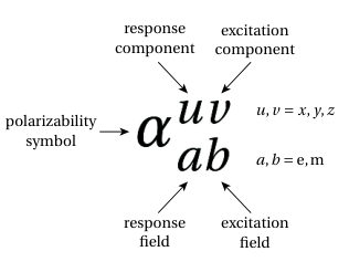
where $\overline{\overline{\alpha}}_{\text{ee}}$, $\overline{\overline{\alpha}}_{\text{em}}$, $\overline{\overline{\alpha}}_{\text{me}}$ and $\overline{\overline{\alpha}}_{\text{mm}}$ are the electric-to-electric, magnetic-to-electric, electric-to-magnetic and magnetic-to-magnetic $3\times{}3$ coupling dyadic tensors, respectively, which are measured in Asm²/V, sm², sm² and Vsm²/A (see Appendix A), and where $\mathbf{E}_{\text{loc}}$ and $\mathbf{H}_{\text{loc}}$ are the local excitation fields. Figure 6 details the notation used in this paper for the components of the polarizability tensors in a Cartesian coordinate system. The local excitation fields are the difference between the global excitation fields and the fields produced by the polarization of the neighboring particles in a dense medium Jackson 1998; Sihvola 1999, and reduce to the excitation fields, $\mathbf{E}$ and $\mathbf{H}$, in a sufficiently dilute medium. The paper assumes that the dilute-medium approximation is valid, until the final design guidelines in Sec. XIII, which does not represents a severe restriction in terms of qualitative description.

According to the rationale in Sec. IV.3, the planar and twisted straight/looped-section metaparticles, which are respectively shown in Figs. 5(a) and 5(b), are both potential candidates for chiral particles, since they both involve magnetoelectric coupling, as we shall verify in Secs. V.3 and V.4. However, according to the definition of Sec. I, such coupling is only a necessary condition for chirality, the absolute (necessary and sufficient condition) criterion being mirror asymmetry (Sec. II). Let us then apply the mirror test, depicted in Fig. 7, to the two metaparticles.

Let us start with the planar Omega particle [Fig. 5(a)], tested in Fig. 7(a). Upon reflection in the $x$, $y$ and $z$ directions, this particle transforms into images that are exactly identical to itself. The $z$ direction image is flipped in space, but can be flipped back, without any structural change, to perfectly superimpose with the original particle, and is hence indeed also identical to it. So, the particle is identical to any of its mirror images. Therefore, it is not chiral or, equivalently, has no handedness. It should therefore not induce any polarization rotation, as shall be verified in Sec. V.3.

How about the twisted Omega or helix particle [Fig. 5(b)], tested Fig. 7(b)? This particle differs from its planar counterpart only by the 90^∘ twist of the loop section with respect to the straight section. However, this volume twist plays a determinant role in the mirror test: the three images are now different from the original particle; they are LH whereas the original one is RH. So, the twisted Omega particle, as the human hand (Fig. 1), is chiral, and we shall see in Sec. V.4 that it possesses the consequently expected polarization rotation property ²² 2 If the $z$-mirrored helix particle were next $y$-mirrored, it would naturally flip handedness again, and hence retrieve the original RH handedness. However, such a double-reflection operation ($z\rightarrow-z$ followed by $y\rightarrow-y$) does not correspond to a reflection in the $xy$ direction but to a rotation of 180^∘ about the $x$ axis. In contrast, yet an additional reflection along $x$ would yield again, as a single reflection, the reverse (LH) handedness. This is because a triple reflection along $x$, $y$ and $z$ ($z\rightarrow-z$, $y\rightarrow-y$, $x\rightarrow-x$) is equivalent to a single reflection in the $xyz$ direction ($\mathbf{r}\rightarrow-\mathbf{r}$)..

Despite the fact that the planar Omega particle is not chiral, we shall still analyze it in the sequel of this section, as its comparison with the twisted Omega or helix particle is instructive for a strong understanding of chirality.

Comparing Fig. 5(b) with Fig. 5(a) shows that the RH helix particle is obtained by twisting the planar particle about the $z$ axis in the clockwise direction, as a key in a lock to open the door, whereas the LH helix particle is obtained by twisting the planar particle about the $z$ axis in the counterclockwise direction, as to close the door. So, the volume twist has imparted handedness, and hence chirality, to the particle.

Such ‘handedness-ization’ would not have been possible without transforming the initially planar structure into a volume one. Indeed, a volume-less, planar structure, such as the planar Omega particle, looks indeed identical from its two sides, and it is only the existence of nonplanarity or volume, as in the helix particle or the hand (Fig. 1) ³³ 3 If the hand had no thickness, it would reduce to its mere projection, and hence have neither a palm nor a back. It would therefore look identical from both sides, and have thus no handedness!, that allows handedness. So, a particle must necessarily include a volume, or thickness, or depth, to be chiral. Moreover, the smallest dimension of this volume must be a significant fraction of the wavelength for a significant chiral effect, since otherwise either the wire section or the loop section would be too small.

However, three-dimensionality is only a necessary condition – and not a sufficient condition! – for chirality. The simplest example demonstrating the latter insufficiency is that of a spherical particle. Also, transforming the planar Omega particle into a volume particle by adding to it untwisted looped sections about the $x$ axis (e.g. in the $xz$ plane) still does not make the particle different from its mirror image and hence chiral.

The $\mathbf{p}_{\text{ee,em}}$ and $\mathbf{p}_{\text{me,mm}}$ dipolar responses of the planar Omega particle, which is now known to be achiral, are depicted in Fig. 8, where the particle lies in the $xz$ plane with its straight section directed along $x$. Let us separately examine the responses to the electric part (top of the figure) and magnetic part (bottom of the figure) of the electromagnetic field excitation to separately determine the electric-response and magnetic-response polarizability pairs $(\overline{\overline{\alpha}}_{\text{ee}},\overline{\overline{\alpha}}_{\text{em}}$) and ($\overline{\overline{\alpha}}_{\text{me}},\overline{\overline{\alpha}}_{\text{mm}}$).

An $x$-directed electric field excitation induces an $x$-directed electric dipole moment $p_{\text{e},{E_{x}}}^{x}$ in the straight section of the particle, which corresponds to the electric-to-electric polarizability $\alpha_{\text{ee}}^{xx}$. The current associated with this dipole moment must then flow in the loop section, due to current continuity, and this occurs in the same (upward in the figure) direction given the subwavelength, $\lambda/2$-dimension of the unfolded particle [Eq. (8)]. This looped current gives rise to the $y$-directed magnetic dipole moment $p_{\text{m},{E_{x}}}^{y}$, which corresponds to the electric-to-magnetic polarizability $\alpha_{\text{me}}^{yx}$. Due to symmetry and due to the subwavelength size of the loop, scattering from the $z$-oriented parts of this (looped) current cancels out, and hence does not produce any $\alpha_{\text{ee}}^{zx}$; in contrast, scattering from its $x$-oriented parts does not cancel out, due to the asymmetry induced by the gap, and therefore slightly contribute to $\alpha_{\text{ee}}^{xx}$.

The response to the magnetic field is found by a symmetric reasoning. A $y$-directed magnetic field excitation induces a $y$-directed magnetic dipole moment $p_{\text{m},{H_{y}}}^{-y}$ in the direction opposing the incident field (Lenz law) in the looped section of the particle, which corresponds to the magnetic-to-magnetic polarizability $\alpha_{\text{mm}}^{yy}$. Due to the same symmetry reason as before, the associated looped current produces a small $\alpha_{\text{em}}^{xy}$ response but no $\alpha_{\text{em}}^{zy}$ response. The looped current must then flow along the straight sections, due to current continuity, and this occurs in the same (downward in the figure) direction given the subwavelength, $\lambda/2$-dimension of the unfolded particle. This straight current gives rise to the $x$-directed electric dipole moment $p_{\text{e},{H_{y}}}^{-x}$, which corresponds to the main part of the magnetic-to-electric polarizability $\alpha_{\text{em}}^{xy}$.

Note that the polarizabilities $\alpha_{\text{me}}^{yx}$ and $\alpha_{\text{em}}^{xy}$ must have the same magnitude since they involve the same geometrical parts. However, they are oppositely directed. Therefore,

One may easily verify that the $E_{x}$–$H_{y}$ polarization considered in Fig. 8 is the only one that yields nonzero polarizabilities, assuming that the conductor forming the particle has a deeply-subwavelength, and hence negligible, diameter ⁴⁴ 4 If the diameter measures a substantial fraction of the wavelength, small responses would also exist in the other directions, leading to extra tensorial components. One could then approximate the different sections by straight and looped ellipsoids, and specifically prolate spheroids with large (needle-type) axis ratio. For instance, if the aspect ratio is $10:1$, the polarizability of a straight needle reads $\alpha=V\epsilon_{0}(\epsilon_{\text{r}}-1)/[1+K(\epsilon_{\text{r}}-1)]=V\epsilon_{0}/K$, assuming that it is perfectly conducting ($\epsilon_{\text{r}}\rightarrow i\infty$), where $V$ is the volume of the needle, $\epsilon_{0}$ the free-space permittivity, and $K$ the depolarization factor in the direction considered. For an $x$-oriented needle, the depolarization factors are found to be $K_{x}=0.02$ and $K_{y}=K_{z}=0.49$ Sihvola 1999. Hence there exists polarizability components perpendicular to the needle axis, but they are $0.49/0.02=24.5$ smaller than that along the axis, and may thus be neglected. So, for sections with a length-to-diameter ratio of more than 10, such effects can be safely ignored.. The global susceptibility tensors of the planar Omega particle in Fig. 8 are then Saadoun and Engheta 1992

The tensor (13) can be modified by transforming the ‘monoatomic’ metaparticle of Fig. 8(a) into a ‘biiatomic’ metaparticle or ‘triatomic’ metaparticle, obtained by adding copies of the initial particle (here in the $xz$ or $zx$ plane) in the other two or three planes. This can be done in a diversity of ways. In each plane, the planar Omega particle can take one out of 4 distinct orientations: the straight section can be directed along the two perpendicular directions of the plane and for each of these orientations the looped section may point to two opposite directions. This may be best seen by using proper labeling. For instance, the particle of Fig. 8(a) may be labelled $(zx,x,+z)$, indicating that it is lying in the $zx$ plane, with straight section in the $x$ direction and looped section pointing towards the $+z$ direction, and the same plane supports also the three other orientations $(zx,x,-z)$, $(zx,z,+x)$ and $(zx,z,-x)$. There are then $4^{1}=4$ possibilities for a monoatomic particle, $4^{2}=16$ possibilities for a biatomic particle, and $4^{3}=64$ possibilities for a triatomic particle.

The triatomic particle corresponding to the cyclic permutations of the particle in Fig. 8(a), i.e., [$(zx,x,+z)$,$(xy,y,+x)$,$(yz,z,+y)$] can be easily found, by the same permutations, to correspond to the metaparticle tensors

where $\overline{\overline{I}}$ and $\overline{\overline{I}}_{\text{P}}$ are the symmetric and permutated unit tensors $\overline{\overline{I}}=\hat{\mathbf{x}}\hat{\mathbf{x}}+\hat{\mathbf{y}}\hat{\mathbf{y}}+\hat{\mathbf{z}}\hat{\mathbf{z}}$ and $\overline{\overline{I}}_{\text{P}}=\hat{\mathbf{x}}\hat{\mathbf{y}}+\hat{\mathbf{y}}\hat{\mathbf{z}}+\hat{\mathbf{z}}\hat{\mathbf{x}}$, respectively. In such a metaparticle, the direct (ee and mm) tensors have reduced to scalar, but the cross (em and me) tensors have not, so that the overall response is still anisotropic.

The most ‘symmetric’ nontrivial medium that can be obtained with the the planar Omega particle is in fact the hexatomic medium with the particles $(zx,x,+z)$ and $(yz,y,+z)$ providing $\hat{\mathbf{z}}\times\overline{\overline{I}}$, $(xy,y,+x)$ and $(zx,z,+x)$ providing $\hat{\mathbf{x}}\times\overline{\overline{I}}$, and $(xy,x,+y)$ and $(yz,z,+y)$ providing $\hat{\mathbf{y}}\times\overline{\overline{I}}$. The corresponding polarizability tensors may be written

where $\overline{\overline{I}}_{\text{A}}$ is the (6-component) antisymmetric tensor $\overline{\overline{I}}_{\text{A}}=\mathbf{r}\times\overline{\overline{I}}$. However, such a metaparticle involves 2 particles per plane, which might be at odds with with the dimensional constraint (8).

Note that allowing more than one planar Omega particle per plane may also wash out the magnetoelectric coupling effects of the resulting multiatomic metaparticle. For instance, if the $zy$ plane were allowed to support the $(zx,x,-z)$ particle in addition to the $(zx,x,+z)$ particle in Fig. 8, then the responses $\alpha_{\text{me}}^{yx}$ and $\alpha_{\text{em}}^{xy}$ would disappear due to cancelation of the scattering from the two particles. The hexaomic metaparticle obtained by adding the two complementary cancelling pairs would naturally lead to a magnetoelectic-less structure.

How about polarization rotation? We have seen above that, for the polarization selected in Fig. 8, the electric response of the metaparticle is fully parallel the electric excitation ($\mathbf{p}_{\text{ee}}\|\mathbf{E}$ and $\mathbf{p}_{\text{em}}\|\mathbf{E}$) and the magnetic response is fully parallel to its magnetic excitation ($\mathbf{p}_{\text{me}}\|\mathbf{H}$ and $\mathbf{p}_{\text{mm}}\|\mathbf{H}$), despite coupling, as may be easily checked in (13),  (14) and (15). This means that the particle does induce any rotation for this polarization. It only induces a phase shift, say $\phi_{x}$, corresponding to its interaction with the wave. But the situation is a little more subtle. Consider now the polarization rotated by 90^∘ (i.e. $\mathbf{E}\|\hat{\mathbf{y}}$ and $\mathbf{H}\|\hat{\mathbf{y}}$). In this case, the particle does essentially not interact with the wave and is hence invisible to it, so that it does not induce any phase shift, or $\phi_{y}=0$. The particle is hence birefringent, which indeed rotates the obliquely polarized incident wave. However, as will be seen in Sec. XI.3, this birefringence is fundamentally different from chiral birefringence, as can readily be realized by the fact that it does not occur for all the incident polarizations.

In summary, we have found that the planar Omega particle in Fig. 8 has the following properties:

1. 1.

   It indeed involves magnetoelectric coupling, as predicted in Sec. IV.3, since $\overline{\overline{\alpha}}_{\text{em}},\overline{\overline{\alpha}}_{\text{me}}\neq 0$, which is the reason it was called pseudo-chiral in Saadoun and Engheta 1992, and $\overline{\overline{\alpha}}_{\text{me}}=-\overline{\overline{\alpha}}_{\text{em}}$;

2. 2.

   Despite such coupling, it is achiral, by definition, since it is identical to its mirror image, as shown in Sec. V.1 (proof of ➄ in Fig. 3);

3. 3.

   It cannot reduce to an isotropic particle upon adding copies in the other two directions of space.

4. 4.

   As expected from its achiral nature (Sec. I) and despite its magnetoelectric coupling, it does not involve systematic polarization rotation, i.e., it is not completely gyrotropic (proof of ➆ in Fig. 3).

The $\mathbf{p}_{\text{ee,em}}$ and $\mathbf{p}_{\text{me,mm}}$ dipolar responses of the twisted Omega or helix particle, which is now known to be chiral, are depicted in Fig. 9, where the straight section is directed along $x$, while the loop section lies in the $yz$ plane. Let us again separately examine the responses to the electric part (top of the figure) and magnetic part (bottom of the figure) of the electromagnetic field excitation to separately determine the electric-response and magnetic-response polarizability pairs $(\overline{\overline{\alpha}}_{\text{ee}},\overline{\overline{\alpha}}_{\text{em}}$) and ($\overline{\overline{\alpha}}_{\text{me}},\overline{\overline{\alpha}}_{\text{mm}}$).

An $x$-directed electric field excitation induces again an $x$-directed electric dipole moment $p_{\text{e},{E_{x}}}^{x}$ on the straight section of the particle, corresponding to $\alpha_{\text{ee}}^{xx}$, and the current associated with this dipole moment again flows in the loop section from current continuity. However, given the $90^{\circ}$ twist of the loop, this current now gives rise to the $x$-directed magnetic dipole moment $p_{\text{m},E_{x}}^{x}$, which corresponds to $\alpha_{\text{me}}^{xx}$. Note in passing the if the angle of the loop twist were not exactly $90^{\circ}$ – e.g. $60^{\circ}$ – then the induced magnetic moment would be tilted, which would introduce parasitic off-axis contributions to the response. Moreover, an $x$-directed magnetic field excitation (different form the $y$-directed one at the bottom of Fig. 8) induces an $x$-directed magnetic dipole moment $p_{\text{m},H_{x}}^{-x}$ in the looped section of the particle, corresponding to $\alpha_{\text{mm}}^{xx}$, plus, from current continuity, the $x$-directed electric dipole moment $p_{\text{e},{H_{y}}}^{-x}$, corresponding to $\alpha_{\text{em}}^{xx}$. Again, the cross polarizations are opposite, i.e.,

In addition, the looped current produces the responses $\alpha_{\text{ee}}^{yx}$ and $\alpha_{\text{em}}^{yx}$ (without $\alpha_{\text{ee}}^{zx}$ and $\alpha_{\text{em}}^{zx}$) due to the gap asymmetry; however, these responses are negligibly small as the $yz$ plane projection of the gap is very small and may even reach zero, and we therefore henceforth consider them negligible. These observations indicate that a mirror asymmetry, corresponding to a volume twist, necessarily induces magnetoelectric coupling (proof of ➂ in Fig. 3).

So, the four main susceptibilities identified above correspond to the dyadic component $xx$, and it is easy to verify that all the other susceptibility components are negligible. The helix metaparticle in Fig. 9 has thus the polarizability tensors

and the ‘triatomic’ metaparticle formed by adding copies of that particle in the $y$ and $z$ directions, as shown in Fig. 10, has the polarizability tensors

which have this time reduced to scalars. Remarkably, and in contrast with the 64 possibilities of the straight Omega particle, this arrangement the helix particle is unique ⁵⁵ 5 This, of course, assumes only one type of handedness, either RH or LH. If we allow both LH and RH particles, we have $2^{3}=8$ possible combinations (2 handednesses in each of the 3 directions of space). However, 6 of these combinations lead to different signs in different directions, which breaks biisotropy. The arrangement of Fig. 10 – and its LH counterpart whose $\chi$ has the opposite sign – are the only ones yielding purely scalar polarizabilities, or biisotropy (see Secs. VII.2 and VII.3).! In this sense, the helix particle is much more symmetric and fundamental than the planar Omega particle.

Given the particle chirality, we expect to have here polarization rotation. Indeed, we have, along with $\mathbf{p}_{\text{ee}}\|\mathbf{E}$ and $\mathbf{p}_{\text{mm}}\|\mathbf{H}$, that $\mathbf{p}_{\text{me}}\perp\mathbf{H}$ and $\mathbf{p}_{\text{em}}\perp\mathbf{E}$, indicating that part of the magnetic field and electric field have been rotated by 90^∘, which is a clear indication the expected gyrotropy. Specifically, the initially $+y$-directed field $\mathbf{H}$ (top of the figure) has rotated towards the $+x$ direction into $p_{\text{m},E_{x}}^{x}$, while the initially $-y$-directed field $\mathbf{E}$ (bottom of the figure) has rotated towards the $-x$ direction into $p_{\text{e},{H_{x}}}^{-x}$. The electromagnetic field has therefore rotated about the $z$ axis in the direction corresponding to the left-hand with the thumb pointing in the propagation direction ($+z$). In other words, the field phasors associated with the cross coupling terms have rotated by the angle of $-\pi/2$ ($y$ to $x$ direction) or, equivalently, have been multiplied by the factor $e^{-i\pi/2}=-i$, and therefore the cross coupling polarizabilities are in quadrature with their direct coupling counterparts. A LH particle naturally leads to rotation in the opposite direction.

In contrast to the planar Omega particle (Fig. 8), the twisted Omega or helix particle involves two different polarization states in its nonzero polarizabilities. Specifically, in Fig. 9, the polarization $(E_{x},H_{y})$ involves $\alpha_{\text{ee}}^{xx}$ and $\alpha_{\text{me}}^{xx}$, while the polarization $(-E_{y},H_{x})$ involves $\alpha_{\text{mm}}^{xx}$ and $\alpha_{\text{em}}^{xx}$. In the case of a circularly polarized exciting wave, these two states are separated by the time interval $T/4$ ($T=\omega/(2\pi)$: time period) of the harmonic wave, which correspond to a factor $e^{-i\pi/2}=-i$ in phasor notation. These observations indicate mirror asymmetry necessarily induces polarization rotation (proof of ➁ in Fig. 3).

In summary, we have found that the twisted Omega or helix particle in Fig. 8 has the following properties:

1. 1.

   It indeed involves magnetoelectric coupling, as predicted in Sec. IV.3, since $\overline{\overline{\alpha}}_{\text{em}},\overline{\overline{\alpha}}_{\text{me}}\neq 0$, and $\overline{\overline{\alpha}}_{\text{me}}=-\overline{\overline{\alpha}}_{\text{em}}$;

2. 2.

   It is chiral, by definition, since it is different to its mirror image, as shown in Sec. V.1, as allowed by its volume configuration (Sec. V.2);

3. 3.

   It reduces to an isotropic particle upon adding copies in the other two directions of space, since the response is then purely diagonal.

4. 4.

   As expected from its chiral nature (Sec. I), it induces polarization rotation, i.e., it is gyrotropic.

5. 5.

   The polarizability pairs ($\alpha_{\text{ee}}^{xx},\alpha_{\text{me}}^{xx}$) and ($\alpha_{\text{mm}}^{xx},\alpha_{\text{em}}^{xx}$) are in a quadrature relationship.

Analytical formulas for the values of the polarizabilities of the helix particle in terms of its geometrical parameters are given in Tretyakov et al. 1996. Alternative chiral particles may be easily inferred from the observations made in this section. First, a chiral particle must necessarily have a volume, according to Sec. V.2, which disqualifies all purely planar particles. Even twisted planar particles, such as all kinds of gammadion crosses, are achiral. Such structures have a sort of handedness, but this is a weak form of handedness, since it changes with the side from which they are observed, so that they are identical to their mirror image. However, chiral particles may take alternative shapes, such their multiturn-helix, or spring, version in Fig. 4, their square-loop version of the helix in Fig. 5, or structures looking like that the amino acids represented in Fig. 2.

The behavior of an electromagnetic medium can generally be expressed by the relations Kong 2008; Jackson 1998; Ishimaru 2017

where $\epsilon_{0}\mathbf{E}$ and $\mu_{0}\mathbf{H}$ respectively represent the electric and magnetic responses of free space, which corresponds to the spacings between the molecules or metaparticles, while the $\mathbf{P}_{\text{e}}$ and $\mathbf{P}_{\text{e}}$ represents the response of the particle forming the medium and given by (21). Equations (22) correspond to the most usual electromagnetics convention of $[\mathbf{D};\mathbf{B}]$ being expressed in terms of $[\mathbf{E};\mathbf{H}]$, where $\mathbf{E}$ and $\mathbf{H}$ are considered as the excitations while $\mathbf{B}$ and $\mathbf{D}$ are considered as the medium responses Jackson 1998; Ishimaru 2017 ⁶⁶ 6 The book Kong 2008 also includes the alternative formulations $[\mathbf{D};\mathbf{H}]$ versus $[\mathbf{E};\mathbf{B}]$, based on the motivation that $\mathbf{E}$ and $\mathbf{B}$ are the fields that are directly measurable experimentally via the Lorentz force ($\mathbf{F}=q\left(\mathbf{E}+\mathbf{v}\times\mathbf{B}\right)$; $q$: charge, $\mathbf{v}$: charge velocity), and $[\mathbf{E};\mathbf{H}]$ versus $[\mathbf{D};\mathbf{B}]$, based on the motivation that $\mathbf{D}$ and $\mathbf{B}$ form with the spectral spatial wavevector $\mathbf{k}$ an electromagnetic basis that does not dependent on the nature of the medium..

We now relate the field responses to the medium susceptibilities by inserting (21) into (22), which yields

Defining

transforms (23) into the conventional bianisotropic ⁷⁷ 7 In the term ‘bianisotropic’, coined by Kong in Cheng and Kong 1968, ‘bi’ refers to the fact that each (electric and magnetic) response depends on both the electric excitation and the magnetic excitation, while ‘anisotropic’ refers to the fact the responses are not parallel to their excitations or, equivalently, are characterized by tensorial parameters. From (20), it is clear that this term applies to the polarizabilities as well as to the susceptibilities. relations Kong 1972; Lindell et al. 1994; Kong 2008

where $\overline{\overline{\epsilon}}$, $\overline{\overline{\mu}}$, $\overline{\overline{\xi}}$ and $\overline{\overline{\zeta}}$ are the permittivity, permeability, magnetic-to-electric coupling and electric-to-magnetic coupling dyadic tensors, respectively, which are measured in As/Vm, Vs/Am and s/m (see Appendix A). The four medium tensors are generally of dimension $3\times 3$, and involve thus 36 complex parameters overall.

The coupled equations (25) – where $\mathbf{D}$ and $\mathbf{B}$ are interdependent through the coupling tensors $\overline{\overline{\xi}}$ and $\overline{\overline{\zeta}}$ – represent the most general explicit constitutive relations for an LTI medium. Linear time-invariance [Assumption 1) in Sec. III] is indeed a necessary condition for such relations to hold, since nonlinearity would involve powers of $\mathbf{E}$ and $\mathbf{H}$ Boyd and Prato 2008, while time variance would require replacing the scalar products by convolution products Kalluri 2010.

As we have seen in Sec. V.3, the straight Omega particle [Fig. 5(a) or Fig. 8(a)], whether unique or combined with copies of itself in different directions of space, is always characterized by non-reducible bianisotropic relations [Eqs. (13), (14) and (15)]. Therefore, they correspond to the most general relations (25), whose tensorial parameters are obtained from (13), (14) or (15) via (20).

In the particular case where the tensors $\overline{\overline{\epsilon}}$, $\overline{\overline{\mu}}$, $\overline{\overline{\xi}}$ and $\overline{\overline{\zeta}}$ in (25) reduce to $\epsilon\overline{\overline{I}}$, $\mu\overline{\overline{I}}$, $\xi\overline{\overline{I}}$ and $\zeta\overline{\overline{I}}$, and hence ultimately to scalars, the medium is called biisotropic. This is for instance the case of the medium formed by the triatomic helix particle shown in Fig. 10 and characterized by the polarizability tensor (18). Equations (25) reduce then to

and a biisotropic medium is thus characterized only by the 4 complex parameters $\epsilon$, $\xi$, $\zeta$ and $\mu$.

We have established in Sec. V.4 that the cross coupling parameters of a chiral structure were opposite to each other [Eq. (16)] and in quadrature with the direct coupling parameters (Fig. 9). In terms of the constitutive parameters in (26), this translates into

where the last equality expresses the fact the the electric and magnetic responses of a plane wave in a simple biisotropic medium – such as free space – are in phase, as seen by inserting (4) into (5). In order to make sure to select the correct signs in (27), let us examine the behavior of the RH helix particle described in Fig. 9 in some more details.

For this purpose, Fig. 11 isolates and compares the electric and magnetic responses to the electric and magnetic fields. The figure first recalls the result established in conjunction with Fig. 9 that the RH helix particle rotates the field polarization in the transverse plane in the direction corresponding to the left hand with the thumb pointing in the propagation direction, or in the $y$ to $x$ direction, corresponding to phasor multiplication by the factor $(-i)$, or yet to a delay $T/4=(2\pi/\omega)/4=\pi/(2\omega)$. Comparing the responses $\mathbf{D}_{\mathbf{E}}$ and $\mathbf{D}_{\mathbf{H}}$ shows then that the latter is $\pi/2$ beyond (or $T/4$ later) in the mentioned direction than the former; it must therefore be rotated backward, in the positive ($x$ to $y$) direction, for matching (or synchronization), or multiplied by the factor $+i$. Similarly comparing the responses $\mathbf{B}_{\mathbf{H}}$ and $\mathbf{B}_{\mathbf{E}}$ shows that the latter is $\pi/2$ behind (or $T/4$ earlier) in the mentioned direction than the former; it must therefore be rotated forward, in the negative ($y$ to $z$) direction, for matching (or synchronization), or multiplied by the factor $-i$. Opposite signs would naturally be obtained in the case of a LH helix particle.

We have thus, with respect to the references of $\epsilon$ and $\mu$, that $\xi=+i\chi$ and $\zeta=-i\chi$. This reformulates the chiral constitutive relations (26) as

where $\chi$ is called the chiral parameter, which be shown in Sec. VII.4 to be purely real in the lossless case and complex in the presence of loss Lindell et al. 1994; Kong 2008. A chiral medium, characterized by the relations (28), is also called a Pasteur medium. Inserting (28) into (5) provides then the following explicit form of Maxwell equations for a chiral or Pasteur medium:

Note the Greek symbol $\chi$ is now associated with both the susceptibility, from (21), and with the chirality factor, from (28). However, the former will always appear with the double subscript ee, em, me or mm, whereas the latter is always on its own. So, this coincidence should not pose any notational ambiguity.

The reciprocity of a chiral medium, which is imposed by the assumed absence of an external force or of nonlinearity combined with spatial asymmetry Caloz and Itoh 2005, is expressed in the constitutive relations (28) by the fact that $\overline{\overline{\xi}}=i\chi\overline{\overline{I}}=-\overline{\overline{\zeta}}$ satisfies the reciprocity condition

where the subscript $T$ denotes the transpose operation, and which results from the Lorentz nonreciprocity relations Kong 2008; Caloz et al. 2018.

As we have seen in Sec. V.4, the metamaterial constituted by the triatomic helix metaparticle shown in Fig. 10 is isotropic [Eq. (18)]. Therefore, it indeed corresponds to the biisotropic chiral relations (28). Such a medium is represented in Fig. 12. However, the monoatomic helix particle in Fig. 5, described by the anisotropic polarizability tensors (17), is also chiral and gyrotropic, as shown in Fig. 9. This indicates that the biisotropic formulation (28) is excessively restrictive. However, it is what is generally called chirality (actually meaning biisotropic chirality) in the electromagnetic community, and we shall not dispute this term here.

The chiral relations (28) do not not represent the only form of biisotropy. The magnetoelectric responses can also be in phase with their responses. In this case, we can write $\xi=\tau$ and $\zeta=\tau$, which particularizes (26) to

where $\tau$ will also be shown in Sec. VII.4 to be purely real in the lossless case and complex in the presence of loss. These equations (31) are the constitutive relations of a Tellegen medium. Such medium is nonreciprocal since $\overline{\overline{\xi}}=\tau\overline{\overline{I}}=\overline{\overline{\zeta}}=\overline{\overline{\zeta}}^{T}$ violates the reciprocity condition (30). Therefore, it must involve an external force, specifically permanent or induced electric and magnetic dipole moments parallel or antiparallel to each other Lindell et al. 1994.

Thus, the coupling parameters $\xi$ and $\zeta$ of a biisotropic medium [Eq. (26)] may generally be written as Lindell et al. 1994; Kong 2008

Inserting (32) into (26) provides the alternative general biisotropic constitutive relations

which correspond to a chiral of Pasteur medium if $\tau=0$ and $\chi\neq 0$ and to a Tellegen medium if $\tau\neq 0$ and $\chi=0$.

It is useful to relate the three parameters $\epsilon$, $\mu$ and $\chi$ in (28) to the corresponding susceptibilities, which are then obtainable from the metaparticle polarizabilities via (20). These relations may be found by reducing the tensors to scalars in (24) and using (32) with $\tau=0$, i.e., $\xi=i\chi$ and $\zeta=-i\chi$, which yields

implying that $\chi_{\text{me}}=-\chi_{\text{em}}$, consistently with the previously found results for the twisted Omega or helix particle (Sec. V.4).

According to the Poynting theorem, a medium is lossless if the divergence of the divergence of its Poynting vector in it is always purely imaginary Jackson 1998; Ishimaru 2017, i.e.,

where the ‘*’ superscripts denotes the complex conjugate operation. The divergence in (35) can be expanded as follows:

where we have applied the identity $\nabla\cdot(\mathbf{a}\times\mathbf{b})=\mathbf{b}\cdot(\nabla\times\mathbf{a})-\mathbf{a}\cdot(\nabla\times\mathbf{b})$ in the second equality, and replaced $\nabla\times\mathbf{E}$ and $\nabla\times\mathbf{H}$ by their Maxwell expressions (29). Nullifying the real part of the last expression in (36) according to (35) finally yields the lossless conditions

The demonstration of these relations may go as follows. First consider a point of space and phase of the harmonic cycle where $\mathbf{H}=0$. At such a point, Eq. (36) implies (37a), and that relation must always be true since the medium is assumed to be time invariant. Then consider another point and phase where $\mathbf{E}=0$, which now implies (37b). This leaves out only the third term in the last expression of (36). The factor $\chi-\chi^{*}$ in this term is purely imaginary, but it still must vanish for if it would not, then $\mathbf{E}\cdot\mathbf{H}^{*}$, which is generally complex and thus includes an imaginary part, would otherwise assign a real part to the overall term in violation to the the zero real requirement. Note in passing that it is easy to verify that in a Tellegen medium $\tau$ is also purely real in the lossless case and complex in the lossy case.

In the presence of loss, the parameters $\epsilon$, $\mu$ and $\chi$ may be complex, i.e.,

where the primed and unprimed quantities are real numbers denoting the real and imaginary parts. Therefore, the RH and LH eigenwavenumbers, which will be derived in Sec. IX.1 as $\beta^{+}_{\pm}=\omega(\sqrt{\epsilon\mu}\pm\chi)$ [Eq. (45a)], generally do not have only different real parts but also different imaginary parts, and then different absorptions. This difference in absorption for the RH and LH waves results in transforming the lossless circularly polarized states into elliptical polarized states, as will become clear in Sec. IX.2. This phenomenon is referred to as circular dichroism Gasman 2013.

Finally, note that the imaginary parts of ($\epsilon,\chi_{\text{ee}}$) and ($\mu,\chi_{\text{mm}}$) are purely positive in a lossy (or dissipative) medium with the assumed $e^{-i\omega t}$ harmonic time dependence (Appendix B). In contrast, the passive lossy condition on ($\chi,\chi_{\text{em,me}}$) is less restrictive Lindell 1992; for $\chi$, this condition is found from $\text{Im}\{\beta^{+}_{\pm}\}>0$ as $\text{Im}\{\chi\}<\text{Im}\{\sqrt{\epsilon\mu}\}$.

References

- Arago (1812) D. F. J. Arago, “Mémoire sur une modification remarquable qu’éprouvent les rayons lumineux dans leur passage à travers certains corps diaphanes et sur quelques autres nouveaux phénomènes d’optique,” Ann. Chem. Phys 2, 372–389 (1812), mémoire présenté le 11 août 1811.
- Biot (1814) J.-B. Biot, Mémoires sur un nouveau genre d’oscillation que les molécules de la lumière éprouvent en traversant certains cristaux (Chez Firmin Didot, 1814).
- Fresnel (1868) A. Fresnel, Oeuvres Complètes d’Augustin Fresnel (Imprimerie impériale, 1868) vol. 1:731-51; vol. 2:479-596.
- Pasteur (1850) L. Pasteur, Recherches sur les propriétés spécifiques des deux acides qui composent l’acide racémique (Impr. Bachelier, 1850).
- Bose (1898) J. C. Bose, “On the rotation of plane of polarization of electric waves by twisted structure,” Proc. Royal Soc. 63, 146–152 (1898).
- Lindman (1914) K. F. Lindman, “Om en genom ett isotropt system av spiralformiga resonatorer alstrad rotationspolarisation av de elektromagnetiska vågorna,” Öfversigt af Finska Vetenskaps-Societetens förhandlingar, A 57, 1–32 (1914).
- Condon (1937) E. U. Condon, “Theories of optical rotatory power,” Rev. Modern Phys. 9, 432–457 (1937).
- Tellegen (1948) B. D. H. Tellegen, “The gyrator, a new electric network element,” Philips Res. Rep. 3, 81–101 (1948).
- Post (1962) E. J. Post, Formal Structure of the Electromagnetics (North-Holland, 1962).
- Kong (1972) J. A. Kong, “Theorems of bianisotropic media,” Proc. IEEE 60, 1036–1046 (1972).
- Fedorov (1976) F. I. Fedorov, Teoria Girotropii (Nauka i Technika, 1976).
- Lakhtakia et al. (1962) A. Lakhtakia, V. K. Varadan, and V. V. Varadan, Time-harmonic Electromagnetic Fields in Chiral Media, Vol. 335 (Springer, 1962).
- Lindell et al. (1994) I. V. Lindell, A. H. Sihvola, S. A. Tretyakov, and A. J. Viitanen, Electromagnetic Waves in Chiral and Bi-Isotropic Media (Artech, 1994).
- Kong (2008) J. A. Kong, Electromagnetic Wave Theory (EMW Publishing, 2008).
- Capolino (2009) F. Capolino, ed., Metamaterials Handbook (CRC Press, 2009) 2 volumes.
- Achouri and Caloz (2018) K. Achouri and C. Caloz, “Design, concepts, and applications of electromagnetic metasurfaces,” Nanophotonics 7, 1095–1116 (2018).
- Born and Wolf (1999) M. Born and E. Wolf, Principles of Optics: Electromagnetic Theory of Propagation, Interferance and Diffraction of Light, seventh ed. (Cambridge University Press, 1999).
- Caloz et al. (2018) C. Caloz, A. Alù, S. Tretyakov, D. Sounas, K. Achouri, and Z.-L. Deck-Léger, “Electromagnetic nonreciprocity,” Phys. Rev. Appl. 10, 047001:1–26 (2018).
- Jackson (1998) J. D. Jackson, Classical Electrodynamics, 3rd ed. (Wiley, 1998).
- Landau et al. (1984) L. D. Landau, L. P. Pitaevskii, and E. M. Lifshitz, Electrodynamics of Continuous Media, 2nd ed., Course of theoretical physics, Vol. 8 (Butterworth-Heinemann, 1984) Chap. XII.
- Harrington (1961) R. F. Harrington, Time-Harmonic Electromagnetic Fields (McGraw-Hill, 1961).
- Pozar (2011) D. M. Pozar, Microwave Engineering, 4th ed. (Wiley, 2011).
- Clemmow (1996) P. C. Clemmow, The Plane Wave Spectrum Representation of Electromagnetic Fields, The IEEE/OUP Series on Electromagnetic Wave Theory (IEEE Press, 1996) classical reissue.
- Sihvola (1999) A. H. Sihvola, Electromagnetic Mixing Formulas and Applications (IET, 1999).
- (25) In general, a multipole expansion is required for modeling the scattering from an object Jackson 1998. However, the multipoles of order larger than the dipoles have a negligible effect when the object is deeply subwavelength, as is the case for a metaparticle, according to (8).
- Caloz and Itoh (2005) C. Caloz and T. Itoh, Electromagnetic Metamaterials: Transmission Line Theory and Microwave Applications (Wiley and IEEE Press, 2005).
- Shelby et al. (2001) R. A. Shelby, D. R. Smith, and S. Schultz, “Experimental verification of a negative index of refraction,” Science 292, 77–79 (2001).
- Ishimaru (2017) A. Ishimaru, Electromagnetic Wave Propagation, Radiation, and Scattering: From Fundamentals to Applications, 2nd ed. (Wiley - IEEE Press, 2017).
- (29) If the -mirrored helix particle were next -mirrored, it would naturally flip handedness again, and hence retrieve the original RH handedness. However, such a double-reflection operation ( followed by ) does not correspond to a reflection in the direction but to a rotation of 180∘ about the axis. In contrast, yet an additional reflection along would yield again, as a single reflection, the reverse (LH) handedness. This is because a triple reflection along , and (, , ) is equivalent to a single reflection in the direction ().
- (30) If the hand had no thickness, it would reduce to its mere projection, and hence have neither a palm nor a back. It would therefore look identical from both sides, and have thus no handedness!
- (31) If the diameter measures a substantial fraction of the wavelength, small responses would also exist in the other directions, leading to extra tensorial components. One could then approximate the different sections by straight and looped ellipsoids, and specifically prolate spheroids with large (needle-type) axis ratio. For instance, if the aspect ratio is , the polarizability of a straight needle reads , assuming that it is perfectly conducting (), where is the volume of the needle, the free-space permittivity, and the depolarization factor in the direction considered. For an -oriented needle, the depolarization factors are found to be and Sihvola 1999. Hence there exists polarizability components perpendicular to the needle axis, but they are smaller than that along the axis, and may thus be neglected. So, for sections with a length-to-diameter ratio of more than 10, such effects can be safely ignored.
- Saadoun and Engheta (1992) S. M. I. Saadoun and N. Engheta, “A reciprocal phase shifter using novel pseudochiral or medium,” Microw. Opt. Technol. Lett. 5, 184–188 (1992).
- (33) This, of course, assumes only one type of handedness, either RH or LH. If we allow both LH and RH particles, we have possible combinations (2 handednesses in each of the 3 directions of space). However, 6 of these combinations lead to different signs in different directions, which breaks biisotropy. The arrangement of Fig. 10 – and its LH counterpart whose has the opposite sign – are the only ones yielding purely scalar polarizabilities, or biisotropy (see Secs. VII.2 and VII.3).
- Tretyakov et al. (1996) S. A. Tretyakov, F. Mariotte, C. R. Simovski, T G. Kharina, and J.-P. Heliot, “Analytical antenna model for chiral scatterers: comparison with numerical and experimental data,” IEEE Tran. Antennas Propag. 44, 1006–1014 (1996).
- Collin (1990) R. E. Collin, Field Theory of Guided Waves, 2nd ed. (Wiley-IEEE Press, 1990) chap. 12: “Artificial Dielectrics”.
- (36) The book Kong 2008 also includes the alternative formulations versus , based on the motivation that and are the fields that are directly measurable experimentally via the Lorentz force (; : charge, : charge velocity), and versus , based on the motivation that and form with the spectral spatial wavevector an electromagnetic basis that does not dependent on the nature of the medium.
- (37) In the term ‘bianisotropic’, coined by Kong in Cheng and Kong 1968, ‘bi’ refers to the fact that each (electric and magnetic) response depends on both the electric excitation and the magnetic excitation, while ‘anisotropic’ refers to the fact the responses are not parallel to their excitations or, equivalently, are characterized by tensorial parameters. From (20), it is clear that this term applies to the polarizabilities as well as to the susceptibilities.
- Boyd and Prato (2008) R. W. Boyd and D. Prato, Nonlinear Optics, 3rd ed. (Academic Press, 2008).
- Kalluri (2010) D. K. Kalluri, Electromagnetics of time varying complex media: frequency and polarization transformer (CRC Press, 2010).
- Gasman (2013) G. D. Gasman, Circular Dichroism and the Conformational Analysis of Biomolecules, seventh ed. (Springer Science & Business Media, 2013).
- Lindell (1992) I. V. Lindell, Methods for Electromagnetic Field Analysis (Wiley-IEEE Press, 1992).
- (42) We have by definition [Eq. (39)] (mirror symmetry), (return to original spatial frame), (mirror symmetry), etc., which is rather trivial. The situation is more subtle when rotations in different directions are involved, as in Sec. V.1.
- (43) This corresponds to the polarization handedness convention generally used in the electrical engineering community (e.g. Kong 2008; Pozar 2011; Balanis 2012; Ulaby and Ravaioli 2014), for which all the results following the time-harmonic convention (used in this paper) apply upon substituting for transformation to the time-harmonic convention (e.g., Eq. (46): the resulting opposite signs in both the complex vector and the complex phase eventually cancel out to yield the same real result.). The physics and optics community generally follows a convention leading to the opposite handedness, referring to clock direction rather than handedness, and considering that when the field rotation is counterclockwise (resp. clockwise) with the observer facing the oncoming wave, the wave is left-handed (resp. right-handed) (e.g. Jackson 1998; Saleh and Teich 2007). This is all quite confusing, but important to note!
- Ulaby and Ravaioli (2014) F. T. Ulaby and U. Ravaioli, Fundamentals of Applied Electromagnetics, seventh ed. (Pearson, 2014).
- (45) Here, we chose to reverse the sign of while leaving the sign of unchanged. Doing the opposite would transform (47a) to the equivalent result in the reversed coordinate system, where the reversal of the sign of compared to (45a) is a manifestation of this space-reversal odd symmetry of chirality [Eq. (45a)].
- Dionne et al. (2005) G. F. Dionne, G. A. Allen, P. R. Haddad, C. A. Ross, and B. Lax, “Circular polarization and nonreciprocal propagation in magnetic media,” Lincoln Lab. J. 15, 323–340 (2005).
- Lax and Button (1962) B. Lax and K. J. Button, Microwave Ferrites and Ferrimagnetics (McGraw-Hill, 1962).
- Faraday (1933) M. Faraday, Faraday’s Diary, edited by T. Martin (George Bell and Sons, 1933) vol. IV, Nov. 12, 1839 - June 26, 1847.
- Stix (1992) T. H. Stix, Waves in Plasmas (American Institute of Physics, 1992).
- Kodera and Caloz (2018) T. Kodera and C. Caloz, “Unidirectional Loop Metamaterial (ULMs) as as magnetless ferrimagnetic materials: principles and applications,” IEEE Antennas Wirel. Propag. Lett. 17, 1943–1947 (2018).
- Hehl and Obukhov (2003) F. W. Hehl and Y. N. Obukhov, Foundations of Classical Electrodynamics (Birkhäuser Boston, 2003).
- (52) The non-explicit nature of (28) can be easily realized by trying to write a response-field component as a function of the excitation-field components. For instance, Eq. (28a) implies . But, this relation is incomplete per se, because it is coupled to (28b), where may be written as . Substituting this relation into the previous one yields . Now coupling is accounted for, but the electric-response component does not depend only on the electric excitation () but also on the magnetic-excitation component , and it is not possible to go any further.
- (53) This is well-known to be the case in regular plasmas, where the plasma frequency of the conduction electrons is given by , where , and are the density, charge and effective mass of these electron Jackson 1998, but this is also true in metamaterials, as shown in Pendry et al. 1999 for split-ring resonators upon safely defining the effective permeability as the ratio of the and fields.
- Tretyakov et al. (2003) S. A. Tretyakov, I. Nefedov, A. Sihvola, S. Maslovski, and C. Simovski, “Waves and energy in chiral nihility,” J. Electromag. Waves Appl. 17, 695–706 (2003).
- Cheng and Kong (1968) D. K. Cheng and J.-A. Kong, “Covariant descriptions of bianisotropic media,” Proc. IEEE 56, 248–251 (1968).
- Balanis (2012) C. A. Balanis, Advanced Engineering Electromagnetics, 2nd ed. (Wiley, 2012).
- Saleh and Teich (2007) B. E. A. Saleh and M. C. Teich, Fundamentals of Photonics, 2nd ed. (Wiley-Interscience, 2007).
- Pendry et al. (1999) J. B. Pendry, A. J. Holden, D. J. Robbins, and W. J. Stewart, “Magnetism from conductors and enhanced nonlinear phenomena,” IEEE Trans. Microw. Theory Tech. 47, 2075–2084 (1999).
- (59) Private communication with D. L. Sounas.
- (60) In Maxwell equations, the differential operator refers to space, i.e., , and applies to electromagnetic waves, which, assuming linearity, decompose in plane waves, Clemmow 1996. We have then that or, more generally, , whose units is clearly rad/m.
- (61) This may be demonstrated ad absurdum as follows Sou. If we had (reflection rotation), then we would also have, from isotropy, and . The latter result following from the fact that the wave would rotate in the same direction for the two experiments (given the same particle chirality), so that and . But reciprocity (or time-reversal symmetry) requires . Therefore, one must have , i.e., no reflection rotation.
Appendices
Appendix A Units of the Polarizabilities and of the Constitutive Parameters
The units of the polarizabilities may be found by the definitions (11) as