Latent Simplex Position Model:
High Dimensional Multi-view Clustering
with Uncertainty Quantification
Abstract: High dimensional data often contain multiple facets, and several clustering patterns can co-exist under different variable subspaces, also known as the views. While multi-view clustering algorithms were proposed, the uncertainty quantification remains difficult — a particular challenge is in the high complexity of estimating the cluster assignment probability under each view, and sharing information among views. In this article, we propose an approximate Bayes approach — treating the similarity matrices generated over the views as rough first-stage estimates for the co-assignment probabilities; in its Kullback-Leibler neighborhood, we obtain a refined low-rank matrix, formed by the pairwise product of simplex coordinates. Interestingly, each simplex coordinate directly encodes the cluster assignment uncertainty. For multi-view clustering, we let each view draw a parameterization from a few candidates, leading to dimension reduction. With high model flexibility, the estimation can be efficiently carried out as a continuous optimization problem, hence enjoys gradient-based computation. The theory establishes the connection of this model to a random partition distribution under multiple views. Compared to single-view clustering approaches, substantially more interpretable results are obtained when clustering brains from a human traumatic brain injury study, using high-dimensional gene expression data.
KEYWORDS: Co-regularized Clustering, Consensus, PAC-Bayes, Random Cluster Graph, Variable Selection
1 Introduction
High dimensional data are becoming increasingly common in areas such as genomics, computer vision, neuroscience, etc. They are characterized by the ambient dimension substantially larger than the sample size . When clustering such data, canonical solutions tend to focus on finding one particular clustering pattern. For example, one idea is to use variable selection method to identify a small subset of variables with large discriminability, then using them as input for clustering algorithms (Law et al. 2003; Tadesse et al. 2005; Hoff 2006; Witten and Tibshirani 2010); another idea is to reduce the dimension onto latent linear subspaces, often via a Gaussian mixture model with low-rank covariance structure (Ghahramani and Hinton 1996); recent work extends this to the variational autoencoder for nonlinear dimension reduction (Dilokthanakul et al. 2016). These methods have been successful when there is only one clear clustering result in the data. However, as high dimension data often contain multiple facets of the observations, it is more natural to consider more than one clustering patterns — that is, different subspaces of variables can correspond to distinct clustering results. As a result, focusing on one clustering pattern — or, ‘single-view’ is often inadequate.
There has been active literature motivated for ‘multi-view clustering’. Since there are two distinct definitions of this concept, to be clear, we will focus on the one finding multiple clustering patterns, as opposed to the other aiming for one consensus based on multiple data sources. Within our scope, early work includes combining random projection and spectral clustering to obtain clusters on a randomly projected space, repeating this several times to produce multiple clustering patterns (Fern and Brodley 2003); using regularization framework by running clustering algorithm in each view, while minimizing the cross-view divergence (Kumar et al. 2011; Joshi et al. 2016).
As clusters tend to overlap, there is often substantial uncertainty in clustering. A major interest is on the randomness of cluster assignment, characterized by a categorical distribution. In the canonical single-view setting, one typically relies on the Bayesian framework by assigning a model-based likelihood (Fraley and Raftery 2002). This requires putting a parametric assumption on each within-cluster distribution, then estimating the posterior of cluster assignment via the Markov-chain Monte Carlo (MCMC) algorithm. Among the Bayesian multi-view clustering literature (Niu et al. 2010; Li and Shafto 2011; Kirk et al. 2012; Lock and Dunson 2013; Niu et al. 2013; Mo et al. 2017), Guan et al. 2010 and Niu et al. 2012 use the Indian Buffet Process to combine relevant variables into several groups, and in each group, they use a Gaussian mixture model to carry out clustering. These Bayesian models give a generative perspective for the multi-view data; however, there are two major challenges in practice: 1) assigning a within-cluster distribution is prone to misspecifying the model, which leads to breakdown of the parameter estimation (Hennig et al. 2004) and uncontrolled growth in the number of clusters (Miller and Dunson 2018); 2) the MCMC computation suffers from a critically slow convergence/mixing as the dimension grows, limiting its high dimension application. For the former, it was recently shown that modeling the pairwise divergence has much better robustness compared to the original data (Duan and Dunson 2018); for the latter, in general, it has become increasingly popular to replace sampling with an optimization-based approximation for the posterior distribution (El Moselhy and Marzouk 2012).
In this article, we are motivated for an approximate Bayes approach that allows for a direct estimation of the cluster assignment and co-assignment probabilities, within the scope of having several distinct clustering patterns. This is inspired by the resemblance between a similarity matrix and a cluster graph, hence the former can be considered as a noisy version of the latter. In the community detection literature, one often learns a low-rank representation for each data point as the latent position in Euclidean/Stiefel space (Hoff et al. 2002), then cluster the coordinates into communities (Handcock et al. 2007). Instead of going through two modeling stages, we put the latent coordinates directly on the probability simplex, describing the probabilities for cluster assignment and allowing gradient-descent optimization; in the meantime, each co-assignment matrix is a random draw out of only a few candidate parameterizations, leading to dimension reduction and information sharing among views.
2 Method
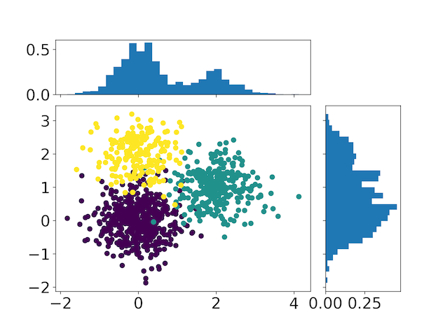
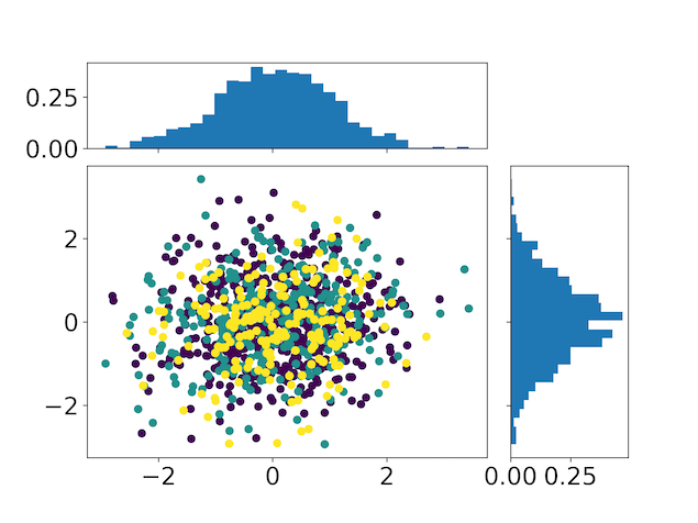
Let be the data over . Each is a multi-dimensional vector, and we can separate its elements into groups of sub-vectors . We will now call the subspace for as a ‘view’ of the data. To help explain the idea, we use a running example of simulated data over views (each in ). Figure 1 shows the scatter plots.


Assuming the views are given, our goal is to obtain clustering for each view, in particular, a discrete label corresponding to the cluster assignment for each . Equivalently, we can focus on the co-assignment for each pair of data
where is the indicator function taking if is true, otherwise taking .
2.1 Latent Simplex Position Model
Treating as an adjacency matrix, we can form a cluster graph: , with and . In this graph, each cluster forms a complete sub-graph (all pairs of nodes within are connected), and the sub-graphs are disconnected. Figure 2 plots the cluster graph for each view.


In order to handle a large number of views, we consider the following generative process: assuming there are ways to parameterize the distribution for , in each view, we draw one of candidate parameterizations; then we proceed to draw the cluster assignments and form a cluster graph.
where and ; is the probability simplex. Equivalently,
| (1) | ||||
In addition, we could further consider the data as generated from with a certain distribution. However, is often unknown and challenging to estimate. Instead, we will focus on a pairwise transform as a surrogate for ’s.
Intuitively, if and are close to each other, it is more likely that they are from the same . In machine learning, we have the similarity score to quantify such a proximity:
| (2) |
where is a positive semi-definite kernel that maps to . This can be taken as an approximate
| (3) |
We will also use matrix notations an matrix, an matrix, and an matrix. In this article, we use a popular similarity with the local bandwidth parameter formed by the row quantiles in , according to Zelnik-Manor and Perona 2005. Figure 3 plots the similarity matrices computed from the simulated data.
In order to connect (3) with (1), we propose a generative model for
| (4) |
where is a distribution such that is a noisy version of . To choose its density , because both and are Bernoulli probabilities, we use a pseudo-likelihood based on the Kullback-Leibler divergence (we will justify this choice in the theory section)
| (5) | ||||


Using (4), we can obtain the posterior distribution , as a surrogate for . Although it is an approximation, a key benefit is that the posterior mode of directly estimates the clustering uncertainty ; and the mode of estimates . And note that
where the right hand side has the rank less or equal to , providing a low-rank smoothing. Therefore, the optimization for the mode is close to a simple matrix factorization, hence it is computationally more efficient, compared to the costly MCMC algorithm.
Lastly, if we consider a ‘similarity graph’ with as its adjacency matrix, then the th row of
is a latent position for the node . Therefore, our model is a special case of the latent position model (Hoff et al. 2002); and we name it as the latent simplex position (LSP) model.
2.2 Regularization in Overfitted Model
Often we do not know the minimally needed number of clusters (or the ‘truth’), instead, we assign an overfitted model with an over-specified . It is useful to consider regularization: suppose that the cluster is redundant, we can use some regularization term to force the th column in to be close to zero, for . Similarly, we want to over-specify and use regularization to force some redundant .
We use a regularized loss function
| (6) |
with and two regularization terms and .
Inspired by the group lasso variable selection in regression (Yuan and Lin 2006; Meier et al. 2008), we use a group regularization to induce column sparsity in each .
Since each and is already on a small scale, we first divide it by a close-to-zero and positive , and take a logarithmic transform; those above and away from are penalized using ; those below are not penalized because they are negligibly small (in this article we use as the threshold). To achieve a group regularization, a -norm is used on each column; and is multiplied with so that it grows in the same order as (which contains terms). This regularization shows good empirical performance, as it recovers the true number of clusters in all of our simulation studies. Figure 6(a) shows the estimated in the previous simulation.


We also consider some classical shrinkage prior on the simplex, such as the Dirichlet prior with the concentration parameter smaller than . However, a drawback is that the shrinkage is applied independently on multiple simplex vectors, and there is no control on the joint distribution of all rows of . As a result, many spurious small clusters appear even though each row is sparse [Figure 6(b)]. We expect more advanced models such as hierarchical Dirichlet mixture (Teh et al. 2005; Zhou 2014; Ohama et al. 2017) might solve this problem as well; we use the group regularization for computational convenience.
On the second regularization , since there is only one simplex vector , it is easier to handle compared to . We apply Dirichlet prior , equivalently,
and we use as a common choice for approximating the infinite mixture (Rasmussen 2000).
With those two regularizations, we can choose and as large as possible (if the ground truth of the cluster number is not known). For example, we can choose the maximal and according to the computing budget, such as the memory limit.
2.3 Producing Consensus via Combining Views
In our model, the views with different ’s have distinct clustering patterns; on the other hand, sometimes there is still an interest to combine the information from those views together to form a ‘consensus’.


Since a convex combination of ’s is still positive semi-definite, we consider the weighted average as the ‘consensus’ co-assignment probability
| (7) |
with the weight , and . In this article, we take a simple strategy for choosing : for a view, if its most probable (which can be computed from (10) in Section 3) is equal to and is a matrix with one column filled by ’s and others by ’s, then there is no clustering pattern in this view; hence, we set its to zero. For the other views, we set equal weights .
This consensus is closely related to the variable-selection based clustering (Witten and Tibshirani 2010). Indeed, the latter is equivalent to directly using latent parameterizations (one of them having no clustering).
To illustrate the consensus, we generate data with views, each in : each of the first two views contains more than one clusters [Figure 7(a), generated from and ], respectively; while the views have no clustering structure [Figure 7(b), all generated from ]. In the estimation of the LSP model, are linked to an without clustering structure. Using (7), the consensus combines and and shows that there are three clusters.
3 Computation
As is a latent variable, we use the Expectation-Maximization (EM) algorithm. Letting , in the E step, we update
| (8) |
where .
In the M step, we minimize the expected loss function over the parameter , using the ADAM gradient descent algorithm (Kingma and Ba 2014):
| (9) | ||||
and set to its mode
The vector gives the scores on how likely the th view is generated from each parameterization. As a point estimate for , the most probable one is
| (10) |
Similarly, we have the point-wise optimal . We can use those two quantities to determine the effective numbers of parameterizations and clusters: as the number of unique ’s for , and as the number of unique ’s for .
On the other hand, as shown by Wade and Ghahramani 2018, the point-wise clustering estimate is not necessarily optimal for the overall clustering. Instead, we use the estimated and as the input matrix and cluster number in the spectral clustering, to produce a joint point estimate . As shown in the data experiments, this results in much more accurate clustering than using directly in the spectral clustering.
3.1 Scalability and Initialization
In our optimization algorithm, the M step is the most computationally intensive one, since we need several gradient descents in each EM iteration. Fortunately, we can substantially reduce its computing complexity and make it scalable to a very large .
Before using gradient descent, we first compute two matrices, with their th elements
By changing the order of summation, the expected loss in (9) becomes
where is a constant free from ; hence it can be ignored during the M step. Notice that this alternative form reduces the computational complexity from to for each gradient descent.
Similar to the conventional mixture models, when starting the EM algorithm, it is crucial to have good initial values for the parameters. Therefore, we now develop an initialization strategy. Note that if ignoring the low-rank constraint in ’s, the loss for those , is minimized at
which is the group mean of the log odds. Therefore, we first use a simple K-means (with K set to ) on matrices , putting them into groups and treating the K-means labels as the initial estimates for ’s. Then setting and , we run the M step to obtain the initial values for ’s.
We track the expected loss for convergence, and consider the algorithm as converged if the decrease in the expected loss is less than one percent over 100 iterations. Since the loss function is non-convex, we run the algorithm multiple times under random initializations with K-means++(Arthur and Vassilvitskii 2007). We choose the ones with the lowest loss as the final estimates.
4 Theory
In this section, we provide a theoretical justification for the LSP model, by establishing a link to the random partition distribution using pairwise information/distances (Blei and Frazier 2011; Dahl et al. 2017).
We first briefly review the idea of random partition distribution. Given a matrix of co-assignment probabilities , with , we can sample a cluster graph. Starting with an initial set containing one index (with randomly chosen), each time, we draw another randomly from and assign
| (11) | |||||
for and . That is, sampling new Bernoulli if it is not determined by the pairwise constraints of a cluster graph. After updating , we add into and go to the next loop. Eventually, this forms an binary matrix . These procedures are associated with a random partition distribution, that we denote by .
Now under the multi-view setting, let us focus on the sub-group of views with the same parameterization (that is, having equal ’s). Without loss of generality, we assume they have indices .
For each graph, we assume that there is a ground truth cluster graph . If it is known, we can compare it with the sampled and compute a loss function in (such as the -minus normalized mutual information)
To assess the quality of in recovering the ground truth, theoretically, we would hope to take average over infinite samples of , and then take average over views,
where denotes the empirical distribution for views. Taking one step further, suppose , we can define the generalization risk
Since is not fully known, we cannot directly minimize ; however, we can use some assumptions on (such as having at most clusters) and use as an approximate. Therefore, it is imperative to optimize approximation. We have the following bound based on the Probably Approximately Correct (PAC)-Bayes theory (Seldin and Tishby 2010; Guedj 2019).
Theorem 1
For , if , with probability greater than based on (the true distribution for ),
where is absolutely continuous with respect to .
Combining the terms on the right hand side over the different parameterizations, we obtain the function in our LSP model.
Therefore, estimating the LSP model can be considered as a procedure to optimize the multi-view random partition distribution , in terms of improving the finite-view performance. Specifically, minimizing the difference between and reduces the chance of overfitting, and is known as ‘reducing generalization error’ in the PAC-Bayes literature (Seldin and Tishby 2010). Compared to the canonical random partition distribution, we also gain in the computation since we do not have to sample .
5 Data Experiments
5.1 Single View Simulations
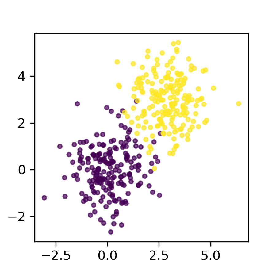
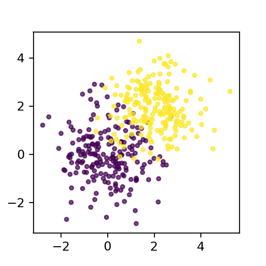
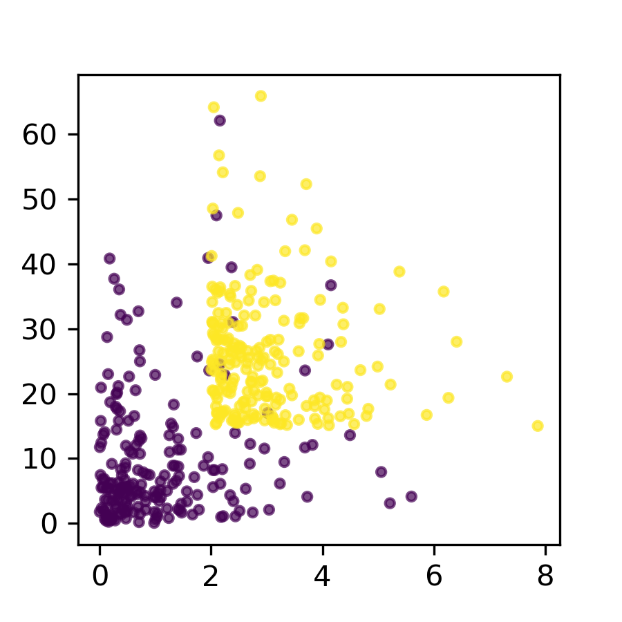
Since most clustering approaches are based on a single view, we first compare our model with them using simulations. For a clear visualization, we generate data from the two-component mixture distribution in a single view , with . Figure 8(a-f) plots the generated data under different settings.

and .
and .
and .

and
and

and
For comparison, we test other clustering algorithms, provided by the Scikit-Learn Cluster package. We use the Normalized Mutual Information (NMI) as a benchmark score. NMI measures the accuracy of the estimated cluster labels with respect to the ground truth labels and is invariant to label-switching. The result is listed in Table 1. In the Gaussian cases (a-c), the Gaussian mixture as the true model has the best performance. When the symmetric and Gaussian-tail assumptions are violated (d-f), more recent methods such as spectral clustering start to show their advantage. The performance of the LSP model (with and ) is very close to the spectral clustering; while in (f) with the heavy-tailed distribution creating many ‘outliers’, the spectral clustering fails completely due to the large noise in the raw similarity matrix, and LSP does not have this issue thanks to the low-rank smoothing.
| (a) | (b) | (c) | (d) | (e) | (f) | |
|---|---|---|---|---|---|---|
| K-means | 1 | 0.89 | 0.68 | 0.56 | 0.25 | 0 |
| Affinity propagation | 0.57 | 0.37 | 0.30 | 0.31 | 0.30 | 0.23 |
| Mean-shift | 1 | 0.89 | 0.70 | 0.56 | 0.40 | 0.05 |
| Agglomerative clustering | 1 | 0.77 | 0.62 | 0.54 | 0.17 | 0 |
| DBSCAN | 0.92 | 0 | 0.01 | 0 | 0.43 | 0 |
| OPTICS | 0.23 | 0.20 | 0.17 | 0.21 | 0.19 | 0.17 |
| Gaussian mixture | 1 | 0.91 | 0.70 | 0.58 | 0.37 | 0 |
| Birch | 0.99 | 0.70 | 0.49 | 0.41 | 0.27 | 0.01 |
| Spectral clustering | 1 | 0.89 | 0.70 | 0.59 | 0.55 | 0.0 |
| LSP | 1 | 0.89 | 0.70 | 0.59 | 0.58 | 0.42 |
For uncertainty quantification, we compute the co-assignment probability using the ground truth distribution and compare it with the estimated from the LSP model. The raw and estimated are provided in the appendix. The median absolute deviations (MAD) between and the oracle are , , , , and . In addition, to assess the limitation of the LSP model (and similarity-based algorithms in general), we modify (c) and make the two clusters closer. When two clusters are generated from and , the LSP model could only discover one large cluster. This is not surprising since heavily overlapped clusters can be alternatively taken as one cluster; in such cases, mixture models with stronger assumptions would work better, such as the ones with a parametric density for each cluster.
5.2 Multi View Experiments
5.2.1 Scaling to a large number of views
We first use a simulation to assess the multi-view clustering performance, under a large . We use views, where each view has . To produce distinct clustering patterns, we simulate different ’s, with each row generated from a Dirichlet distribution in a -element simplex; for a better visualization, the rows are re-ordered and grouped by the index (the most probable cluster). Then in each view, we randomly choose one of the five matrices (denoting the choice by ) as the parameterization, and sample the cluster labels . Lastly, we generate each data point , with , and , so that there is moderate overlap between clusters. Figure 10(a) plots five similarity matrices representative for those distinct patterns.


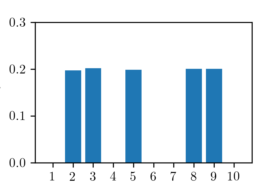
When fitting the LSP model, we use . To examine the quality of initialization, we compare the initialized and the oracle : they show a high NMI at , indicating that that the K-means on the log-odds of ’s gives a very good initialization. After running the EM algorithm, we do see of the estimated ’s are shrunk to near zero [Figure 10(c)], and the estimated ’s with non-trivial ’s indeed recover the five patterns [Figure 10(b)]. For these high dimensional data, the algorithm takes about 10 minutes to finish on a CUDA GPU with 11Gb of memory.
5.2.2 Clustering UCI Hand Written Digits
Since the software is not readily available for most of the existing multi-view clustering methods, we use a dataset that was previously used for benchmark and reported by Kumar et al. 2011. The dataset is the UCI Dutch utility maps handwritten digits data (https://archive.ics.uci.edu/ml/datasets/Multiple+Features), and does not require specific data processing; hence it can provide a fair comparison. The data have six views: (1) 76 Fourier coefficients of the character shapes, (2) 216 profile correlations, (3) 64 Karhunen-Loève coefficients, (4) 240-pixel averages in 2 3 windows, (5) Zernike moments and (6) 6 morphological features. For each digit, there are samples; the NMI is calculated as an evaluating criterion.
We compare our model with two other methods: using single-view spectral clustering independently in each view (SV-SC), and co-regularized spectral clustering (C-SC) (Kumar et al. 2011). When fitting the LSP model,we use as its possible max value, and as the known ground truth. The model converges to effective parameterizations: for and .
| Single View | 1 | 2 | 3 | 4 | 5 | 6 |
|---|---|---|---|---|---|---|
| SV-SC | 0.571 | 0.618 | 0.646 | 0.635 | 0.523 | 0.474 |
| LSP | 0.697 | 0.706 | 0.697 | 0.705 | 0.705 | 0.474 |
| Combining Multiple Views | |
|---|---|
| SV-SC (feature concat) | 0.619 |
| C-SC | 0.768 |
| LSP consensus | 0.742 |


We first compute the point estimates under each view. Table 2 shows that, compared to SV-SC, our model produces higher NMI in almost every view (except for the th view). This is likely due to the sharing of information among the first few views in the LSP model. Then we combine views to produce a consensus. LSP has a better performance than using SV-SC on the concatenated features from all views, while it is slightly worse compared to C-SC. On the other hand, LSP has a unique advantage in the uncertainty quantification for each view. As shown in Figure 11, in the first parameterization, the main source of uncertainty is due to the overlap between the st and the th clusters; whereas the second parameterization has larger overlap among clusters and .
5.2.3 Clustering Brains via RNA-Sequencing Data
We now consider a scientific application with the RNA Sequencing data originated from the human aging, dementia, and traumatic brain injury (TBI) study. The data are obtained from the Allen Institute for Brain Science (Miller et al. 2017) (https://aging.brain-map.org/download/index), and the hippocampus region is chosen for its important role in aging-related disease. Among the brains, there are containing gene expression data in the hippocampus. The age of the subjects at death has an average of and a standard deviation of . There are genes, each with normalized gene-level FPKM values. Since most of the genes contain very little discriminability, a screening step is first carried out: the genes are ranked by their standard deviation divided by the median, with the top chosen for the downstream modeling.
This experiment treats each gene as a view, and clusters the brains using the gene expression. The LSP model was initialized at and . It converges to effective latent parameterizations and at most non-trivial clusters.
For validation, the multi-view results are compared against observed clinical covariates — such as sex, whether had TBI before, dementia evaluation scores, etc. For each clinical covariate, the NMIs are computed by comparing it against the estimated for . To see if there is a possible link between the gene(s) and clinical covariates, for each covariate, we take the maximum of NMIs (MaxNMI) and plot it in Figure 12(a). As this involves multiple comparisons, to show the findings are unlikely to be false positives, we consider two additional baseline MaxNMIs: 1) we randomly draw Bernoulli random vectors, each of length , and compute the MaxNMI to each covariate. We repeat the simulation with different Bernoulli probabilities (ranging from to , the largest MaxNMI is ; 2) it was previously reported in a meta-analysis study (Tan et al. 2016), that the difference in the covariate sex has no clear effect on the hippocampus area, in our experiment, it has MaxNMI . Therefore, we choose MaxNMI as a cut-off. For clarification, these results are mainly exploratory due to the small ; more data are needed before making any statistical claims.
Among all the covariates, the CERAD score (measuring the progression of Alzheimer’s disease), the Braak stage (measuring the progression of Parkinson’s disease and Alzheimer’s disease) and the confirmed diagnose of Alzheimer’s disease appear linked to a subset of gene expression. For the covariates seemingly less relevant to gene expression, the length of education also shows large MaxNMI, whereas the experience of traumatic brain injury (TBI), aging and dementia-related score show surprisingly low NMIs. Besides the MaxNMI, Figure 12(b) plots the NMIs of the top 100 genes associated with the selected four covariates. Clearly, each covariate seems more correlated with a distinct set of views/genes.


6 Discussion
In this article, we propose a method to directly estimate the cluster assignment probabilities for each data under multiple views. There are several interesting extensions that could be pursued. 1) The similarity matrix can be computationally prohibitive to handle when is large; therefore, a random feature map (Rahimi and Recht 2008) can be considered. A similar solution has recently been proposed for spectral clustering using random binning features (Wu et al. 2018). 2) We have assumed the views are given; in practice, if they are not known, we could use some domain-specific knowledge to estimate views. For example, in image processing, we could use edge detection and convolution of pixels to form each view. It is useful to study how they would impact the clustering results. 3) It is interesting to combine the LSP model with another loss function such as the one from a regression task, as an extension to our PAC-Bayes theory result. This could create generalized Bayes models and form new insights about the semi-supervised learning.
Appendix A Proof of the main theorem
Proof 1
Let be the Kullbeck-Leibler divergence between two generating distributions for a cluster graph using or as the co-assignment probability matrix. The sample space of the distribution is a sub-space subject to constraints described in (11). We assume that is given.
Step 1. Change of measure:
where the first equality is because ’s are iid, the first inequality uses the convexity of the function; the second inequality uses the change of measure inequality [Lemma 4 in (Seldin and Tishby 2010)].
Due to the Markov’s inequality, with probability greater than ,
and the last equality is due to is upper bounded, hence we can use Fubini’s theorem.
Step 2. Bounding the exponential function by a constant:
Using Theorem 1 of (Maurer 2004),
Step 3. Relaxing the KL-divergences between two cluster graph distributions to total element-wise divergences:
where the inequality is due to the non-negativity of each function and .
Combining the results,
Taking , summing both sides over and dividing by yields the result.
Appendix B Single View Simulation


References
- Arthur and Vassilvitskii (2007) Arthur, D. and S. Vassilvitskii (2007). K-means++: the advantages of careful seeding. In Proceedings of the 18th annual ACM-SIAM symposium on Discrete algorithms, pp. 1027–1035. Society for Industrial and Applied Mathematics.
- Blei and Frazier (2011) Blei, D. M. and P. I. Frazier (2011). Distance dependent Chinese restaurant processes. Journal of Machine Learning Research 12(Aug), 2461–2488.
- Dahl et al. (2017) Dahl, D. B., R. Day, and J. W. Tsai (2017). Random partition distribution indexed by pairwise information. Journal of the American Statistical Association 112(518), 721–732.
- Dilokthanakul et al. (2016) Dilokthanakul, N., P. A. Mediano, M. Garnelo, M. C. Lee, H. Salimbeni, K. Arulkumaran, and M. Shanahan (2016). Deep unsupervised clustering with Gaussian mixture variational autoencoders. arXiv preprint arXiv:1611.02648.
- Duan and Dunson (2018) Duan, L. L. and D. B. Dunson (2018). Bayesian distance clustering. arXiv preprint arXiv:1810.08537.
- El Moselhy and Marzouk (2012) El Moselhy, T. A. and Y. M. Marzouk (2012). Bayesian inference with optimal maps. Journal of Computational Physics 231(23), 7815–7850.
- Fern and Brodley (2003) Fern, X. Z. and C. E. Brodley (2003). Random projection for high dimensional data clustering: a cluster ensemble approach. In Proceedings of the 20th International Conference on Machine Learning, pp. 186–193.
- Fraley and Raftery (2002) Fraley, C. and A. E. Raftery (2002, June). Model-based clustering, discriminant analysis, and density estimation. Journal of the American Statistical Association 97(458), 611–631.
- Ghahramani and Hinton (1996) Ghahramani, Z. and G. E. Hinton (1996). The EM algorithm for mixtures of factor analyzers. Technical report, Technical Report CRG-TR-96-1, University of Toronto.
- Guan et al. (2010) Guan, Y., J. G. Dy, D. Niu, and Z. Ghahramani (2010). Variational inference for nonparametric multiple clustering. In MultiClust Workshop, Knowledge Discovery and Data Mining.
- Guedj (2019) Guedj, B. (2019). A primer on PAC-bayesian learning. arXiv preprint arXiv:1901.05353.
- Handcock et al. (2007) Handcock, M. S., A. E. Raftery, and J. M. Tantrum (2007). Model-based clustering for social networks. Journal of the Royal Statistical Society: Series A (Statistics in Society) 170(2), 301–354.
- Hennig et al. (2004) Hennig, C. et al. (2004). Breakdown points for maximum likelihood estimators of location–scale mixtures. The Annals of Statistics 32(4), 1313–1340.
- Hoff (2006) Hoff, P. D. (2006). Model-based subspace clustering. Bayesian Analysis 1(2), 321–344.
- Hoff et al. (2002) Hoff, P. D., A. E. Raftery, and M. S. Handcock (2002). Latent space approaches to social network analysis. Journal of the American Statistical Association 97(460), 1090–1098.
- Joshi et al. (2016) Joshi, S., J. Ghosh, M. Reid, and O. Koyejo (2016). Rényi divergence minimization based co-regularized multiview clustering. Machine Learning 104(2-3), 411–439.
- Kingma and Ba (2014) Kingma, D. P. and J. Ba (2014). ADAM: a method for stochastic optimization. In International Conference on Learning Representations, pp. 3455–3463.
- Kirk et al. (2012) Kirk, P., J. E. Griffin, R. S. Savage, Z. Ghahramani, and D. L. Wild (2012). Bayesian correlated clustering to integrate multiple datasets. Bioinformatics 28(24), 3290–3297.
- Kumar et al. (2011) Kumar, A., P. Rai, and H. Daume (2011). Co-regularized multi-view spectral clustering. In Advances in Neural Information Processing Systems, pp. 1413–1421.
- Law et al. (2003) Law, M. H., A. K. Jain, and M. Figueiredo (2003). Feature selection in mixture-based clustering. In Advances in Neural Information Processing Systems, pp. 641–648.
- Li and Shafto (2011) Li, D. and P. Shafto (2011). Bayesian hierarchical cross-clustering. In Proceedings of the 14th International Conference on Artificial Intelligence and Statistics, pp. 443–451.
- Lock and Dunson (2013) Lock, E. F. and D. B. Dunson (2013). Bayesian consensus clustering. Bioinformatics 29(20), 2610–2616.
- Maurer (2004) Maurer, A. (2004). A note on the PAC Bayesian theorem. arXiv preprint cs/0411099.
- Meier et al. (2008) Meier, L., S. Van De Geer, and P. Bühlmann (2008). The group lasso for logistic regression. Journal of the Royal Statistical Society: Series B (Statistical Methodology) 70(1), 53–71.
- Miller et al. (2017) Miller, J. A., A. Guillozet-Bongaarts, L. E. Gibbons, N. Postupna, A. Renz, A. E. Beller, S. M. Sunkin, L. Ng, S. E. Rose, and K. A. Smith (2017). Neuropathological and transcriptomic characteristics of the aged brain. Elife 6, e31126.
- Miller and Dunson (2018) Miller, J. W. and D. B. Dunson (2018). Robust Bayesian inference via coarsening. Journal of the American Statistical Association, 1–13.
- Mo et al. (2017) Mo, Q., R. Shen, C. Guo, M. Vannucci, K. S. Chan, and S. G. Hilsenbeck (2017). A fully Bayesian latent variable model for integrative clustering analysis of multi-type omics data. Biostatistics 19(1), 71–86.
- Niu et al. (2012) Niu, D., J. Dy, and Z. Ghahramani (2012). A nonparametric Bayesian model for multiple clustering with overlapping feature views. In Artificial Intelligence and Statistics, pp. 814–822.
- Niu et al. (2010) Niu, D., J. G. Dy, and M. I. Jordan (2010). Multiple non-redundant spectral clustering views. In Proceedings of the 27th International Conference on Machine Learning, pp. 831–838.
- Niu et al. (2013) Niu, D., J. G. Dy, and M. I. Jordan (2013). Iterative discovery of multiple alternative clustering views. IEEE Transactions on Pattern Analysis and Machine Intelligence 36(7), 1340–1353.
- Ohama et al. (2017) Ohama, I., I. Sato, T. Kida, and H. Arimura (2017). On the model shrinkage effect of gamma process edge partition models. In Advances in Neural Information Processing Systems, pp. 397–405.
- Rahimi and Recht (2008) Rahimi, A. and B. Recht (2008). Random features for large-scale kernel machines. In Advances in Neural Information Processing Systems, pp. 1177–1184.
- Rasmussen (2000) Rasmussen, C. E. (2000). The infinite Gaussian mixture model. In Advances in Neural Information Processing Systems, pp. 554–560.
- Seldin and Tishby (2010) Seldin, Y. and N. Tishby (2010). PAC-Bayesian analysis of co-clustering and beyond. Journal of Machine Learning Research 11(Dec), 3595–3646.
- Tadesse et al. (2005) Tadesse, M. G., N. Sha, and M. Vannucci (2005). Bayesian variable selection in clustering high-dimensional data. Journal of the American Statistical Association 100(470), 602–617.
- Tan et al. (2016) Tan, A., W. Ma, A. Vira, D. Marwha, and L. Eliot (2016). The human hippocampus is not sexually-dimorphic: meta-analysis of structural MRI volumes. Neuroimage 124, 350–366.
- Teh et al. (2005) Teh, Y. W., M. I. Jordan, M. J. Beal, and D. M. Blei (2005). Sharing clusters among related groups: hierarchical Dirichlet processes. In Advances in Neural Information Processing Systems, pp. 1385–1392.
- Wade and Ghahramani (2018) Wade, S. and Z. Ghahramani (2018). Bayesian cluster analysis: point estimation and credible balls. Bayesian Analysis 13(2), 559–626.
- Witten and Tibshirani (2010) Witten, D. M. and R. Tibshirani (2010). A framework for feature selection in clustering. Journal of the American Statistical Association 105(490), 713–726.
- Wu et al. (2018) Wu, L., P.-Y. Chen, I. E.-H. Yen, F. Xu, Y. Xia, and C. Aggarwal (2018). Scalable spectral clustering using random binning features. In Proceedings of the 24th ACM SIGKDD International Conference on Knowledge Discovery and Data Mining, pp. 2506–2515. ACM.
- Yuan and Lin (2006) Yuan, M. and Y. Lin (2006). Model selection and estimation in regression with grouped variables. Journal of the Royal Statistical Society: Series B (Statistical Methodology) 68(1), 49–67.
- Zelnik-Manor and Perona (2005) Zelnik-Manor, L. and P. Perona (2005). Self-tuning spectral clustering. In Advances in Neural Information Processing Systems, pp. 1601–1608.
- Zhou (2014) Zhou, M. (2014). Beta-negative binomial process and exchangeable random partitions for mixed-membership modeling. In Advances in Neural Information Processing Systems, pp. 3455–3463.