A Quantum Annealing-Based Approach to Extreme Clustering

In general, the computational complexity of distance-based clustering methods is proportional to the square of the dataset cardinality, as all pairwise distances must be computed. This bottleneck can be overcome by dividing the dataset and employing distributed approaches balcan2013distributed; malkomes2015fast; har2004coresets, yielding a result different from the one we would obtain when applying clustering methods on the entire dataset. However, its slight imprecision results in a significant computational speed-up.

A partition $\mathcal{P}$ of $X$ is a collection of non-empty disjoint sets $P_{1},\ldots,P_{k}\subset X$ such that $X=\bigcup_{P\in\mathcal{P}}P$. Elements of partitions are typically referred to as blocks, parts, or cells; however, we refer to them as chunks. The partitioning is intended to be homogeneous: every extracted chunk has an equal number of data points (there might be minor differences when the cardinality of the chunk to be divided is odd). The upper bound on the number of points desired in a chunk is referred to as the maximum chunk cardinality $\kappa$. To determine $\kappa$, one should take into account the number of available processors, their data handling capacity, or, in the case of a quantum annealer, the number of fully connected qubits.

To break the data into chunks, we employ a modified version of the well-known “median cut” algorithm, which is frequently used in colour quantization. First, we select an axis of maximum variance. We then bisect the dataset along the selected axis, say $\ell$, at the median $m$ of $\{x^{(1)}_{\ell},\ldots,x^{(n)}_{\ell}\}$ in such a way as to obtain two data chunks $P_{1}$ and $P_{2}$ whose cardinalities differ by at most one (in the case where $n$ is odd) and which satisfy $P_{1}\subseteq\{x\in X:x_{\ell}\leq m\}$ and $P_{2}\subseteq\{x\in X:x_{\ell}\geq m\}$. We cannot simply assign $P_{1}=\{x\in X:x_{\ell}\leq m\}$ and $P_{2}=X\setminus P_{1}$, as these sets might differ drastically in cardinality. For example, when $x_{\ell}^{(1)}=\ldots=x_{\ell}^{(n)}$, this assignment would imply that $P_{1}=X$ and $P_{2}=\emptyset$.

By using $P_{1}$ and $P_{2}$ in the role of $X$, this process can be repeated iteratively, until the number of data points in the chunk to be divided is less than or equal to the maximum chunk cardinality $\kappa$, yielding a binary tree of data chunks. After $s$ iterations, this leaves us with $2^{s}$ chunks $P^{(s)}_{k}$ such that $X=\bigcup_{1\leq k\leq 2^{s}}P^{(s)}_{k},$ where the union is disjoint. Figure 1 provides a visualization.

The goal of a data coarsening step is, for each chunk, to find representative data points such that their union can replace the original point cloud, while maintaining the original data distribution as accurately as possible.

Let $P=\{x^{(1)},\ldots,x^{(n)}\}$ be a chunk and $\varepsilon>0$ be the radius of interest. In what follows, we assume that all the data points are pairwise different. Practically, this can be achieved by removing duplicates and cumulatively incrementing the weight of the representative point we wish to keep by the weight of the discarded duplicates. The radius of interest $\varepsilon$ induces a weighted graph $G^{\varepsilon}=(P,E^{\varepsilon},w_{P})$, where $P$ is the vertex set, the edge set $E^{\varepsilon}$ is given by the relation $\sim_{\varepsilon}$ defined by $x\sim_{\varepsilon}y$ if and only if $d(x,y)<\varepsilon$ for all $x,y\in P$, and the weight function $w_{P}:P\rightarrow\mathbb{R}_{+}$ is the restriction of $w$ to $P$. For each data point $x^{(i)}$, we denote its weight $w_{P}(x^{(i)})$ by $w_{i}$.

For each data point $x^{(i)}$, we introduce a binary decision variable $s_{i}$ that encodes whether $x^{(i)}$ is used in a possible set $S^{*}$. Furthermore, we define the neighbourhood matrix $N^{(\varepsilon)}$ (or similarity matrix) of the graph $G^{\varepsilon}=(P,E^{\varepsilon},w_{P})$ by $N_{ij}^{(\varepsilon)}=1$ if $x^{(i)}\sim_{\varepsilon}x^{(j)}$, and $N_{ij}^{(\varepsilon)}=0$ otherwise. Problem Equation P0 can then be posed as a quadratically constrained quadratic program (QCQP) given by

Here, the inner summation of the constraint does not need to run over all indices, due to the symmetry of $N^{(\varepsilon)}$. The matrix form of Equation P1 is given by maximizing $s^{T}w$ subject to the constraint $s^{T}\overline{N}^{(\varepsilon)}s=0$, where $\overline{N}^{(\varepsilon)}$ is the upper triangular matrix of $N^{(\varepsilon)}$ having all zeroes along the diagonal. As explained in Section 3.6, Equation P1 is equivalent to the NP-hard MWIS problem for $G^{\varepsilon}=(P,E^{\varepsilon},w_{P})$, and thus is computationally intractable for large problem sizes. Note that Equation P1 can be written as the 0–1 integer linear program (ILP)

Having identified a maximal $\varepsilon$-separated subset $S\subseteq P$, we collapse the vertices $P\setminus S$ into $S$, meaning we update the weight of each $x\in S$ according to the weights of all $y\in P\setminus S$ that satisfy $x\sim_{\varepsilon}y$. We aim to assign each $y\in P\setminus S$ to a unique $x\in S$ by generating a so-called Voronoi decomposition (depicted in Figure 1) of each chunk $P$, which is a partition, where each point $x\in P$ is assigned to the closest point within a subset $S$. More precisely, we define the sets $C_{x}$ as in Equation 1, for each $x\in S$. By construction, $C_{x}$ contains all vertices that will be collapsed into $x$, in particular, $x$ itself. We then assign the coarsened chunk $S$ a new weight function $w_{S}$ defined by

In practice, to prevent having very large values for the individual weights, one might wish to add a linear or logarithmic scaling to this weight assignment. In our experiments, we did not add such a scaling.

BiDViT repeats the procedure of data partitioning, chunk coarsening, and chunk collapsing with an increasing radius of interest, until the entire dataset collapses to a single data point. We call these iterations BiDViT levels. The increase of $\varepsilon$ between BiDViT levels is realized by multiplying $\varepsilon$ by a constant factor, denoted by $\alpha$ and specified by the user. In our implementation we have introduced a node class that has three attributes: coordinates, weight, and parents. We initialize BiDViT by creating a node_list containing the nodes corresponding to the weighted dataset (if no weights are provided then the weights are assumed to be the multiplicity of the data points). After each iteration, we remove the nodes that collapsed into representative nodes from the node_list and keep only the remaining representative nodes. However, we append the removed nodes to the parents of the representative node. The final node_list is a data tree, that is, it consists of only one node, and we can move upwards in the hierarchy by accessing its parents (and their parents and so on); see Figure 2. Two leaves of the data tree share a label with respect to a specific BiDViT level, say $m$, if they have collapsed into centroids which, possibly after multiple iterations, have collapsed into the same centroid at the $m$-th level of the tree. For the sake of reproducibility, we provide pseudocode (see Algorithm 2).

It is worth noting that, at each level, instead of proceeding with the identified representative data points, one can use the cluster centroids, allowing more-accurate data coarsening and label assignment.

Our analysis shows that every interation of the heuristic version of BiDViT has a computational complexity of $\text{O}(dn\log(n/\kappa)+dn\kappa)$. Note that $\kappa\ll n$.

The order of complexity of the partitioning procedure is $\text{O}(dn\log(n/\kappa))$. To see this, note that there are at most $\lceil\log_{2}(n/\kappa)\rceil$ partitioning stages and in the $s$-th stage we split $2^{s-1}$ chunks $P_{i}$, where $i=1,\ldots,2^{s-1}$. Let $n_{i}$ denote the number of data points in chunk $P_{i}$. Finding the dimension of maximum variance has a complexity of $\text{O}(dn_{i})$ and determining the median of this dimension can be achieved in $\text{O}(n_{i})$ via the “median of medians” algorithm. Having computed the median, one can construct two chunks of equal size in linear time. Since $\sum_{1\leq i\leq 2^{s-1}}n_{i}=n$, a partitioning step is $\text{O}(dn\log(n/\kappa))$. Any division of a chunk is independent of the other chunks at a given stage; thus, this procedure can benefit from distributed computing.

The order of complexity for the collapsing process is $\text{O}(dn\kappa)$, as computing the neighbourhood matrix of a chunk is $\text{O}(d\kappa^{2})$ and the heuristic selection procedure is $\text{O}(\kappa^{2})$. The number of chunks is bounded from above by $\lceil n/\kappa\rceil$. This yields a complexity of $\text{O}((n/\kappa)(d\kappa^{2}+\kappa^{2}))=\text{O}(dn\kappa)$. As data coarsening in each chunk is independent, with $\lceil n/\kappa\rceil$ parallel processors available the complexity reduces to $\text{O}(d\kappa^{2})$.

The process of identifying a maximal $\varepsilon$-separated set of maximum weight is equivalent to solving the MWIS problem for the weighted graph $G^{\varepsilon}=(P,E^{\varepsilon},w_{P})$. Let $G=(V,E,w)$ be a weighted graph. A set of vertices $S\subseteq V$ is called independent in $G$ if no two of its vertices are adjacent or, equivalently, if $S$ is a clique in the complement graph. This corresponds to the separation constraint mentioned earlier, where two vertices are adjacent whenever they are less than a distance of $\varepsilon$ apart. The MWIS problem can be expressed as

and is NP-complete for a general weighted graph karp1972reducibility, yet, for specific graphs, there exist polynomial-time algorithms mandal2006maximum; kohler2016linear. Note that the QUBO formulation of the MWIS problem in abbott2018hybrid; hernandez2016novel is related to the one in Equation P4.

If all weights are positive, a maximum weighted independent set is necessarily a maximal independent set. A maximal independent set is a dominating set, that is, a subset $S$ of $V$ such that every $v\in V\setminus S$ is adjacent to some $w\in S$. This corresponds to our observation that every maximal $\varepsilon$-separated subset is $\varepsilon$-dense.

Although BiDViT has been specifically designed for extreme clustering, it yields accurate assignments for low values of $k$. Figure 3 shows the clustering assignment of BiDViT on the 2D grid dataset and on MNIST. The results are obtained by manually selecting a BiDViT level. In the grid dataset, every cluster is identified correctly. In the MNIST dataset, all clusters are recognized, except one. However, as our algorithm is based on metric balls, and some datasets might not conform to such categorization, there are datasets for which it cannot accurately assign clusters. This is true for most clustering algorithms, as they are able to recognize only specific shapes.

To evaluate the performance of BiDViT on high-dimensional datasets in the extreme clustering range, we used the Calinski–Harabasz score calinski1974dendrite and the Davies–Bouldin score davies1979cluster. These clustering metrics are internal evaluation schemes, that is, their values depend solely on the clustered data, not requiring the ground truth label assignment for the dataset. Such schemes must be viewed as heuristic methods: their optimal values do not guarantee optimal clusters but provide a reasonable measure of clustering quality. Detailed analyses have been conducted on the advantages and shortcomings of internal clustering measures liu2010understanding; jain2008innovation. In the extreme clustering scenario, where the objective is to obtain an accurate approximation of the entire dataset instead of categorizing its elements, no true labels are given and thus external evaluation schemes (ones based on the distance to a ground truth clustering assignment) do not qualify as success measures.

Let $C_{1},\ldots,C_{n_{\text{c}}}$ denote a total of $n_{\text{c}}$ detected clusters within a dataset $X$ with $n$ data points. The Calinski–Harabasz score $\mathcal{S}_{\text{CH}}$ of a clustering is defined as a weighted ratio of the inter-cluster squared deviations to the sum of the intra-cluster squared deviations. More precisely, $\mathcal{S}_{\text{CH}}$ is given by

where $c_{k}$, for $k=1,\ldots,n_{\text{c}}$ are the cluster centroids, and $c$ is their mean. High values of $\mathcal{S}_{\text{CH}}$ are indicative of a high clustering quality. The Davies–Bouldin score $\mathcal{S}_{\text{DB}}$ is the average maximum value of the ratios of the pairwise sums of the intra-cluster deviation to the inter-cluster deviation. The score is defined as

where $S_{i}=\sum_{x\in C_{i}}\|x-c_{i}\|/|C_{i}|.$ Low values of $\mathcal{S}_{\text{DB}}$ indicate accurate clustering.

Figure 4 shows $\mathcal{S}_{\text{CH}}$ and $\mathcal{S}_{\text{DB}}$ of clustering assignments obtained with BiDViT and Mini Batch $k$-means clustering sculley2010web for different values of $k$ on the Covertype dataset. Due to their high computational complexity with respect to $k$, many common clustering algorithms could not be applied. Remarkably, $\mathcal{S}_{\text{CH}}$ values are quite similar, indicating that the cluster assignments generated by BiDViT are of comparable quality even though the runtime of our algorithm is significantly shorter. For $\mathcal{S}_{\text{DB}}$, our algorithm outperforms the others for lower values of $k$, and is comparable for large values. One explanation for the slightly weaker performance of BiDViT with respect to $\mathcal{S}_{\text{CH}}$ is that BiDViT aims to minimize the non-squared distances, whereas $\mathcal{S}_{\text{CH}}$ rewards clustering methods that minimize squared distances. Similarly, this explains BiDViT’s advantage for $\mathcal{S}_{\text{DB}}$.

In our experiments, we observed that, with respect to the total runtime, even the heuristic version of BiDViT restricted to a single core outperforms common clustering methods in the extreme clustering domain. Figure 5 shows the runtime required by different clustering algorithms for the Covertype dataset. For the implementation of methods other than BiDViT, we used the publicly available sklearn.clustering module for Python. To generate the plots, we ran the entire BiDViT procedure, then applied classical algorithms for the same values of $k$. The results suggest that, in the extreme clustering domain, the runtime of BiDViT is an order of magnitude faster than that of the agglomerative methods against which it was compared, and multiple orders of magnitude faster than that of $k$-means and Mini Batch $k$-means clustering. The dataset cardinality was restricted to 20,000 points to obtain results for other methods, whereas BiDViT is capable of handling the entire dataset comprising 581,000 points.

We then compared the runtime of BiDViT to PERCH (“Purity Enhancing Rotations for Cluster Hierarchies”), a hierarchical algorithm for extreme clustering kobren2017hierarchical, to our knowledge the only other algorithm designed to solve extreme clustering problems. We restricted both algorithms to using a single core. Table 1 shows that BiDViT performs an order of magnitude faster than PERCH. However, they solve somewhat different problems: whereas BiDViT aims to gradually coarsen a dataset by finding $\varepsilon$-separated, $\varepsilon$-dense subsets, PERCH maximizes the dendrogram purity, a measure of the clustering tree’s consistency kobren2017hierarchical. The clustering tree generated by PERCH is binary and thus enormous, allowing for much finer incremental distinctions between clustering assignments. In contrast, the tree generated by BiDViT is more compact, as multiple data points can collapse into the same representative point. When comparing dendrogram purities, we expect PERCH to outperform BiDViT; when comparing Davies–Bouldin scores at a given level, we expect the opposite. We did not test these hypotheses, as dendrogram purity is an external evaluation scheme, that is, it requires a clustering assignment to use for comparison, which is not available in unsupervised machine learning.

We tested a prototype of BiDViT on a D-Wave 2000Q quantum annealer, a machine that has 2048 qubits and 5600 couplers. According to D-Wave Systems, the computer uses 128,000 Josephson junctions and was the most complex superconducting integrated circuit built to date when introduced in January of 2017 DWave.

Before solving the QUBO problems, we applied preprocessing techniques, reducing their size and difficulty glover2018logical. This proved effective and eliminated a great many variables. In most cases, we observed a size reduction of over 60%.

For the quantum version of BiDViT, we observed higher-quality solutions and a significant speed-up for BiDViT, when compared to common clustering methods. Both observations are based on results shown in Figure 6.

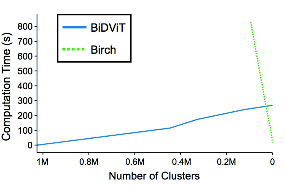
However, the heuristic version of BiDViT and the common clustering algorithms were executed on a classical device that has a limited computational capacity, whereas the D-Wave 2000Q is a highly specialized device. Running these algorithms on a high-performance computer might lead to an equivalent degree of speed-up.

References

- (1) Abbott, A.A., Calude, C.S., Dinneen, M.J., Hua, R.: A Hybrid Quantum-Classical Paradigm to Mitigate Embedding Costs in Quantum Annealing. arXiv:1803.04340 (2018)
- (2) Arthur, D., Vassilvitskii, S.: k-means++: The advantages of careful seeding. In: Proceedings of the eighteenth annual ACM-SIAM symposium on Discrete algorithms. pp. 1027–1035. SIAM (2007)
- (3) Balaji, S., Swaminathan, V., Kannan, K.: Approximating Maximum Weighted Independent Set Using Vertex Support. International Journal of Computational and Mathemtical Sciences 3(8), 406–411 (2009)
- (4) Balcan, M.F., Ehrlich, S., Liang, Y.: Distributed -means and -median clustering on general topologies. In: Adv. Neural Inf. Process. Syst. pp. 1995–2003 (2013)
- (5) Blackard, J.A.: UCI Machine Learning Repository” (2017), http://archive.ics.uci.edu/ml, last accessed 13 Feb. 2019
- (6) Caliński, T., Harabasz, J.: A Dendrite Method for Cluster Analysis. Commun. Stat. Theory Methods 3(1), 1–27 (1974)
- (7) D-Wave Systems Inc. : The D-Wave 2000Q Quantum Computer: Technology Overview (2017), https://www.dwavesys.com/sites/default/files/D-Wave%202000Q%20Tech%20Collateral˙0117F.pdf, last accessed 13 Feb. 2019
- (8) Davies, D.L., Bouldin, D.W.: A Cluster Separation Measure. IEEE Transactions on Pattern Analysis and Machine Intelligence (2), 224–227 (1979)
- (9) Ester, M., Kriegel, H.P., Sander, J., Xu, X., et al.: A density-based algorithm for discovering clusters in large spatial databases with noise. In: KDD. vol. 96, pp. 226–231 (1996)
- (10) Fujitsu Ltd.: Digital Annealer Introduction: Fujitsu Quantum-inspired Computing Digital Annealer (2018), http://www.fujitsu.com/global/documents/digitalannealer/services/da-introduction.pdf, last accessed 13 Feb. 2019
- (11) Glover, F., Lewis, M., Kochenberger, G.: Logical and inequality implications for reducing the size and difficulty of quadratic unconstrained binary optimization problems. European Journal of Operational Research 265(3), 829–842 (2018)
- (12) Har-Peled, S., Mazumdar, S.: On coresets for k-means and k-median clustering. In: Proceedings of the thirty-sixth annual ACM symposium on Theory of computing. pp. 291–300. ACM (2004)
- (13) Hernandez, M., Zaribafiyan, A., Aramon, M., Naghibi, M.: A Novel Graph-Based Approach for Determining Molecular Similarity. arXiv:1601.06693 (2016)
- (14) Hifi, M.: A genetic algorithm-based heuristic for solving the weighted maximum independent set and some equivalent problems. J. Oper. Res. Soc. 48(6), 612–622 (1997)
- (15) Jain, R., Koronios, A.: Innovation in the cluster validating techniques. Fuzzy Optimization and Decision Making 7(3), 233 (2008)
- (16) Kako, A., Ono, T., Hirata, T., Halldórsson, M.: Approximation algorithms for the weighted independent set problem in sparse graphs. Discrete Appl. Math. 157(4), 617–626 (2009)
- (17) Karp, R.M.: Reducibility among Combinatorial Problems. In: Complexity of Computer Computations, pp. 85–103. Springer (1972)
- (18) Kobren, A., Monath, N., Krishnamurthy, A., McCallum, A.: A Hierarchical Algorithm for Extreme Clustering. In: Proceedings of the 23rd ACM SIGKDD International Conference on Knowledge Discovery and Data Mining. pp. 255–264. ACM (2017)
- (19) Köhler, E., Mouatadid, L.: A linear time algorithm to compute a maximum weighted independent set on cocomparability graphs. Inf. Process. Lett. 116(6), 391–395 (2016)
- (20) Kumar, V., Bass, G., Tomlin, C., Dulny, J.: Quantum annealing for combinatorial clustering. Quantum Inf Process 17(2), 39 (2018)
- (21) Kurihara, K., Tanaka, S., Miyashita, S.: Quantum Annealing for Clustering. arXiv:1408.2035 (2014)
- (22) LeCun, Y., Cortes, C., Burges, C.J.: MNIST handwritten digit database. AT&T Labs [Online]. Available: http://yann.lecun.com/exdb/mnist (2010)
- (23) Liu, T., Rosenberg, C., Rowley, H.A.: Clustering Billions of Images with Large Scale Nearest Neighbor Search. In: Proceedings of the 8th IEEE Workshop on Applications of Computer Vision. pp. 28–. WACV ’07, IEEE Computer Society, Washington, DC, USA (2007)
- (24) Liu, Y., Li, Z., Xiong, H., Gao, X., Wu, J.: Understanding of Internal Clustering Validation Measures. In: 2010 IEEE International Conference on Data Mining. pp. 911–916 (2010)
- (25) Lü, Z., Glover, F., Hao, J.K.: A hybrid metaheuristic approach to solving the UBQP problem. European Journal of Operational Research 207(3), 1254–1262 (2010)
- (26) Lucas, A.: Ising formulations of many NP problems. Front. Phys. 2, 5 (2014)
- (27) Maaten, L.v.d., Hinton, G.: Visualizing Data using t-SNE. Journal of Machine Learning Research 9, 2579–2605 (2008)
- (28) Malkomes, G., Kusner, M.J., Chen, W., Weinberger, K.Q., Moseley, B.: Fast distributed k-center clustering with outliers on massive data. In: Advances in Neural Information Processing Systems. pp. 1063–1071 (2015)
- (29) Mandal, S., Pal, M.: Maximum weight independent set of circular-arc graph and its application. J. Appl. Math. Comput. 22(3), 161–174 (2006)
- (30) Merendino, S., Celebi, M.E.: A Simulated Annealing Clustering Algorithm Based On Center Perturbation Using Gaussian Mutation. In: The 26th International FLAIRS Conference (2013)
- (31) Nayak, R., Mills, R., De-Vries, C., Geva, S.: Clustering and Labeling a Web Scale Document Collection using Wikipedia clusters. In: Proceedings of the 5th International Workshop on Web-scale Knowledge Representation Retrieval & Reasoning. pp. 23–30. ACM (2014)
- (32) Nolte, A., Schrader, R.: A note on the finite time behavior of simulated annealing. Mathematics of Operations Research 25(3), 476–484 (2000)
- (33) Sculley, D.: Web-scale k-means clustering. In: Proceedings of the 19th International Conference on World Wide Web. pp. 1177–1178. ACM (2010)
- (34) de Vries, C.M., de Vine, L., Geva, S., Nayak, R.: Parallel Streaming Signature EM-tree: A Clustering Algorithm for Web Scale Applications. In: Proceedings of the 24th International Conference on World Wide Web. pp. 216–226. International World Wide Web Conferences Steering Committee (2015)
- (35) Wang, X.J., Zhang, L., Liu, C.: Duplicate Discovery on 2 Billion Internet Images. In: Proceedings of the IEEE Conference on Computer Vision and Pattern Recognition Workshops. pp. 429–436 (2013)
- (36) Woodley, A., Tang, L.X., Geva, S., Nayak, R., Chappell, T.: Parallel K-Tree: A multicore, multinode solution to extreme clustering. Future Generation Computer Systems (2018)
- (37) Zhang, T., Ramakrishnan, R., Livny, M.: BIRCH: An Efficient Data Clustering Method for Very Large Databases. In: ACM Sigmod Record. vol. 25, pp. 103–114. ACM (1996)
- (38) Zhu, Z., Fang, C., Katzgraber, H.G.: borealis – A generalized global update algorithm for Boolean optimization problems. arXiv:1605.09399 (2016)
Supplementary Information to the Paper, “A Quantum Annealing-Based Approach to Extreme Clustering”
Appendix A: An Alternative Coarsening Method
In certain situations, a user might not want the approximating set to be -separated but instead might be interested in finding an -dense subset with a minimum number of elements, or, more generally, the minimum cost for some cost function . Finding such a set can be realized in a very similar way to the quantum method of BiDViT. In fact, the only modifications needed would be to Section 3.2 in the paper, where we introduce the concept of chunk coarsening.
Let , and let and , for , be defined as in Section 3.2. Analogously to the weight vector , we define a cost vector by for each . The problem of finding an -dense subset of minimum cost can then be expressed as follows: