Impact of an Interfering Node
on Unmanned Aerial Vehicle Communications M. Kim and J. Lee are with the Department of Information and Communication Engineering, Daegu Gyeongbuk Institute of Science and Technology (DGIST), Daegu 42988, South Korea (e-mail: ads5577@dgist.ac.kr, jmnlee@dgist.ac.kr). The material in this paper was presented, in part, at the Global Communications Conference, Abu Dhabi, UAE, Dec. 2018 [1] The corresponding author is J. Lee.

Minsu Kim and Jemin Lee, Member, IEEE

Abstract

Unlike terrestrial communications, UAV (UAV) communications have some advantages such as the LoS (LoS) environment and flexible mobility. However, the interference will be still inevitable. In this paper, we analyze the effect of an interfering node on the UAV communications by considering the LoS probability and different channel fading for LoS and NLoS (NLoS) links, which are affected by horizontal and vertical distances of the communication link. We then derive a closed-form outage probability in the presence of an interfering node for all the possible scenarios and environments of main and interference links. After discussing the impacts of transmitting and interfering node parameters on the outage probability, we show the existence of the optimal height of the UAV that minimizes the outage probability. We also show the NLoS environment can be better than the LoS environment if the average received power of the interference is more dominant than that of the transmitting signal on UAV communications. Finally, we analyze the network outage probability for the case of multiple interfering nodes using stochastic geometry and the outage probability of the single interfering node case, and show the effect of the interfering node density on the optimal height of the UAV.

Index Terms:

Unmanned aerial vehicle, interfering node, air-to-air channel, line-of-sight probability, outage probability

I Introduction

As the UAV technology develops, reliable UAV communications have become necessary. However, since UAV communications are different from conventional terrestrial communications, it is hard to apply the technologies used in terrestrial communications to UAV communications[2, 3, 4, 5]. Especially, unlike terrestrial communications, UAV communications can have LoS environments between a UAV and a ground device, and between UAV. When the main link is in the LoS environment, the received main signal power will increase due to better channel fading and lower path loss exponent compared to the NLoS environment. It also means that in the presence of an interfering node, the interfering signal can be received with larger power as the interfering link can also be in the LoS environment [6, 7].

UAV communications have been studied in the literature, mostly focused on the optimal positioning and trajectory of the UAV. The height of the UAV affects the communication performance in different ways. As the height increases, the UAV forms the LoS link with higher probability, which is modeled by the LoS probability in [8], but the distance to the receiver at the ground increases as well. By considering this relation, the optimal height of the UAV in terms of the communication coverage in the A2G (A2G) channel is presented in [8, 9, 10]. For the case of using a UAV as a relay, the optimal height and position of UAV have also been presented in [11, 12]. The optimal deployment and trajectory of the UAV have been presented to minimize the power consumption in [13, 14]. The height of the UAV and the power allocation factor have been jointly optimized to minimize the hybrid outage probability in [15]. The UAV trajectory and transmit power control have been jointly optimized to minimize the outage probability in [16] and to maximize the average secrecy rate in [17]. The work in [18] jointly optimized the throughput and the access delay using a cyclical multiple access scheme, and the work in [19] jointly optimized the communication time allocation and the UAV trajectory to maximize spectrum efficiency and energy efficiency. However, the works in [17, 16, 18, 19] did not consider the LoS probability, and all of those works analyzed and optimized for the UAV communications in the absence of an interfering node. Since the interference is an inevitable factor in the current and future networks, the impact of the interference on the UAV communications needs to be investigated carefully.

Recently, the interference has been considered in some works such as [20, 21, 22, 23, 24, 25, 26, 27, 28, 29, 30, 31, 32, 33, 34, 35] for the optimal positioning and trajectory of the UAV. The optimal deployment of the UAV has been presented to maximize the communication coverage according to system parameters in [20, 21, 22, 23, 24, 25, 26, 27, 28]. The user scheduling and the UAV trajectory have been jointly optimized to maximize the minimum average rate in [29] and the minimum secrecy rate in [30]. The UAV trajectory is also optimized jointly with the device-UAV association and the uplink power to minimize the total transmit power according to the number of update times in [31]. The random 3D trajectory of the UAV has been presented to maximize the link capacity between the UAV in [32]. The work in [33] proposed an anti-jamming relay strategy for the UAV-aided VANET (VANET). The performance of the UAV communication over the LTE (LTE) network has been analyzed by the measurement and simulation results in [34, 35]. However, all of those prior works considered limited UAV communication scenarios or environments. Specifically, only the path loss is used for channels without fading in [20, 21, 29, 30, 31, 33], or the fact that the LoS probability can be different according to the locations of the UAV was not considered in [22, 32]. In addition, the works in [23, 24, 25, 26, 27, 28] considered the different channel fadings depending on the LoS probability. However, the works in [23, 24, 25, 26, 27] used the path loss exponents and channel fading parameters, which are constant, not changed by the horizontal distance and the vertical distance of the communication link. The work in [28] used the different path loss exponents according to the UAV height, while the channel fading parameters are constant.

TABLE I: Notations used throughout the paper.

Notation	Definition
$i\in\{\text{m},\text{I}\}$	Index for the main link ( $i$ = m) and the interference link ( $i$ = I)
$h_{i}$	Channel fading gain of the link $i$
$\ell_{i}$	Distance of the link $i$
$\mathcal{D}=(\ell_{\text{m}},\ell_{\text{I}})$	Link distance set
$d_{i}^{(\text{H})}$	Horizontal distance of the link $i$
$d_{i}^{(\text{V})}$	Vertical distance of the link $i$
$\alpha(\ell_{i})$	Path loss exponent of the link $i$ for given $\ell_{i}$
$K(\ell_{i})$	Rician factor for given $\ell_{i}$
$p_{\text{L}}(\ell_{i})$	LoS probability for given $\ell_{i}$
$P_{i}$	Transmission power of the link $i$
$N_{\text{o}}$	Noise power
$\gamma(\ell_{\text{m}},\ell_{\text{I}})$	Signal-to-interference-plus-noise ratio (SINR)
$\hat{\gamma}(\ell_{\text{m}},\ell_{\text{I}})$	Signal-to-interference ratio (SIR)
$\gamma_{\text{t}}$	Target SINR/SIR
$e_{i}\in\{\text{L},\text{N}\}$	Index for the LoS environment ( $e_{i}$ = L) and the NLoS environment ( $e_{i}$ = N)
$p_{\text{o}}^{({e_{\text{m}},e_{\text{I}}})}(\mathcal{D})$	Outage probability with the environment of the main link $e_{\text{m}}$ and that of the interference link $e_{\text{I}}$

Therefore, in this paper, we analyze the effect of an interfering node on the UAV communications by considering both the LoS and NLoS links and channel fading. We consider more realistic channel model for UAV communications. Specifically, the probability of forming the LoS link is determined by the heights of the transmitter and the receiver and the horizontal and vertical distances of communication links. Not only the pathloss exponent but also the fading channel factors (e.g., Rician factor) are modeled to be affected by the LoS probability. The main contribution of this paper can be summarized as follows:

•

we consider all possible scenarios of the main (i.e., from a transmitter to a receiver) and the interference (i.e., from an interfering node to a receiver) links on UAV communications, of which channels can be G2A (G2A), G2G (G2G), A2G, or A2A (A2A) channels;
•

we provide the outage probability in the presence of an interfering node for all the scenarios in general environments by considering the LoS probability and different channel fadings for LoS and NLoS links;
•

we derive a closed-form outage probability for the interference-limited environments, and using it, we also figure out whether the LoS environments for both main and interference links can be better than the NLoS environments in terms of the outage probability;
•

we then analyze how the outage probability is affected by the heights of a transmitter and an interfering node and the link distances, and show the optimal UAV heights that minimize the outage probability through numerical results; and
•

we finally present the network outage probability by considering a network with multiple transmitting (also interfering) nodes and a UAV receiver in the air, and show the effect of the transmitting node density on the optimal UAV height.

The remainder of this paper is organized as follows. In Section II, we present the network model and the channel model affected by horizontal and vertical distances of communication links. We then derive a closed-form outage probability for the general environment and the interference-limited environment in Section III. In Section IV, we present the network outage probability considering multiple transmitting (also interfering) nodes. In Section V, we evaluate the performance of UAV communications according to the UAV height, system parameters, and the channel environment. We then compare the optimal UAV heights of the multiple interfering nodes case with that of the single nearest interfering node case. Finally, the conclusion is presented in Section VI.

Notation: The notation used throughout the paper is reported in Table I.

II System Model

In this section, we describe the network model and the channel model on UAV communications.

II-A Terrestrial & Aerial Network Models

We consider a UAV network, which has a UAV, a ground device (e.g., ground control station or base station), and an interfering node. In this network, there can be three types of communications: UAV to UAV, UAV to ground device (or ground device to UAV), and ground device to ground device. The interfering node can be either on the ground or in the air, and we consider one interfering node.¹¹ 1 Note that the result of this paper can be readily extended for the multiple interfering nodes case as presented in Section IV. However, the analysis results will be complicated and give fewer insights. In addition, the communication performance is generally determined by one critical interfering node, especially in low outage probability region [36]. Therefore, we focus on the one interfering node case in this work, but the performance for the multiple interfering nodes case is also presented in simulation results of Section V.

Refer to caption — Fig. 1: System model when UAVs are the communication devices. There are four types of channels: ground-to-ground (G2G), ground-to-air (G2A), air-to-ground (A2G), and air-to-air (A2A) channels. The blue lines represent the main links and the red dotted lines represent the interference links.

When a transmitter (Tx), located at $(x_{\text{m}},y_{\text{m}},z_{\text{m}})$ , communicates to a receiver (Rx), located at $(0,0,z_{\text{o}})$ , in the presence of an interfering node at $(x_{\text{I}},y_{\text{I}},z_{\text{I}})$ , SINR (SINR) is given by

\displaystyle\gamma(\ell_{\text{m}},\ell_{\text{I}})

\displaystyle=\frac{h_{\text{m}}\ell_{\text{m}}^{-\alpha_{\text{m}}(\ell_{\text{m}})}P_{\text{m}}}{h_{\text{I}}\ell_{\text{I}}^{-\alpha_{\text{I}}(\ell_{\text{I}})}P_{\text{I}}+N_{\text{o}}}=\frac{h_{\text{m}}\beta_{\text{m}}(\ell_{\text{m}})}{h_{\text{I}}\beta_{\text{I}}(\ell_{\text{I}})+N_{\text{o}}}

(1)

where $\beta_{\text{m}}(\ell_{\text{m}})$ and $\beta_{\text{I}}(\ell_{\text{I}})$ are respectively given by

\displaystyle\beta_{\text{m}}(\ell_{\text{m}})=\ell_{\text{m}}^{-\alpha_{\text{m}}(\ell_{\text{m}})}P_{\text{m}},\quad\beta_{\text{I}}(\ell_{\text{I}})=\ell_{\text{I}}^{-\alpha_{\text{I}}(\ell_{\text{I}})}P_{\text{I}}.

(2)

Here, $h_{\text{m}}$ and $h_{\text{I}}$ are the fading gains of the main link (i.e., the channel between Tx and Rx) and the interference link (i.e., the channel between interfering node and Rx), respectively; $\ell_{\text{m}}\hskip-1.99168pt=\hskip-1.99168pt\sqrt{x_{\text{m}}^{2}+y_{\text{m}}^{2}+(z_{\text{m}}-z_{\text{o}})^{2}}$ and $\ell_{\text{I}}\hskip-1.99168pt=\hskip-1.99168pt\sqrt{x_{\text{I}}^{2}+y_{\text{I}}^{2}+(z_{\text{I}}-z_{\text{o}})^{2}}$ are the distances of the main link and the interference link, respectively; $P_{\text{m}}$ and $P_{\text{I}}$ are the transmission power of the Tx and the interfering node, respectively; $\alpha_{\text{m}}(\ell_{\text{m}})$ and $\alpha_{\text{I}}(\ell_{\text{I}})$ are the path loss exponents of the main link and the interference link, respectively; and $N_{\text{o}}$ is the noise power. Here, we define that $d_{i}^{(\text{H})}=\sqrt{x_{i}^{2}+y_{i}^{2}}$ is the horizontal distance and $d_{i}^{(\text{V})}=\sqrt{(z_{i}-z_{\text{o}})^{2}}$ is the vertical distance of the main link ( $i=\text{m}$ ) or the interference link ( $i=\text{I}$ ).

II-B Channel Model

As shown in Fig. 1, there are three types of the channels in the UAV networks: the A2G channel (from UAV to a ground device), the A2A channel (from UAV to UAV), and the G2G channel (from a ground device to a ground device). The G2G channel is the same channel of a terrestrial network, which is generally modeled as the NLoS environment with Rayleigh fading in urban areas. The G2A channel and the A2G channel have the same characteristics, so we describe characteristics of the A2G and A2A channels in this subsection.

The A2G and A2A channels can have the LoS or NLoS environment depending on the height of the UAV and its surrounding environment such as buildings. In the following, we describe the channel components affected by the horizontal distance $d_{i}^{(\text{H})}$ and the vertical distance $d_{i}^{(\text{V})}$ , and then provide the models for A2G and A2A channels.

II-B1 Channel components

The horizontal distance $d_{i}^{(\text{H})}$ and the vertical distance $d_{i}^{(\text{V})}$ of the communicatin link affect the probability of forming LoS link, the path loss exponent, and the Rician factor as described below.

•

The LoS probability is given by [37, 38]

		$\displaystyle p_{\text{L}}(\ell_{i})=$		(3)
		$\displaystyle\left\{\begin{aligned} &\left\{1-\exp\left(-\frac{z_{i}^{2}}{2\zeta^{2}}\right)\right\}^{\ell_{i}\sqrt{\nu\mu}}\quad\quad\quad\quad\quad\,\,\,\,\,\text{for}\,\,z_{i}=z_{\text{o}}\\ &\left\{1\hskip-1.42262pt-\hskip-1.42262pt\frac{\sqrt{2\pi}\zeta}{d_{i}^{(\text{V})}}\Bigg\|Q\hskip-2.84526pt\left(\frac{z_{i}}{\zeta}\right)\hskip-2.84526pt-\hskip-1.42262ptQ\hskip-2.84526pt\left(\frac{z_{\text{o}}}{\zeta}\right)\hskip-2.84526pt\Bigg\|\right\}^{d_{i}^{(\text{H})}\hskip-1.42262pt\sqrt{\nu\mu}}\,\,\,\text{for}\,\,z_{i}\neq z_{\text{o}}\end{aligned}\right.$

where $Q(x)=\int_{x}^{\infty}\frac{1}{\sqrt{2\pi}}\exp\left(-\frac{t^{2}}{2}\right)\,dt$ is the Q-function and $\zeta$ , $\nu$ , and $\mu$ are environment parameters, which are determined by the building density and heights of the Tx and the Rx. Furthermore, the NLoS probability is $p_{\text{N}}(\ell_{i})=1-p_{\text{L}}(\ell_{i})$ .

•

The path loss exponent is determined by $\ell_{i}$ as [12]

$\displaystyle\alpha(\ell_{i})=a_{1}p_{\text{L}}(\ell_{i})+b_{1}$ (4)

where $a_{1}=\alpha_{\text{L}}-\alpha_{\text{N}}$ and $b_{1}=\alpha_{\text{N}}$ . Here, $\alpha_{\text{L}}$ and $\alpha_{\text{N}}$ are the path loss exponenets when the LoS probabilities are one and zero, respectively.
•

The Rician factor is proposed to be determined by $\ell_{i}$ as

$\displaystyle K(\ell_{i})=a_{2}\exp\left\{b_{2}p_{\text{L}}(\ell_{i})^{2}\right\}$ (5)

where $a_{2}=K_{\text{N}}$ and $b_{2}=\ln\left(\frac{K_{\text{L}}}{K_{\text{N}}}\right)$ . Here, $K_{\text{L}}$ and $K_{\text{N}}$ are denoted as the Rician factors when the LoS probabilities are one and zero, respectively. Note that the Rician factor, defined by the elevation angle $\theta_{i}$ as $K(\theta_{i})=a_{2}\exp(b_{2}\theta_{i})$ [12], was used in prior works. However, this model has a problem when applied to the A2A channel. For example, due to smaller elevation angle of A2A channel, the Rician factor of the A2A channel becomes smaller than that of the A2G channel. This means the average channel fading gain of the A2A channel is smaller than that of the A2G channel, which is not true in reality. On the other hand, the proposed Rician factor model in (5) is changed according to the respective heights of the receiver and the transmitter as shown in Fig. 2.

Fig. 2: Rician factor $K(\ell_{\text{m}})$ as a function of $d_{\text{m}}^{(\text{H})}$ with $d_{\text{m}}^{(\text{V})}=200m$ .

Figure 2 presents the Rician factors $K(\ell_{\text{m}})$ as a function of the horizontal distance of main link $d_{\text{m}}^{(\text{H})}$ for different values of $z_{\text{o}}$ and $z_{\text{m}}$ , where the Rx is located at $(0,0,z_{\text{o}})$ and the Tx moves from $(0,0,z_{\text{m}})$ to $(x_{\text{m}},y_{\text{m}},z_{\text{m}})$ . From this figure, we can see that the Rician factor decreases with $d_{\text{m}}^{(\text{H})}$ because the LoS probability decreases with $d_{\text{m}}^{(\text{H})}$ . We can also see that the Rician factor of the A2A channel (i.e., $20m-220m$ ) is greater than that of the A2G channel (i.e., $0m-200m$ ) even though the elevation angles of both A2A and A2G channels are the same. In addition, the proposed Rician factor has similar trend to the Rician factor in [12] with the same simulation environment.

Note that from (3)-(5), we can see that $p_{\text{L}}(\ell_{i})$ and $K(\ell_{i})$ are increasing functions of $d_{i}^{(\text{V})}$ and $\alpha(\ell_{i})$ is a decreasing function of $d_{i}^{(\text{V})}$ , so the received power increases as $d_{i}^{(\text{V})}$ increases.

II-B2 Air-to-Ground (A2G) & Air-to-Air (A2A) channels

When the main link and the interference link are A2G or A2A channel, $h_{\text{m}}$ and $h_{\text{I}}$ can be in either the LoS or NLoS environment. We consider that the channel fading is Rician fading for the LoS environment and Rayleigh fading for the NLoS environment. Therefore, the distribution of the channel fading, $h_{i}$ , $i\in\{\text{m},\text{I}\}$ , is given by

\displaystyle f_{h_{i}}(h)=\left\{\begin{aligned} &f_{\text{L}}(h)\quad\quad\text{for \acs{LoS} case}\\ &f_{\text{N}}(h)\quad\quad\text{for \acs{NLoS} case}\end{aligned}\right.

(6)

where $f_{\text{L}}(h)$ and $f_{\text{N}}(h)$ are noncentral Chi-squared and exponential distribution, respectively, and given by

$\displaystyle f_{\text{L}}(h)$	$\displaystyle=\frac{1+K(\ell_{i})}{\overline{H_{\text{L}}}}\exp\left(-K(\ell_{i})-\frac{1+K(\ell_{i})}{\overline{H_{\text{L}}}}h\right)$
	$\displaystyle\quad\times I_{0}\left(2\sqrt{\frac{K(\ell_{i})(1+K(\ell_{i}))}{\overline{H_{\text{L}}}}h}\right)$
	$\displaystyle=\frac{1}{2}\exp\left(-K(\ell_{i})-\frac{h}{2}\right)I_{0}\left(\sqrt{2K(\ell_{i})h}\right)$	(7)
$\displaystyle f_{\text{N}}(h)$	$\displaystyle=\frac{1}{\overline{H_{\text{N}}}}\exp\left(-\frac{h}{\overline{H_{\text{N}}}}\right)=\exp\left(-h\right).$	(8)

Here, $I_{0}(\cdot)$ is the modified Bessel function of the first kind with order zero, and $\overline{H_{\text{L}}}=2+2K(\ell_{i})$ and $\overline{H_{\text{N}}}=1$ are the means of LoS and NLoS channel fading gain, respectively.

$\displaystyle p_{\text{o}}^{(\text{L,L})}(\mathcal{D})$	$\displaystyle=1-\frac{1}{2}\int_{0}^{\infty}Q\left(\sqrt{2K_{\text{m}}(\ell_{\text{m}})},\sqrt{\frac{\gamma_{\text{t}}(\beta_{\text{I}}(\ell_{\text{I}})g+N_{\text{o}})}{\beta_{\text{m}}(\ell_{\text{m}})}}\right)\exp\left(-K_{\text{I}}(\ell_{\text{I}})-\frac{g}{2}\right)I_{0}\left(\sqrt{2K_{\text{I}}(\ell_{\text{I}})g}\right)\,dg$	(11)
$\displaystyle p_{\text{o}}^{(\text{L,N})}(\mathcal{D})$	$\displaystyle=1-Q\left(\sqrt{2K_{\text{m}}(\ell_{\text{m}})},\sqrt{\frac{\gamma_{\text{t}}N_{\text{o}}}{\beta_{\text{m}}(\ell_{\text{m}})}}\right)+\frac{\gamma_{\text{t}}\beta_{\text{I}}(\ell_{\text{I}})}{2\beta_{\text{m}}(\ell_{\text{m}})+\gamma_{\text{t}}\beta_{\text{I}}(\ell_{\text{I}})}\exp\left(\frac{N_{\text{o}}}{\beta_{\text{I}}(\ell_{\text{I}})}-\frac{2K_{\text{m}}(\ell_{\text{m}})\beta_{\text{m}}(\ell_{\text{m}})}{2\beta_{\text{m}}(\ell_{\text{m}})+\gamma_{\text{t}}\beta_{\text{I}}(\ell_{\text{I}})}\right)$
	$\displaystyle\quad\times Q\left(\sqrt{\frac{2\gamma_{\text{t}}K_{\text{m}}(\ell_{\text{m}})\beta_{\text{I}}(\ell_{\text{I}})}{2\beta_{\text{m}}(\ell_{\text{m}})+\gamma_{\text{t}}\beta_{\text{I}}(\ell_{\text{I}})}},\sqrt{\frac{N_{\text{o}}(2\beta_{\text{m}}(\ell_{\text{m}})+\gamma_{\text{t}}\beta_{\text{I}}(\ell_{\text{I}}))}{\beta_{\text{m}}(\ell_{\text{m}})\beta_{\text{I}}(\ell_{\text{I}})}}\right)$	(12)

III Outage Probability Analysis

In this section, we analyze the outage probability of UAV communications by considering various environments of main and interference links. The outage probability is provided for two cases: the general environment in Section III-A and the interference-limited environment in Section III-B.

III-A General Environments

For given the link distance set $\mathcal{D}=(\ell_{\text{m}},\ell_{\text{I}})$ of main and interference links, the outage probability is defined as

\displaystyle p_{\text{o}}(\mathcal{D})=\mathbb{P}[\gamma(\ell_{\text{m}},\ell_{\text{I}})<\gamma_{\text{t}}]

(9)

where $\gamma_{\text{t}}$ is the target SINR or SIR (SIR), which can be defined by $\gamma_{\text{t}}=2\!^{\frac{R_{\text{t}}}{W}}-1$ for the target rate $R_{\text{t}}$ and the bandwidth $W$ [39, 40, 41]. Using (9), the outage probability can be derived from the distribution of the channel fading as follows.

Theorem 1

For given $\mathcal{D}=(\ell_{\text{m}},\ell_{\text{I}})$ , the outage probability $p_{\text{o}}(\mathcal{D})$ can be presented as

$\displaystyle p_{\text{o}}(\mathcal{D})$	$\displaystyle=\sum_{e_{\text{m}},e_{\text{I}}\in\{\text{L},\text{N}\}}p_{e_{\text{m}}}(\ell_{\text{m}})p_{e_{\text{I}}}(\ell_{\text{I}})p_{\text{o}}^{(e_{\text{m}},e_{\text{I}})}(\mathcal{D})$
	$\displaystyle=p_{\text{L}}(\ell_{\text{m}})p_{\text{L}}(\ell_{\text{I}})p_{\text{o}}^{(\text{L,L})}(\mathcal{D})$
	$\displaystyle\quad+p_{\text{L}}(\ell_{\text{m}})p_{\text{N}}(\ell_{\text{I}})p_{\text{o}}^{(\text{L,N})}(\mathcal{D})$
	$\displaystyle\quad+p_{\text{N}}(\ell_{\text{m}})p_{\text{L}}(\ell_{\text{I}})p_{\text{o}}^{(\text{N,L})}(\mathcal{D})$
	$\displaystyle\quad+p_{\text{N}}(\ell_{\text{m}})p_{\text{N}}(\ell_{\text{I}})p_{\text{o}}^{(\text{N,N})}(\mathcal{D})$	(10)

where $p_{\text{o}}^{({e_{\text{m}},e_{\text{I}}})}(\mathcal{D})$ is the outage probability with the environment of the main link $e_{\text{m}}$ and that of the interference link $e_{\text{I}}$ . The environment $e_{i}$ can be either LoS (i.e., $e_{i}=\text{L}$ ) or NLoS (i.e., $e_{i}=\text{N}$ ), and $p_{\text{o}}^{({e_{\text{m}},e_{\text{I}}})}(\mathcal{D})$ for four cases of $({e_{\text{m}},e_{\text{I}}})$ are given as follows:

1.

Case 1 ( $e_{\text{m}}=\text{L}$ and $e_{\text{I}}=\text{L}$ ): $p_{\text{o}}\!^{(\text{L,L})}(\mathcal{D})$ is given by (11).
2.

Case 2 ( $e_{\text{m}}=\text{L}$ and $e_{\text{I}}=\text{N}$ ): $p_{\text{o}}\!^{(\text{L,N})}(\mathcal{D})$ is given by (12).

Case 3 ( $e_{\text{m}}=\text{N}$ and $e_{\text{I}}=\text{L}$ ): $p_{\text{o}}\!^{(\text{N,L})}(\mathcal{D})$ is given by

	$\displaystyle p_{\text{o}}\!^{(\text{N,L})}\hskip-0.85358pt(\mathcal{D})\hskip-1.42262pt$	$\displaystyle=\hskip-1.42262pt1-\frac{\beta_{\text{m}}(\ell_{\text{m}})}{2\gamma_{\text{t}}\beta_{\text{I}}(\ell_{\text{I}})+\beta_{\text{m}}(\ell_{\text{m}})}$
		$\displaystyle\hskip-1.42262pt\quad\times\hskip-1.42262pt\exp\hskip-1.42262pt\left(\hskip-2.84526pt-\frac{\gamma_{\text{t}}N_{\text{o}}}{\beta_{\text{m}}(\hskip-0.85358pt\ell_{\text{m}}\hskip-0.85358pt)}\hskip-1.42262pt-\hskip-1.42262pt\frac{2\gamma_{\text{t}}K_{\text{I}}(\hskip-0.85358pt\ell_{\text{I}}\hskip-0.85358pt)\beta_{\text{I}}(\hskip-0.85358pt\ell_{\text{I}}\hskip-0.85358pt)}{2\gamma_{\text{t}}\beta_{\text{I}}(\hskip-0.85358pt\ell_{\text{I}}\hskip-0.85358pt)\hskip-1.42262pt+\hskip-1.42262pt\beta_{\text{m}}(\hskip-0.85358pt\ell_{\text{m}}\hskip-0.85358pt)}\hskip-2.27621pt\right)\hskip-3.41432pt.\hskip-4.55244pt$		(13)

Case 4 ( $e_{\text{m}}=\text{N}$ and $e_{\text{I}}=\text{N}$ ): $p_{\text{o}}\!^{(\text{N,N})}(\mathcal{D})$ is given by

\displaystyle p_{\text{o}}\!^{(\text{N,N})}\hskip-0.85358pt(\mathcal{D})\hskip-1.42262pt=\hskip-1.42262pt1\hskip-1.42262pt-\hskip-1.42262pt\frac{\beta_{\text{m}}(\ell_{\text{m}})}{\beta_{\text{m}}(\ell_{\text{m}})\hskip-1.70717pt+\hskip-1.70717pt\gamma_{\text{t}}\beta_{\text{I}}(\ell_{\text{I}})}\hskip-1.42262pt\exp\hskip-1.42262pt\left(\hskip-2.84526pt-\frac{\gamma_{\text{t}}N_{\text{o}}}{\beta_{\text{m}}(\ell_{\text{m}})}\hskip-1.42262pt\right)\hskip-2.84526pt.\hskip-4.2679pt

(14)

Proof:

See Appendix -A. ∎

From Theorem 1, we can also obtain the outage probability for different scenarios of UAV communications by changing the values of $(z_{\text{m}},z_{\text{I}},z_{\text{o}})$ . Specifically, when the LoS probabilities of main and interference links increase to one according to the values of $(z_{\text{m}},z_{\text{I}},z_{\text{o}})$ , it is only necessary to consider the outage probability $p_{\text{o}}^{(\text{L,L})}(\mathcal{D})$ in (11).

	$\displaystyle\hat{p}_{\text{o}}\!^{(\text{L,L})}(\mathcal{D})$	$\displaystyle=1-Q\left(\sqrt{\frac{2K_{\text{m}}(\ell_{\text{m}})\beta_{\text{m}}(\ell_{\text{m}})}{\beta_{\text{m}}(\ell_{\text{m}})+\gamma_{\text{t}}\beta_{\text{I}}(\ell_{\text{I}})}},\sqrt{\frac{2\gamma_{\text{t}}K_{\text{I}}(\ell_{\text{I}})\beta_{\text{I}}(\ell_{\text{I}})}{\beta_{\text{m}}(\ell_{\text{m}})+\gamma_{\text{t}}\beta_{\text{I}}(\ell_{\text{I}})}}\right)+\frac{\gamma_{\text{t}}\beta_{\text{I}}(\ell_{\text{I}})}{\beta_{\text{m}}(\ell_{\text{m}})+\gamma_{\text{t}}\beta_{\text{I}}(\ell_{\text{I}})}$
		$\displaystyle\quad\times\exp\left(-\frac{K_{\text{m}}(\ell_{\text{m}})\beta_{\text{m}}(\ell_{\text{m}})+\gamma_{\text{t}}K_{\text{I}}(\ell_{\text{I}})\beta_{\text{I}}(\ell_{\text{I}})}{\beta_{\text{m}}(\ell_{\text{m}})+\gamma_{\text{t}}\beta_{\text{I}}(\ell_{\text{I}})}\right)I_{0}\left(\frac{2\beta_{\text{m}}(\ell_{\text{m}})}{\beta_{\text{m}}(\ell_{\text{m}})+\gamma_{\text{t}}\beta_{\text{I}}(\ell_{\text{I}})}\sqrt{\frac{\gamma_{\text{t}}K_{\text{m}}(\ell_{\text{m}})K_{\text{I}}(\ell_{\text{I}})\beta_{\text{I}}(\ell_{\text{I}})}{\beta_{\text{m}}(\ell_{\text{m}})}}\right)$		(17)

III-B Interference-limited Environments

In this subsection, we provide the outage probability when it is dominantly determined by the received power of the interfering signal, i.e., the interference-limited environment. We provide the outage probability in closed-forms, and they can also provide more insights on the effects of environments parameters on the outage probability.

In the interference-limited environment, the outage probability is defined as

\displaystyle\hat{p}_{\text{o}}(\mathcal{D})=\mathbb{P}[\hat{\gamma}(\ell_{\text{m}},\ell_{\text{I}})<\gamma_{\text{t}}]

(15)

where $\hat{\gamma}(\ell_{\text{m}},\ell_{\text{I}})$ is the SIR, given by

\displaystyle\hat{\gamma}(\ell_{\text{m}},\ell_{\text{I}})

\displaystyle=\frac{h_{\text{m}}\ell_{\text{m}}^{-\alpha_{\text{m}}(\ell_{\text{m}})}P_{\text{m}}}{h_{\text{I}}\ell_{\text{I}}^{-\alpha_{\text{I}}(\ell_{\text{I}})}P_{\text{I}}}=\frac{h_{\text{m}}\beta_{\text{m}}(\ell_{\text{m}})}{h_{\text{I}}\beta_{\text{I}}(\ell_{\text{I}})}.

(16)

The outage probability can be derived by a similar approach in Theorem 1, and provided in the following lemma.

Lemma 1

For given $\mathcal{D}=(\ell_{\text{m}},\ell_{\text{I}})$ , the outage probability $\hat{p}_{\text{o}}(\mathcal{D})$ can be presented as (1) by substituting from $p_{\text{o}}^{({e_{\text{m}},e_{\text{I}}})}(\mathcal{D})$ to $\hat{p}_{\text{o}}^{({e_{\text{m}},e_{\text{I}}})}(\mathcal{D})$ , where $\hat{p}_{\text{o}}^{({e_{\text{m}},e_{\text{I}}})}(\mathcal{D})$ are given as follows:

1.

Case 1 ( $e_{\text{m}}=\text{L}$ and $e_{\text{I}}=\text{L}$ ): $\hat{p}_{\text{o}}\!^{(\text{L,L})}(\mathcal{D})$ is given by (17).

Case 2 ( $e_{\text{m}}=\text{L}$ and $e_{\text{I}}=\text{N}$ ): $\hat{p}_{\text{o}}\!^{(\text{L,N})}(\mathcal{D})$ is given by

	$\displaystyle\hat{p}_{\text{o}}\!^{(\text{L,N})}(\mathcal{D})$	$\displaystyle=\frac{\gamma_{\text{t}}\beta_{\text{I}}(\ell_{\text{I}})}{2\beta_{\text{m}}(\ell_{\text{m}})+\gamma_{\text{t}}\beta_{\text{I}}(\ell_{\text{I}})}$
		$\displaystyle\quad\times\exp\left(-\frac{2K_{\text{m}}(\ell_{\text{m}})\beta_{\text{m}}(\ell_{\text{m}})}{2\beta_{\text{m}}(\ell_{\text{m}})+\gamma_{\text{t}}\beta_{\text{I}}(\ell_{\text{I}})}\right).$		(18)

Case 3 ( $e_{\text{m}}=\text{N}$ and $e_{\text{I}}=\text{L}$ ): $\hat{p}_{\text{o}}\!^{(\text{N,L})}(\mathcal{D})$ is given by

	$\displaystyle\hat{p}_{\text{o}}\!^{(\text{N,L})}(\mathcal{D})$	$\displaystyle=1-\frac{\beta_{\text{m}}(\ell_{\text{m}})}{2\gamma_{\text{t}}\beta_{\text{I}}(\ell_{\text{I}})+\beta_{\text{m}}(\ell_{\text{m}})}$
		$\displaystyle\quad\times\exp\left(-\frac{2\gamma_{\text{t}}K_{\text{I}}(\ell_{\text{I}})\beta_{\text{I}}(\ell_{\text{I}})}{2\gamma_{\text{t}}\beta_{\text{I}}(\ell_{\text{I}})+\beta_{\text{m}}(\ell_{\text{m}})}\right).$		(19)

Case 4 ( $e_{\text{m}}=\text{N}$ and $e_{\text{I}}=\text{N}$ ): $\hat{p}_{\text{o}}\!^{(\text{N,N})}(\mathcal{D})$ is given by

\displaystyle\hat{p}_{\text{o}}\!^{(\text{N,N})}(\mathcal{D})=\frac{\gamma_{\text{t}}\beta_{\text{I}}(\ell_{\text{I}})}{\beta_{\text{m}}(\ell_{\text{m}})+\gamma_{\text{t}}\beta_{\text{I}}(\ell_{\text{I}})}.

(20)

Proof:

See Appendix -B. ∎

From Lemma 1, we can also obtain the outage probability for different scenarios of UAV communications by changing the values of $(z_{\text{m}},z_{\text{I}},z_{\text{o}})$ .

From Theorem 1 and Lemma 1, we can readily know that $p_{\text{o}}\!^{(\text{L,N})}(\mathcal{D})$ (Case 2) cannot be higher than $p_{\text{o}}\!^{(\text{N,L})}(\mathcal{D})$ (Case 3) as Case 2 has stronger main link and weaker interference link than Case 3. However, it is not clear whether the outage probability with LoS environments for both main and interference links (Case 1) can be lower or higher than that with NLoS environments for both main and interference links (Case 4). Hence, we compare $p_{\text{o}}\!^{(\text{L,L})}(\mathcal{D})$ and $p_{\text{o}}\!^{(\text{N,N})}(\mathcal{D})$ , and obtain the following results in Corollary 1.

Corollary 1

According to the ratio of the average received signal power of the main and interference links, i.e., $\frac{\beta_{\text{m}}(\ell_{\text{m}})}{\beta_{\text{I}}(\ell_{\text{I}})}$ , the relation between $\hat{p}_{\text{o}}\!^{(\text{L,L})}(\mathcal{D})$ and $\hat{p}_{\text{o}}\!^{(\text{N,N})}(\mathcal{D})$ is changed as

\displaystyle\left\{\begin{aligned} &\hat{p}_{\text{o}}\!^{(\text{L,L})}(\mathcal{D})>\hat{p}_{\text{o}}\!^{(\text{N,N})}(\mathcal{D}),\,\,\,\,\,\text{for}\,\,\,0<\frac{\beta_{\text{m}}(\ell_{\text{m}})}{\beta_{\text{I}}(\ell_{\text{I}})}<v^{\prime}\\ &\hat{p}_{\text{o}}\!^{(\text{L,L})}(\mathcal{D})<\hat{p}_{\text{o}}\!^{(\text{N,N})}(\mathcal{D}),\,\,\,\,\,\text{for}\,\,\,v^{\prime}<\frac{\beta_{\text{m}}(\ell_{\text{m}})}{\beta_{\text{I}}(\ell_{\text{I}})}<\infty\\ &\hat{p}_{\text{o}}\!^{(\text{L,L})}(\mathcal{D})=\hat{p}_{\text{o}}\!^{(\text{N,N})}(\mathcal{D}),\,\,\,\,\,\text{for}\,\,\,\frac{\beta_{\text{m}}(\ell_{\text{m}})}{\beta_{\text{I}}(\ell_{\text{I}})}=0,\infty,\,\text{or}\ v^{\prime}\hskip-2.84526pt\end{aligned}\right.

(21)

where $v^{\prime}$ ( $0<v^{\prime}<\infty$ ) is the value of $\frac{\beta_{\text{m}}(\ell_{\text{m}})}{\beta_{\text{I}}(\ell_{\text{I}})}$ that makes $\hat{p}_{\text{o}}\!^{(\text{L,L})}(\mathcal{D})=\hat{p}_{\text{o}}\!^{(\text{N,N})}(\mathcal{D})$ .

Proof:

For convenience, we introduce $v=\frac{\beta_{\text{m}}(\ell_{\text{m}})}{\beta_{\text{I}}(\ell_{\text{I}})}$ , and define $A(v)$ and $B(v)$ as

\displaystyle A(v)=\sqrt{\frac{2K_{\text{m}}(\ell_{\text{m}})v}{v+\gamma_{\text{t}}}},\quad B(v)=\sqrt{\frac{2\gamma_{\text{t}}K_{\text{I}}(\ell_{\text{I}})}{v+\gamma_{\text{t}}}}.

(22)

By using (22), $\hat{p}_{\text{o}}\!^{(\text{L,L})}(\mathcal{D})$ in (17) and $\hat{p}_{\text{o}}\!^{(\text{N,N})}(\mathcal{D})$ in (20) can rewrite as functions of $v$ as

$\displaystyle\hat{p}_{\text{o}}\!^{(\text{L,L})}(v)$	$\displaystyle=1-Q\left(A(v),B(v)\right)+\frac{\gamma_{\text{t}}}{v+\gamma_{\text{t}}}$
	$\displaystyle\quad\times\exp\left(-\frac{A(v)^{2}+B(v)^{2}}{2}\right)I_{0}\left(A(v)B(v)\right)$
$\displaystyle\hat{p}_{\text{o}}\!^{(\text{N,N})}(v)$	$\displaystyle=\frac{\gamma_{\text{t}}}{v+\gamma_{\text{t}}}.$	(23)

From (23), we obtain the first derivatives of $\hat{p}_{\text{o}}\!^{(\text{L,L})}(v)$ and $\hat{p}_{\text{o}}\!^{(\text{N,N})}(v)$ according to $v$ , respectively, as

		$\displaystyle\frac{\partial\hat{p}_{\text{o}}\!^{(\text{L,L})}(v)}{\partial v}\hskip-1.42262pt=\hskip-1.42262pt\left(\hat{p}_{\text{o}}\!^{(\text{N,N})}(v)\hskip-1.42262pt-\hskip-1.42262pt1\right)\hskip-1.42262pt\exp\hskip-1.42262pt\left(\hskip-1.42262pt-\frac{A(v)^{2}+B(v)^{2}}{2}\right)\hskip-1.42262ptB(v)$
		$\displaystyle\times\Bigg\{I_{1}\left(A(v)B(v)\right)\frac{\partial A(v)}{\partial v}-I_{0}\left(A(v)B(v)\right)\frac{\partial B(v)}{\partial v}\Bigg\}$
		$\displaystyle+\hat{p}_{\text{o}}\!^{(\text{N,N})}(v)\exp\left(-\frac{A(v)^{2}+B(v)^{2}}{2}\right)A(v)$
		$\displaystyle\times\left\{I_{1}\left(A(v)B(v)\right)\frac{\partial B(v)}{\partial v}-I_{0}\left(A(v)B(v)\right)\frac{\partial A(v)}{\partial v}\right\}$
		$\displaystyle+\hskip-1.42262pt\frac{\partial\hat{p}_{\text{o}}\!^{(\text{N,N})}(v)}{\partial v}\hskip-1.42262pt\exp\hskip-2.27621pt\left(\hskip-2.84526pt-\frac{A(v)^{2}\hskip-1.42262pt+\hskip-1.42262ptB(v)^{2}}{2}\right)\hskip-2.84526ptI_{0}\hskip-1.42262pt\left(A(v)B(v)\right)\hskip-1.42262pt<\hskip-1.42262pt0\hskip-2.84526pt$		(24)

\displaystyle\frac{\partial\hat{p}_{\text{o}}\!^{(\text{N,N})}(v)}{\partial v}=-\frac{\gamma_{\text{t}}}{\left(v+\gamma_{\text{t}}\right)^{2}}<0.

(25)

In (III-B) and (25), the inequalities are obtained since $\exp(v)\geq 1$ , $I_{0}(v)\geq 1$ , $A(v)\geq 0$ , $B(v)\geq 0$ , $I_{1}(v)\geq 0$ , $\frac{\partial A(v)}{\partial v}\geq 0$ , $\frac{\partial B(v)}{\partial v}\leq 0$ , and $0\leq\hat{p}_{\text{o}}\!^{(\text{N,N})}(v)\leq 1$ . Hence, we can see that $\hat{p}_{\text{o}}\!^{(\text{L,L})}(v)$ and $\hat{p}_{\text{o}}\!^{(\text{N,N})}(v)$ are monotonically decreasing functions of $v$ . If $v=0$ , from (III-B) and (25), we have

\displaystyle\frac{\partial\hat{p}_{\text{o}}\!^{(\text{N,N})}(0)}{\partial v}<\frac{\partial\hat{p}_{\text{o}}\!^{(\text{L,L})}(0)}{\partial v}

(26)

since $\frac{\partial\hat{p}_{\text{o}}\!^{(\text{N,N})}(0)}{\partial v}=-\frac{1}{\gamma_{\text{t}}},$ $\frac{\partial\hat{p}_{\text{o}}\!^{(\text{L,L})}(0)}{\partial v}=\frac{\partial\hat{p}_{\text{o}}\!^{(\text{N,N})}(0)}{\partial v}\exp\left(-\frac{B(0)^{2}}{2}\right)$ , and $\hat{p}_{\text{o}}\!^{(\text{N,N})}(0)=\hat{p}_{\text{o}}\!^{(\text{L,L})}(0)=1$ . Hence, for small $\epsilon$ , we have

\displaystyle\hat{p}_{\text{o}}\!^{(\text{N,N})}(\epsilon)<\hat{p}_{\text{o}}\!^{(\text{L,L})}(\epsilon).

(27)

If $v$ approaches $\infty$ , $B(v)\rightarrow 0$ , $\lim_{v\rightarrow\infty}\hat{p}_{\text{o}}\!^{(\text{L,L})}(v)=\lim_{v\rightarrow\infty}\hat{p}_{\text{o}}\!^{(\text{N,N})}(v)=0$ , and from (III-B) and (25), we have

		$\displaystyle\frac{\partial\hat{p}_{\text{o}}\!^{(\text{N,N})}(v)}{\partial v}\rightarrow-\frac{\gamma_{\text{t}}}{\left(v+\gamma_{\text{t}}\right)^{2}},$
		$\displaystyle\frac{\partial\hat{p}_{\text{o}}\!^{(\text{L,L})}(v)}{\partial v}\rightarrow\frac{\partial\hat{p}_{\text{o}}\!^{(\text{N,N})}(v)}{\partial v}\exp\left(-\frac{A(v)^{2}}{2}\right).$		(28)

From (III-B), we can see that for large $v_{\text{o}}\gg 1$ , $\frac{\partial\hat{p}_{\text{o}}\!^{(\text{L,L})}(v_{\text{o}})}{\partial v}>\frac{\partial\hat{p}_{\text{o}}\!^{(\text{N,N})}(v_{\text{o}})}{\partial v}$ , and we have

\displaystyle\hat{p}_{\text{o}}\!^{(\text{L,L})}(v_{\text{o}})<\hat{p}_{\text{o}}\!^{(\text{N,N})}(v_{\text{o}})

(29)

Therefore, from (27), (29), and the fact that $\hat{p}_{\text{o}}\!^{(\text{L,L})}(v)$ and $\hat{p}_{\text{o}}\!^{(\text{N,N})}(v)$ are both monotonically decreasing functions, we can know that there exists unique point $v^{\prime}$ in $0<v^{\prime}<\infty$ that makes $\hat{p}_{\text{o}}\!^{(\text{L,L})}(v^{\prime})=\hat{p}_{\text{o}}\!^{(\text{N,N})}(v^{\prime})$ . Therefore, we obtain (21). ∎

From Corollary 1, we can see that when the main and interference links are in the same environment, the NLoS environment can be preferred if the average received power of the interference is much larger than that of the transmitting signal (i.e., small $\frac{\beta_{\text{m}}(\ell_{\text{m}})}{\beta_{\text{I}}(\ell_{\text{I}})}$ ). However, for the opposite case (i.e., large $\frac{\beta_{\text{m}}(\ell_{\text{m}})}{\beta_{\text{I}}(\ell_{\text{I}})}$ ), the LoS environment can be better in terms of the outage probability. This result will also be verified in numerical results of Section V-D.

IV Network Outage Probability

In this section, we consider the interference-limited environment and the UAV network where a receiving UAV is in the air and multiple transmitting nodes are randomly distributed in PPP (PPP) $\Phi_{\text{I}}$ with density $\lambda_{\text{I}}$ [42] on the ground. We then show how the analysis results for the single interfering node case in Section III can be used to obtain the outage probability for multiple interfering nodes case and the network outage probability.

When the locations of transmitting nodes are denoted by $u\in\Phi_{\text{I}}$ , a typical receiving UAV will be associated with the nearest transmitting node $u_{\text{o}}$ and the other transmitting nodes become interfering nodes $u\in\Phi_{\text{I}}\backslash\{u_{\text{o}}\}$ .²² 2 By Slivnyak’s theorem [43], we can obtain the network outage probability using the PPP $\Phi_{\text{I}}$ . Hence, $p_{\text{o,m}}^{\text{net}}$ is obtained using $p_{\text{o,m}}(\ell_{\text{m}})$ in (31). In this network, the nearest transmittig node has the largest expected received power since the Tx with the smallest distance has the lowest path loss exponent, the largest Rician factor, and the highest LoS probability [26]. Based on the association rule, the network outage probability can be obtained in the following corollary.

Corollary 2

When the typical receiving UAV selects the nearest transmitting node, the network outage probability $p_{\text{o,m}}^{\text{net}}$ can be presented as

	$\displaystyle p_{\text{o,m}}^{\text{net}}$	$\displaystyle=\mathbb{E}\left[\mathbb{P}\left[h_{\text{m}}<\frac{\gamma_{\text{t}}I}{\beta_{\text{m}}(\ell_{\text{m}})}\bigg\|I,\ell_{\text{m}}\right]\right]$
		$\displaystyle=\int_{0}^{\infty}p_{\text{o,m}}\left(\sqrt{r^{2}+z_{\text{o}}^{2}}\right)f_{d_{\text{m}}^{(\text{H})}}(r)\,dr$		(30)

where $f_{d_{\text{m}}^{(\text{H})}}(r)=2\lambda_{\text{I}}\pi r\exp(-\lambda_{\text{I}}\pi r^{2})$ is the PDF (PDF) of the horizontal distance to the nearest node in a PPP [44] and $\ell_{\text{m}}=\sqrt{r^{2}+z_{\text{o}}^{2}}$ is the horizontal distance to the Tx $r$ . In (2), the outage probability $p_{\text{o,m}}(\ell_{\text{m}})$ for the given link distance $\ell_{\text{m}}$ of the main link is presented as

		$\displaystyle p_{\text{o,m}}(\ell_{\text{m}})=$
		$\displaystyle\left\{1-\sum_{k=0}^{m-1}\frac{1}{k!}\left(-\frac{m\gamma_{\text{t}}}{\beta_{\text{m}}(\ell_{\text{m}})}\right)^{k}\left[\frac{\partial}{\partial s^{k}}\mathcal{L}_{I}(s)\right]_{s=\frac{m\gamma_{\text{t}}}{\beta_{\text{m}}(\ell_{\text{m}})}}\right\}p_{\text{L}}(\ell_{\text{m}})$
		$\displaystyle+\left[1-\exp\left\{-2\pi\lambda_{\text{I}}\int_{r}^{\infty}\hskip-2.84526pt\sum_{e_{\text{I}}\in\{\text{L},\text{N}\}}\hskip-2.84526pt\left(1-\hat{p}_{\text{o}}^{(\text{N},e_{\text{I}})}\left(\sqrt{t^{2}+z_{\text{o}}^{2}}\right)\right)\right.\right.$
		$\displaystyle\times\left.\left.p_{e_{\text{I}}}(t)t\,dt\right\}\right]p_{\text{N}}(\ell_{\text{m}})$		(31)

where $\hat{p}_{\text{o}}^{(e_{\text{m}},e_{\text{I}})}\left(\sqrt{t^{2}+z_{\text{o}}^{2}}\right)$ is the outage probability for an arbitrary interfering node in (15) and $\mathcal{L}_{I}(s)$ is the Laplace transform of the interference $I$ , given by

	$\displaystyle\mathcal{L}_{I}(s)$	$\displaystyle=\exp\left\{-2\pi\lambda_{\text{I}}\int_{r}^{\infty}\hskip-2.84526pt\sum_{e_{\text{I}}\in\{\text{L},\text{N}\}}\left(1-\hat{p}_{\text{o}}^{(\text{L},e_{\text{I}})}\left(\sqrt{t^{2}+z_{\text{o}}^{2}}\right)\hskip-1.42262pt\right)\right.$
		$\displaystyle\quad\times\hskip-2.84526pt\left.p_{e_{\text{I}}}(t)t\,dt\right\}.$		(32)

Proof:

See Appendix -C. ∎

Using $p_{\text{o,m}}(\ell_{\text{m}})$ in (31), we can also present the network outage probability, which is the average outage probability of links, distributed over the network.

From Corollary 2, we can see that the network outage probability are readily obtained using the outage probabilities with single interfering node, i.e., (17), (18), (19), and (20). Hence, the outage probability $\hat{p}_{\text{o}}^{({e_{\text{m}},e_{\text{I}}})}(\mathcal{D})$ can be usefully used for various scenarios of UAV communications for the performance analysis.

V Numerical Results

In this section, we evaluate the outage probability of the UAV communication and present the effects of the UAV height, system parameters, and the channel environment on the outage probability. We first compare the LoS probabilities, which depend on the horizontal and vertical distances. We then compare the general environment-based and the interference limited environment-based analysis results of outage probabilities, and then show the effects of UAV height and the link environments on the outage probabilities. We also show how the outage probability is changed for multiple interfering nodes case, compared to the case of considering one critical interfering node.

TABLE II: Parameter values if not otherwise specified

Parameters	Values	Parameters	Values
$\alpha_{\text{N}}$	$3.5$	$\alpha_{\text{L}}$	$2$
$P_{\text{m}}$ [W]	$10^{-8}$	$N_{\text{o}}$ [W]	$5\times 10^{-17}$
$K_{\text{N}}$	$1$	$K_{\text{L}}$	$15$
$\nu$	$3\times 10^{-4}$	$\mu$	$0.5$
$\zeta$	$20$	$W$ [Hz]	$10^{4}$
$\gamma_{\text{t}}$	$2$

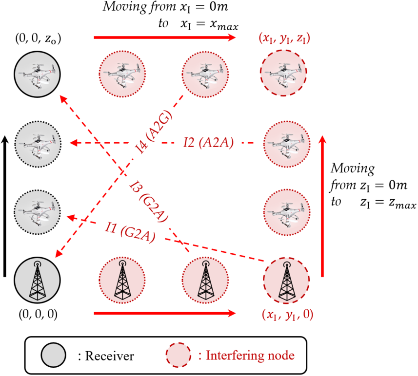
For convenience, we present the simulation scenarios in Fig. 3 and Fig. 4, where $M1-M4$ present the main link between a Tx and a Rx, while $I1-I4$ present the interference link between an interfering node and a Rx. The solid-line arrows mean the case when the node moves in that direction. Unless otherwise specified, the values of simulation parameters presented in Table II are used. Note that the values of $\zeta$ , $\nu$ , and $\mu$ are adopted from [9] for the dense urban environment.

V-A Channel Components

In this subsection, we first compare the LoS probabilities in [8, 37] and the LoS probability of 3GPP (3GPP) model [45], which are the most widely used for UAV communication channels. We then also analyze the LoS probabilities of the G2A and A2A channels.

First, the LoS probabilities in [8, 37, 45] are compared in Figure 5, which shows $p_{\text{L}}(\ell_{\text{m}})$ as a function of the UAV height $d_{\text{m}}^{(\text{V})}$ . The Tx is located at $(x_{\text{m}},y_{\text{m}},0)$ , while the Rx moves from $(0,0,0)$ to $(0,0,z_{\text{m}})$ (i.e., $M1$ case with $d_{\text{m}}^{(\text{H})}=150m$ ). From Fig. 5, we can see that the LoS probability of 3GPP model [45] has some limitaions. Specifically, the LoS probability of 3GPP model is constant regardless of the UAV height, when the UAV height is below 22.5 $m$ , and it increases dramatically at around 22.5 $m$ of the UAV height, which might not be true in reality. On the other hands, the LoS probabilities in [8] and [37] do not have above limitations, but the one in [37] is only valid when the height of the ground device is much smaller than that of the UAV. Hence, we consider the LoS probability model in [37].

Figure 6 presents the LoS probability $p_{\text{L}}(\ell_{\text{m}})$ as a function of the horizontal distance of main link $d_{\text{m}}^{(\text{H})}$ for different values of $z_{\text{o}}$ and $z_{\text{m}}$ . The Rx is located at $(0,0,z_{\text{o}})$ and the Tx moves from $(0,0,z_{\text{m}})$ to $(x_{\text{m}},y_{\text{m}},z_{\text{m}})$ . From this figure, we can see that the LoS probability is a decreasing function as $d_{\text{m}}^{(\text{H})}$ increases because the elevation angle between a Tx and a Rx decreases with $d_{\text{m}}^{(\text{H})}$ . From Fig. 6, we can also see that the LoS probability of the A2A channel is generally higher than the that of the G2A channel since the blockage effect by the obstacle reduces on the A2A channel. However, depending on the height difference between the Tx and the Rx, the LoS probability of the G2A channel (e.g., $z_{\text{m}}=0m$ and $z_{\text{o}}=100m$ ) can be higher than that of the A2A channel (e.g., $z_{\text{m}}=25m$ and $z_{\text{o}}=25m$ ). This is because the elevation angle of the G2A channel is such large, so the probability of forming the LoS link increases.

V-B General Environments vs. Interference-limited Environments

Figure 7 presents the outage probability $p_{\text{o}}(\mathcal{D})$ as a function of the horizontal distance of the interference link $d_{\text{I}}^{(\text{H})}$ , where the Tx and the Rx are located at $(x_{\text{m}},y_{\text{m}},0)$ and $(0,0,z_{\text{o}})$ , respectively (i.e., $M2$ case), while the interfering node moves from $(0,0,0)$ to $(x_{\text{I}},y_{\text{I}},0)$ (i.e., $I3$ case). Here, we use $P_{\text{I}}=P_{\text{m}}$ , $d_{\text{m}}^{(\text{H})}=180m$ , and $d_{\text{m}}^{(\text{V})}=d_{\text{I}}^{(\text{V})}=75m$ . From this figure, we can first see that the analysis results closely match with the simulation results. In addition, the outage probability decreases as $d_{\text{I}}^{(\text{V})}$ increases. This is because as $d_{\text{I}}^{(\text{H})}$ increases, the LoS probability of the interference link decreases while the interference link distance increases with $d_{\text{I}}^{(\text{H})}$ , which results in smaller interference at the Rx. From Fig. 7, we can also see that the outage probability with the general environment (i.e., SINR-based case) has a similar trend to that with the interference-limited environment (i.e., SIR-based case). Hence, in the following figures, we present the numerical results of the interference-limited environments.

V-C Effects of UAV Height

In this subsection, we show the impact of the UAV height on the outage probability according to system parameters.

Figure 8 presents the outage probability $p_{\text{o}}(\mathcal{D})$ as a function of the UAV height $d_{\text{m}}^{(\text{V})}$ . The Tx is located at $(x_{\text{m}},y_{\text{m}},0)$ , while the Rx and the interfering node move from $(0,0,0)$ to $(0,0,z_{\text{o}})$ (i.e., $M1$ case) and move from $(x_{\text{I}},y_{\text{I}},0)$ to $(x_{\text{I}},y_{\text{I}},z_{\text{I}})$ (i.e., $I2$ case), respectively. Here, we use $d_{\text{m}}^{(\text{H})}=80m$ and different values of $\gamma_{\text{t}}$ , $\ell_{\text{I}}$ , and $P_{\text{I}}$ . To focus on the impact of the UAV height on $p_{\text{o}}(\mathcal{D})$ , the environment of the interference link is set to be the same over different height of the UAV, i.e., the interfering node is always located with the fixed distance $\ell_{\text{I}}$ to the Rx and has the A2A channel. From Fig. 8, we can see that the outage probability first increases since the LoS probaility of the interference link rapidly increases at a small height. After the LoS probability of the interference link increases to the end (i.e., $p_{\text{L}}(\ell_{\text{I}})=1$ ), we can see that the outage probability first decreases when the UAV height increases up to a certain value of the UAV height, and then increases. This is because the LoS probability of the main link increases as the UAV height increases. For small UAV height, as the height increases, the increasing probability of forming LoS main link affects more dominantly than the increasing main link distance on the outage probability. However, for large UAV height, the LoS probability does not change that much with the height while the link distance becomes longer, so the outage probability increases. We can also see that the optimal height above a certain UAV height that minimizes $p_{\text{o}}(\mathcal{D})$ decreases as the target SIR $\gamma_{\text{t}}$ or the power of the interfering node $P_{\text{I}}$ increases or the distance of the interference link $\ell_{\text{I}}$ decreases. From this, we can know that the optimal height decreases to reduce the main link distance as the impact of the interference link on the communication improves.

Figure 9 presents the outage probability $p_{\text{o}}(\mathcal{D})$ as a function of the UAV height $d_{\text{o}}^{(\text{V})}$ . The Tx is located at $(x_{\text{m}},y_{\text{m}},0)$ (i.e., $M1$ case) and the interfering node is located at $(x_{\text{I}},y_{\text{I}},0)$ (i.e., $I1$ case), while the Rx moves from $(0,0,0)$ to $(0,0,z_{\text{o}})$ . Here, we use $d_{\text{m}}^{(\text{H})}=80m$ and different values of $\gamma_{\text{t}}$ , $d_{\text{I}}^{(\text{H})}$ , and $P_{\text{I}}$ . To focus on the impact of the UAV height on $p_{\text{o}}(\mathcal{D})$ , we vary the height of the Rx, i.e., $d_{\text{o}}^{(\text{V})}$ , where $d_{\text{m}}^{(\text{V})}=d_{\text{I}}^{(\text{V})}=d_{\text{o}}^{(\text{V})}$ , and the Tx and the interfering node are located on the ground. In this case, the LoS probability of the main link is higher than that of the interference link due to $d_{\text{m}}^{(\text{H})}<d_{\text{I}}^{(\text{H})}$ . From Fig. 9, we can see that the outage probability first decreases as the height increases up to a certain value of the UAV height, and then increases. This is because not only the LoS probability of the main link but also that of the interference link increase with the UAV height. However, for large UAV height, the LoS probability of the interference link increases more than that of the main link. We can also see that the optimal height increases as $\gamma_{\text{t}}$ or $P_{\text{I}}$ increases or $\ell_{\text{I}}$ decreases to improve the LoS probability of the main link unlike the case in Fig. 8.

V-D Effects of Main and Interference Link Environments

In this subsection, we focus on the impact of the environment of the main and interference links on the outage probability.

Figure 10 presents the outage probability $p_{\text{o}}(\mathcal{D})$ as a function of the horizontal distance of the interference link $d_{\text{I}}^{(\text{H})}$ with $P_{\text{I}}=P_{\text{m}}$ for different values of $d_{\text{I}}^{(\text{V})}$ and channel environment of the main link. In Fig. 10, two scenarios are considered: A2A main link with G2A interference link (A2A-G2A) and G2G main link with A2G interference link (G2G-A2G). The A2A-G2A case maps to $M3$ with $I3$ , and the G2G-A2G case maps to $M4$ with $I4$ in Fig. 3 and Fig. 4. Note that to explore the impact of the horizontal and vertical distances of interference link in this figure, the horizontal distance of interference link $d_{\text{I}}^{(\text{H})}$ is varied when the vertical distance $d_{\text{I}}^{(\text{V})}=50m$ or $100m$ . To focus on the impact of the horizontal and vertical distance of the interference link, the main link is set as the A2A or the G2G channel with a fixed link distance 100 $m$ . The interference link is the A2G or the G2A channel. From this figure, we can see that generally, longer horizontal distance of the interference link (i.e., larger $d_{\text{I}}^{(\text{H})}$ ) results in lower outage probability. On the other hand, longer vertical distance of the interference link (i.e., larger $d_{\text{I}}^{(\text{V})}$ ) does not always result in upper outage probability. Specifically, when the main link is the A2A channel, the outage probability is smaller with $d_{\text{I}}^{(\text{V})}=100m$ than that with $d_{\text{I}}^{(\text{V})}=50m$ . This is because, the LoS probability of the main link with $d_{\text{m}}^{(\text{V})}=50m$ is smaller than that with $d_{\text{m}}^{(\text{V})}=100m$ even though the LoS probability of the interference link with $d_{\text{I}}^{(\text{V})}=50m$ decreases faster than that with $d_{\text{I}}^{(\text{V})}=100m$ as $d_{\text{I}}^{(\text{H})}$ increases.

Figure 11 presents the outage probabilities for LoS main and interference links $p_{\text{o}}^{(\text{L,L})}(\mathcal{D})$ and NLoS main and interference links $p_{\text{o}}^{(\text{N,N})}(\mathcal{D})$ as a function of $\frac{\beta_{\text{m}}(\ell_{\text{m}})}{\beta_{\text{I}}(\ell_{\text{I}})}$ for different values of $\gamma_{\text{t}}$ . This is the case of $I3$ (G2A) with $M2$ (G2A) in Fig. 3 and Fig. 4, and we use $d_{\text{m}}^{(\text{H})}=100m$ and $d_{\text{I}}^{(\text{V})}=d_{\text{m}}^{(\text{V})}=70m$ . From this figure, we can confirm that both outage probabilities are monotonic decreasing functions with $\frac{\beta_{\text{m}}(\ell_{\text{m}})}{\beta_{\text{I}}(\ell_{\text{I}})}$ . In addition, there exists a cross point of those probabilities at around $\frac{\beta_{\text{m}}(\ell_{\text{m}})}{\beta_{\text{I}}(\ell_{\text{I}})}=1.55$ when the target SIR $\gamma_{\text{t}}=2$ . For smaller $\frac{\beta_{\text{m}}(\ell_{\text{m}})}{\beta_{\text{I}}(\ell_{\text{I}})}<1.55$ , $p_{\text{o}}^{(\text{L,L})}(\mathcal{D})$ is greater than $p_{\text{o}}^{(\text{N,N})}(\mathcal{D})$ , but it becomes opposite for larger $\frac{\beta_{\text{m}}(\ell_{\text{m}})}{\beta_{\text{I}}(\ell_{\text{I}})}>1.55$ . This verifies the results in Corollary 1 that the NLoS environment can be more preferred for small $\frac{\beta_{\text{m}}(\ell_{\text{m}})}{\beta_{\text{I}}(\ell_{\text{I}})}$ . We can also see that the value of the cross point increases from $1.55$ to $2.35$ as the target SIR $\gamma_{\text{t}}$ increases from $2$ to $4$ . Hence, we can know that the range of $\frac{\beta_{\text{m}}(\ell_{\text{m}})}{\beta_{\text{I}}(\ell_{\text{I}})}$ where the NLoS environment is preferred increases as the target SIR $\gamma_{\text{t}}$ increases.

V-E Effects of Multiple Interfering Nodes

In this subsection, we present how the outage probability is changed when we consider multiple interfering nodes, compared to the case of considering one dominant interfering node. Here, we define the dominant interfering node as the nearest one to the Rx, which gives the largest interference to the Rx on average.

When we consider one nearest interfering node among multiple interfering nodes, which are distributed in PPP $\Phi_{\text{I}}$ , the outage probability $p_{\text{o,n}}(\ell_{\text{m}})$ can also be obtained using the outage probability for single interfering node case $\hat{p}_{\text{o}}^{({e_{\text{m}},e_{\text{I}}})}(\mathcal{D})$ in (15) as

	$\displaystyle p_{\text{o,n}}(\ell_{\text{m}})$	$\displaystyle=\int_{0}^{\infty}\sum_{e_{\text{m}},e_{\text{I}}\in\{\text{L},\text{N}\}}\hat{p}_{\text{o}}^{(e_{\text{m}},e_{\text{I}})}\left(\sqrt{r^{2}+z_{\text{o}}^{2}}\right)$
		$\displaystyle\quad\times p_{e_{\text{m}}}(\ell_{\text{m}})p_{e_{\text{I}}}(r)f_{d_{\text{I}}^{(\text{H})}}(r)\,dr$		(33)

where $\hat{p}_{\text{o}}^{(e_{\text{m}},e_{\text{I}})}\left(\sqrt{r^{2}+z_{\text{o}}^{2}}\right)$ is the outage probability for an arbitrary interfering node and $f_{d_{\text{I}}^{(\text{H})}}(r)=2\lambda_{\text{I}}\pi r\exp(-\lambda_{\text{I}}\pi r^{2})$ is the PDF of the horizontal distance to the nearest interfering node from the Rx.

Figure 12 presents the outage probability with multiple interfering nodes, $p_{\text{o,m}}(\ell_{\text{m}})$ in Corollary 2, and that with one nearest interfering node, $p_{\text{o,n}}(\ell_{\text{m}})$ in (V-E) as a function of the UAV height $d_{\text{o}}^{(\text{V})}$ for different values of the interfering node density $\lambda_{\text{I}}$ and the target SIR $\gamma_{\text{t}}$ . For this figure, the Tx is located at $(80m,0,0)$ , and the location of Rx is changed from $(0,0,0)$ to $(0,0,250m)$ (i.e., $M1$ case). The multiple interfering nodes are located on the ground (i.e., $I1$ case). Here, we also use $R=5000m$ , $d_{\text{m}}^{(\text{H})}=80m$ , and $P_{\text{I}}=P_{\text{m}}$ . In addition, since the multiple interfering nodes are randomly distributed in PPP, $d_{\text{I}}^{(\text{H})}$ becomes random, of which PDF depends on the interfering node density $\lambda_{\text{I}}$ . As Fig. 9, the outage probability first decreases as the height increases up to a certain value of the UAV height, and then increases.

From this figure, we can see that the outage probability for the case of considering one dominant interfering node has the similar trend with that for the multiple interfering nodes case. The difference in the outage probability for those two cases increase as the interfering node density $\lambda_{\text{I}}$ increases. This is because, as $\lambda_{\text{I}}$ increases, although the dominant interfering node can be located closer to Rx and generate larger interference, the amount of the interference from multiple interfering nodes increases more in the multiple interfering node case, which makes larger difference in the outage probabilities.

However, when the UAV height is the optimal (like around 70m in Fig. 12) in terms of minimizing the outage probability, the outage probabilities of those two cases become almost the same. Therefore, from this result, we can see that the analysis result for the case of considering one interfering node, presented in this work, can also be usefully used for the optimal design of UAV networks with multiple interfering nodes such as the optimal UAV height determination.

Figure 13 presents the outage probability with multiple interfering nodes, $p_{\text{o,m}}(\ell_{\text{m}})$ in Corollary 2, and that with one nearest interfering node, $p_{\text{o,n}}(\ell_{\text{m}})$ in (V-E) as a function of the UAV height $d_{\text{m}}^{(\text{V})}$ for different values of the interfering node density $\lambda_{\text{I}}$ . For this figure, the Tx is located at $(80m,0,0)$ , and the location of Rx is changed from $(0,0,0)$ to $(0,0,500m)$ (i.e., $M1$ case). The multiple interfering nodes are located in the air (i.e., $I2$ case), and we use $R=5000m$ , $d_{\text{m}}^{(\text{H})}=80m$ , and $P_{\text{I}}=0.3P_{\text{m}}$ .

From this figure, we can see that the outage probability of one dominant interfering node has the similar trend with that of the multiple interfering nodes case. However, since most of interfering nodes are in LoS environment, the optimal UAV heights that minimizes the outage probability of those two cases have a difference. Nevertheless, the optimal height of one dominant interfering node case can be used for the upper bound of that of the multiple interfering nodes case. Hence, we can see that the analysis result for the case of considering one interfering node, presented in this work, can also be used to give insights for the optimal design of UAV networks with multiple interfering nodes even if the multiple interfering nodes are in the A2A channel.

Figure 14 shows the network outage probability as a function of UAV height when $R=5000m$ and $P_{\text{I}}=P_{\text{m}}$ for different values of the transmitting node density $\lambda_{\text{I}}$ . From this figure, we can see that as $\lambda_{\text{I}}$ increases, the optimal UAV height decreases, while the optimal outage probability increases. Lowering the optimal UAV height can increase both the received interference power from other transmitting nodes and the main link received power. Hence, from the results of this figure, we can see that when $\lambda_{\text{I}}$ is larger, the optimal UAV height becomes smaller as increasing the received power of the main link becomes more dominantly determined the outage probability than the increasing interference power.

VI Conclusion

This paper analyzes the impact of the interfering node for reliable UAV communications. After characterizing the channel model affected by the horizontal distance and the vertical distance of the communication link, we derive the outage probability in a closed-form for all possible scenarios of main and interference links. Furthermore, we show the effects of the transmission power, the horizontal link and vertical link distances, and the communication scenarios of main and interference links. Specifically, we show the existence of the optimal heights of the UAV for various scenarios, which increase as the power of the interfering node decreases or the interference link distance increases. We also analytically prove that the NLoS environment can be better than the LoS environment if the average received power of the interference is much larger than that of the main link signal. The outcomes of this work can be usefully used for the optimal height determination of UAV in the presence of an interfering node, and it can give insights on the UAV height for the multiple interfering nodes case as well.

-A Proof of Theorem 1

As the main and interference links can be in either the LoS or NLoS environments when the probability is $p_{\text{L}}(\ell_{i})$ or $p_{\text{N}}(\ell_{i})$ , respectively, the outage probability is divided into four cases, which are $p_{\text{o}}\!^{(\text{L,L})}(\mathcal{D})$ , $p_{\text{o}}\!^{(\text{L,N})}(\mathcal{D})$ , $p_{\text{o}}\!^{(\text{N,L})}(\mathcal{D})$ , and $p_{\text{o}}\!^{(\text{N,N})}(\mathcal{D})$ according to the environments of main and interference links. Hence, the outage probability is obtained as (1) using the law of total probability. We derive $p_{\text{o}}^{({e_{\text{m}},e_{\text{I}}})}(\mathcal{D})$ for the above four cases as follows.

For Case 1, $K_{\text{m}}(\ell_{\text{m}})\neq 0$ and $K_{\text{I}}(\ell_{\text{I}})\neq 0$ as both main and interference links are in LoS environments, and $p_{\text{o}}\!^{(\text{L,L})}(\mathcal{D})$ can be obtained using (7) as

\displaystyle p_{\text{o}}\!^{(\text{L,L})}(\mathcal{D})=\int_{0}^{\infty}\hskip-5.69054pt\int_{0}^{\frac{\gamma_{\text{t}}(\beta_{\text{I}}(\ell_{\text{I}})g+N_{\text{o}})}{\beta_{\text{m}}(\ell_{\text{m}})}}f_{h_{\text{m}}}(h)\,dhf_{h_{\text{I}}}(g)\,dg.

(34)

By using the CDF (CDF) of the noncentral Chi-squared distribution in (34), $p_{\text{o}}\!^{(\text{L,L})}(\mathcal{D})$ is presented as (11).

In Case 2, $K_{\text{m}}(\ell_{\text{m}})\neq 0$ and $K_{\text{I}}(\ell_{\text{I}})=0$ as the interference link is in the NLoS environment, and $p_{\text{o}}\!^{(\text{L,N})}(\mathcal{D})$ is obtained using (7) and (8) as

		$\displaystyle p_{\text{o}}\!^{(\text{L,N})}(\mathcal{D})=\int_{0}^{\infty}\int_{0}^{\frac{\gamma_{\text{t}}(\beta_{\text{I}}(\ell_{\text{I}})g+N_{\text{o}})}{\beta_{\text{m}}(\ell_{\text{m}})}}f_{h_{\text{m}}}(h)\,dhf_{h_{\text{I}}}(g)\,dg$
		$\displaystyle\overset{\underset{\mathrm{(a)}}{}}{=}1-\hskip-2.84526pt\int_{0}^{\infty}\hskip-2.84526ptQ\hskip-1.42262pt\left(\hskip-2.84526pt\sqrt{2K_{\text{m}}(\ell_{m})},\sqrt{\frac{\gamma_{\text{t}}(\beta_{\text{I}}(\ell_{\text{I}})g\hskip-1.42262pt+\hskip-2.84526ptN_{\text{o}})}{\beta_{\text{m}}(\ell_{\text{m}})}}\right)\hskip-1.42262pt\exp\hskip-1.42262pt\left(-g\right)\,\hskip-2.84526ptdg$
		$\displaystyle\overset{\underset{\mathrm{(b)}}{}}{=}1-\frac{\beta_{\text{m}}(\ell_{\text{m}})}{\gamma_{\text{t}}\beta_{\text{I}}(\ell_{\text{I}})}\exp\left(\frac{N_{\text{o}}}{\beta_{\text{I}}(\ell_{\text{I}})}\right)$
		$\displaystyle\quad\times\hskip-2.84526pt\int_{\frac{\gamma_{\text{t}}N_{\text{o}}}{\beta_{\text{m}}(\ell_{\text{m}})}}^{\infty}\hskip-2.84526ptQ\hskip-1.42262pt\left(\hskip-1.42262pt\sqrt{2K_{\text{m}}(\ell_{\text{m}})},\sqrt{g^{\prime}}\right)\exp\hskip-1.42262pt\left(\hskip-1.42262pt-\frac{\beta_{\text{m}}(\ell_{\text{m}})g^{\prime}}{\gamma_{\text{t}}\beta_{\text{I}}(\ell_{\text{I}})}\right)\,\hskip-2.84526ptdg^{\prime}\hskip-5.69054pt$		(35)

where $Q(a,b)$ is the first-order Marcum Q-function. In (35), (a) is from the CDF of the noncentral Chi-squared distribution, (b) is obtained by substitution from $\frac{\gamma_{\text{t}}\beta_{\text{I}}(\ell_{\text{I}})}{\beta_{\text{m}}(\ell_{\text{m}})}g+\frac{\gamma_{\text{t}}N_{\text{o}}}{\beta_{\text{m}}(\ell_{\text{m}})}$ to $g^{\prime}$ , and the integral term can be represented as

		$\displaystyle\int_{\frac{d^{2}}{2}}^{\infty}\exp\left(-c^{2}x\right)Q\left(e,f\sqrt{2x}\right)\,dx$
		$\displaystyle=\frac{1}{c^{2}}\left\{\exp\left(-\frac{c^{2}d^{2}}{2}\right)Q(e,df)-\frac{c^{2}}{c^{2}+f^{2}}\right.$
		$\displaystyle\quad\left.\times\exp\hskip-1.42262pt\left(\hskip-1.42262pt-\frac{c^{2}e^{2}}{2(c^{2}+f^{2})}\hskip-1.42262pt\right)\hskip-1.42262ptQ\hskip-1.42262pt\left(\hskip-1.42262pt\frac{ef}{\sqrt{c^{2}+f^{2}}},d\sqrt{c^{2}+f^{2}}\right)\hskip-2.84526pt\right\}\hskip-2.84526pt$		(36)

where $c=\sqrt{\frac{\beta_{\text{m}}(\ell_{\text{m}})}{\gamma_{\text{t}}\beta_{\text{I}}(\ell_{\text{I}})}}$ , $d=\sqrt{\frac{2\gamma_{\text{t}}N_{\text{o}}}{\beta_{\text{m}}(\ell_{\text{m}})}}$ , $e=\sqrt{2K_{\text{m}}(\ell_{\text{m}})}$ , and $f=\sqrt{\frac{1}{2}}$ from [46, eq. (40)]. By using (-A) in (35), $p_{\text{o}}\!^{(\text{L,N})}(\mathcal{D})$ is presented as (12).

In Case 3, $K_{\text{m}}(\ell_{\text{m}})=0$ and $K_{\text{I}}(\ell_{\text{I}})\neq 0$ as the main link is in the NLoS environment, and $p_{\text{o}}\!^{(\text{N,L})}(\mathcal{D})$ is given by

		$\displaystyle p_{\text{o}}\!^{(\text{N,L})}(\mathcal{D})=\int_{0}^{\infty}\int_{0}^{\frac{\gamma_{\text{t}}(\beta_{\text{I}}(\ell_{\text{I}})g+N_{\text{o}})}{\beta_{\text{m}}(\ell_{\text{m}})}}f_{h_{\text{m}}}(h)\,dhf_{h_{\text{I}}}(g)\,dg$
		$\displaystyle\overset{\underset{\mathrm{(a)}}{}}{=}1-\frac{1}{2}\int_{0}^{\infty}\exp\left(-\frac{\gamma_{\text{t}}(\beta_{\text{I}}(\ell_{\text{I}})g+N_{\text{o}})}{\beta_{\text{m}}(\ell_{\text{m}})}\right)$
		$\displaystyle\quad\times\exp\left(-K_{\text{I}}(\ell_{\text{I}})-\frac{g}{2}\right)I_{0}\left(\sqrt{2K_{\text{I}}(\ell_{\text{I}})g}\right)\,dg.$		(37)

In (-A), (a) is from the CDF of the exponential distribution and the integral term can be presented as

\displaystyle\int_{0}^{\infty}\exp(-c^{2}x)I_{0}\left(d\sqrt{2x}\right)\,dx=\frac{1}{c^{2}}\exp\left(\frac{d^{2}}{2c^{2}}\right)

(38)

where $c=\sqrt{\frac{1}{2}+\frac{\gamma_{\text{t}}\beta_{\text{I}}(\ell_{\text{I}})}{\beta_{\text{m}}(\ell_{\text{m}})}}$ and $d=\sqrt{K_{\text{I}}(\ell_{\text{I}})}$ from [46, eq. (9)]. By using (38) in (-A), $p_{\text{o}}\!^{(\text{N,L})}(\mathcal{D})$ is presented as (13).

In Case 4, $K_{\text{m}}(\ell_{\text{m}})=0$ and $K_{\text{I}}(\ell_{\text{I}})=0$ as the main and the interference links are both in NLoS environments, and $p_{\text{o}}\!^{(\text{N,N})}(\mathcal{D})$ is given by

		$\displaystyle p_{\text{o}}\!^{(\text{N,N})}(\mathcal{D})=\int_{0}^{\infty}\int_{0}^{\frac{\gamma_{\text{t}}(\beta_{\text{I}}(\ell_{\text{I}})g+N_{\text{o}})}{\beta_{\text{m}}(\ell_{\text{m}})}}f_{h_{\text{m}}}(h)\,dhf_{h_{\text{I}}}(g)\,dg$
		$\displaystyle\overset{\underset{\mathrm{(a)}}{}}{=}1-\int_{0}^{\infty}\exp\left(-\frac{\gamma_{\text{t}}(\beta_{\text{I}}(\ell_{\text{I}})g+N_{\text{o}})}{\beta_{\text{m}}(\ell_{\text{m}})}-g\right)\,dg$		(39)

where (a) is from the CDF of the exponential distribution. By simple calculation, $p_{\text{o}}\!^{(\text{N,N})}(\mathcal{D})$ is presented as (14).

-B Proof of Lemma 1

In the interference-limited environment, the interfering signal power is much stronger than the noise power (i.e., $h_{\text{I}}\beta_{\text{I}}(\ell_{\text{I}})\gg N_{\text{o}}$ ), so the noise is negligible. Consequently, the communication performance can be analyzed based on $\hat{\gamma}(\ell_{\text{m}},\ell_{\text{I}})=\frac{h_{\text{m}}\beta_{\text{m}}(\ell_{\text{m}})}{h_{\text{I}}\beta_{\text{I}}(\ell_{\text{I}})}$ instead of $\gamma(\ell_{\text{m}},\ell_{\text{I}})=\frac{h_{\text{m}}\beta_{\text{m}}(\ell_{\text{m}})}{h_{\text{I}}\beta_{\text{I}}(\ell_{\text{I}})+N_{\text{o}}}$ . Hence, the integral interval in the outage probability substitutes from $\left[0,\frac{\gamma_{\text{t}}(h_{\text{I}}\beta_{\text{I}}(\ell_{\text{I}})+N_{\text{o}})}{\beta_{\text{m}}(\ell_{\text{m}})}\right]$ to $\left[0,\frac{\gamma_{\text{t}}h_{\text{I}}\beta_{\text{I}}(\ell_{\text{I}})}{\beta_{\text{m}}(\ell_{\text{m}})}\right]$ , and we obtain $\hat{p}_{\text{o}}^{({e_{\text{m}},e_{\text{I}}})}(\mathcal{D})$ for the above four cases as follows.

For Case 1, i.e., $K_{\text{m}}(\ell_{\text{m}})\neq 0$ and $K_{\text{I}}(\ell_{\text{I}})\neq 0$ , we can present $\hat{p}_{\text{o}}\!^{(\text{L,L})}(\mathcal{D})$ by replacing $N_{\text{o}}=0$ in (11) as

$\displaystyle\hat{p}_{\text{o}}\!^{(\text{L,L})}(\mathcal{D})$	$\displaystyle=\int_{0}^{\infty}\hskip-5.69054pt\int_{0}^{\frac{\gamma_{\text{t}}\beta_{\text{I}}(\ell_{\text{I}})g}{\beta_{\text{m}}(\ell_{\text{m}})}}f_{h_{\text{m}}}(h)\,dhf_{h_{\text{I}}}(g)\,dg$
	$\displaystyle\overset{\underset{\mathrm{(a)}}{}}{=}1-\frac{1}{2}\int_{0}^{\infty}Q\left(\sqrt{2K_{\text{m}}(\ell_{\text{m}})},\sqrt{\frac{\gamma_{\text{t}}\beta_{\text{I}}(\ell_{\text{I}})g}{\beta_{\text{m}}(\ell_{\text{m}})}}\right)$
	$\displaystyle\quad\times\exp\left(-K_{\text{I}}(\ell_{\text{I}})-\frac{g}{2}\right)I_{0}\left(\sqrt{2K_{\text{I}}(\ell_{\text{I}})g}\right)\,dg$	(40)

where (a) is from the CDF of the noncentral Chi-squared distribution and the integral term in (40) can be presented as

		$\displaystyle\int_{0}^{\infty}\exp\left(-c^{2}x\right)I_{0}\left(d\sqrt{2x}\right)Q\left(e,f\sqrt{2x}\right)\,dx$
		$\displaystyle=\frac{1}{c^{2}}\left\{\exp\left(\frac{d^{2}}{2c^{2}}\right)Q\left(\frac{ce}{\sqrt{{c}^{2}+{f}^{2}}},\frac{df}{c\sqrt{{c}^{2}+{f}^{2}}}\right)\right.$
		$\displaystyle\quad\left.-\frac{f^{2}}{c^{2}+f^{2}}\exp\left(\frac{d^{2}-c^{2}e^{2}}{2(c^{2}+f^{2})}\right)I_{0}\left(\frac{def}{c^{2}+f^{2}}\right)\right\}$		(41)

where $c=\sqrt{0.5}$ , $d=\sqrt{K_{\text{I}}(\ell_{\text{I}})}$ , $e=\sqrt{2K_{\text{m}}(\ell_{\text{m}})}$ , and $f=\sqrt{\frac{\gamma_{\text{t}}\beta_{\text{I}}(\ell_{\text{I}})}{2\beta_{\text{m}}(\ell_{\text{m}})}}$ from [46, eq. (46)]. By using (-B) in (40), $\hat{p}_{\text{o}}\!^{(\text{L,L})}(\mathcal{D})$ is presented as (17).

In Case 2, i.e., $K_{\text{m}}(\ell_{\text{m}})\neq 0$ and $K_{\text{I}}(\ell_{\text{I}})=0$ , $\hat{p}_{\text{o}}\!^{(\text{L,N})}(\mathcal{D})$ is presented using (35) as

$\displaystyle\hat{p}_{\text{o}}\!^{(\text{L,N})}(\mathcal{D})$	$\displaystyle=\int_{0}^{\infty}\hskip-5.69054pt\int_{0}^{\frac{\gamma_{\text{t}}\beta_{\text{I}}(\ell_{\text{I}})g}{\beta_{\text{m}}(\ell_{\text{m}})}}f_{h_{\text{m}}}(h)\,dhf_{h_{\text{I}}}(g)\,dg$
	$\displaystyle\overset{\underset{\mathrm{(a)}}{}}{=}1-\int_{0}^{\infty}Q\left(\sqrt{2K_{\text{m}}(\ell_{\text{m}})},\sqrt{\frac{\gamma_{\text{t}}\beta_{\text{I}}(\ell_{\text{I}})g}{\beta_{\text{m}}(\ell_{\text{m}})}}\right)$
	$\displaystyle\quad\times\exp\left(-g\right)\,dg$	(42)

where (a) is from the CDF of the noncentral Chi-squared distribution and the integral term in (-B) can be presented as (-A) with $c=1$ , $d=0$ $e=\sqrt{2K_{\text{m}}(\ell_{\text{m}})}$ , and $f=\sqrt{\frac{\gamma_{\text{t}}\beta_{\text{I}}(\ell_{\text{I}})}{2\beta_{\text{m}}(\ell_{\text{m}})}}$ . By using (-A) in (-B), $\hat{p}_{\text{o}}\!^{(\text{L,N})}(\mathcal{D})$ is presented as (18).

In Case 3, i.e., $K_{\text{m}}(\ell_{\text{m}})=0$ and $K_{\text{I}}(\ell_{\text{I}})\neq 0$ , $\hat{p}_{\text{o}}\!^{(\text{N,L})}(\mathcal{D})$ is obtained by making $N_{\text{o}}=0$ in (13) as (19). In Case 4, i.e., $K_{\text{m}}(\ell_{\text{m}})=0$ and $K_{\text{I}}(\ell_{\text{I}})=0$ , $\hat{p}_{\text{o}}\!^{(\text{N,N})}(\mathcal{D})$ is obtained by making $N_{\text{o}}=0$ in (14) as (20).

-C Proof of Corollary 2

For the multiple interfering nodes case, the outage probability can be presented as

\displaystyle p_{\text{o,m}}(\ell_{\text{m}})

\displaystyle=p_{\text{o,m}}^{(\text{L})}(\ell_{\text{m}})p_{\text{L}}(\ell_{\text{m}})\hskip-1.42262pt+\hskip-1.42262ptp_{\text{o,m}}^{(\text{N})}(\ell_{\text{m}})p_{\text{N}}(\ell_{\text{m}})\hskip-2.84526pt

(43)

where $p_{\text{o,m}}^{(\text{L})}(\ell_{\text{m}})$ and $p_{\text{o,m}}^{(\text{N})}(\ell_{\text{m}})$ are the outage probabilities for LoS and NLoS main links, respectively. When we consider the Nakagami-m fading for the LoS link and the interference-limited environment to derive the outage probability tractably, $p_{\text{o,m}}^{(\text{L})}(\ell_{\text{m}})$ is given by

		$\displaystyle p_{\text{o,m}}^{(\text{L})}(\ell_{\text{m}})=\mathbb{E}\left[\mathbb{P}\left[h_{\text{m}}<\frac{\gamma_{\text{t}}I}{\beta_{\text{m}}(\ell_{\text{m}})}\bigg\|I\right]\right]$
		$\displaystyle\overset{\underset{\mathrm{(a)}}{}}{=}1-\mathbb{E}\left[\frac{\Gamma\left(m,\frac{m\gamma_{\text{t}}I}{\beta_{\text{m}}(\ell_{\text{m}})}\right)}{\Gamma(m)}\right]$
		$\displaystyle\overset{\underset{\mathrm{(b)}}{}}{=}1-\mathbb{E}\left[\sum_{k=0}^{m-1}\frac{1}{k!}\left(\frac{m\gamma_{\text{t}}I}{\beta_{\text{m}}(\ell_{\text{m}})}\right)^{k}\exp\left(-\frac{m\gamma_{\text{t}}I}{\beta_{\text{m}}(\ell_{\text{m}})}\right)\right]$
		$\displaystyle=1-\sum_{k=0}^{m-1}\frac{1}{k!}\left(-\frac{m\gamma_{\text{t}}}{\beta_{\text{m}}(\ell_{\text{m}})}\right)^{k}\left[\frac{\partial}{\partial s^{k}}\mathcal{L}_{I}(s)\right]_{s=\frac{m\gamma_{\text{t}}}{\beta_{\text{m}}(\ell_{\text{m}})}}$		(44)

where $I=\sum_{u\in\Phi_{\text{I}}\backslash\{u_{\text{o}}\}}h_{u}\ell_{u}^{-\alpha_{u}(\ell_{u})}P_{\text{I}}$ is the interference from multiple interfering nodes, (a) is obtained because $h_{m}\sim\Gamma(m,1/m)$ , and (b) follows from the definition of incomplete gamma function for integer values of $m$ .³³ 3 Note that (a) can be obtained only when $m=\frac{K_{\text{m}}(\ell_{\text{m}})^{2}+2K_{\text{m}}(\ell_{\text{m}})+1}{2K_{\text{m}}(\ell_{\text{m}})+1}$ is an integer. Hence, we cannot obtain $p_{\text{o,m}}^{(\text{L})}(\ell_{\text{m}})$ for all scenarios. In (-C), $\mathcal{L}_{I}(s)$ is the Laplace transform of the interference $I$ , and is given by

$\displaystyle\mathcal{L}_{I}(s)$	$\displaystyle=\mathbb{E}_{\Phi_{\text{I}}\backslash\{u_{\text{o}}\}}\hskip-2.84526pt\left[\exp\left(-s\sum_{u\in\Phi_{\text{I}}\backslash\{u_{\text{o}}\}}P_{\text{I}}h_{u}\ell_{u}^{-\alpha_{u}(\ell_{u})}\right)\right]$
	$\displaystyle=\mathbb{E}_{\Phi_{\text{I}}\backslash\{u_{\text{o}}\}}\hskip-2.84526pt\left[\prod_{u\in\Phi_{\text{I}}\backslash\{u_{\text{o}}\}}\mathbb{E}_{h_{u}}\hskip-1.42262pt\left[\exp\left(-sh_{u}\ell_{u}^{-\alpha_{u}(\ell_{u})}P_{\text{I}}\right)\right]\right]$
	$\displaystyle\overset{\underset{\mathrm{(a)}}{}}{=}\exp\left\{-2\pi\lambda_{\text{I}}\int_{r}^{\infty}\sum_{e_{\text{I}}\in\{\text{L},\text{N}\}}\left(1\hskip-1.42262pt-\hskip-1.42262pt\hat{p}_{\text{o}}^{(\text{L},e_{\text{I}})}\hskip-2.84526pt\left(\sqrt{t^{2}+z_{\text{o}}^{2}}\right)\hskip-1.42262pt\right)\right.$
	$\displaystyle\quad\times\hskip-2.84526pt\left.p_{e_{\text{I}}}(t)t\,dt\right\}$	(45)

where (a) is from the PGFL (PGFL) [42]. In (43), $p_{\text{o,m}}^{(\text{N})}(\ell_{\text{m}})$ is given by

		$\displaystyle p_{\text{o,m}}^{(\text{N})}(\ell_{\text{m}})=\mathbb{E}\left[\mathbb{P}\left[h_{\text{m}}<\frac{\gamma_{\text{t}}I}{\beta_{\text{m}}(\ell_{\text{m}})}\bigg\|I\right]\right]$
		$\displaystyle\overset{\underset{\mathrm{(a)}}{}}{=}1-\mathbb{E}\left[\exp\left(-\frac{\gamma_{\text{t}}I}{\beta_{\text{m}}(\ell_{\text{m}})}\right)\right]$
		$\displaystyle=1-\mathbb{E}_{\Phi_{\text{I}}\backslash\{u_{\text{o}}\}}\hskip-1.42262pt\left[\prod_{u\in\Phi_{\text{I}}\backslash\{u_{\text{o}}\}}\hskip-1.42262pt\mathbb{E}_{h_{u}}\hskip-1.42262pt\left[\exp\hskip-1.42262pt\left(-\frac{\gamma_{\text{t}}h_{u}\ell_{u}^{-\alpha_{u}(\ell_{u})}P_{\text{I}}}{\beta_{\text{m}}(\ell_{\text{m}})}\right)\right]\right]$
		$\displaystyle\overset{\underset{\mathrm{(b)}}{}}{=}1-\exp\left\{-2\pi\lambda_{\text{I}}\int_{r}^{\infty}\sum_{e_{\text{I}}\in\{\text{L},\text{N}\}}\left(1-\hat{p}_{\text{o}}^{(\text{N},e_{\text{I}})}\left(\sqrt{t^{2}+z_{\text{o}}^{2}}\right)\right)\right.$
		$\displaystyle\quad\times\left.p_{e_{\text{I}}}(t)t\,dt\right\}$		(46)

where (a) is obtained because $h_{\text{m}}\sim\exp(1)$ and (b) is from the PGFL.

References

[1] M. Kim and J. Lee, “Outage probability of UAV communications in the presence of interference,” in Proc. IEEE Global Commun. Conf. (GLOBECOM), Abu Dhabi, UAE, Dec. 2018, pp. 1–6.
[2] L. Gupta, R. Jain, and G. Vaszkun, “Survey of important issues in UAV communication networks,” IEEE Commun. Surveys Tuts., vol. 18, no. 2, pp. 1123–1152, Second Quart. 2016.
[3] Y. Zeng, R. Zhang, and T. J. Lim, “Wireless communications with unmanned aerial vehicles: opportunities and challenges,” IEEE Commun. Mag., vol. 54, no. 5, pp. 36–42, May 2016.
[4] S. Hayat, E. Yanmaz, and R. Muzaffar, “Survey on unmanned aerial vehicle networks for civil applications: a communications viewpoint,” IEEE Commun. Surveys Tuts., vol. 18, no. 4, pp. 2624–2661, Fourth Quart. 2016.
[5] W. Khawaja, I. Guvenc, D. Matolak, U. C. Fiebig, and N. Schneckenberger, “A survey of air-to-ground propagation channel modeling for unmanned aerial vehicles,” IEEE Commun. Surveys Tuts., vol. 21, no. 3, pp. 2361–2391, Third Quart. 2019.
[6] Q. Zhang, H. H. Yang, T. Q. S. Quek, and J. Lee, “Heterogeneous cellular networks with LoS and NLoS transmissions-the role of Massive MIMO and small cells,” IEEE Trans. Wireless Commun., vol. 16, no. 12, pp. 7996–8010, Dec. 2017.
[7] H. Cho, C. Liu, J. Lee, T. Noh, and T. Q. S. Quek, “Impact of elevated base stations on the ultra-dense networks,” IEEE Commun. Lett., vol. 22, no. 6, pp. 1268–1271, Jun. 2018.
[8] A. Al-Hourani, S. Kandeepan, and S. Lardner, “Optimal LAP altitude for maximum coverage,” IEEE Wireless Commun. Lett., vol. 3, no. 6, pp. 569–572, Dec. 2014.
[9] R. I. B. Yaliniz, A. El-Keyi, and H. Yanikomeroglu, “Efficient 3-D placement of an aerial base station in next generation cellular networks,” in Proc. IEEE Int. Conf. Commun. (ICC), Kuala Lumpur, Malaysia, May 2016, pp. 1–5.
[10] M. Alzenad, A. El-Keyi, F. Lagum, and H. Yanikomeroglu, “3-D placement of an unmanned aerial vehicle base station (UAV-BS) for energy-efficient maximal coverage,” IEEE Commun. Lett., vol. 6, no. 4, pp. 434–437, Aug. 2017.
[11] Y. Chen, W. Feng, and G. Zheng, “Optimum placement of UAV as Relays,” IEEE Commun. Lett., vol. 22, no. 2, pp. 248–251, Feb. 2018.
[12] M. M. Azari, F. Rosas, K. C. Chen, and S. Pollin, “Ultra reliable UAV communication using altitude and cooperation diversity,” IEEE Trans. Commun., vol. 66, no. 1, pp. 330–344, Jan. 2018.
[13] M. Mozaffari, W. Saad, M. Bennis, and M. Debbah, “Optimal transport theory for power-efficient deployment of unmanned aerial vehicles,” in Proc. IEEE Int. Conf. Commun. (ICC), Kuala Lumpur, Malaysia, May 2016, pp. 1–6.
[14] M. Mozaffari, W. Saad, M. Bennis, and M. Debbah, “Mobile Internet of Things: Can UAVs provide an energy-efficient mobile architecture?” in Proc. IEEE Global Commun. Conf. (GLOBECOM), Washington, DC, Dec. 2016, pp. 1–6.
[15] C. Liu, J. Lee, and T. Q. S. Quek, “Safeguarding UAV communications against full-duplex active eavesdropper,” IEEE Trans. Wireless Commun., vol. 18, no. 6, pp. 2919–2931, Jun. 2019.
[16] S. Zhang, H. Zhang, Q. He, K. Bian, and L. Song, “Joint trajectory and power optimization for UAV relay networks,” IEEE Commun. Lett., vol. 22, no. 1, pp. 161–164, Jan. 2018.
[17] G. Zhang, Q. Wu, M. Cui, and R. Zhang, “Securing UAV communications via joint trajectory and power control,” IEEE Trans. Wireless Commun., vol. 18, no. 2, pp. 1376–1389, Feb. 2019.
[18] J. Lyu, Y. Zeng, and R. Zhang, “Cyclical multiple access in UAV-aided communications: A throughput-delay tradeoff,” IEEE Commun. Lett., vol. 5, no. 6, pp. 600–603, Dec. 2016.
[19] J. Zhang, Y. Zeng, and R. Zhang, “Spectrum and energy efficiency maximization in UAV-enabled mobile relaying,” in Proc. IEEE Int. Conf. Commun. (ICC), Paris, France, May 2017, pp. 1–6.
[20] M. Mozaffari, W. Saad, M. Bennis, and M. Debbah, “Drone small cells in the clouds: Design, deployment and performance analysis,” in Proc. IEEE Global Commun. Conf. (GLOBECOM), San Diego, CA, Dec. 2015, pp. 1–6.
[21] M. Mozaffari, W. Saad, M. Bennis, and M. Debbah, “Unmanned aerial vehicle with underlaid device-to-device communications: Performance and tradeoffs,” IEEE Trans. Wireless Commun., vol. 15, no. 6, pp. 3949–3963, Jun. 2016.
[22] V. V. Chetlur and H. S. Dhillon, “Downlink coverage analysis for a finite 3-D wireless network of unmanned aerial vehicles,” IEEE Trans. Commun., vol. 65, no. 10, pp. 4543–4558, Oct. 2017.
[23] M. Alzenad and H. Yanikomeroglu, “Coverage and rate analysis for unmanned aerial vehicle base stations with LoS/NLoS propagation,” in Proc. IEEE Global Commun. Conf. Workshops. (GC Wkshps), Abu Dhabi, UAE, Dec. 2018, pp. 1–7.
[24] X. Wang, H. Zhang, Y. Tian, and V. C. M. Leung, “Modeling and analysis of aerial base station-assisted cellular networks in finite areas under LoS and NLoS propagation,” IEEE Trans. Wireless Commun., vol. 17, no. 10, pp. 6985–7000, Aug. 2018.
[25] N. Cherif, M. Alzenad, H. Yanikomeroglu, and A. Yongacoglu, “Downlink coverage and rate analysis of an aerial user in integrated aerial and terrestrial networks,” arXiv preprint arXiv:1905.11934, 2019.
[26] D. Kim, J. Lee, and T. Q. S. Quek, “Multi-layer unmanned aerial vehicle networks: Modeling and performance analysis,” arXiv preprint arXiv:1904.01167, 2019.
[27] M. M. Azari, F. Rosas, and S. Pollin, “Cellular connectivity for UAVs: Network modeling, performance analysis and design guidelines,” IEEE Trans. Wireless Commun., vol. 18, no. 7, pp. 3366–3381, Jul. 2019.
[28] M. M. Azari, G. Geraci, A. Garcia-Rodriguez, and S. Pollin, “Cellular UAV-to-UAV communications,” arXiv preprint arXiv:1904.05104, 2019.
[29] Q. Wu, Y. Zeng, and R. Zhang, “Joint trajectory and communication design for multi-UAV enabled wireless networks,” IEEE Trans. Wireless Commun., vol. 17, no. 3, pp. 2109–2121, Mar. 2018.
[30] H. Lee, S. Eom, J. Park, and I. Lee, “UAV-aided secure communications with cooperative jamming,” IEEE Trans. Veh. Technol., 2018, to appear.
[31] M. Mozaffari, W. Saad, M. Bennis, and M. Debbah, “Mobile unmanned aerial vehicles (UAVs) for energy-efficient Internet of Things communications,” IEEE Trans. Wireless Commun., vol. 16, no. 11, pp. 7574–7589, Nov. 2017.
[32] X. Yuan, Z. Feng, W. Xu, W. Ni, A. Zhang, Z. Wei, and R. Liu, “Capacity analysis of UAV communications: Cases of random trajectories,” IEEE Trans. Veh. Technol., vol. 67, no. 8, pp. 7564–7576, Aug. 2018.
[33] L. Xiao, X. Lu, D. Xu, Y. Tang, L. Wang, and W. Zhuang, “UAV relay in VANETs against smart jamming with reinforcement learning,” IEEE Trans. Veh. Technol., vol. 67, no. 5, pp. 4087–4097, May 2018.
[34] B. V. der Bergh, A. Chiumento, and S. Pollin, “LTE in the sky: trading off propagation benefits with interference costs for aerial nodes,” IEEE Commun. Mag., vol. 54, no. 5, pp. 44–50, May 2016.
[35] X. Lin, V. Yajnanarayana, S. D. Muruganathan, S. Gao, H. Asplund, H. Maattanen, S. Euler, and Y. P. E. Wang, “The sky is not the limit: LTE for unmanned aerial vehicles,” IEEE Commun. Mag., vol. 56, no. 4, pp. 204–210, Apr. 2018.
[36] V. Mordachev and S. Loyka, “On node density-outage probability tradeoff in wireless networks,” IEEE J. Sel. Areas Commun., vol. 27, no. 7, pp. 1120–1131, Sep. 2009.
[37] T. Bai, R. Vaze, and R. W. Heath, “Analysis of blockage effects on urban cellular networks,” IEEE Trans. Wireless Commun., vol. 13, no. 9, pp. 5070–5083, Sep. 2014.
[38] Z. Yang, L. Zhou, G. Zhao, and S. Zhou, “Blockage modeling for inter-layer UAVs communications in urban environments,” in Proc. IEEE Int. Conf. Telecommun. (ICT), St. Malo, France, Jun. 2018, pp. 307–311.
[39] W. Limpakom, Y. D. Yao, and H. Man, “Outage probability analysis of wireless relay and cooperative networks in Rician fading channels with different K-factors,” in Proc. IEEE Veh. Technol. Conf. (VTC), Barcelona, Spain, Apr. 2009, pp. 1–5.
[40] S. S. Ikki and M. H. Ahmed, “Performance analysis of decode-and-forward incremental relaying cooperative-diversity networks over Rayleigh fading channels,” in Proc. IEEE Veh. Technol. Conf. (VTC), Barcelona, Spain, Apr. 2009, pp. 1–6.
[41] I. S. Gradshteyn and I. M. Ryzhik, Table of Integrals, Series, and Products, 7th ed. San Diego, CA: Academic Press, 2007.
[42] M. Haenggi and R. K. Ganti, “Interference in large wireless networks,” Foundations and Trends in Networking, vol. 3, no. 2, pp. 127–248, 2009.
[43] D. Stoyan, W. Kendall, and j. Mecke, Stochastic Geometry and Its Applications, 2nd ed. John Wiley & Sons, 1996.
[44] J. G. Andrews, F. Baccelli, and R. K. Ganti, “A tractable approach to coverage and rate in cellular networks,” IEEE Trans. Commun., vol. 59, no. 11, pp. 3122–3134, Nov. 2011.
[45] 3rd Generation Partnership Project, “Study on enhanced LTE support for aerial vehicles,” 3GPP TR 36.777 V15.0.0, Tech. Rep., Dec. 2017.
[46] A. H. Nuttall, “Some integrals involving the Q-function,” Naval Underwater Systems Center (NUSC) Technical Report 4297, Tech. Rep., Apr. 1972.