跳到论文正文
W Papers独立论文阅读器 arXiv:1903.07948 论文正文 计算阅读时间 · 0%
引用这篇论文根据当前论文元数据生成,正式投稿前建议核对。


License: arXiv.org perpetual non-exclusive license
arXiv:1903.07948v1 [econ.EM] 19 Mar 2019

An Integrated Panel Data Approach
to Modelling Economic Growth †† ∗ Department of Economics, University of North Texas, Denton, TX 76201, USA. Email: Guohua.Feng@unt.edu ♯ Department of Econometrics and Business Statistics, Monash University, Caulfield East, Victoria 3145, Australia. Email: Jiti.Gao@monash.edu † Department of Economics, University of Bath, Bath BA2 7JP, UK. Email: B.Peng2@bath.ac.uk

Guohua Feng∗, Jiti Gao♯ and Bin Peng†

∗University of North Texas, ♯Monash University and †University of Bath

August 11, 2026

Empirical growth analysis has three major problems — variable selection, parameter heterogeneity and cross-sectional dependence — which are addressed independently from each other in most studies. The purpose of this study is to propose an integrated framework that extends the conventional linear growth regression model to allow for parameter heterogeneity and cross-sectional error dependence, while simultaneously performing variable selection. We also derive the asymptotic properties of the estimator under both low and high dimensions, and further investigate the finite sample performance of the estimator through Monte Carlo simulations. We apply the framework to a dataset of 89 countries over the period from 1960 to 2014. Our results reveal some cross-country patterns not found in previous studies (e.g., “middle income trap hypothesis”, “natural resources curse hypothesis”, “religion works via belief, not practice”, etc.).

Keywords: Growth Regressions, Variable Selection, Parameter Heterogeneity, Cross-Sectional Dependence

JEL classification: C23, O47

1 Introduction

Following the seminal works of Kormendi and Meguire 1985 and Barro 1991, a vast amount of studies in the empirical growth literature have attempted to identify salient determinants of economic growth. A main tool used by these studies is “cross-country growth regressions” — that is, to regress observed GDP growth on a plethora of possible explanatory variables that could possibly affect growth across countries. Excellent surveys of these studies and their role in the broader context of economic growth theory are provided in Durlauf and Quah 1999, Temple 1999 and Durlauf et al. 2005.

Despite the vast amount of research, the literature has identified a number of problems with conventional growth regressions, among which three deserve particular attention. The first problem is determining what variables to be included in growth regressions. This problem arises because of the nature of growth theories: although a plethora of growth theories have been proposed to identify factors that affect growth, these theories are open-ended in the sense that the validity of one causal theory of growth does not imply the falsity of another (Brock and Durlauf 2001). In words of Durlauf et al. 2008, “a given body of candidate growth theories defines a space of possible models rather than a single specification”. From an empirical perspective, this problem stems from the fact that the number of potential explanatory variables is large (over 140 identified in Durlauf et al. 2005) relative to the number of countries with enough data availability, rendering the all-inclusive regression computationally infeasible (Sala-I-Martin et al. 2004; Durlauf et al. 2005). In dealing with this problem some studies have resorted to simply “trying” combinations of variables which could be potentially important determinants of growth and report the results of their preferred specification. However, as noted by Leamer 1983 and Sala-I-Martin et al. 2004 such “data-mining” could lead to spurious inference.

The second problem with conventional growth analysis is that most empirical growth studies assume that the parameters of growth regressions are identical across countries. This assumption complies with the classical Solow model (Mankiw et al. 1992), which assumes that all countries share an identical aggregate Cobb-Douglas production function. However, an increasing number of studies (e.g., Durlauf and Johnson 1995; Durlauf et al. 2001; Salimans 2012) have suggested that the parameters are heterogeneous across countries. These studies, though using different econometric methods, all suggest that the assumption of a single linear growth model that applies to all countries is inappropriate. For example, Durlauf and Johnson 1995 employ a regression tree analysis to show that a cross-sectional regression using the Summers and Heston 1991 data appears to provide support for several distinct regimes in which aggregate production functions vary among countries according to their level of development, while Durlauf et al. 2001, employing a varying coefficient growth model, also find strong evidence of parameter heterogeneity across countries.

The third problem is that few studies in the empirical growth literature allow for cross-sectional dependence of individual countries. Panel data econometrics has recently seen an increasing interest in models with unobserved time-varying heterogeneity caused by latent common shocks influencing all units, possibly to a different degree. This type of heterogeneity introduces cross-sectional dependence to individual countries, which, when neglected, can lead to biased estimates and spurious inference (Pesaran 2006; Bai 2009). In the context of cross-country growth analysis, the problem of cross-sectional dependence seems particularly salient due to the omnipresence of common global shocks (such as global financial crises and world oil price shocks) that affect all countries through trade and financial linkages (Chudik et al. 2017). Durlauf and Quah 1999 discuss the possibility of cross-sectional dependence in a Lucas 1993 growth model with human capital spillovers. They find that these spillovers markedly change the dynamics of convergence and the authors call for the modelling of cross-country interactions in empirical convergence analysis.

The three aforementioned problems have received more or less individual attention in the growth literature. For example, Durlauf et al. 2001 address the problem of parameter heterogeneity using a varying coefficient growth model, but do not deal with the problems of variable selection and cross-sectional dependence; both Sala-I-Martin et al. 2004 and Moral-Benito 2012 select growth determinants using Bayesian averaging, but do not account for parameter heterogeneity and cross-sectional dependence.

The main goal of this study is to propose an integrated framework that is capable of dealing with parameter heterogeneity and cross-sectional dependence, while simultaneously performing variable selection. Specifically, parameter heterogeneity is allowed for by permitting the coefficients to vary across countries according to a country’s initial conditions, while cross-sectional dependence is accounted for via a factor structure. We then propose a least absolute shrinkage and selection operator (LASSO) estimator to select growth determinants, establish the associated asymptotic results, and further verify our asymptotic results through extensive simulations, which constitutes another contribution of this paper. We apply this framework to a new dataset of 89 countries over the period 1960-2014. Our findings broadly support the more “optimistic” conclusion of Sala-I-Martin 1997, that is, some variables are important regressors for explaining cross-country growth patterns. Moreover, our empirical results also provide support to some important hypotheses in the growth literature, e.g., “middle income trap hypothesis”, “natural resources curse hypothesis”, “religion works via belief, not practice”, etc.

The rest of the paper is organized as follows. Section 2 explains how to extend the canonical cross-country growth regression to account for the aforementioned issues. Section 3 describes a procedure for estimating the extended growth regression model in Section 2, and presents the associated asymptotic properties. Section 4 describes the data. The empirical results are presented in Section 5. Section 6 concludes. Due to space limitations, preliminary lemmas, proofs of the main theorems and Monte Carlo simulations, together with auxiliary tables and figures, are presented in the supplementary Appendix A of this paper. The proofs of the preliminary lemmas are presented in the supplementary Appendix B of this paper, which can be found at the authors’ website (https://papers.ssrn.com/sol3/cf_dev/AbsByAuth.cfm?per_id=646779).

2 A Varying Coefficient Growth Regression Model with Factor Structure and Sparsity

A generic representation of the canonical cross-country growth regression is

yi​t=xi​t′​β0+ei​t,\displaystyle y_{it}=x_{it}^{\prime}\beta_{0}+e_{it}, (2.1)

where i=1,2,…,Ni=1,2,\ldots,N index countries; t=1,2,…,Tt=1,2,\ldots,T index time; yi​ty_{it} is the rate of economic growth; xi​tx_{it} represents a set of observable explanatory variables, including those originally suggested by Solow as well as other growth theories, and ei​te_{it} is an error term. Equation (2.1) represents the baseline for much of growth econometrics.

However, as discussed in the Introduction, (2.1) is based on two problematic assumptions. First, it assumes that the parameters (i.e., β0\beta_{0}) are homogeneous across all countries. Second, it assumes that there is no cross-sectional dependence across countries.

To relax the two assumptions, in what follows we extend the conventional cross-country growth regression in (2.1) in two ways. First, in Section 2.1 we allow for parameter heterogeneity by allowing β0\beta_{0} to vary across countries according to a country’s initial conditions. Second, in Section 2.2 we introduce cross-sectional dependence into the model by means of a factor structure.

2.1 Parameter Heterogeneity

Following Durlauf et al. 2001, we allow for parameter heterogeneity by generalizing (2.1) into a varying coefficient model:

yi​t=xi​t′​β0​(zi​t)+ei​t,\displaystyle y_{it}=x_{it}^{\prime}\beta_{0}(z_{it})+e_{it}, (2.2)

where zi​tz_{it} can be interpreted as some measure of “development” (or initial condition) of a country, and β0​(z)=(β01​(z),…,β0​p​(z))′\beta_{0}(z)=(\beta_{01}(z),\ldots,\beta_{0p}(z))^{\prime} is a vector of smooth functions that maps the scalar index variable zi​tz_{it} into a set of country-specific parameters.

This generalization in (2.2) provides a framework within which one can bridge the gap between cross-country regression models and new growth theories. For instance, if one believes that initial GDP per capita causally affects a country’s production technology and growth as in Durlauf et al. 2001, then initial GDP per capita can be introduced as a “development” index. As pointed out by Durlauf and Johnson 1995, (2.2) is compatible both with a model in which economies pass through distinct phases of development towards a unique steady state as well one in which multiple steady states exist.

2.2 Cross-Sectional Error Dependence

Having accounted for parameter heterogeneity, we next introduce the cross-sectional dependence of error terms into (2.2) using a factor structure:

ei​t=γ0​i′​f0​t+εi​t,\displaystyle e_{it}=\gamma_{0i}^{\prime}f_{0t}+\varepsilon_{it}, (2.3)

where f0​tf_{0t} is an r×1r\times 1 vector of unobservable common factors, γ0​i\gamma_{0i} is an r×1r\times 1 vector of factor loadings that capture country-specific responses to the common shocks, and εi​t\varepsilon_{it} is the idiosyncratic error term. These common factors can be a combination of “strong” factors, such as world oil price shocks, global financial crises, and recessions in major advanced economies; and “weak” factors, such as local spillover effects along channels determined by shared culture heritage, geographic proximity, economic or social interaction (Chudik et al. 2011). Moreover, the components of the factor structure are allowed to drive both economic growth and explanatory variables, thus partially accounting for potential endogeneity of explanatory variables, which is neglected by the traditional approaches to causal interpretation of cross-country empirical analysis.

2.3 The Varying Coefficient Growth Regression Model with Factor Structure and Sparsity

Substituting (2.3) into (2.2) yields the following growth regression model that allows for parameter heterogeneity and cross-sectional dependence

yi​t=xi​t′β0(zi​t)+γ0​i′f0​t+εi​t,t=1,2,⋯,T,\displaystyle y_{it}=x_{it}^{\prime}\beta_{0}(z_{it})+\gamma_{0i}^{\prime}f_{0t}+\varepsilon_{it},\ t=1,2,\cdots,T, (2.4)

The model in (2.4) extends the local Solow growth model investigated in Durlauf et al. 2001 into a panel data context with interactive fixed effects (or factor structure). From an econometric perspective, (2.4) extends the panel data model with interactive fixed effects in Bai 2009 into a varying coefficient context. Some closely related studies include, but are not limited to, Dong et al. 2018 on (2.4) with partially observed factor structure, Feng et al. 2017 on a special case of (2.4) with discrete zi​tz_{it} and γ0​i′​f0​t\gamma_{0i}^{\prime}f_{0t} being reduced to fixed-effects αi\alpha_{i}, Liu et al. 2018 on a time-varying heterogeneous model with zi​t=tTz_{it}=\frac{t}{T}, and Malikov et al. 2016 on a binary varying-coefficient panel data setting with endogenous selection and fixed-effects. There are some key differences between this paper and the relevant literature. First, it is worth pointing out that these previous studies introduce parameter heterogeneity and cross-sectional dependence in different manners. Second, none of them consider performing variable selection on their varying coefficient models as we will show below particularly in the high-dimensional setting. Finally and most importantly, both model (2.4) and its asymptotic theory in Section 3 below are naturally motivated by the relevant empirical literature in economic growth.

In addition to parameter heterogeneity and cross-sectional dependence, we are also interested in another issue that is prominent in the empirical growth literature — variable selection. This issue is important because (1) the dimension of xi​tx_{it} can be very large; and (2) not all elements of xi​tx_{it} drive economic growth. In other words, for those factors not driving economic growth, it is reasonable to assume that their associated coefficients are zero, which is called “sparsity” in the literature of high dimensional econometrics.

In order to formally introduce the sparsity to the model (2.4), we assume that there exists an unknown set 𝒜†⊆{1,…,p}\mathcal{A}^{\dagger}\subseteq\{1,\ldots,p\} satisfying that E​|β0​j​(zi​t)|2=0E|\beta_{0j}(z_{it})|^{2}=0 if and only if j∈𝒜†j\in\mathcal{A}^{\dagger}. For notational simplicity, we assume 𝒜†={p∗+1,…,p}\mathcal{A}^{\dagger}=\{p^{*}+1,\ldots,p\} for an unknown integer p∗p^{*} satisfying 1≤p∗<p1\leq p^{*}<p. Further, let 𝒜∗={1,…,p∗}\mathcal{A}^{*}=\{1,\ldots,p^{*}\}, xi​t∗=(xi​t,1,…,xi​t,p∗)′x_{it}^{*}=(x_{it,1},\ldots,x_{it,p^{*}})^{\prime}, and β0∗​(z)=(β01​(z),…,β0​p∗​(z))′\beta_{0}^{*}(z)=(\beta_{01}(z),\ldots,\beta_{0p^{*}}(z))^{\prime}. Throughout this study, we always define the variables or functions corresponding to the sets 𝒜∗\mathcal{A}^{*} and 𝒜†\mathcal{A}^{\dagger} with super-indices ∗ and † respectively. Thus, identifying growth determinants is equivalent to distinguishing 𝒜∗\mathcal{A}^{*} and 𝒜†\mathcal{A}^{\dagger}, which will be achieved by a LASSO estimator presented in the following section. Finally, regarding the dimension of regressors, we consider two cases where (1) pp is fixed, and (2) pp diverges as the sample size increases. We refer to them as the low dimensional (LD) case and the high dimensional (HD) case, respectively. In terms of econometric methodology, both cases with the sparsity setting have not been studied in the literature to the best of our knowledge.

As discussed in the Introduction, failure to perform variable selection may result in spurious inference, failure to allow parameters to differ across countries is inconsistent with the increasing body of research that find cross-country parameter heterogeneity, and failure to account for cross-sectional dependence can lead to biased estimates and spurious inference. These possible consequences thus necessitate an integrated approach to simultaneously addressing the three issues.

In the following section, we introduce a LASSO estimator that is designed specifically for performing variable selection on the extended growth regression model in (2.4). The combination of varying coefficients, factor structure, and the LASSO estimator provides us an integrated framework that is capable of simultaneously addressing the three problems mentioned in Section 1 — variable selection, parameter heterogeneity, and cross-sectional dependence.

3 Estimation

In this section, we describe a procedure for estimating the model in (2.4) and derive the associated asymptotic properties. Specifically, we propose a LASSO estimator to select the appropriate variables, adopt a sieve method to recover the functional components, and employ the principle component analysis (PCA) technique to estimate the unobservable factor structure.

Before proceeding further, it is convenient to introduce some notations. We let Yi=(yi​1,…,yi​T)′Y_{i}=(y_{i1},\ldots,y_{iT})^{\prime}, Xi=(xi​1,…,xi​T)′X_{i}=(x_{i1},\ldots,x_{iT})^{\prime}, Zi=(zi​1,…,zi​T)′Z_{i}=(z_{i1},\ldots,z_{iT})^{\prime}, ℰi=(εi​1,…,εi​T)′\mathcal{E}_{i}=(\varepsilon_{i1},\ldots,\varepsilon_{iT})^{\prime}, F0=(f01,…,f0​T)′F_{0}=(f_{01},\ldots,f_{0T})^{\prime}, and Γ0=(γ01,…,γ0​N)′\Gamma_{0}=(\gamma_{01},\ldots,\gamma_{0N})^{\prime}. ∥⋅∥\|\cdot\| denotes the Euclidean norm of a vector or the Frobenius norm of a matrix; for a square matrix WW, let ηmin​(W)\eta_{\text{min}}(W) and ηmax​(W)\eta_{\text{max}}(W) stand for the minimum and maximum eigenvalues of WW respectively; MW=IT−PWM_{W}=I_{T}-P_{W} denotes the orthogonal projection matrix generated by matrix WW, where PW=W​(W′​W)−1​W′P_{W}=W(W^{\prime}W)^{-1}W^{\prime}, and WW is a matrix with full column rank.

We adopt the sieve method (e.g., Dong and Linton 2018) to estimate the functional component of (2.4). Specifically, assume that β0​ℓ∈L2​(Vz)\beta_{0\ell}\in L^{2}(V_{z}) for ℓ=1,…,p\ell=1,\ldots,p, where L2​(Vz)={g|∫Vzg2​(z)​𝑑z<∞}L^{2}(V_{z})=\{g\,|\,\int_{V_{z}}g^{2}(z)dz<\infty\} is a Hilbert space. Suppose that there exists an orthonormal function sequence {hj​(z)|j≥0}\{h_{j}(z)\,|\,j\geq 0\} in L2​(Vz)L^{2}(V_{z}) such that supz∈Vzsupj≥0|hj​(z)|<∞\sup_{z\in V_{z}}\sup_{j\geq 0}|h_{j}(z)|<\infty. Then, for ∀g⁡(z)∈L2​(Vz)\forall g(z)\in L^{2}(V_{z}), we have an orthogonal series expansion g⁡(z):=gm​(z)+δm​(z)g(z):=g_{m}(z)+\delta_{m}(z), where gm​(z)=∑j=0m−1cj​hj​(z)g_{m}(z)=\sum_{j=0}^{m-1}c_{j}h_{j}(z), δm​(z)=∑j=m∞cj​hj​(z)\delta_{m}(z)=\sum_{j=m}^{\infty}c_{j}h_{j}(z), cj=∫Vzg⁡(z)​hj​(z)​𝑑zc_{j}=\int_{V_{z}}g(z)h_{j}(z)dz, and mm is the so-called truncation parameter. By the Parseval equality, the norm can be expressed as ‖g‖L2={∫Vzg2​(z)​𝑑z}1/2={∑j=0∞cj2}1/2\|g\|_{L^{2}}=\{\int_{V_{z}}g^{2}(z)dz\}^{1/2}=\{\sum_{j=0}^{\infty}c_{j}^{2}\}^{1/2}. For a vector of functions G⁡(z)=(g1​(z),…,gd​(z))′G(z)=(g_{1}(z),\ldots,g_{d}(z))^{\prime}, its norm is defined by ‖G‖L2={∑ℓ=1d‖gℓ‖L22}1/2\|G\|_{L^{2}}=\{\sum_{\ell=1}^{d}\|g_{\ell}\|_{L^{2}}^{2}\}^{1/2}.

Without loss of generality, truncating the expansions of all the elements of β0​(z)\beta_{0}(z) by the same mm gives

β0​(z)=β0,m​(z)+Δm​(z),\displaystyle\beta_{0}(z)=\beta_{0,m}(z)+\Delta_{m}(z), (3.1)

where β0,m​(z)=Cβ0​Hm​(z)\beta_{0,m}(z)=C_{\beta_{0}}H_{m}(z), Hm​(z)=(h0​(z),h1​(z)​…,hm−1​(z))′H_{m}(z)=(h_{0}(z),h_{1}(z)\ldots,h_{m-1}(z))^{\prime}, Cβ0=(Cβ0∗′,0(p−p∗)×m′)′C_{\beta_{0}}=({C_{\beta_{0}}^{*}}^{\prime},0_{(p-p^{*})\times m}^{\prime})^{\prime}, and Δm​(z)=(Δm∗​(z)′,0(p−p∗)×1′)′\Delta_{m}(z)=(\Delta_{m}^{*}(z)^{\prime},0_{(p-p^{*})\times 1}^{\prime})^{\prime}. Thus, the first p∗p^{*} elements of β0​(z)\beta_{0}(z) can be expressed by β0∗​(z)=β0,m∗​(z)+Δm∗​(z)\beta_{0}^{*}(z)=\beta_{0,m}^{*}(z)+\Delta_{m}^{*}(z), where β0,m∗​(z)=Cβ0∗​Hm​(z)\beta_{0,m}^{*}(z)=C_{\beta_{0}}^{*}H_{m}(z).

We are now ready to rewrite (2.4) as

MF0​Yi=MF0​ϕi​[β0,m]+MF0​ϕi​[Δm]+MF0​ℰi\displaystyle M_{F_{0}}Y_{i}=M_{F_{0}}\phi_{i}[\beta_{0,m}]+M_{F_{0}}\phi_{i}[\Delta_{m}]+M_{F_{0}}\mathcal{E}_{i}

by projecting out the factor structure, where ϕi​[β]=(xi​1′​β​(zi​1),…,xi​T′​β​(zi​T))′\phi_{i}[\beta]=(x_{i1}^{\prime}\beta(z_{i1}),\ldots,x_{iT}^{\prime}\beta(z_{iT}))^{\prime} for any p×1p\times 1 vector of functions β⁡(z)\beta(z). The objective function is then defined by

Qλ​(Cβ,F)=∑i=1N(Yi−ϕi​[βm])′​MF​(Yi−ϕi​[βm])+∑j=1pλj​‖Cβ,j‖,\displaystyle Q_{\lambda}(C_{\beta},F)=\sum_{i=1}^{N}\left(Y_{i}-\phi_{i}[\beta_{m}]\right)^{\prime}M_{F}\left(Y_{i}-\phi_{i}[\beta_{m}]\right)+\sum_{j=1}^{p}\lambda_{j}\|C_{\beta,j}\|, (3.2)

where βm​(w)=Cβ​Hm​(w)\beta_{m}(w)=C_{\beta}H_{m}(w), Cβ,jC_{\beta,j} stands for the jt​hj^{th} row of CβC_{\beta}, and {λ1,…,λp}\{\lambda_{1},\ldots,\lambda_{p}\} are the regularizers of the coefficient functions and are to be determined by data. The estimators of Cβ0C_{\beta_{0}} and F0F_{0} for both LD and HD cases are always obtained by

(C^β,F^)=arg⁡minCβ,F∈𝖣F⁡Qλ​(Cβ,F),\displaystyle(\widehat{C}_{\beta},\widehat{F})=\argmin_{C_{\beta},F\in\mathsf{D}_{F}}Q_{\lambda}(C_{\beta},F), (3.3)

where 𝖣F={F|F′​FT=Ir}\mathsf{D}_{F}=\{F\,|\,\frac{F^{\prime}F}{T}=I_{r}\}. In what follows, we always partition C^β\widehat{C}_{\beta}, according to the partition 𝒜∗\mathcal{A}^{*} and 𝒜†\mathcal{A}^{\dagger}, as C^β=(C^β∗′,C^β†′)′\widehat{C}_{\beta}=({\widehat{C}_{\beta}^{*}}\,^{\prime},{\widehat{C}_{\beta}^{\dagger}}\,^{\prime})^{\prime} wherever necessary.

At this point it is convenient to state some fundamental assumptions that are needed for the derivation of the asymptotic results for both LD and HD cases.

Assumption 1.
  1. 1.

    Let ℱ−∞0\mathcal{F}_{-\infty}^{0} and ℱτ∞\mathcal{F}_{\tau}^{\infty} denote the σ\sigma-algebras generated by {(xt,zt,εt,f0​t)|t≤0}\{(x_{t},z_{t},\varepsilon_{t},f_{0t})\ |\ t\leq 0\} and {(xt,zt,εt,f0​t)|t≥τ}\{(x_{t},z_{t},\varepsilon_{t},f_{0t})\ |\ t\geq\tau\} respectively, where xt=(x1​t,…,xN​t)′x_{t}=(x_{1t},\ldots,x_{Nt})^{\prime}, zt=(z1​t,…,zN​t)′z_{t}=(z_{1t},\ldots,z_{Nt})^{\prime}, εt=(ε1​t,…,εN​t)′\varepsilon_{t}=(\varepsilon_{1t},\ldots,\varepsilon_{Nt})^{\prime}. Let α⁡(τ)=supA∈ℱ−∞0,B∈ℱτ∞|Pr⁡(A)​Pr⁡(B)−Pr⁡(A​B)|\alpha(\tau)=\sup_{A\in\mathcal{F}_{-\infty}^{0},B\in\mathcal{F}_{\tau}^{\infty}}\left|\Pr(A)\Pr(B)-\Pr(AB)\right| be the mixing coefficient.

    1. (a)

      {Xi,Zi,ℰi,γ0​i}\{X_{i},Z_{i},\mathcal{E}_{i},\gamma_{0i}\} is identically distributed over ii. {xt,zt,εt,f0​t}\{x_{t},z_{t},\varepsilon_{t},f_{0t}\} is strictly stationary and α\alpha-mixing such that for some ν1>0\nu_{1}>0, E​[‖ε11‖+‖x11‖]4+ν1<∞E[\|\varepsilon_{11}\|+\|x_{11}\|]^{4+\nu_{1}}<\infty, and the mixing coefficient satisfies ∑t=1∞[α⁡(t)]ν1/(2+ν1)<∞\sum_{t=1}^{\infty}[\alpha(t)]^{\nu_{1}/(2+\nu_{1})}<\infty.

    2. (b)

      E⁡[ε11]=0E[\varepsilon_{11}]=0, E⁡[ε112]=σε2E[\varepsilon_{11}^{2}]=\sigma_{\varepsilon}^{2}, and {εi​t}\{\varepsilon_{it}\} is independent of the other variables. Let E⁡[εi​1​εj​1]=σi​jE[\varepsilon_{i1}\varepsilon_{j1}]=\sigma_{ij} for i≠ji\neq j, ∑i≠j|σi​j|=O⁡(N)\sum_{i\neq j}|\sigma_{ij}|=O(N), and ∑i,j=1N∑t,s=1T|E⁡[εi​t​εj​s]|=O⁡(N​T)\sum_{i,j=1}^{N}\sum_{t,s=1}^{T}|E[\varepsilon_{it}\varepsilon_{js}]|=O(NT).

  2. 2.

    Let ‖1T​F0′​F0−Σf‖=OP​(1T)\left\|\frac{1}{T}F_{0}^{\prime}F_{0}-\Sigma_{f}\right\|=O_{P}\left(\frac{1}{\sqrt{T}}\right) and ‖1N​Γ0′​Γ0−Σγ‖=OP​(1N)\left\|\frac{1}{N}\Gamma_{0}^{\prime}\Gamma_{0}-\Sigma_{\gamma}\right\|=O_{P}\left(\frac{1}{\sqrt{N}}\right), where Σf\Sigma_{f} and Σγ\Sigma_{\gamma} are deterministic and positive definite. Moreover, E​‖f01‖4<∞E\|f_{01}\|^{4}<\infty and E​‖γ01‖4<∞E\|\gamma_{01}\|^{4}<\infty.

Assumption 2.
  1. 1.

    Suppose that supz∈Vz∥Δm(z)∥=O(m−μ/2)\sup_{z\in V_{z}}\|\Delta_{m}(z)\|=O(m^{-\mu/2}), and ηmax​(1N​T​∑i=1N𝒵i′​𝒵i′)<∞\eta_{\text{max}}(\frac{1}{NT}\sum_{i=1}^{N}\mathcal{Z}_{i}^{\prime}\mathcal{Z}_{i}^{\prime})<\infty with probability approaching one, where 𝒵i=(𝒵i​1,…,𝒵i​T)′\mathcal{Z}_{i}=(\mathcal{Z}_{i1},\ldots,\mathcal{Z}_{iT})^{\prime} and 𝒵i​t=Hm​(zi​t)⊗xi​t\mathcal{Z}_{it}=H_{m}(z_{it})\otimes x_{it}.

  2. 2.

    Let Ω1​(F)=1N​T​∑i=1N𝒵i′​MF​𝒵i\Omega_{1}(F)=\frac{1}{NT}\sum_{i=1}^{N}\mathcal{Z}_{i}^{\prime}M_{F}\mathcal{Z}_{i}, Ω2​(F)=1N​T​∑i=1Nγ0​i⊗(MF​𝒵i)\Omega_{2}(F)=\frac{1}{NT}\sum_{i=1}^{N}\gamma_{0i}\otimes(M_{F}\mathcal{Z}_{i}) and Ω3=Γ0′​Γ0N​T⊗IT\Omega_{3}=\frac{\Gamma_{0}^{\prime}\Gamma_{0}}{NT}\otimes I_{T}. Suppose infF∈𝖣Fηmin​(Ω⁡(F))>0\inf_{F\in\mathsf{D}_{F}}\eta_{\text{min}}(\Omega(F))>0, where Ω⁡(F)=Ω1​(F)−Ω2′​(F)​Ω3−1​Ω2​(F)\Omega(F)=\Omega_{1}(F)-\Omega_{2}^{\prime}(F)\Omega_{3}^{-1}\Omega_{2}(F).

Assumption 1 is standard in the literature. The mixing conditions are similar to Assumption C of Bai 2009 and Assumption 3.4 of Fan et al. 2016. In Assumption 2.1, the condition supz∈Vz∥Δm(z)∥=O(m−μ/2)\sup_{z\in V_{z}}\|\Delta_{m}(z)\|=O(m^{-\mu/2}) is the same as Assumption 3 of Newey 1997, and essentially requires certain smoothness of the elements of β0​(⋅)\beta_{0}(\cdot). The condition ηmax​(1N​T​∑i=1N𝒵i′​𝒵i′)<∞\eta_{\text{max}}(\frac{1}{NT}\sum_{i=1}^{N}\mathcal{Z}_{i}^{\prime}\mathcal{Z}_{i}^{\prime})<\infty of Assumption 2.1 is similar to Assumption 3.1 of Fan et al. 2016. Now, consider a special case where {zi​t}\{z_{it}\}, {xi​t}\{x_{it}\} and {f0​t}\{f_{0t}\} are mutually independent, E⁡[xi​t]=0E[x_{it}]=0 and E⁡[xi​t​xi​t′]=IpE[x_{it}x_{it}^{\prime}]=I_{p}. Under this setting, it is easy to see that ηmax​(1N​T​∑i=1N𝒵i′​𝒵i′)<∞\eta_{\text{max}}(\frac{1}{NT}\sum_{i=1}^{N}\mathcal{Z}_{i}^{\prime}\mathcal{Z}_{i}^{\prime})<\infty holds true for both of the LD and HD cases by some standard analyses. Assumption 2.2 ensures that the estimators given in (3.3) are well defined, and is equivalent to Assumption A of Bai 2009.

Based on the above setting, we move on to investigate the asymptotic results associated with (3.3) under the LD setting.

3.1 Low Dimensional Case

In order to identify 𝒜∗\mathcal{A}^{*} and 𝒜†\mathcal{A}^{\dagger} and establish the asymptotic distribution, we further make the following assumptions.

Assumption 3.
  1. 1.

    m2T→0\frac{m^{2}}{T}\to 0 and λmax∗N34​T→0\frac{\lambda_{\text{max}}^{*}}{N^{\frac{3}{4}}T}\to 0, where λmax∗=max⁡{λ1,…,λp∗}\lambda_{\text{max}}^{*}=\max\{\lambda_{1},\ldots,\lambda_{p^{*}}\}.

  2. 2.

    NT→κ0\frac{N}{T}\to\kappa_{0} and λmin†m12​N78​T→κ1\frac{\lambda_{\text{min}}^{\dagger}}{m^{\frac{1}{2}}N^{\frac{7}{8}}T}\to\kappa_{1}, where λmin†=min⁡{λp∗+1,…,λp}\lambda_{\text{min}}^{\dagger}=\min\{\lambda_{p^{*}+1},\ldots,\lambda_{p}\}, 0≤κ0<∞0\leq\kappa_{0}<\infty, and κ1>0\kappa_{1}>0.

Assumption 4.
  1. 1.

    Suppose that for t≥st\geq s, E⁡[f0​t′​f0​s|𝒳N​t]=at​sE[f_{0t}^{\prime}f_{0s}\,|\,\mathcal{X}_{Nt}]=a_{ts}, and ∑t=1T∑s=1t|at​s|=O⁡(T)\sum_{t=1}^{T}\sum_{s=1}^{t}|a_{ts}|=O(T), where 𝒳N​t:={(x1​t,z1​t),…,(xN​t,zN​t)}\mathcal{X}_{Nt}:=\{(x_{1t},z_{1t}),\ldots,(x_{Nt},z_{Nt})\}. Moreover, N​Tmμ+1→0\frac{NT}{m^{\mu+1}}\to 0, m​NT→0\frac{mN}{T}\to 0, TN2→0\frac{T}{N^{2}}\to 0 and m​λmax∗N​T→0\frac{m\lambda_{\text{max}}^{*}}{\sqrt{NT}}\to 0.

  2. 2.

    Let Σ𝒵∗=E⁡[𝒵11∗​𝒵11∗′]\Sigma_{\mathcal{Z}}^{*}=E[\mathcal{Z}_{11}^{*}{\mathcal{Z}_{11}^{*}}^{\prime}] and Ω⋆=lim(N,T)→(∞,∞)E⁡[Ψ1​Ψ1′]\displaystyle\Omega_{\star}=\lim_{(N,T)\to(\infty,\infty)}E[\Psi_{1}\Psi_{1}^{\prime}] for ∀z∈Vz\forall z\in V_{z}, where

    Ψ1\displaystyle\Psi_{1} =\displaystyle= N​Tm[Hm′(z)⊗Ip∗]Ψ2−1Σ𝒵∗−1⋅1N​T∑i=1N{𝒵i′+1N∑j=1N𝒵j∗′γ0​j′Σγ−1γ0​i}ℰi,\displaystyle\sqrt{\frac{NT}{m}}\left[H_{m}^{\prime}(z)\otimes I_{p^{*}}\right]\Psi_{2}^{-1}\Sigma_{\mathcal{Z}}^{*\,-1}\cdot\frac{1}{NT}\sum_{i=1}^{N}\left\{\mathcal{Z}_{i}^{\prime}+\frac{1}{N}\sum_{j=1}^{N}{\mathcal{Z}_{j}^{*}}^{\prime}\gamma_{0j}^{\prime}\Sigma_{\gamma}^{-1}\gamma_{0i}\right\}\mathcal{E}_{i},
    Ψ2\displaystyle\Psi_{2} =\displaystyle= Im​p∗−Σ𝒵∗−1​E​[𝒵11∗​γ01′]​Σγ−1​E​[γ01​𝒵11∗′],and𝒵i​t∗=Hm​(zi​t)⊗xi​t∗.\displaystyle I_{mp^{*}}-\Sigma_{\mathcal{Z}}^{*\,-1}E[\mathcal{Z}_{11}^{*}\gamma_{01}^{\prime}]\Sigma_{\gamma}^{-1}E[\gamma_{01}{\mathcal{Z}_{11}^{*}}^{\prime}],\quad\text{and}\quad\mathcal{Z}_{it}^{*}=H_{m}(z_{it})\otimes x_{it}^{*}.

    Suppose that for ∀z∈Vz\forall z\in V_{z}, as (N,T)→(∞,∞)(N,T)\to(\infty,\infty), Ψ1→DN(0,Ω⋆)\Psi_{1}\to_{D}N(0,\Omega_{\star}).

The conditions of Assumption 3, though seemingly complicated, can be easily satisfied. For example, let N=⌊Tb0⌋N=\lfloor T^{b_{0}}\rfloor, m=⌊Tb1⌋m=\lfloor T^{b_{1}}\rfloor, λmax∗=Tb2\lambda_{\text{max}}^{*}=T^{b_{2}}, and λmin†=Tb3\lambda_{\text{min}}^{\dagger}=T^{b_{3}}, where ⌊a⌋\lfloor a\rfloor means the largest integer part of a real number aa. Then Assumption 3 essentially requires that 0<b0≤10<b_{0}\leq 1, 0<b1<120<b_{1}<\frac{1}{2}, b2<34​b0+1b_{2}<\frac{3}{4}b_{0}+1 and b3≥b12+7​b08+1b_{3}\geq\frac{b_{1}}{2}+\frac{7b_{0}}{8}+1.

The current requirements of Assumption 4.1 are in the same spirit as Connor et al. 2012 and Jiang et al. 2017. Without this assumption, some other types of conditions would be needed to achieve asymptotic normality. For example, one can require N/T→ρN/T\to\rho with 0<ρ<∞0<\rho<\infty and establish the normality with biases as in Theorem 3 of Bai 2009. Assumption 4.2 is equivalent to Assumption E of Bai 2009. It is worth mentioning that deriving the rates of convergence in Lemma A.3 and Lemma A.5 of the supplementary Appendix A does not require Assumption 4 at all. For better presentation and in order not to deviate from our main goal, we present these lemmas in the supplementary Appendix A instead of the main text.

Theorem 3.1.

Let Assumptions 1-3 hold.

  1. 1.

    Pr⁡(‖C^β†‖=0)→1\Pr(\|\widehat{C}_{\beta}^{\dagger}\|=0)\to 1.

  2. 2.

    Suppose Assumption 4 also holds. Then N​Tm(β^m∗(z)−β0∗(z))→DN(0,Ω⋆)\sqrt{\frac{NT}{m}}(\widehat{\beta}_{m}^{*}(z)-\beta_{0}^{*}(z))\to_{D}N(0,\Omega_{\star}) for ∀z∈Vz\forall z\in V_{z}, as (N,T)→(∞,∞)(N,T)\to(\infty,\infty), where β^m∗​(z)=C^β∗​Hm​(z)\widehat{\beta}_{m}^{*}(z)=\widehat{C}_{\beta}^{*}H_{m}(z).

The first result of Theorem 3.1 indicates that we are able to distinguish 𝒜∗\mathcal{A}^{*} and 𝒜†\mathcal{A}^{\dagger}; while the second result of Theorem 3.1 establishes the asymptotic distribution of the coefficient functions associated with the variables which truly drive economic growth.

To complete our discussion on the LD case, we propose the following BIC type criteria in order to select λ\lambda practically.

BICλ=ln⁡RSSλ+dfλ​ln⁡NN4,\displaystyle\text{BIC}_{\lambda}=\ln\text{RSS}_{\lambda}+\text{df}_{\lambda}\frac{\ln N}{\sqrt[4]{N}}, (3.4)

where RSSλ=1N​T​∑i=1N(Yi−ϕi​[β^mλ])′​MF^λ​(Yi−ϕi​[β^mλ])\text{RSS}_{\lambda}=\frac{1}{NT}\sum_{i=1}^{N}\big(Y_{i}-\phi_{i}[\widehat{\beta}_{m}^{\lambda}]\big)^{\prime}M_{\widehat{F}^{\lambda}}\big(Y_{i}-\phi_{i}[\widehat{\beta}_{m}^{\lambda}]\big), β^mλ​(z)=C^βλ​Hm​(z)\widehat{\beta}_{m}^{\lambda}(z)=\widehat{C}_{\beta}^{\lambda}H_{m}(z), (C^βλ,F^λ)(\widehat{C}_{\beta}^{\lambda},\widehat{F}^{\lambda}) are obtained by implementing (3.3) using λ\lambda as the weight vector, and dfλ\text{df}_{\lambda} is the number of nonzero coefficient functions identified by C^βλ\widehat{C}_{\beta}^{\lambda}. The penalty term ln⁡NN4\frac{\ln N}{\sqrt[4]{N}} of (3.4) is constructed in view of the slow rate documented in Lemma A.2 of the supplementary Appendix A. We select λ\lambda by

λ^=arg⁡minλ⁡BICλ.\displaystyle\widehat{\lambda}=\argmin_{\lambda}\text{BIC}_{\lambda}. (3.5)

Further let Sλ^={j|∥C^β,jλ^∥>0,1≤j≤p}S_{\widehat{\lambda}}=\{j\,|\,\|\widehat{C}_{\beta,j}^{\widehat{\lambda}}\|>0,1\leq j\leq p\} indicate the set of relevant variables identified by C^βλ^\widehat{C}_{\beta}^{\widehat{\lambda}}. Then the next result follows.

Theorem 3.2.

Let Assumptions 1-3 hold. Pr⁡(Sλ^=𝒜∗)→1\Pr(S_{\widehat{\lambda}}=\mathcal{A}^{*})\to 1 as (N,T)→(∞,∞)(N,T)\to(\infty,\infty).

Again, Assumption 4 is unnecessary for establishing Theorem 3.2.

3.2 High Dimensional Case

In this subsection, we allow the dimension of xi​tx_{it} to diverge as the sample size increases. The following assumptions are crucial for deriving the asymptotic results for the HD case.

Assumption 5.
  1. 1.

    ‖ℰ‖sp=OP​(max⁡{N,T})\|\mathcal{E}\|_{\text{sp}}=O_{P}(\max\{\sqrt{N},\sqrt{T}\}), where ∥⋅∥sp\|\cdot\|_{\text{sp}} denotes the spectral norm of a matrix and ℰ=(ℰ1,…,ℰN)′\mathcal{E}=(\mathcal{E}_{1},\ldots,\mathcal{E}_{N})^{\prime};

  2. 2.

    p∗​λmax∗​ξN​T4N​T→0\frac{p^{*}\lambda_{\text{max}}^{*}\sqrt[4]{\xi_{NT}}}{NT}\to 0, (ξN​T+m​pN​T+p∗​m−μ)​ξN​T→κ2(\frac{\xi_{NT}+mp}{NT}+p^{*}m^{-\mu})\sqrt{\xi_{NT}}\to\kappa_{2}, ξN​T8​λmin†N​T→κ3\frac{\sqrt[8]{\xi_{NT}}\lambda_{\text{min}}^{\dagger}}{NT}\to\kappa_{3}, where ξN​T=min⁡{N,T}\xi_{NT}=\min\{N,T\}, 0≤κ2<∞0\leq\kappa_{2}<\infty and κ3>0\kappa_{3}>0.

Assumption 5.1 is identical to Assumption iii of Li et al. 2016 and Assumption A.1.v of Lu and Su 2016. Assumption 5.2 further imposes bounds on some parameters, and can be verified in exactly the same way as shown under Assumption 3.

With regard to the selection of λ\lambda, we still use the BIC criterion with a minor modification:

BICλ=ln⁡RSSλ+dfλ​ΥN​T,\displaystyle\text{BIC}_{\lambda}=\ln\text{RSS}_{\lambda}+\text{df}_{\lambda}\Upsilon_{NT}, (3.6)

where ΥN​T\Upsilon_{NT} is a penalty term satisfying ΥN​T→0\Upsilon_{NT}\to 0 as (N,T)→(∞,∞)(N,T)\to(\infty,\infty); and all other notations are defined in exactly the same way as in the LD case. Select λ\lambda by λ^=arg⁡minλ⁡BICλ\widehat{\lambda}=\argmin_{\lambda}\text{BIC}_{\lambda}.

Then the next theorem holds.

Theorem 3.3.

Let Assumptions 1, 2 and 5 hold. As (N,T)→(∞,∞)(N,T)\to(\infty,\infty),

  1. 1.

    Pr⁡(‖C^β†‖=0)→1\Pr(\|\widehat{C}_{\beta}^{\dagger}\|=0)\to 1.

  2. 2.

    Additionally, let ΥN​T​ξN​T1/8→κ4>0\Upsilon_{NT}\xi_{NT}^{1/8}\to\kappa_{4}>0. Then Pr⁡(Sλ^=𝒜∗)→1\Pr(S_{\widehat{\lambda}}=\mathcal{A}^{*})\to 1.

Once the zero coefficient functions are identified, the rest of the analysis (such as the investigation of the rate of convergence) will be similar to that done in Section 3.1 except that one needs to account for the divergence of both mm and p∗p^{*}. To avoid repetition, we will not present the analysis here again.

In summary, in either of the two cases (LD and HD), when Pr⁡(Sλ^=𝒜∗)→1\Pr(S_{\widehat{\lambda}}=\mathcal{A}^{*})\to 1, all zero coefficient functions can be identified. In the growth regression context, this is equivalent to saying that when Pr⁡(Sλ^=𝒜∗)→1\Pr(S_{\widehat{\lambda}}=\mathcal{A}^{*})\to 1, all variables not driving economic growth can be identified and thus removed from the growth regression. In the meantime, the varying coefficients can be recovered using the sieve method, while the factor structure can be estimated by the PCA technique. Thus, all the three aforementioned issues that are prominent in the empirical growth literature (i.e., variable selection, parameter heterogeneity, and cross-sectional dependence) can be addressed simultaneously within a single, integrated framework. Before moving on to the empirical analysis, we next describe the data employed in this study.

4 Data

Of the many variables that have been found to be significantly correlated with growth in the literature, we choose a total of 60 (including the dependent variable, the growth rate of per capita GDP). The choice of these variables is based on previous studies (e.g., Sala-I-Martin et al. 2004; Moral-Benito 2012) and data availability. Our final dataset covers 89 countries over the period 1960 - 2014. It contains countries in different stages of development and with a wide geographic dispersion. The explanatory variables cover a wide range of factors, including stage of development, social issues, health, geography, politics, education and more. The variable names, their means, and standard deviations are presented in Table Table 1. Table 2 provides a list of the included countries.

A common practice in the literature is to take a five-year simple moving average of both dependent and independent variables11 1 Another popular method of looking at annual data in empirical growth literature is to use averaged five-year period data. But, as is stressed by Soto 2003 and Attanasio et al. 2000, the use of n-year averages is not suitable because of the lost of information that it implies, and attempting to use data on averaged five-year periods severely limited the number of observations to draw from in the data.. This technique has the advantages of reducing the potential effects of short-term fluctuations and maintaining a high number of time series observations. Despite these advantages, this technique may still suffer from reverse causality or simultaneity, because causality between regressors and growth could go the other way as well or some regressors and growth may be simultaneously determined (e.g., Bils and Klenow 2000). To mitigate this problem, we deviate from the common practice by measuring dependent and independent variables differently. Specifically, while the dependent variable is measured as a five-year moving average of economic growth, all explanatory variables are measured at the beginning of each five-year period, with the exception of the variables related to war, geography, and terms of trade22 2 Specifically, these variables include: fraction spent in war (each five-year period); number of war participation (each five-year period); number of revolutions (each five-year period); coups d’etat and coup attempts within (each five-year period); time of independence; East Asian dummy; African dummy; European dummy; Latin American dummy; British colony dummy; Spanish colony dummy; landlocked country dummy; percentage of land area in Koeppen-Geiger tropics; percentage of land area within 100 km of ice-free coast; terms of trade; and terms of trade growth. (Salimans 2012). These latter explanatory variables are expected to be truly independent of contemporaneous economic growth, and thus also are measured as five-year moving averages (as with the dependent variable). This treatment further alleviates endogeneity, which is already mitigated by the use of multi-factor error structure as discussed in Section 2.

5 Empirical Results

5.1 Choices of the Number of Factors and the Development Index

In Section 3, we assume that the number of factors rr is known. In practice, rr is unknown and has to be estimated. The main tool for estimating the number of factors of large dimensional datasets is the use of information criteria. In view of the fact that there are 59 observable explanatory variables in our case, we follow Ando and Bai 2017 to choose the number of the factors by minimizing the next criteria function:

PIC​(r)=σ^ε2⋅(1+r⋅N+TN​T​log⁡(N​T)),\displaystyle\text{PIC}(r)=\widehat{\sigma}_{\varepsilon}^{2}\cdot\left(1+r\cdot\frac{N+T}{NT}\log(NT)\right), (5.1)

where σ^ε2=1N​T​∑i=1N∑t=1T(yi​t−xi​t′​β^m−f^t′​γ^i)2\widehat{\sigma}_{\varepsilon}^{2}=\frac{1}{NT}\sum_{i=1}^{N}\sum_{t=1}^{T}\left(y_{it}-x_{it}^{\prime}\widehat{\beta}_{m}-\widehat{f}_{t}^{\prime}\widehat{\gamma}_{i}\right)^{2}, and for ∀r\forall r, β^m\widehat{\beta}_{m}, f^t\widehat{f}_{t} and γ^i\widehat{\gamma}_{i} are the corresponding estimates using the approach of Section 2.

We now turn to the choice of the development index, zi​tz_{it}. In Section 2 we have specified a varying coefficient growth regression model capable of capturing parameter heterogeneity by means of a development index. Of the possible development indexes, output and human capital are believed to be the most important ones in previous studies (e.g., Durlauf and Johnson 1995; Liu and Stengos 1999; Minier 2007; Salimans 2012). Following those studies, we consider four alternative development indexes in log form: (1) initial GDP per capita, (2) initial primary schooling enrolment rate, (3) initial secondary schooling enrolment, and (4) initial higher education enrolment rate.

When choosing among the four alternative development indices, we use the in-sample root mean squared error (RMSE) which is consistent with the criterion function used in estimation. Specifically, for each development index, we first choose the number of factors and select the regressors. Then we run post selection regression as documented in Section A.1 of the supplementary Appendix A without including the weight parameters to calculate the corresponding RMSE. Table 4 presents the chosen number of factors and in-sample RMSE for each of the four development indices. In addition, we also consider the homogeneous parameter growth regression model where β0\beta_{0} (i.e., the coefficients of growth determinants) is homogeneous across countries, and the results are reported in the first column of Table 4. This table shows that the model with initial GDP per capita as the development index has the lowest in-sample RMSE and thus fits the data best.

In summary, the model with six factors and initial GDP per capita as the development index (i.e., r=6r=6 and z=initial GDP per capitaz=\text{initial GDP per capita}) receives the most support from the data. Hence, in what follows we concentrate on the results obtained from this model.

5.2 Estimates of the Common Factors and Their Associated Loadings

Figure 1 and Figure 2 plot the estimates of the factors identified above and their corresponding loadings respectively. The former shows that all the common factors varies considerably over time with the exception of the first factor which exhibits a relatively small amount of variation during the sample period, while the latter shows that all the factor loadings vary substantially across countries.

We are also interested in the importance of each common factor in explaining the total variance of the error terms ei​te_{it}’s of (2.3). Table 4 shows the proportion of the total variance attributed to each common factor. As the table shows, the first common factor accounts for 87.86% percent of the total variance, and the other five factors account for 7.01%, 1.78%, 1.45%, 0.61%, 0.30% respectively. Overall these six common factors account for 99.01% of the total variance, indicating a fairly parsimonious description of the data.

5.3 Estimates of the Coefficient Functions of Selected Variables

5.3.1 General Findings

Our results are broadly consistent with those of Fernández et al. 2001 and Sala-I-Martin et al. 2004 in that we have identified a number of robust growth determinants (variables) that are also found to be significant in the previous studies. In this sense, our results broadly support the more “optimistic” conclusion of Sala-I-Martin 1997, that is, some variables are important regressors for explaining cross-country growth patterns. Specifically, we have identified 31 robust growth determinants, providing evidentiary support for the canonical neoclassical growth variables; i.e., initial income, investment, and population growth, as well as macroeconomic policies, geography, institutions, religion and ethnic fractionalization. Table 5 reports the estimates of the coefficients of each of the 31 robust growth determinants for ln⁡(CLOSE\ln(initial GDP per capitaOPEN)=3.98)=3.98 (minimum), 55, 66, 77, 88, and 8.818.81 (maximum), together with their associated 95% bootstrapped confidence intervals (CI)33 3 Note that these confidence intervals need to be interpreted carefully. As well understood, one cannot establish the confidence intervals for the estimates under HD case unless certain transformation is further employed (e.g., Huang et al. 2008; Dong et al. 2017). However, if one regards 31 (the number of selected variables) as a relatively small number, then one can treat our regression as a LD case and employ the same bootstrap procedure as in Su et al. 2015. In order to ensure the validity of the bootstrap procedure, stronger assumptions on the error terms are needed. For example, one can employ the martingale difference type of assumptions (see Assumption A.4 of Su et al. 2015), or simply assume that the error terms are i.i.d. over both ii and tt. Generally speaking, when the error term exhibits both cross-sectional and serial correlation, the bootstrap results are not reliable or incorrect.. To see these coefficients more clearly, we also plot them against initial GDP per capita in Figure A.5 of the supplementary file.

Despite the similarity, there are at least three differences between the results of this study and those of the previous studies. First, our set of robust growth determinants differs from those identified in the previous studies, in spite of many overlaps between them. Specifically, some variables appear to be robust in our study but not in the previous (such as secondary school enrolment rate and terms of trade growth) or vice versa (such as primary school enrolment rate and fraction GDP of mining). There are at least three possible reasons for this difference: (1) we use a different model specification that allows for both parameter heterogeneity and cross-sectional dependence; (2) we use a different variable selection procedure (i.e., a LASSO estimator); and (3) we use a different dataset that spans a longer time period and covers a slightly different set of countries.

Second, our estimates of the coefficients of the robust growth determinants vary considerably across countries according to their level of development, while those in most previous studies are identical across countries. Specifically, we find that some coefficients have the same sign but different values across different levels of initial GDP per capita (such as civil liberty, terms of trade growth, and percentage of land area in tropics), while other coefficients not only have different signs but also different magnitudes across different levels of initial GDP per capita (such as consumption share of government, life expectancy, military expenditure, and OPEC dummy). These findings suggest that it is inappropriate to apply a growth regression with homogeneous parameters to all countries.

Third, our estimates of the coefficients of the robust growth determinants reveal some cross-country patterns not found in previous studies. Taking the coefficient of initial GDP per capita for example, we find that its estimate is positive for countries with GDP per capita between $1,780 and $2,117 in 1960 U.S. dollars (between $13,166 and $15,665 in 2014 U.S. dollars) while being negative for all other countries. This finding is in accordance with the “middle income trap hypothesis”, which refers to countries that have experienced rapid growth and thus quickly reached middle-income status but then failed to overcome that income range to further catch up to the developed countries (Gill and Kharas 2007). To give another example, our estimate of the oil reserve coefficient increases monotonically with GDP per capita and eventually becomes positive for economies with initial GDP per capital above $2,175 in 1960 U.S. dollars ($16,094 in 2014 U.S. dollars). This latter finding is consistent with recent studies (e.g., Leite and Weidmann 1999) which suggest that in developed economies where economic institutions are generally well-developed, natural resources tend to promote economic growth; whereas in developing economies where economic institutions are generally weak, natural resources tend to hamper economic growth. We will discuss these two examples in more details below where it is appropriate.

5.3.2 Specific Findings

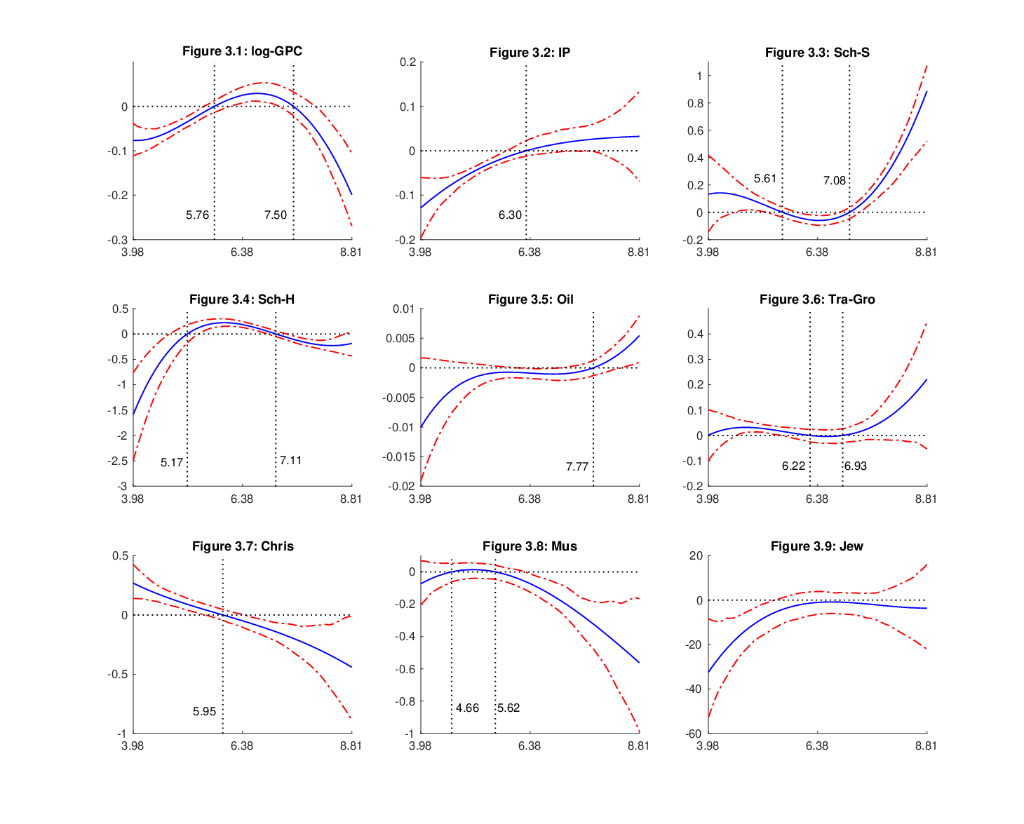
We now analyse some of the variables that are “significantly” related to growth in more details. Figure 3.1 presents our estimate of the coefficient of initial GDP per capita. This figure reveals three findings. First, this estimate is negative for most GDP per capita levels, thus being largely consistent with findings in the existing conditional convergence literature as well as previous studies that have employed model averaging methods to growth. Second, the coefficient has an inverse U-shaped relationship with initial GDP per capita. This finding is consistent with those reported by previous studies. For example, Durlauf et al. 2001 find that the coefficient of initial GDP per capita does not exhibit any sort of monotonicity with respect to level of development; Salimans 2012 finds that the coefficient of initial GDP per capita first increases with level of development up to a point and then declines afterwards; and Durlauf and Johnson 1995 find that the coefficient of initial GDP per capita is not monotonic with respect either GDP per capita or literacy rate. Third, the coefficient is positive for countries with GDP per capita between $319 and $1,812 in 1960 U.S. dollars (or between $2,554 and $14,510 in 2014 U.S. dollars), suggesting that some of these countries have been unable to catch up with more developed countries. This finding is in line with the “middle-income trap” hypothesis, which refers to the phenomenon of hitherto rapidly growing economies stagnating at middle-income levels and failing to graduate into the ranks of high-income countries (e.g., Eichengreen et al. 2014). In our sample South Africa and Columbia are two example countries that have never been able leave the “middle-income range” over the entire sample period since their GDP per capita fell into this range at the beginning of the sample period (i.e., 1960).

Figure 3.2 shows our estimate of the coefficient of price for investment goods. Three findings emerge from this figure. First, this estimate is negative for countries with initial GDP per capita up to $543 in 1960 U.S. dollars (or $4,348 in 2014 U.S. dollars), suggesting that for these countries a relative low price of investment goods in the first year of each five-year period is strongly and positively related to subsequent income growth. This finding is not surprising because a low investment price stimulates investment (including investment in machinery and equipment), which further spurs economic growth (De Long and Summers 1991; De Long and Summers 1992). Second, the estimated coefficient falls in absolute value as initial GDP per capita increases, meaning that the marginal effect of investment price on growth is stronger for poor countries than for rich countries. This latter finding is consistent with Temple 1999 who find that the growth-spurring effects of investment is greater for developing countries, because total investment includes machinery embodying well-established technologies and developing countries may be able to take advantage of new and old equipment because they have little of any technology. Third, for countries with initial GDP per capita above $543 in 1960 U.S. dollars (or $4,348 in 2014 U.S. dollars) the estimated coefficient of investment goods price is positive but insignificant, because the associated confidence intervals contain zero. This suggests that investment goods price has no growth effects for these countries. A possible reason for this latter finding is that the data from the Penn World Table is not disaggregated enough to distinguish price of equipment investment, which has strong growth effects, and price of other forms of investment, which have little growth effects (De Long and Summers 1991).

Figure 3.3 shows our estimate of the coefficient of secondary schooling enrolment. As this figure shows, this estimate is positive for most levels of initial GDP per capita. This is not surprising because secondary education is a vital part of a virtuous circle of economic growth within the context of a globalized knowledge economy. Many studies have documented that a large pool of workers with secondary education is indispensable for knowledge spillover to take place and for attracting imports of technologically advanced goods and foreign direct investment (Borensztein et al. 1998; Caselli and Coleman II 2001). That said, we also note that the estimated coefficient for secondary schooling is negative for middle income countries with initial GDP per capita between $272 and $1,192 in 1960 U.S. dollars (or between $2178 and $9,545 in 2014 U.S. dollars). This result suggests that a possible reason for the “middle income trap” discussed above is that these middle income countries, unlike other countries, fail to take advantage of the benefits brought by secondary schooling.

We also note from Figure 3.4 that the estimate of the coefficient of higher education is negative for almost all countries with the exception of middle income countries. This finding is consistent with Sala-I-Martin et al. 2004 and Salimans 2012, both of which find that the higher schooling coefficient is negative for most of their sample countries but positive for the rest. It also parallels the concavity argument that the earnings function is concave in education, meaning that returns are higher for lower levels of education (Psacharopoulos 1994; Psacharopoulos and Patrinos 2004).

Figure 3.5 shows our estimate of the coefficient of oil reserve. Two findings stand out from this figure. First, this estimate is negative for countries with initial GDP per capita below $2,373 in 1960 U.S. dollars (or $19,002 in 2014 U.S. dollars). This finding is consistent with the “natural resources curse hypothesis” (e.g., Sachs and Warner 2001) and can be explained by the rent-seeking behaviour of countries with large endowments of natural resources. Second, the oil reserve coefficient increases monotonically with GDP per capita and eventually becomes positive for economies with initial GDP per capita above $2,373 in 1960 U.S. dollars (or $19,002 in 2014 U.S. dollars). This latter finding accords with recent studies (e.g., Leite and Weidmann 1999) on the nexus between natural resources and economic growth. Specifically, these studies suggest that the contribution of natural resources to a country’s economy does not take place in isolation, but rather in the overall context of the country’s economic management and institutions. It is thus the quality and competency of these policies and institutions that will determine whether natural resources can promote economic growth, or whether revenues generated by the sector might impede development. Therefore, in developed economies where economic institutions are generally well-developed, natural resources tend to promote economic growth; whereas in developing economies where economic institutions are generally weak, natural resources tend to hamper economic growth.

Figure 3.6 presents the estimate of the coefficient of terms of trade growth. As this figure shows, our estimate of the terms of trade growth coefficient is positive for all countries, suggesting that growth tends to be faster in countries where the rate of change of terms of trade is higher. This finding is consistent with previous studies (Mendoza 1995; Mendoza 1997; Kose and Riezman 2001; Bleaney and Greenaway 2001) that find that an improvement in the terms of trade leads to higher levels of investment, and hence long-run economic growth. In addition, this figure shows that the terms of trade growth coefficient increases with GDP per capita, indicating that the marginal effect of terms of trade growth is larger in richer countries than in poorer ones. This latter finding is also consistent with previous studies (e.g., Blattman et al. 2007). Specifically, those studies argue that higher volatility in the terms of trade reduces investment and hence growth because of aversion to risk, and that rich countries with more sophisticated institutions and markets are likely to have cheaper ways to insure against price volatility than poor countries, so terms of trade instability is likely to have a smaller negative impact on rich countries.

Here we note that as in Sala-I-Martin et al. 2004, trade openness (defined as exports plus imports as a share of GDP) is insignificant, presumably reflecting the crudity of this measure, and perhaps the distinction between opening to international trade generating a one-time step increase in income as factors are reallocated according to comparative advantage versus an ongoing growth impact associated with greater openness.

Figures 3.7-3.9 show the estimates of the coefficients of fraction of Christian, Muslim, and Jewish respectively. These coefficients are negative at all levels of development or nearly all levels of development. This finding is consistent with that of Barro and McCleary 2005 who find that religion works via belief, not practice. They argue that higher church attendance uses up time and resources and eventually runs into diminishing returns. The “religion sector”, as they call it, can consume more than it yields.

6 Conclusion

A rigorous cross-country growth regression analysis should simultaneously account for three major problems identified in the literature — variable selection, parameter heterogeneity, and cross-sectional dependence. Though these three problems have received individual attention, little or no research has sought to integrate them into a single, comprehensive framework. The purpose of this study is to fill this void by proposing a new, integrated framework that is capable of dealing with parameter heterogeneity and cross-sectional dependence, while simultaneously performing variable selection. Specifically, parameter heterogeneity is allowed for by means of a varying coefficient growth regression model, while cross-sectional dependence is introduced into the model via a multi-factor structure. For simplicity, we refer to the resulting growth regression model as the “varying coefficient growth regression model with factor structure and sparsity”. We then propose a LASSO estimator that is capable of performing variable selection on this model. In addition, we have established the associated asymptotic results for this estimator and further investigate the performance of the estimator by conducting extensive simulations.

We apply the above framework to a new dataset that covers 89 countries over the period from 1960 to 2014. We have identified 31 robust growth determinants, providing evidentiary support for the canonical neoclassical growth variables; i.e., initial income, investment, and population growth, as well as macroeconomic policies, geography, institutions, religion and ethnic fractionalization. Moreover, we find that all the coefficients of the robust growth determinants vary considerably across countries according to their level of development, which reveals some interesting cross-country patterns not found in previous studies. For example, we find that the coefficient of the initial GDP per capita is positive for countries with GDP per capita between $319 and $1,812 in 1960 U.S. dollars (or between $2,554 and $14,510 in 2014 U.S. dollars), suggesting that some of these countries have fallen into the so-called “middle income trap”. As another example, we find that the oil reserve coefficient increases monotonically with GDP per capita and eventually becomes positive for economies with initial GDP per capita above $2,373 in 1960 U.S. dollars (or $19,002 in 2014 U.S. dollars), thus being consistent with recent studies that stress the role of institutions in determining how natural resources affect economic growth.

References

  • (1)
  • Ando and Bai (2017) Ando, T. and Bai, J. (2017), ‘Clustering huge number of financial time series: A panel data approach with high-dimensional predictors and factor structures’, Journal of the American Statistical Association 112(519), 1182–1198.
  • Attanasio et al. (2000) Attanasio, O. P., Picci, L. and Scorcu, A. E. (2000), ‘Saving, growth, and investment: A macroeconomic analysis using a panel of countries’, Review of Economics and Statistics 82(2), 182–211.
  • Bai (2009) Bai, J. (2009), ‘Panel data models with interactive fixed effects’, Econometrica 77(4), 1229–1279.
  • Barro (1991) Barro, R. J. (1991), ‘Economic growth in a cross section of countries’, Quarterly Journal of Economics 106(2), 407–443.
  • Barro and McCleary (2005) Barro, R. J. and McCleary, R. M. (2005), ‘Which countries have state religions?’, Quarterly Journal of Economics 120(4), 1331–1370.
  • Bernstein (2005) Bernstein, D. S. (2005), Matrix Mathematics: Theory, Facts, and Formulas, Princeton University Press.
  • Bils and Klenow (2000) Bils, M. and Klenow, P. J. (2000), ‘Does schooling cause growth?’, American Economic Review 90(5), 1160–1183.
  • Blattman et al. (2007) Blattman, C., Hwang, J. and Williamson, J. G. (2007), ‘The impact of the terms of trade on economic development in the periphery, 1870-1939: Volatility and secular change’, Journal of Development Economics 82(1), 156–179.
  • Bleaney and Greenaway (2001) Bleaney, M. and Greenaway, S. D. (2001), ‘The impact of terms of trade and real exchange rate volatility on investment and growth in sub-saharan africa’, Journal of Development Economics 65(2), 491–500.
  • Borensztein et al. (1998) Borensztein, E., De Gregorioand, J. and Lee, J. (1998), ‘How does foreign direct investment affect economic growth?’, Journal of International Economics 45(1), 115–135.
  • Brock and Durlauf (2001) Brock, W. A. and Durlauf, S. N. (2001), ‘Discrete choice with social interactions’, Review of Economic Studies 68(2), 235–260.
  • Caselli and Coleman II (2001) Caselli, F. and Coleman II, W. J. (2001), ‘The U.S. structural transformation and regional convergence: A reinterpretation’, Journal of Political Economy 109(3), 584–616.
  • Chen et al. (2012) Chen, J., Gao, J. and Li, D. (2012), ‘Semiparametric trending panel data models with cross–sectional dependence’, Journal of Econometrics 171(1), 71–85.
  • Chudik et al. (2017) Chudik, A., Mohaddes, K., Pesaran, M. H. and Raissi, M. (2017), ‘Is there a debt-threshold effect on output growth?’, Review of Economics and Statistics 99(1), 135–150.
  • Chudik et al. (2011) Chudik, A., Pesaran, M. H. and Tosetti, E. (2011), ‘Weak and strong cross-section dependence and estimation of large panels’, Econometrics Journal 14(1), C45–C90.
  • Connor et al. (2012) Connor, G., Hagmann, M. and Linton, O. (2012), ‘Efficient semiparametric estimation of the fama-french model and extensions’, Econometrica 80(2), 713–754.
  • De Long and Summers (1991) De Long, J. B. and Summers, L. (1991), ‘Equipment investment and economic growth’, The Quarterly Journal of Economics 106(2), 445–502.
  • De Long and Summers (1992) De Long, J. B. and Summers, L. (1992), ‘Equipment investment and economic growth: How strong is the nexus?’, Brookings Papers on Economic Activity 2, 157–199.
  • Dong et al. (2017) Dong, C., Gao, J. and Linton, O. (2017), High dimensional semiparametric moment restriction models. https://ssrn.com/abstract=3045063.
  • Dong et al. (2018) Dong, C., Gao, J. and Peng, B. (2018), Varying-coefficient panel data models with partially observed factor structure. https://ssrn.com/abstract=3102631.
  • Dong and Linton (2018) Dong, C. and Linton, O. (2018), ‘Additive nonparametric models with time variable and both stationary and nonstationary regressors’, Journal of Econometrics 207(1), 212–236.
  • Durlauf and Johnson (1995) Durlauf, S. N. and Johnson, P. A. (1995), ‘Multiple regimes and cross‐country growth behaviour’, Journal of Applied Econometrics 10(4), 365–384.
  • Durlauf et al. (2005) Durlauf, S. N., Johnson, P. A. and Temple, J. R. (2005), ‘Growth econometrics’, Handbook of Macroeconomics 1, Part A, 555–677.
  • Durlauf et al. (2001) Durlauf, S. N., Kourtellos, A. and Minkin, A. (2001), ‘The local solow growth model’, European Economic Review 45(4-6), 928–940.
  • Durlauf et al. (2008) Durlauf, S. N., Kourtellos, A. and Tan, C. M. (2008), ‘Are any growth theories robust’, Economic Journal 118(527), 329–346.
  • Durlauf and Quah (1999) Durlauf, S. N. and Quah, D. T. (1999), ‘The new empirics of economic growth’, Handbook of Macroeconomics 1, Part A, 235–308.
  • Eberhardt and Teal (2011) Eberhardt, M. and Teal, F. (2011), ‘Econometrics for grumblers: A new look at the literature on cross-country growth empirics’, Journal of Economic Surveys 25(1), 109–155.
  • Eichengreen et al. (2014) Eichengreen, B., Park, D. and Shin, K. (2014), ‘Growth slowdowns redux: New evidence on the middle-income trap’, Japan and the World Economy 32, 65–84.
  • Fan et al. (2016) Fan, J., Liao, Y. and Wang, W. (2016), ‘Projected Principal Component Analysis in Factor Models’, Annals of Statistics 44(1), 219–254.
  • Feng et al. (2017) Feng, G., Gao, J., Peng, B. and Zhang, X. (2017), ‘A varying-coefficient panel data model with fixed effects: theory and an application to the US commercial banks’, Journal of Econometrics 196(1), 68–82.
  • Fernández et al. (2001) Fernández, C., Ley, E. and Steel, M. F. J. (2001), ‘Model uncertainty in cross‐country growth regressions’, Journal of Applied Econometrics 16(5), 563–576.
  • Gao (2007) Gao, J. (2007), Nonlinear Time Series: Sem– and Non–Parametric Methods, Chapman & Hall/CRC.
  • Gao et al. (2018) Gao, J., Xia, K. and Zhu, H. (2018), ‘Heterogeneous panel data models with cross-sectional dependence’, Journal of Econometrics p. forthcoming.
  • Gill and Kharas (2007) Gill, I. and Kharas, H. (2007), An East Asian Renaissance : Ideas for Economic Growth, Washington, DC: World Bank.
  • Hall et al. (2007) Hall, P., Li, Q. and Racine, J. S. (2007), ‘Nonparametric estimation of regression functions in the presence of irrelevant regressors’, Review of Economics and Statistics 89(4), 784–789.
  • Huang et al. (2008) Huang, J., Horowitz, J. L. and Ma, S. (2008), ‘Asymptotic properties of bridge estimators in sparse high-dimensional regression models’, Annals of Statistics 36(2), 587–613.
  • Jiang et al. (2017) Jiang, B., Yang, Y., Gao, J. and Hsiao, C. (2017), Recursive estimation in large panel data models: Theory and practice. Working paper available at https://ssrn.com/abstract=2915749.
  • Kapetanios et al. (2011) Kapetanios, G., Pesaran, M. H. and Yamagata, T. (2011), ‘Panels with non-stationary multifactor error structures’, Journal of Econometrics 160(2), 326–348.
  • Kormendi and Meguire (1985) Kormendi, R. C. and Meguire, P. G. (1985), ‘Macroeconomic determinants of growth: Cross-country evidence’, Journal of Monetary Economics 16(2), 141–163.
  • Kose and Riezman (2001) Kose, A. and Riezman, R. (2001), ‘Trade shocks and macroeconomic fluctuations in africa’, Journal of Development Economics 65(1), 55–80.
  • Leamer (1983) Leamer, E. (1983), ‘Let’s take the con out of econometrics’, American Economic Review 73(1), 31–43.
  • Leite and Weidmann (1999) Leite, C. and Weidmann, J. (1999), Does mother nature corrupt? natural resources, corruption, and economic growth. IMF Working paper 99/85.
  • Li et al. (2016) Li, D., Qian, J. and Su, L. (2016), ‘Panel data models with interactive fixed effects and multiple structural breaks’, Journal of the American Statistical Association 111(516), 1804–1819.
  • Liu et al. (2018) Liu, F., Gao, J. and Yang, Y. (2018), Nonparametric time-varying panel data models with heterogeneity. https://ssrn.com/abstract=3214046.
  • Liu and Stengos (1999) Liu, Z. and Stengos, T. (1999), ‘Non-linearities in cross-country growth regressions: A semiparametric approach’, Journal of Applied Econometrics 14(5), 527–538.
  • Lu and Su (2016) Lu, X. and Su, L. (2016), ‘Shrinkage estimation of dynamic panel data models with interactive fixed effects’, Journal of Econometrics 190(1), 148–175.
  • Lucas (1993) Lucas, R. (1993), ‘Making a miracle’, Econometrica 61(2), 251–72.
  • Malikov et al. (2016) Malikov, E., Kumbhakar, S. C. and Sun, Y. (2016), ‘Varying coefficient panel data model in the presence of endogenous selectivity and fixed effects’, Journal of Econometrics 190(2), 233–251.
  • Mankiw et al. (1992) Mankiw, N. G., Romer, D. and Weil, D. N. (1992), ‘A contribution to the empirics of economic growth’, Quarterly Journal of Economics 107(2), 407–437.
  • Mendoza (1995) Mendoza, E. G. (1995), ‘The terms of trade, the real exchange rate, and economic fluctuations’, International Economic Review 36(1), 101–137.
  • Mendoza (1997) Mendoza, E. G. (1997), ‘Terms-of-trade uncertainty and economic growth’, Journal of Development Economics 54(2), 323–356.
  • Minier (2007) Minier, J. (2007), ‘Nonlinearities and robustness in growth regressions’, American Economic Review 97(2), 388–392.
  • Moral-Benito (2012) Moral-Benito, E. (2012), ‘Determinants of economic growth: A bayesian panel data approach’, Review of Economics and Statistics 94(2), 566–579.
  • Newey (1997) Newey, W. K. (1997), ‘Convergence rates and asymptotic normality for series estimators’, Journal of Econometrics 79(1), 147–168.
  • Pedroni (2007) Pedroni, P. (2007), ‘Social capital, barriers to production and capital shares: implications for the importance of parameter heterogeneity from a nonstationary panel approach’, Journal of Applied Econometrics 22(2), 326–348.
  • Pesaran (2006) Pesaran, M. H. (2006), ‘Estimation and inference in large heterogeneous panels with a multifactor error structure’, Econometrica 74(4), 967–1012.
  • Psacharopoulos (1994) Psacharopoulos, G. . (1994), ‘Returns to investment in education: A global update’, World Development 22(9), 1325–1343.
  • Psacharopoulos and Patrinos (2004) Psacharopoulos, G. and Patrinos, H. A. (2004), ‘Returns to investment in education: a further update’, Education Economics 12(2), 111–134.
  • Sachs and Warner (2001) Sachs, J. D. and Warner, A. (2001), ‘The curse of natural resources’, European Economic Review 45(4-6), 827–838.
  • Sala-I-Martin (1997) Sala-I-Martin, X. (1997), ‘I just ran two million regressions’, American Economic Review 87(2), 178–183.
  • Sala-I-Martin et al. (2004) Sala-I-Martin, X., Doppelhofer, G. and Miller, R. I. (2004), ‘Determinants of long-term growth: A bayesian averaging of classical estimates (bace) approach’, American Economic Review 94(4), 813–835.
  • Salimans (2012) Salimans, T. (2012), ‘Variable selection and functional form uncertainty in cross-country growth regressions’, Journal of Econometrics 171(2), 267–280.
  • Soto (2003) Soto, M. (2003), ‘Taxing capital flows: an empirical comparative analysis’, Journal of Development Economics 72(1), 203–221.
  • Su and Jin (2012) Su, L. and Jin, S. (2012), ‘Sieve estimation of panel data models with cross section dependence’, Journal of Econometrics 169(1), 34–47.
  • Su et al. (2015) Su, L., Jin, S. and Zhang, Y. (2015), ‘Specification test for panel data models with interactive fixed effects’, Journal of Econometrics 186(1), 222–244.
  • Summers and Heston (1991) Summers, R. and Heston, A. (1991), ‘The Penn World Table (Mark 5): an expanded set of international comparisons, 1950-1988’, Quarterly Journal of Economics 106(2), 327–368.
  • Temple (1999) Temple, J. (1999), ‘The new growth evidence’, Journal of Economic Literature 37(1), 112–156.
  • Wang and Xia (2009) Wang, H. and Xia, Y. (2009), ‘Shrinkage estimation of the varying coefficient’, Journal of the American Statistical Association 104(486), 747–757.
Table 1: Definitions of All Variables in the Regression
Variables Description Formula Mean Std
EG Economic growth rate ln(rgdpot/rgdpot-1) 0.0363 0.0649
log(GPC) log GDP per capita 6.0642 0.9861
csh_g Government consumption share 0.2074 0.1163
Openness Openness measure csh_x + csh_m -0.0322 0.1274
IP Investment price, i.e., price level of capital formation 0.4213 0.3220
PGR Population growth rates ln(popt/popt-1) 0.0197 0.0127
Sch_P Primary school enrollment 0.7396 0.2170
Sch_S Secondary school enrollment 0.4672 0.3204
Sch_H Higher education School Enrollment 0.1336 0.1581
LE Life Expecancy 0.5932 0.1102
PESS Public education spending share in GDP 0.0399 0.0296
PIS Public investment share GFCF - GFCF_PS 0.0713 0.0501
Land Land area (sq. km / 1,000,000) 0.8719 2.1518
Exports Percentage of Primary Export Exports_OM + Exports_ARM 0.1978 0.2085
Mining Fraction GDP in mining 0.0733 0.0874
Fertility Fertility rate, total (births per woman) 4.7412 1.9724
Military Military expenditure share in GDP 0.0295 0.0302
PCS Public consumption share GGFCE - PESS - Military 0.0809 0.0501
Malaria Malaria prevalence: Incidence of malaria 155.1712 245.5145
(per 1,000 population at risk)
Inflation Inflation rate 1.3854 7.0448
Political Political rights 4.2100 1.9429
Civil Civil liberties 4.1496 1.6628
Cap Degree of capitalism 3.2697 1.7275
Trade Terms of trade 1.3475 2.2807
Tra_Gro Terms of trade growth 0.0073 0.0974
Locked Landlocked country dummy (1, yes; 0, no) 0.2697 0.4438
Ind_Year Time of independence 1.4382 1.0382
<=1914 = 0; 1915-1945 = 1; 1946-1989 = 2; >= 1990 = 3
kgatr Percentage of land area in Koeppen-Geiger tropics 0.4017 0.4205
kgptr Percentage of population in Koeppen-Geiger tropics 0.3915 0.4217
lcr100km Percentage of Land area within 100 km of ice-free coast 0.3788 0.3640
pop100cr Ratio of population within 100 km of ice-free 0.4520 0.3728
coast/navigable river to total population
cen_lat latitude of country centroid 0.1522 0.2197
Bri_Col British colony dummy (1, yes; 0, no) 0.2584 0.4378
Spa_Col Spanish colony dummy (1, yes; 0, no) 0.1910 0.3931
Oil_OPEC Oil-producing country dummy (1, yes; 0, no) 0.0674 0.2508
Gas proved reserves (cubic meters / 10^12) 1.3789 6.1997
Oil proved reserves (bbl / 10^9) 4.5521 19.1378
Chris Percentage of Christian 0.5369 0.3807
Mus Percentage of Muslim 0.3046 0.3825
Hin Percentage of Hindu 0.0263 0.1211
Bud Percentage of Buddhist 0.0410 0.1541
Fol Percentage of Folk religion 0.0284 0.0628
Oth Percentage of other religion 0.0037 0.0064
Jew Percentage of Jewish 0.0019 0.0027
GS Government spending share of GDP 0.1501 0.0686
Distortion Real exchange rate distortions 129.6824 35.8479
OO Outward orientation -2.7398 0.7542
SIL Ethnolinguistic fractionalization 0.4886 0.3127
ESP English-speaking population in percentage 0.1762 0.2692
EA East Asian dummy 0.0225 0.1482
AF African dummy 0.4270 0.4947
EU European dummy 0.1124 0.3158
LA Latin American dummy 0.1573 0.3641
WarFrac Fraction spent in war (1960-2014) 0.3265 0.4343
NoWars No. of war participation (1960-2014) 0.8028 1.2609
Coup coups d’etat and coup attempts within (1960-2014) 0.1870 0.4964
Revolution Number of revolutions (1960-2014) 0.1941 0.5038
Pop_Dens Population Density/1000 0.0812 0.1135
WorkIR Growth rate of work force ln(WPt/WPt-1) 0.0210 0.0132
rgdpo — Size of economy (GDP in million)
pop — Population (in million)
csh_x — Share of merchandise exports
csh_m — Share of merchandise imports
WP — Fraction population of work force (1-A65-U15)
A65 — Fraction population over 65 years old
U15 — Fraction population under 15 years old
GFCF — Gross fixed capital formation
GFCF_PS — Gross fixed capital formation, private sector
Exports_OM — Percentage of Ores and metals exports
Exports_ARM — Percentage of Agricultural raw materials exports
GGFCE — General government final consumption expenditure share in GDP
Table 2: Sample Countries and Their Associated ISO 3166-1 alpha-3 Codes
AGO Angola HND Honduras PAK Pakistan
ALB Albania HRV Croatia PAN Panama
ARM Armenia HTI Haiti PER Peru
AZE Azerbaijan IND India PHL Philippines
BDI Burundi IRN Iran, Islamic Republic of POL Poland
BEN Benin JAM Jamaica PRY Paraguay
BFA Burkina Faso JOR Jordan RUS Russian Federation
BGD Bangladesh JPN Japan RWA Rwanda
BGR Bulgaria KAZ Kazakhstan SDN Sudan
BLR Belarus KEN Kenya SEN Senegal
BRA Brazil KGZ Kyrgyzstan SLE Sierra Leone
BWA Botswana KHM Cambodia SLV El Salvador
CAF Central African Republic LAO Lao People’s Democratic Republic SWZ Swaziland
CIV Côte d’Ivoire LBN Lebanon SYR Syrian Arab Republic
CMR Cameroon LKA Sri Lanka TCD Chad
COG Congo LSO Lesotho TGO Togo
COL Colombia MDA Moldova, Republic of THA Thailand
DOM Dominican Republic MDG Madagascar TTO Trinidad and Tobago
DZA Algeria MEX Mexico TUN Tunisia
ECU Ecuador MKD Macedonia TUR Turkey
EGY Egypt MLI Mali TZA Tanzania, United Republic of
ETH Ethiopia MNG Mongolia UGA Uganda
GAB Gabon MOZ Mozambique UKR Ukraine
GBR United Kingdom MWI Malawi URY Uruguay
GEO Georgia MYS Malaysia USA United States
GHA Ghana NAM Namibia VEN Venezuela, Bolivarian Republic of
GIN Guinea NER Niger YEM Yemen
GMB Gambia NIC Nicaragua ZAF South Africa
GNB Guinea-Bissau NPL Nepal ZWE Zimbabwe
GTM Guatemala OMN Oman
Table 3: Comparison among Alternative Development Indexes (zz)
Parametric zz of Varying Coefficient
ln\ln(GPC) School_P School_S School_H
RMSE 0.022 0.017 0.019 0.027 0.020
No. of factors 6 6 6 3 5
Table 4: Cumulative Variation of the Residuals Explained by the Factors
No. Factors 1 2 3 4 5 6
Cumulative Variation 87.86% 94.87% 96.65% 98.10% 98.71% 99.01%
Table 5: Estimates of Coefficients at log(GPC)=3.98, 5, 6, 7, 8 and 8.81
log(GPC)=3.98 log(GPC)=5 log(GPC)=6 log(GPC)=7 log(GPC)=8 log(GPC)=8.81
log(GPC) -0.0766 -0.0447 0.0117 0.0255 -0.0531 -0.2055
(-0.1145, -0.0429) (-0.0618, -0.0305) (-0.0038, 0.0249) (0.0080, 0.0469) (-0.0886, -0.0034) (-0.2883, -0.0898)
csh_g 0.3341 0.1483 -0.0587 -0.2143 -0.2619 -0.1964
(0.1077, 0.5534) (0.0706, 0.2248) (-0.1110, -0.0107) (-0.3141, -0.1454) (-0.5782, 0.0082) (-0.9416, 0.4733)
IP -0.1284 -0.0545 -0.0093 0.0160 0.0282 0.0325
(-0.1971, -0.0621) (-0.0686, -0.0422) (-0.0191, 0.0059) (-0.0046, 0.0406) (-0.0146, 0.0638) (-0.0895, 0.1209)
PGR 3.2821 0.5353 0.8485 1.5689 0.6502 -2.2853
(1.7325, 4.7072) (0.0426, 0.9486) (0.4054, 1.2542) (1.1371, 1.9781) (-0.1228, 1.3620) (-3.5441, -0.7206)
School_S 0.1322 0.0823 -0.0420 -0.0147 0.3303 0.9119
(-0.1505, 0.4845) (0.0108, 0.1495) (-0.0780, -0.0081) (-0.0548, 0.0177) (0.1989, 0.4201) (0.5495, 1.1719)
School_H -1.5869 -0.1175 0.2220 0.0326 -0.2066 -0.1808
(-2.4454, -0.7631) (-0.3214, 0.1119) (0.1562, 0.3020) (-0.0157, 0.0921) (-0.2810, -0.1039) (-0.3986, 0.1401)
LE 0.3148 0.2935 -0.0597 -0.2370 0.1455 1.0373
(-0.0171, 0.6403) (0.1811, 0.3938) (-0.1739, 0.0389) (-0.3918, -0.0990) (-0.2875, 0.5411) (0.0000, 1.9922)
PESS -1.2399 -0.5737 -0.2476 -0.0158 0.3070 0.7260
(-2.4950, 0.0107) (-0.7969, -0.3513) (-0.4210, -0.0944) (-0.2163, 0.1716) (-0.6249, 1.3302) (-1.5776, 3.4530)
Military -1.1748 -0.1436 -0.0428 -0.0020 0.6417 1.9197
(-2.4253, -0.0639) (-0.3588, 0.1047) (-0.1667, 0.0719) (-0.2609, 0.1609) (0.0134, 1.1085) (0.1982, 3.4369)
Inflation -0.0055 0.0006 -0.0011 -0.0031 0.0007 0.0107
(-0.0094, -0.0012) (0.0000, 0.0012) (-0.0016, -0.0005) (-0.0039, -0.0023) (-0.0043, 0.0048) (-0.0020, 0.0209)
Civil 0.0183 0.0050 -0.0004 0.0033 0.0166 0.0340
(0.0048, 0.0308) (0.0011, 0.0085) (-0.0027, 0.0024) (0.0000, 0.0064) (0.0027, 0.0282) (-0.0036, 0.0661)
Tra_Gro 0.0009 0.0304 0.0048 0.0018 0.0796 0.2279
(-0.1138, 0.1100) (0.0117, 0.0458) (-0.0162, 0.0252) (-0.0248, 0.0351) (-0.0062, 0.1727) (-0.0124, 0.4799)
kgatr -0.3099 -0.0815 -0.0763 -0.1422 -0.1597 -0.0776
(-0.4367, -0.1693) (-0.1281, -0.0391) (-0.1161, -0.0447) (-0.1887, -0.0969) (-0.2602, -0.0333) (-0.3270, 0.2396)
lcr100km 0.6793 0.1930 0.0511 -0.0621 -0.3850 -0.9133
(0.5005, 0.8498) (0.1396, 0.2461) (0.0127, 0.0940) (-0.1305, -0.0005) (-0.5977, -0.2168) (-1.4617, -0.5189)
cen_lat 0.5894 0.0293 0.0360 0.1693 0.0873 -0.3058
(0.3011, 0.8198) (-0.0723, 0.1294) (-0.0315, 0.1114) (0.0985, 0.2655) (-0.0526, 0.2459) (-0.6344, 0.0789)
Spa_Col -0.5174 -0.1564 -0.0204 0.0548 0.1945 0.4167
(-0.6748, -0.3222) (-0.2111, -0.1080) (-0.0503, 0.0091) (0.0171, 0.0950) (0.1040, 0.3131) (0.1867, 0.6800)
Oil_OPEC -0.1254 -0.0460 -0.0947 -0.0815 0.1358 0.5247
(-1.0835, 0.6246) (-0.2325, 0.1181) (-0.1496, -0.0423) (-0.1383, -0.0344) (-0.0124, 0.2413) (0.1090, 0.8785)
Oil -0.0100 -0.0021 -0.0008 -0.0011 0.0008 0.0057
(-0.0217, 0.0018) (-0.0051, 0.0009) (-0.0017, 0.0000) (-0.0022, -0.0001) (-0.0010, 0.0023) (0.0004, 0.0099)
Chris 0.2689 0.1112 -0.0056 -0.1262 -0.2818 -0.4469
(0.1164, 0.4267) (0.0650, 0.1711) (-0.0535, 0.0461) (-0.2001, -0.0629) (-0.4824, -0.1333) (-0.8908, -0.0694)
Mus -0.0736 0.0130 -0.0292 -0.1685 -0.3744 -0.5692
(-0.1864, 0.0735) (-0.0383, 0.0599) (-0.0774, 0.0195) (-0.2344, -0.1004) (-0.5710, -0.2335) (-1.0085, -0.2474)
Oth -3.7386 0.6890 -1.1133 2.9016 21.6126 51.3537
(-13.0771, 4.1928) (-1.3860, 2.4081) (-3.0584, 0.7782) (0.2919, 6.3889) (11.6269, 32.3911) (27.3474, 75.2005)
Jew -32.4452 -10.5477 -2.0163 -0.9826 -2.7502 -3.6114
(-55.7335, -10.0679) (-18.6022, -3.8609) (-7.6269, 3.6243) (-6.9105, 4.0461) (-12.1471, 5.8912) (-27.3730, 18.2231)
GS -0.2516 -0.2079 -0.0476 -0.0738 -0.5101 -1.2583
(-0.5709, 0.0529) (-0.3047, -0.1254) (-0.1142, 0.0215) (-0.1676, 0.0172) (-0.8230, -0.1881) (-2.1023, -0.4396)
Distortion 0.0231 0.0884 0.1085 0.0482 -0.1148 -0.3280
(-0.0449, 0.1048) (0.0580, 0.1187) (0.0701, 0.1435) (-0.0064, 0.1025) (-0.2793, 0.0061) (-0.6718, -0.0148)
OO 1.0569 4.1811 5.1496 2.3016 -5.4384 -15.5641
(-2.1588, 4.9579) (2.7557, 5.6164) (3.3263, 6.8047) (-0.2707, 4.8851) (-13.1848, 0.3040) (-31.9253, -0.7429)
ESP 0.3819 0.1039 0.0581 0.1010 0.1193 0.0577
(0.2151, 0.5483) (0.0575, 0.1465) (0.0214, 0.0975) (0.0494, 0.1631) (-0.0059, 0.2319) (-0.2260, 0.2967)
EA 0.2924 0.0841 0.0263 -0.1256 -0.5515 -1.1753
(-0.1574, 0.7975) (-0.0589, 0.2081) (-0.0668, 0.1185) (-0.2975, 0.0293) (-1.0307, -0.1357) (-2.2484, -0.2191)
EU -1.0237 -0.2206 -0.0275 0.0738 0.4780 1.2174
(-1.7313, -0.3070) (-0.3896, -0.0438) (-0.0797, 0.0197) (0.0169, 0.1225) (0.3182, 0.6845) (0.7527, 1.7964)
WarFrac -0.0044 -0.0035 -0.0120 -0.0130 0.0058 0.0411
(-0.0372, 0.0351) (-0.0121, 0.0072) (-0.0179, -0.0040) (-0.0208, -0.0036) (-0.0157, 0.0235) (-0.0227, 0.0882)
Coup -0.0190 -0.0004 -0.0028 -0.0070 0.0016 0.0251
(-0.0287, -0.0089) (-0.0031, 0.0020) (-0.0051, -0.0005) (-0.0102, -0.0038) (-0.0086, 0.0113) (-0.0005, 0.0502)
Revolution -0.0052 0.0044 -0.0016 -0.0066 0.0021 0.0252
(-0.0198, 0.0090) (0.0007, 0.0075) (-0.0042, 0.0011) (-0.0106, -0.0020) (-0.0054, 0.0084) (-0.0034, 0.0464)
Figure 1: Estimates of Common Factors
Refer to caption

f^t,j\widehat{f}_{t,j} stands for the estimate of the jt​hj^{th} factor, where j=1​…,6j=1\ldots,6.

Figure 2: Estimates of Factor Loadings
Refer to caption

γ^i,j\widehat{\gamma}_{i,j} stands for the estimate of the jt​hj^{th} factor loading, where j=1​…,6j=1\ldots,6.

Figure 3: Estimates of Selected Coefficient Functions
Refer to caption

Supplementary Appendix A to
“An Integrated Panel Data Approach to
Modelling Economic Growth”

Guohua Feng∗, Jiti Gao♯ and Bin Peng†

∗University of North Texas, ♯Monash University and †University of Bath

Appendix A is divided into five sections. Section A.1 provides the numerical algorithm. Section A.2 examines the asymptotic results of Section 3 through several simulations. Section A.3 presents the preliminary lemmas and the proofs of the main theorems. Section A.4 explains why our method can partially solve the issue of time trend that has found limited attention in the empirical growth literature. In Section A.5, we provide auxiliary tables and figures of the empirical study.

Recall that in the main text, we have let ξN​T=min⁡{N,T}\xi_{NT}=\min\{N,T\}, ∥⋅∥sp\|\cdot\|_{\textrm{sp}} be the spectral norm of a matrix, and ⌊a⌋\lfloor a\rfloor stand for the largest integer part of a real number aa. Here we further define some notations, which will be used throughout this file. Let ϕi∗​[β∗]=(xi​1∗′​β∗​(zi​1),…,xi​T∗′​β∗​(zi​T))′\phi_{i}^{*}[\beta^{*}]=({x_{i1}^{*}}^{\prime}\beta^{*}(z_{i1}),\ldots,{x_{iT}^{*}}^{\prime}\beta^{*}(z_{iT}))^{\prime}, and ϕi†​[β†]=(xi​1†′​β†​(zi​1),…,xi​T†′​β†​(zi​T))′\phi_{i}^{\dagger}[\beta^{\dagger}]=({x_{i1}^{\dagger}}^{\prime}\beta^{\dagger}(z_{i1}),\ldots,{x_{iT}^{\dagger}}^{\prime}\beta^{\dagger}(z_{iT}))^{\prime}, where β∗​(⋅)\beta^{*}(\cdot) and β†​(⋅)\beta^{\dagger}(\cdot) are p∗×1p^{*}\times 1 and (p−p∗)×1(p-p^{*})\times 1 respectively. Moreover, diag​{A1,…,Ak}\textrm{diag}\{A_{1},\ldots,A_{k}\} means constructing block diagonal matrix from matrices (or scalars) A1,…,AkA_{1},\ldots,A_{k}.

A.1 Numerical Implementation

The following procedure essentially combines two algorithms discussed in Bai 2009 and Wang and Xia 2009 together. For each given λ=(λ1,…,λp)′\lambda=(\lambda_{1},\ldots,\lambda_{p})^{\prime}, the estimates can be obtained using the following iteration procedure. Let C^β(n)\widehat{C}_{\beta}^{(n)} and F^(n)\widehat{F}^{(n)} be the estimates obtained from the nt​h≥1n^{th}\geq 1 iteration. Then, for the (n+1)t​h(n+1)^{th} iteration, the estimates are obtained as

Sub-step 1:vec(C^β(n+1))=(∑i=1N𝒵i′MF^(n)𝒵i+Dm,p(n)2)−1∑i=1N𝒵i′MF^(n)Yi,\displaystyle\text{Sub-step 1:}\hskip 9.24994pt\vect(\widehat{C}_{\beta}^{(n+1)})=\left(\sum_{i=1}^{N}\mathcal{Z}_{i}^{\prime}M_{\widehat{F}^{(n)}}\mathcal{Z}_{i}+\frac{D_{m,p}^{(n)}}{2}\right)^{-1}\sum_{i=1}^{N}\mathcal{Z}_{i}^{\prime}M_{\widehat{F}^{(n)}}Y_{i},
Sub-step 2:1N​T∑i=1N(Yi−ϕi[β^m(n+1)])(Yi−ϕi[β^m(n+1)])′F^(n+1)=F^(n+1)VN​T,\displaystyle\text{Sub-step 2:}\hskip 9.24994pt\frac{1}{NT}\sum_{i=1}^{N}\left(Y_{i}-\phi_{i}[\widehat{\beta}_{m}^{(n+1)}]\right)\left(Y_{i}-\phi_{i}[\widehat{\beta}_{m}^{(n+1)}]\right)^{\prime}\widehat{F}^{(n+1)}=\widehat{F}^{(n+1)}V_{NT},

where Dm,p=Im⊗diag​{λ1‖C^β,1(n)‖,…,λp‖C^β,p(n)‖}D_{m,p}=I_{m}\otimes\text{diag}\left\{\frac{\lambda_{1}}{\|\widehat{C}_{\beta,1}^{(n)}\|},\ldots,\frac{\lambda_{p}}{\|\widehat{C}_{\beta,p}^{(n)}\|}\right\}; and VN​TV_{NT} is a diagonal matrix with the diagonal being the rr largest eigenvalues of

1N​T​∑i=1N(Yi−ϕi​[β^m(n+1)])​(Yi−ϕi​[β^m(n+1)])′\displaystyle\frac{1}{NT}\sum_{i=1}^{N}\left(Y_{i}-\phi_{i}[\widehat{\beta}_{m}^{(n+1)}]\right)\left(Y_{i}-\phi_{i}[\widehat{\beta}_{m}^{(n+1)}]\right)^{\prime}

arranged in descending order. We stop the iteration when the estimates reach certain criteria, say ‖C^β(n+1)−C^β(n)‖≤ϵ\|\widehat{C}_{\beta}^{(n+1)}-\widehat{C}_{\beta}^{(n)}\|\leq\epsilon. To start the above iteration, we randomly generate F^(0)\widehat{F}^{(0)}, where each element of F^(0)\widehat{F}^{(0)} follows from N⁡(0,1)N(0,1).

To choose the optimal λ\lambda, we follow Wang and Xia 2009 to simplify it as follows:

λ=ν​(‖C¯β,1‖−1,…,‖C¯β,p‖−1)′,\displaystyle\lambda=\nu\left(\|\bar{C}_{\beta,1}\|^{-1},\ldots,\|\bar{C}_{\beta,p}\|^{-1}\right)^{\prime}, (A.1.1)

where ν\nu is a scalar, and C¯β,j\bar{C}_{\beta,j} stands for the jt​hj^{th} row of the unregularized estimator C¯β\bar{C}_{\beta} (i.e., implementing (3.3) of the main text with λ=0p×1\lambda=0_{p\times 1}). With the specification of (A.1.1), the idea for choosing lambda becomes straightforward. The unregularized estimator C¯β\bar{C}_{\beta} is a consistent estimator. It provides information on how likely each row of Cβ0C_{\beta_{0}} is a zero row. In other words, smaller ‖C¯β,j‖\|\bar{C}_{\beta,j}\| implies that the jt​hj^{th} row of Cβ0C_{\beta_{0}} is more likely to be zero and hence suggests a larger regularizer on ‖Cβ,j‖\|C_{\beta,j}\|. Given (A.1.1), the selection on the vector λ\lambda reduces to the selection on the scalar ν\nu. Finally, we consider the possible value of ν\nu over a sufficiently large interval of the real line. The optimal ν\nu is chosen by minimizing the BIC type criteria proposed in the main text. For the HD case, ΥN​T\Upsilon_{NT} is chosen as ln⁡ξN​TξN​T8\frac{\ln\xi_{NT}}{\sqrt[8]{\xi_{NT}}} in view of the development of Lemma A.7 and Theorem 3.3.

A.2 A Numerical Study

In this section, we examine the performance of the methodology of Section 3 through several simulations. Consider the model (2.4) of the main text. For the factor structure, let f0​t∼i.i.d. ​N​(0r×1,Ir)f_{0t}\sim\text{i.i.d. }N(0_{r\times 1},I_{r}) and γ0​i∼i.i.d. ​N​(0.5⋅1r×1,Ir)\gamma_{0i}\sim\text{i.i.d. }N(0.5\cdot 1_{r\times 1},I_{r}). In order to generate the regressors and univariate index variable, we firstly generate vi​t=0.5⋅vi,t−1+ξi​tv_{it}=0.5\cdot v_{i,t-1}+\xi_{it}, where ξi​t∼i.i.d. ​N​(0p×1,Ip)\xi_{it}\sim\text{i.i.d. }N(0_{p\times 1},I_{p}). Then let xi​t=vi​t+|γ0​i′​f0​t|x_{it}=v_{it}+|\gamma_{0i}^{\prime}f_{0t}|, and zi​t=|vi​t,1|+i.i.d. ​N​(0,1)z_{it}=|v_{it,1}|+\text{i.i.d. }N(0,1), where vi​t,1v_{it,1} stands for the first element of vi​tv_{it}. By doing so, we generate certain correlation between the regressors and the factor structure, and also introduce some correlation between zi​tz_{it} and xi​tx_{it}. The error terms are generated as εt=0.5⋅εt−1+ζt\varepsilon_{t}=0.5\cdot\varepsilon_{t-1}+\zeta_{t} in which ζt∼i.i.d. ​N​(0N×1,Σζ)\zeta_{t}\sim\text{i.i.d. }N(0_{N\times 1},\Sigma_{\zeta}) and Σζ={0.5|i−j|}N×N\Sigma_{\zeta}=\{0.5^{|i-j|}\}_{N\times N}, so that the weak cross-sectional dependence among individuals, and serial correlation over time dimension are generated. For both LD and HD cases, the rest settings are as follows:

  • •

    LD Case: p∗=2p^{*}=2, p=5p=5, r=3r=3, and let β01(z)=exp(−z2/2)+0.4\beta_{01}(z)=\exp(-z^{2}/2)+0.4 and β02(z)=z⋅exp(−z2/2)+0.7\beta_{02}(z)=z\cdot\exp(-z^{2}/2)+0.7;

  • •

    HD Case: p∗=2⋅⌊1.2​(N​T)1/6⌋p^{*}=2\cdot\lfloor 1.2(NT)^{1/6}\rfloor, p=30p=30, r=3r=3. For j=1,…,p∗j=1,\ldots,p^{*}, β0​j(z)=exp(−z2/2)+0.4\beta_{0j}(z)=\exp(-z^{2}/2)+0.4 when jj is odd, and β0​j(z)=z⋅exp(−z2/2)+0.7\beta_{0j}(z)=z\cdot\exp(-z^{2}/2)+0.7 when jj is even.

For each dataset generated, we implement the procedure of Section 3 to perform variable selection first. After identifying 𝒜∗\mathcal{A}^{*} and 𝒜†\mathcal{A}^{\dagger}, we implement post-selection estimation (i.e., remove the irrelevant regressors and then implement (3.3) of the main text with λ=0p×1\lambda=0_{p\times 1}) for the coefficient functions. We adopt the Hermite functions of Dong and Linton 2018 as the basis functions, repeat the above procedure 1000 times, and let44 4 Note that the optimal choice of mm may not be the optimal one, but it satisfies all the requirements of our assumptions. Although the optimal choice of truncation parameter and the optimal bandwidth selection have been solved for some cross-sectional models and time series models (e.g., Gao 2007; Hall et al. 2007) under the low dimensional cases, it is well understood that the question is still open even for the nonparametric panel data model with fixed effects (cf., Chen et al. 2012; Su and Jin 2012). The question is even more daunting when the factor structure and variable selection procedure get involved. N∈{40, 80, 120}N\in\{40,\,80,\,120\}, T∈{40, 80, 120}T\in\{40,\,80,\,120\}, and m=⌊1.2​(N​T)1/6⌋m=\lfloor 1.2(NT)^{1/6}\rfloor.

To evaluate our simulation results, we firstly report two percentages: (1) the percentage of missed true regressors (i.e., false negative rate, FNR); and (2) the percentage of falsely selected noise regressors (i.e., false positive rate, FPR). Secondly, we evaluate the estimates on the components of β0​(⋅)\beta_{0}(\cdot). Take β01​(⋅)\beta_{01}(\cdot) as an example. For the jt​hj^{th} replication, we obtain β^1​j​(z)\widehat{\beta}_{1j}(z) for ∀z\forall z (given it is not identified as 0; otherwise, we record 0 as the estimate). For ∀z\forall z, we calculate β^1​(z)=11000​∑j=11000β^1​j​(z)\widehat{\beta}_{1}(z)=\frac{1}{1000}\sum_{j=1}^{1000}\widehat{\beta}_{1j}(z), and also record the 95% confidence bands based on {β^1​j(z)|j=1,…,1000}\{\widehat{\beta}_{1j}(z)\,|\,j=1,\ldots,1000\}. We plot these values over a certain range of zz. The values of β01​(z)\beta_{01}(z) are plotted in solid black line, and the values of β^1​(z)\widehat{\beta}_{1}(z) are plotted in red dotted line, and the associated 95% confidence bands are plotted in blue dashed curves.

Table A.1 summarizes the FNR and FPR for the LD and HD cases respectively. It is clear that our method proposed in Section 3 works well, as both FNR and FPR are either 0 or very close to 0. It is worth mentioning that although FPR is slightly higher than zero for the HD case, over selecting the regressors will still yield consistent estimation.

Table A.1: FNR & FPR
FNR FPR
N∖TN\setminus T 40 80 120 40 80 120
LD 40 0.00% 0.00% 0.00% 0.00% 0.00% 0.00%
40 0.00% 0.00% 0.00% 0.00% 0.00% 0.00%
120 0.00% 0.00% 0.00% 0.00% 0.00% 0.00%
HD 40 0.00% 0.00% 0.00% 9.90% 1.10% 1.60%
40 0.00% 0.00% 0.00% 1.70% 1.90% 1.20%
120 0.00% 0.00% 0.00% 3.60% 1.00% 0.80%

For both the LD and HD cases, we plot β01​(z)\beta_{01}(z) and β02​(z)\beta_{02}(z) on [−1,2][-1,2] in Figures A.1-A.4, as the majority of zi​tz_{it}’s lie in this range. Due to similarity, we do not report the estimates of the rest coefficient functions for HD case. It is easy to see that as the sample size increases, the 95% confidence bands become much narrower and the mean estimate approaches the true curve. Also, the estimates from the HD case have wider 95% confidence bands, and seem to be less accurate compared to the LD case as expected.

Refer to caption
Figure A.1: LD: β01(z)=exp(−z2/2)+0.4\beta_{01}(z)=\exp(-z^{2}/2)+0.4
Refer to caption
Figure A.2: LD: β02(z)=zexp(−z2/2)+0.7\beta_{02}(z)=z\exp(-z^{2}/2)+0.7
Refer to caption
Figure A.3: HD: β01(z)=exp(−z2/2)+0.4\beta_{01}(z)=\exp(-z^{2}/2)+0.4
Refer to caption
Figure A.4: HD: β02(z)=zexp(−z2/2)+0.7\beta_{02}(z)=z\exp(-z^{2}/2)+0.7

A.3 Proofs

Before proving the main theorems, we present the following preliminary lemmas.

Lemma A.1.

Consider two non-singular symmetric matrices A,BA,B with the same dimensions k×kk\times k, where kk tends to ∞\infty. Suppose that their minimum eigenvalues satisfy that ηmin​(A)>0\eta_{\text{min}}(A)>0 and ηmin​(B)>0\eta_{\text{min}}(B)>0 uniformly in kk. Then ‖A−1−B−1‖≤ηmin−1​(A)⋅ηmin−1​‖A−B‖\left\|A^{-1}-B^{-1}\right\|\leq\eta_{\text{min}}^{-1}\left(A\right)\cdot\eta_{\text{min}}^{-1}\left\|A-B\right\|.

Lemma A.2.

Let Assumptions 1 and 2 hold. As (N,T)→(∞,∞)(N,T)\to(\infty,\infty),

  1. 1.

    ‖1N​T​ℰ′​ℰ‖=OP​(1N)+OP​(1T)\|\frac{1}{NT}\mathcal{E}^{\prime}\mathcal{E}\|=O_{P}\left(\frac{1}{\sqrt{N}}\right)+O_{P}\left(\frac{1}{\sqrt{T}}\right) and ‖1N​T​ℰ​ℰ′‖=OP​(1N)+OP​(1T)\|\frac{1}{NT}\mathcal{E}\mathcal{E}^{\prime}\|=O_{P}\left(\frac{1}{\sqrt{N}}\right)+O_{P}\left(\frac{1}{\sqrt{T}}\right), where ℰ=(ℰ1,…,ℰN)′\mathcal{E}=(\mathcal{E}_{1},\ldots,\mathcal{E}_{N})^{\prime},

  2. 2.

    supF∈𝖣F1N​T​∑i=1Nℰi′​PF​ℰi=OP​(1N)+OP​(1T)\displaystyle\sup_{F\in\mathsf{D}_{F}}\frac{1}{NT}\sum_{i=1}^{N}\mathcal{E}_{i}^{\prime}P_{F}\mathcal{E}_{i}=O_{P}\left(\frac{1}{\sqrt{N}}\right)+O_{P}\left(\frac{1}{\sqrt{T}}\right),

  3. 3.

    supF∈𝖣F|1N​T​∑i=1Nγ0​i′​F0′​MF​ℰi|=OP​(1N4)+OP​(1T4)\displaystyle\sup_{F\in\mathsf{D}_{F}}\left|\frac{1}{NT}\sum_{i=1}^{N}\gamma_{0i}^{\prime}F_{0}^{\prime}M_{F}\mathcal{E}_{i}\right|=O_{P}\left(\frac{1}{\sqrt[4]{N}}\right)+O_{P}\left(\frac{1}{\sqrt[4]{T}}\right),

  4. 4.

    sup‖Cβ‖≤M,F∈𝖣F|1N​T​∑i=1N(ϕi​[β0,m]−ϕi​[βm])′​MF​ℰi|=OP​(1N4)+OP​(1T4)\displaystyle\sup_{\|C_{\beta}\|\leq M,\,F\in\mathsf{D}_{F}}\left|\frac{1}{NT}\sum_{i=1}^{N}\left(\phi_{i}[\beta_{0,m}]-\phi_{i}[\beta_{m}]\right)^{\prime}M_{F}\mathcal{E}_{i}\right|=O_{P}\left(\frac{1}{\sqrt[4]{N}}\right)+O_{P}\left(\frac{1}{\sqrt[4]{T}}\right),

  5. 5.

    supF∈𝖣F|1N​T​∑i=1Nϕi​[Δm]′​MF​ϕi​[Δm]|=OP​(m−μ)\displaystyle\sup_{F\in\mathsf{D}_{F}}\left|\frac{1}{NT}\sum_{i=1}^{N}\phi_{i}[\Delta_{m}]^{\prime}M_{F}\phi_{i}[\Delta_{m}]\right|=O_{P}\left(m^{-\mu}\right),

  6. 6.

    supF∈𝖣F|1N​T​∑i=1Nϕi​[Δm]′​MF​F0​γ0​i|=OP​(m−μ2)\displaystyle\sup_{F\in\mathsf{D}_{F}}\left|\frac{1}{NT}\sum_{i=1}^{N}\phi_{i}[\Delta_{m}]^{\prime}M_{F}F_{0}\gamma_{0i}\right|=O_{P}(m^{-\frac{\mu}{2}}),

  7. 7.

    sup‖Cβ‖≤M,F∈𝖣F|1N​T​∑i=1Nϕi​[Δm]′​MF​{ϕi​[βm]−ϕi​[β0,m]}|=OP​(m−μ2)\displaystyle\sup_{\|C_{\beta}\|\leq M,\,F\in\mathsf{D}_{F}}\left|\frac{1}{NT}\sum_{i=1}^{N}\phi_{i}\left[\Delta_{m}\right]^{\prime}M_{F}\left\{\phi_{i}\left[\beta_{m}\right]-\phi_{i}\left[\beta_{0,m}\right]\right\}\right|=O_{P}(m^{-\frac{\mu}{2}}),

where MM is a sufficiently large constant.

Let ΠN​T−1=VN​T​(F0′​F^/T)−1​(Γ0′​Γ0/N)−1\Pi_{NT}^{-1}=V_{NT}(F_{0}^{\prime}\widehat{F}/T)^{-1}(\Gamma_{0}^{\prime}\Gamma_{0}/N)^{-1}, where VN​TV_{NT} is a diagonal matrix with the diagonal being the rr largest eigenvalues of

1N​T​∑i=1N(Yi−ϕi​[β^m])​(Yi−ϕi​[β^m])′\displaystyle\frac{1}{NT}\sum_{i=1}^{N}\left(Y_{i}-\phi_{i}[\widehat{\beta}_{m}]\right)\left(Y_{i}-\phi_{i}[\widehat{\beta}_{m}]\right)^{\prime}

arranged in descending order.

Lemma A.3.

Let Assumptions 1, 2 and 3.1 hold. As (N,T)→(∞,∞)(N,T)\to(\infty,\infty),

  1. 1.

    ‖β^m−β0‖L2=oP​(1)\|\widehat{\beta}_{m}-\beta_{0}\|_{L^{2}}=o_{P}(1);

  2. 2.

    ‖PF^−PF0‖=oP​(1)\|P_{\widehat{F}}-P_{F_{0}}\|=o_{P}(1);

  3. 3.

    VN​T→PVV_{NT}\to_{P}V, where VV is an r×rr\times r diagonal matrix consisting of the eigenvalues of Σf​Σγ\Sigma_{f}\Sigma_{\gamma};

  4. 4.

    1T​‖F^​ΠN​T−1−F0‖=OP​(‖β^m−β0‖L2)+OP​(1N)+OP​(1T)\frac{1}{\sqrt{T}}\|\widehat{F}\Pi_{NT}^{-1}-F_{0}\|=O_{P}(\|\widehat{\beta}_{m}-\beta_{0}\|_{L^{2}})+O_{P}\left(\frac{1}{\sqrt{N}}\right)+O_{P}\left(\frac{1}{\sqrt{T}}\right);

  5. 5.

    ‖1T​F^′​(F^−F0​ΠN​T)‖=OP​(‖β^m−β0‖L2)+OP​(1N)+OP​(1T)\left\|\frac{1}{T}\widehat{F}^{\prime}(\widehat{F}-F_{0}\Pi_{NT})\right\|=O_{P}(\|\widehat{\beta}_{m}-\beta_{0}\|_{L^{2}})+O_{P}\left(\frac{1}{N}\right)+O_{P}\left(\frac{1}{T}\right);

  6. 6.

    ‖PF^−PF0‖2=OP​(‖β^m−β0‖L2)+OP​(1N)+OP​(1T)\|P_{\widehat{F}}-P_{F_{0}}\|^{2}=O_{P}(\|\widehat{\beta}_{m}-\beta_{0}\|_{L^{2}})+O_{P}\left(\frac{1}{N}\right)+O_{P}\left(\frac{1}{T}\right).

Lemma A.4.

Let Assumptions 1, 2 and 3 hold. As (N,T)→(∞,∞)(N,T)\to(\infty,\infty), Pr⁡(‖C^β†‖=0)→1\Pr(\|\widehat{C}_{\beta}^{\dagger}\|=0)\to 1.

Lemma A.5.

Let Assumptions 1-3 hold. As (N,T)→(∞,∞)(N,T)\to(\infty,\infty),

‖C^β∗−Cβ0∗‖=OP​(mN​T)+OP​(m−μ2)+OP​(m​λmax∗N​T).\displaystyle\|\widehat{C}_{\beta}^{*}-C_{\beta_{0}}^{*}\|=O_{P}\left(\sqrt{\frac{m}{NT}}\right)+O_{P}(m^{-\frac{\mu}{2}})+O_{P}\left(\frac{m\lambda_{\text{max}}^{*}}{NT}\right).
Lemma A.6.

Let Assumptions 1, 2 and 5 hold. As (N,T)→(∞,∞)(N,T)\to(\infty,\infty),

  1. 1.

    sup‖Cβ‖≤a0​p,F∈𝖣F|1N​T​∑i=1N(ϕi​[β0,m]−ϕi​[βm])′​MF​ℰi|=OP​(p⁡(ξN​T+m​p)N​T)\displaystyle\sup_{\|C_{\beta}\|\leq a_{0}\sqrt{p},\,F\in\mathsf{D}_{F}}\left|\frac{1}{NT}\sum_{i=1}^{N}\left(\phi_{i}[\beta_{0,m}]-\phi_{i}[\beta_{m}]\right)^{\prime}M_{F}\mathcal{E}_{i}\right|=O_{P}\left(\sqrt{\frac{p(\xi_{NT}+mp)}{NT}}\right);

  2. 2.

    supF∈𝖣F|1N​T​∑i=1Nϕi​[Δm]′​MF​ϕi​[Δm]|=OP​(p∗​m−μ)\displaystyle\sup_{F\in\mathsf{D}_{F}}\left|\frac{1}{NT}\sum_{i=1}^{N}\phi_{i}[\Delta_{m}]^{\prime}M_{F}\phi_{i}[\Delta_{m}]\right|=O_{P}\left(p^{*}m^{-\mu}\right);

  3. 3.

    supF∈𝖣F|1N​T​∑i=1Nϕi​[Δm]′​MF​F0​γ0​i|=OP​(p∗​m−μ2)\displaystyle\sup_{F\in\mathsf{D}_{F}}\left|\frac{1}{NT}\sum_{i=1}^{N}\phi_{i}[\Delta_{m}]^{\prime}M_{F}F_{0}\gamma_{0i}\right|=O_{P}(\sqrt{p^{*}}m^{-\frac{\mu}{2}});

  4. 4.

    supF∈𝖣F|1N​T​∑i=1Nϕi​[Δm]′​MF​ℰi|=OP​(p∗​m−μ2)\displaystyle\sup_{F\in\mathsf{D}_{F}}\left|\frac{1}{NT}\sum_{i=1}^{N}\phi_{i}[\Delta_{m}]^{\prime}M_{F}\mathcal{E}_{i}\right|=O_{P}(\sqrt{p^{*}}m^{-\frac{\mu}{2}});

  5. 5.

    sup‖Cβ‖≤a0​p,F∈𝖣F|1N​T​∑i=1Nϕi​[Δm]′​MF​{ϕi​[βm]−ϕi​[β0,m]}|=OP​(p​p∗​m−μ2)\displaystyle\sup_{\|C_{\beta}\|\leq a_{0}\sqrt{p},\,F\in\mathsf{D}_{F}}\left|\frac{1}{NT}\sum_{i=1}^{N}\phi_{i}\left[\Delta_{m}\right]^{\prime}M_{F}\left\{\phi_{i}\left[\beta_{m}\right]-\phi_{i}\left[\beta_{0,m}\right]\right\}\right|=O_{P}(\sqrt{p\,p^{*}}m^{-\frac{\mu}{2}}),

where a0a_{0} is a sufficiently large constant.

Lemma A.7.

Let Assumptions 1, 2 and 5 hold. As (N,T)→(∞,∞)(N,T)\to(\infty,\infty),

  1. 1.

    ‖β^m−β0‖L2=oP​(1)\|\widehat{\beta}_{m}-\beta_{0}\|_{L^{2}}=o_{P}(1);

  2. 2.

    ‖PF^−PF0‖=oP​(1)\|P_{\widehat{F}}-P_{F_{0}}\|=o_{P}(1).

Proof of Theorem 3.1:

(1). The first result follows from Lemma A.4.

(2). Based on the development of Lemma A.5, the definition of β^m∗\widehat{\beta}_{m}^{*} and (3.1), we can write for ∀z∈Vz\forall z\in V_{z},

N​Tm​(β^m∗​(z)−β0∗​(z))\displaystyle\sqrt{\frac{NT}{m}}\left(\widehat{\beta}_{m}^{*}(z)-\beta_{0}^{*}(z)\right)
=\displaystyle= N​Tm​[Hm′​(z)⊗Ip∗]​[vec⁡(C^β∗−Cβ0∗)]+N​Tm​Δm∗​(z)\displaystyle\sqrt{\frac{NT}{m}}\left[H_{m}^{\prime}(z)\otimes I_{p^{*}}\right]\left[\vect(\widehat{C}_{\beta}^{*}-C_{\beta_{0}}^{*})\right]+\sqrt{\frac{NT}{m}}\Delta_{m}^{*}(z)
=\displaystyle= N​Tm​[Hm′​(z)⊗Ip∗]​[vec⁡(C^β∗−C^β♯)+vec⁡(C^β♯−Cβ0∗)]+oP​(1)\displaystyle\sqrt{\frac{NT}{m}}\left[H_{m}^{\prime}(z)\otimes I_{p^{*}}\right]\left[\vect(\widehat{C}_{\beta}^{*}-\widehat{C}_{\beta}^{\sharp})+\vect(\widehat{C}_{\beta}^{\sharp}-C_{\beta_{0}}^{*})\right]+o_{P}(1)
=\displaystyle= N​Tm[Hm′(z)⊗Ip∗]A1​N​T−1Σ𝒵∗−1⋅1N​T∑i=1N{𝒵i∗′MF^+A3,i}ℰi\displaystyle\sqrt{\frac{NT}{m}}\left[H_{m}^{\prime}(z)\otimes I_{p^{*}}\right]A_{1NT}^{-1}\Sigma_{\mathcal{Z}}^{*\,-1}\cdot\frac{1}{NT}\sum_{i=1}^{N}\left\{{\mathcal{Z}_{i}^{*}}^{\prime}M_{\widehat{F}}+A_{3,i}\right\}\mathcal{E}_{i}
+N​Tm[Hm′(z)⊗Ip∗]A1​N​T−1Σ𝒵∗−1⋅J6​N​T,1+OP(m​‖λ∗‖N​T)+oP(1)\displaystyle+\sqrt{\frac{NT}{m}}\left[H_{m}^{\prime}(z)\otimes I_{p^{*}}\right]A_{1NT}^{-1}\Sigma_{\mathcal{Z}}^{*\,-1}\cdot J_{6NT,1}+O_{P}\left(\frac{m\|\lambda^{*}\|}{\sqrt{NT}}\right)+o_{P}(1)
=\displaystyle= N​Tm[Hm′(z)⊗Ip∗]A1​N​T−1Σ𝒵∗−1⋅1N​T∑i=1N{𝒵i∗′MF^+A3,i}ℰi+oP(1)\displaystyle\sqrt{\frac{NT}{m}}\left[H_{m}^{\prime}(z)\otimes I_{p^{*}}\right]A_{1NT}^{-1}\Sigma_{\mathcal{Z}}^{*\,-1}\cdot\frac{1}{NT}\sum_{i=1}^{N}\left\{{\mathcal{Z}_{i}^{*}}^{\prime}M_{\widehat{F}}+A_{3,i}\right\}\mathcal{E}_{i}+o_{P}(1)
:⁣=\displaystyle:= Λ1+oP​(1),\displaystyle\Lambda_{1}+o_{P}(1),

where the second equality follows from ∥Δm(z)∥=O(m−μ/2)\|\Delta_{m}(z)\|=O(m^{-\mu/2}) and the condition N​Tmμ+1→0\frac{NT}{m^{\mu+1}}\to 0; the third equality follows from the above development on vec⁡(C^β∗)−vec⁡(C^β♯)\vect(\widehat{C}_{\beta}^{*})-\vect(\widehat{C}_{\beta}^{\sharp}) and vec⁡(C^β♯)−vec⁡(Cβ0∗)\vect(\widehat{C}_{\beta}^{\sharp})-\vect(C_{\beta_{0}}^{*}), and the fact that Σ𝒵,f∗−1\Sigma_{\mathcal{Z},f}^{*\,-1} reduces to Σ𝒵∗−1\Sigma_{\mathcal{Z}}^{*\,-1} using Assumption 4; and the fourth equality follows from (B.22) of Appendix B, m​NT→0\frac{mN}{T}\to 0, and m​λmax∗N​T→0\frac{m\lambda_{\text{max}}^{*}}{\sqrt{NT}}\to 0.

We next consider Λ1\Lambda_{1} by starting with 1N​T​∑i=1N𝒵i∗′​MF^​ℰi\frac{1}{NT}\sum_{i=1}^{N}{\mathcal{Z}_{i}^{*}}^{\prime}M_{\widehat{F}}\mathcal{E}_{i}.

1N​T​∑i=1N𝒵i∗′​MF^​ℰi\displaystyle\frac{1}{NT}\sum_{i=1}^{N}{\mathcal{Z}_{i}^{*}}^{\prime}M_{\widehat{F}}\mathcal{E}_{i} =\displaystyle= 1N​T​∑i=1N𝒵i∗′​MF0​ℰi+1N​T​∑i=1N𝒵i∗′​(MF^−MF0)​ℰi\displaystyle\frac{1}{NT}\sum_{i=1}^{N}{\mathcal{Z}_{i}^{*}}^{\prime}M_{F_{0}}\mathcal{E}_{i}+\frac{1}{NT}\sum_{i=1}^{N}{\mathcal{Z}_{i}^{*}}^{\prime}(M_{\widehat{F}}-M_{F_{0}})\mathcal{E}_{i}
=\displaystyle= 1N​T​∑i=1N𝒵i∗′​MF0​ℰi−1N​T​∑i=1N𝒵i∗′​(PF^−PF0)​ℰi\displaystyle\frac{1}{NT}\sum_{i=1}^{N}{\mathcal{Z}_{i}^{*}}^{\prime}M_{F_{0}}\mathcal{E}_{i}-\frac{1}{NT}\sum_{i=1}^{N}{\mathcal{Z}_{i}^{*}}^{\prime}(P_{\widehat{F}}-P_{F_{0}})\mathcal{E}_{i}
:⁣=\displaystyle:= D1−D2.\displaystyle D_{1}-D_{2}.

Firstly, we shall show ‖N​Tm​[Hm′​(z)⊗Ip∗]​A1​N​T−1​Σ𝒵∗−1​D2‖=oP​(1)\left\|\sqrt{\frac{NT}{m}}\left[H_{m}^{\prime}(z)\otimes I_{p^{*}}\right]A_{1NT}^{-1}\Sigma_{\mathcal{Z}}^{*\,-1}D_{2}\right\|=o_{P}(1). Let 𝒵i,j∗\mathcal{Z}_{i,j}^{*} be the jt​hj^{th} column of 𝒵i∗{\mathcal{Z}_{i}^{*}}, and let 𝒵i​t,j∗\mathcal{Z}_{it,j}^{*} be the tt​ht^{th} element of 𝒵i,j∗\mathcal{Z}_{i,j}^{*}. Write

D2\displaystyle D_{2} =\displaystyle= 1N​T​∑i=1N𝒵i∗′​(F^​F^′T−PF0)​ℰi\displaystyle\frac{1}{NT}\sum_{i=1}^{N}{\mathcal{Z}_{i}^{*}}^{\prime}\left(\frac{\widehat{F}\widehat{F}^{\prime}}{T}-P_{F_{0}}\right)\mathcal{E}_{i}
=\displaystyle= 1N​T​∑i=1N𝒵i∗′​(F^−F0​ΠN​T)T​ΠN​T′​F0′​ℰi+1N​T​∑i=1N𝒵i∗′​(F^−F0​ΠN​T)T​(F^−F0​ΠN​T)′​ℰi\displaystyle\frac{1}{NT}\sum_{i=1}^{N}\frac{{\mathcal{Z}_{i}^{*}}^{\prime}(\widehat{F}-F_{0}\Pi_{NT})}{T}\Pi_{NT}^{\prime}F_{0}^{\prime}\mathcal{E}_{i}+\frac{1}{NT}\sum_{i=1}^{N}\frac{{\mathcal{Z}_{i}^{*}}^{\prime}(\widehat{F}-F_{0}\Pi_{NT})}{T}(\widehat{F}-F_{0}\Pi_{NT})^{\prime}\mathcal{E}_{i}
+1N​T∑i=1N𝒵i∗′​F0​ΠN​TT(F^−F0ΠN​T)′ℰi+1N​T∑i=1N𝒵i∗′​F0T[ΠN​TΠN​T′−(F0′F0/T)−1]F0′ℰi\displaystyle+\frac{1}{NT}\sum_{i=1}^{N}\frac{{\mathcal{Z}_{i}^{*}}^{\prime}F_{0}\Pi_{NT}}{T}(\widehat{F}-F_{0}\Pi_{NT})^{\prime}\mathcal{E}_{i}+\frac{1}{NT}\sum_{i=1}^{N}\frac{{\mathcal{Z}_{i}^{*}}^{\prime}F_{0}}{T}[\Pi_{NT}\Pi_{NT}^{\prime}-(F_{0}^{\prime}F_{0}/T)^{-1}]F_{0}^{\prime}\mathcal{E}_{i}
:⁣=\displaystyle:= D21+D22+D23+D24,\displaystyle D_{21}+D_{22}+D_{23}+D_{24},

where the definitions of D21D_{21} to D24D_{24} are obvious.

In the following, we let D2​ℓ,jD_{2\ell,j} be the jt​hj^{th} row of D2​ℓD_{2\ell} for ℓ=1,2,3,4\ell=1,2,3,4. Thus, for D21D_{21}, consider

‖D21,j‖\displaystyle\|D_{21,j}\| =\displaystyle= ‖1N​T​∑i=1N𝒵i,j∗′​(F^−F0​ΠN​T)T​ΠN​T′​F0′​ℰi‖\displaystyle\left\|\frac{1}{NT}\sum_{i=1}^{N}\frac{{\mathcal{Z}_{i,j}^{*}}^{\prime}(\widehat{F}-F_{0}\Pi_{NT})}{T}\Pi_{NT}^{\prime}F_{0}^{\prime}\mathcal{E}_{i}\right\|
≤\displaystyle\leq ‖1N​T∑i=1N(ℰi′F0)⊗𝒵i,j∗′T‖⋅‖1Tvec[(F^−F0ΠNT)ΠNT′]‖\displaystyle\left\|\frac{1}{NT}\sum_{i=1}^{N}(\mathcal{E}_{i}^{\prime}F_{0})\otimes\frac{{\mathcal{Z}_{i,j}^{*}}^{\prime}}{\sqrt{T}}\right\|\cdot\left\|\frac{1}{\sqrt{T}}\vect\left[(\widehat{F}-F_{0}\Pi_{NT})\Pi_{NT}^{\prime}\right]\right\|
=\displaystyle= OP​(1N​T)​1T​‖F^−F0​ΠN​T‖.\displaystyle O_{P}\left(\frac{1}{\sqrt{NT}}\right)\frac{1}{\sqrt{T}}\|\widehat{F}-F_{0}\Pi_{NT}\|.

Summing up over jj for D21,jD_{21,j}, we obtain that ‖D21‖=OP​(mN​T)​1T​‖F^−F0​ΠN​T‖.\|D_{21}\|=O_{P}\left(\sqrt{\frac{m}{NT}}\right)\frac{1}{\sqrt{T}}\|\widehat{F}-F_{0}\Pi_{NT}\|.

For D22D_{22}, write

‖D22,j‖\displaystyle\|D_{22,j}\| =\displaystyle= ‖1N​T​∑i=1N𝒵i,j∗′​(F^−F0​ΠN​T)T​(F^−F0​ΠN​T)′​ℰi‖\displaystyle\left\|\frac{1}{NT}\sum_{i=1}^{N}\frac{{\mathcal{Z}_{i,j}^{*}}^{\prime}(\widehat{F}-F_{0}\Pi_{NT})}{T}(\widehat{F}-F_{0}\Pi_{NT})^{\prime}\mathcal{E}_{i}\right\|
≤\displaystyle\leq ‖1N​T∑i=1Nℰi′⊗𝒵i,j∗′‖⋅‖1Tvec[(F^−F0ΠNT)(F^−F0ΠNT)′]‖\displaystyle\left\|\frac{1}{NT}\sum_{i=1}^{N}\mathcal{E}_{i}^{\prime}\otimes{\mathcal{Z}_{i,j}^{*}}^{\prime}\right\|\cdot\left\|\frac{1}{T}\vect\left[(\widehat{F}-F_{0}\Pi_{NT})(\widehat{F}-F_{0}\Pi_{NT})^{\prime}\right]\right\|
=\displaystyle= OP​(1N)​1T​‖F^−F0​ΠN​T‖2.\displaystyle O_{P}\left(\frac{1}{\sqrt{N}}\right)\frac{1}{T}\|\widehat{F}-F_{0}\Pi_{NT}\|^{2}.

Summing D22,jD_{22,j} up over jj, we obtain that ‖D22‖=OP​(mN)​1T​‖F^−F0​ΠN​T‖2.\|D_{22}\|=O_{P}\left(\sqrt{\frac{m}{N}}\right)\frac{1}{T}\|\widehat{F}-F_{0}\Pi_{NT}\|^{2}.

For D23D_{23}, write

‖D23,j‖\displaystyle\|D_{23,j}\| =\displaystyle= ‖1N​T​∑i=1N𝒵i,j∗′​F0​ΠN​TT​(F^−F0​ΠN​T)′​ℯi‖\displaystyle\left\|\frac{1}{NT}\sum_{i=1}^{N}\frac{{\mathcal{Z}_{i,j}^{*}}^{\prime}F_{0}\Pi_{NT}}{T}(\widehat{F}-F_{0}\Pi_{NT})^{\prime}\mathcal{e}_{i}\right\|
≤\displaystyle\leq ‖1N​T∑i=1Nℰi′⊗𝒵i,j∗′​F0T‖⋅‖1Tvec[ΠNT(F^−F0ΠNT)′]‖.\displaystyle\left\|\frac{1}{NT}\sum_{i=1}^{N}\mathcal{E}_{i}^{\prime}\otimes\frac{{\mathcal{Z}_{i,j}^{*}}^{\prime}F_{0}}{\sqrt{T}}\right\|\cdot\left\|\frac{1}{\sqrt{T}}\vect\left[\Pi_{NT}(\widehat{F}-F_{0}\Pi_{NT})^{\prime}\right]\right\|.

Note that

E​‖1N​T​∑i=1Nℰi′⊗𝒵i,j∗′​F0T‖2\displaystyle E\left\|\frac{1}{NT}\sum_{i=1}^{N}\mathcal{E}_{i}^{\prime}\otimes\frac{{\mathcal{Z}_{i,j}^{*}}^{\prime}F_{0}}{\sqrt{T}}\right\|^{2}
=\displaystyle= 1N2​T3​E​‖∑i=1Nℰi′⊗∑t=1T𝒵i​t,j∗​f0​t′‖2=1N2​T3​∑s=1TE​‖∑i=1Nεi​s​∑t=1T𝒵i​t,j∗​f0​t′‖2\displaystyle\frac{1}{N^{2}T^{3}}E\left\|\sum_{i=1}^{N}\mathcal{E}_{i}^{\prime}\otimes\sum_{t=1}^{T}{\mathcal{Z}_{it,j}^{*}}f_{0t}^{\prime}\right\|^{2}=\frac{1}{N^{2}T^{3}}\sum_{s=1}^{T}E\left\|\sum_{i=1}^{N}\varepsilon_{is}\sum_{t=1}^{T}{\mathcal{Z}_{it,j}^{*}}f_{0t}^{\prime}\right\|^{2}
=\displaystyle= 1N2​T3​∑s=1T∑i1=1N∑i2=1NE⁡[(∑t=1T𝒵i1​t,j∗​f0​t′)​(∑t=1T𝒵i2​t,j∗​f0​t)]​E​[εi1​s​εi2​s]\displaystyle\frac{1}{N^{2}T^{3}}\sum_{s=1}^{T}\sum_{i_{1}=1}^{N}\sum_{i_{2}=1}^{N}E\left[\left(\sum_{t=1}^{T}{\mathcal{Z}_{i_{1}t,j}^{*}}f_{0t}^{\prime}\right)\left(\sum_{t=1}^{T}{\mathcal{Z}_{i_{2}t,j}^{*}}f_{0t}\right)\right]E[\varepsilon_{i_{1}s}\varepsilon_{i_{2}s}]
=\displaystyle= 1N2​T2​∑i1=1N∑i2=1NE⁡[(∑t=1T𝒵i1​t,j∗​f0​t′)​(∑t=1T𝒵i2​t,j∗​f0​t)]​σi1​i2\displaystyle\frac{1}{N^{2}T^{2}}\sum_{i_{1}=1}^{N}\sum_{i_{2}=1}^{N}E\left[\left(\sum_{t=1}^{T}{\mathcal{Z}_{i_{1}t,j}^{*}}f_{0t}^{\prime}\right)\left(\sum_{t=1}^{T}{\mathcal{Z}_{i_{2}t,j}^{*}}f_{0t}\right)\right]\sigma_{i_{1}i_{2}}
=\displaystyle= 1N2​T2​∑t=1T∑i1=1N∑i2=1NE⁡[𝒵i1​t,j∗​𝒵i2​t,j∗​E​[‖f0​t‖2|𝒳N​t]]​σi1​i2\displaystyle\frac{1}{N^{2}T^{2}}\sum_{t=1}^{T}\sum_{i_{1}=1}^{N}\sum_{i_{2}=1}^{N}E\left[{\mathcal{Z}_{i_{1}t,j}^{*}}{\mathcal{Z}_{i_{2}t,j}^{*}}E\left[\|f_{0t}\|^{2}\,|\,\mathcal{X}_{Nt}\right]\right]\sigma_{i_{1}i_{2}}
+2N2​T2∑t1>t2∑i1=1N∑i2=1NE[𝒵i1​t1,j∗𝒵i2​t2,j∗E[f0​t1′f0​t2|𝒳N​t1]]σi1​i2\displaystyle+\frac{2}{N^{2}T^{2}}\sum_{t_{1}>t_{2}}\sum_{i_{1}=1}^{N}\sum_{i_{2}=1}^{N}E\left[{\mathcal{Z}_{i_{1}t_{1},j}^{*}}{\mathcal{Z}_{i_{2}t_{2},j}^{*}}E\left[f_{0t_{1}}^{\prime}f_{0t_{2}}\,|\,\mathcal{X}_{Nt_{1}}\right]\right]\sigma_{i_{1}i_{2}}
=\displaystyle= 1N2​T2​∑t=1T∑i1=1N∑i2=1NE⁡[𝒵i1​t,j∗​𝒵i2​t,j∗]​at​t​σi1​i2\displaystyle\frac{1}{N^{2}T^{2}}\sum_{t=1}^{T}\sum_{i_{1}=1}^{N}\sum_{i_{2}=1}^{N}E\left[{\mathcal{Z}_{i_{1}t,j}^{*}}{\mathcal{Z}_{i_{2}t,j}^{*}}\right]a_{tt}\sigma_{i_{1}i_{2}}
+2N2​T2∑t1>t2∑i1=1N∑i2=1NE[𝒵i1​t1,j∗𝒵i2​t2,j∗]at1​t2σi1​i2\displaystyle+\frac{2}{N^{2}T^{2}}\sum_{t_{1}>t_{2}}\sum_{i_{1}=1}^{N}\sum_{i_{2}=1}^{N}E\left[{\mathcal{Z}_{i_{1}t_{1},j}^{*}}{\mathcal{Z}_{i_{2}t_{2},j}^{*}}\right]a_{t_{1}t_{2}}\sigma_{i_{1}i_{2}}
≤\displaystyle\leq O⁡(1)​2N2​T2​∑t1≥t2∑i1=1N∑i2=1N|at1​t2|⋅|σi1​i2|=O⁡(1)​1N​T,\displaystyle O(1)\frac{2}{N^{2}T^{2}}\sum_{t_{1}\geq t_{2}}\sum_{i_{1}=1}^{N}\sum_{i_{2}=1}^{N}|a_{t_{1}t_{2}}|\cdot|\sigma_{i_{1}i_{2}}|=O(1)\frac{1}{NT},

where the fourth equality follows from Assumption 1.2; the sixth equality follows from Assumption 4; and the seventh equality follows from both Assumptions 1.1 and 4.1.

Thus, ‖D23,j‖=OP​(1N​T)​1T​‖F^−F0​ΠN​T‖\|D_{23,j}\|=O_{P}\left(\frac{1}{\sqrt{NT}}\right)\frac{1}{\sqrt{T}}\left\|\widehat{F}-F_{0}\Pi_{NT}\right\|. Summing D23,jD_{23,j} up over jj, we obtain that ‖D23‖=OP​(mN​T)​1T​‖F^−F0​ΠN​T‖.\|D_{23}\|=O_{P}\left(\sqrt{\frac{m}{NT}}\right)\frac{1}{\sqrt{T}}\|\widehat{F}-F_{0}\Pi_{NT}\|.

Similarly, write for D24D_{24},

‖D24,j‖\displaystyle\|D_{24,j}\| =\displaystyle= ‖1N​T​∑i=1N𝒵i,j∗′​F0T​[ΠN​T​ΠN​T′−(F0′​F0/T)−1]​F0′​ℰi‖\displaystyle\left\|\frac{1}{NT}\sum_{i=1}^{N}\frac{{\mathcal{Z}_{i,j}^{*}}^{\prime}F_{0}}{T}[\Pi_{NT}\Pi_{NT}^{\prime}-(F_{0}^{\prime}F_{0}/T)^{-1}]F_{0}^{\prime}\mathcal{E}_{i}\right\|
≤\displaystyle\leq ‖1N​T​∑i=1N(ℰi′​F0)⊗𝒵i,j∗′​F0T‖⋅‖ΠN​T​ΠN​T′−(F0′​F0/T)−1‖\displaystyle\left\|\frac{1}{NT}\sum_{i=1}^{N}(\mathcal{E}_{i}^{\prime}F_{0})\otimes\frac{{\mathcal{Z}_{i,j}^{*}}^{\prime}F_{0}}{T}\right\|\cdot\left\|\Pi_{NT}\Pi_{NT}^{\prime}-(F_{0}^{\prime}F_{0}/T)^{-1}\right\|
=\displaystyle= OP​(1N​T)​‖ΠN​T​ΠN​T′−(F0′​F0/T)−1‖.\displaystyle O_{P}\left(\frac{1}{\sqrt{NT}}\right)\left\|\Pi_{NT}\Pi_{NT}^{\prime}-(F_{0}^{\prime}F_{0}/T)^{-1}\right\|.

Summing D24,jD_{24,j} up over jj, we obtain that ‖D24‖=OP​(mN​T)​‖ΠN​T​ΠN​T′−(F0′​F0/T)−1‖\|D_{24}\|=O_{P}\left(\sqrt{\frac{m}{NT}}\right)\left\|\Pi_{NT}\Pi_{NT}^{\prime}-(F_{0}^{\prime}F_{0}/T)^{-1}\right\|, where ‖ΠN​T​ΠN​T′−(F0′​F0/T)−1‖=oP​(1)\left\|\Pi_{NT}\Pi_{NT}^{\prime}-(F_{0}^{\prime}F_{0}/T)^{-1}\right\|=o_{P}(1) by the development for the fourth result of Lemma A.3.

Based on the analyses of D21D_{21} to D24D_{24}, we obtain

N​Tm​‖D2‖\displaystyle\sqrt{\frac{NT}{m}}\|D_{2}\| =\displaystyle= OP​(1)​1T​‖F^−F0​ΠN​T‖+OP​(1)​‖ΠN​T​ΠN​T′−(F0′​F0/T)−1‖\displaystyle O_{P}(1)\frac{1}{\sqrt{T}}\|\widehat{F}-F_{0}\Pi_{NT}\|+O_{P}(1)\left\|\Pi_{NT}\Pi_{NT}^{\prime}-(F_{0}^{\prime}F_{0}/T)^{-1}\right\|
+OP(1)T⋅1T∥F^−F0ΠN​T∥2\displaystyle+O_{P}(1)\sqrt{T}\cdot\frac{1}{T}\|\widehat{F}-F_{0}\Pi_{NT}\|^{2}

which further gives ‖N​Tm​[Hm′​(z)⊗Idx]​A1​N​T−1​Σ𝒵∗−1​D2‖=oP​(1)\left\|\sqrt{\frac{NT}{m}}\left[H_{m}^{\prime}(z)\otimes I_{d_{x}}\right]A_{1NT}^{-1}\Sigma_{\mathcal{Z}}^{*\,-1}D_{2}\right\|=o_{P}(1) by Lemma A.3 and the condition TN2→0\frac{T}{N^{2}}\to 0.

Similarly, we obtain

∥N​Tm[Hm′(z)⊗Ip∗]A1​N​T−1Σ𝒵∗−11N​T∑i=1NA3,iℰi\displaystyle\Big\|\sqrt{\frac{NT}{m}}\left[H_{m}^{\prime}(z)\otimes I_{p^{*}}\right]A_{1NT}^{-1}\Sigma_{\mathcal{Z}}^{*\,-1}\frac{1}{NT}\sum_{i=1}^{N}A_{3,i}\mathcal{E}_{i}
−N​Tm[Hm′(z)⊗Ip∗]A1​N​T−1Σ𝒵∗−11N​T∑i=1NA~3,iℰi∥=oP(1),\displaystyle-\sqrt{\frac{NT}{m}}\left[H_{m}^{\prime}(z)\otimes I_{p^{*}}\right]A_{1NT}^{-1}\Sigma_{\mathcal{Z}}^{*\,-1}\frac{1}{NT}\sum_{i=1}^{N}\widetilde{A}_{3,i}\mathcal{E}_{i}\Big\|=o_{P}(1),

where A~3,i=1N​∑j=1N𝒵j∗′​MF0​γ0​j′​(Γ0′​Γ0/N)−1​γ0​i.\widetilde{A}_{3,i}=\frac{1}{N}\sum_{j=1}^{N}{\mathcal{Z}_{j}^{*}}^{\prime}M_{F_{0}}\gamma_{0j}^{\prime}(\Gamma_{0}^{\prime}\Gamma_{0}/N)^{-1}\gamma_{0i}.

Finally, by Assumption 4 and after some simple algebra, we obtain

Λ1\displaystyle\Lambda_{1} =\displaystyle= N​Tm[Hm′(z)⊗Ip∗]A~1​N​T−1Σ𝒵∗−1⋅1N​T∑i=1N{𝒵i∗′MF0+A~3,i}ℰi+oP(1)\displaystyle\sqrt{\frac{NT}{m}}\left[H_{m}^{\prime}(z)\otimes I_{p^{*}}\right]\widetilde{A}_{1NT}^{-1}\Sigma_{\mathcal{Z}}^{*\,-1}\cdot\frac{1}{NT}\sum_{i=1}^{N}\left\{{\mathcal{Z}_{i}^{*}}^{\prime}M_{F_{0}}+\widetilde{A}_{3,i}\right\}\mathcal{E}_{i}+o_{P}(1)
→D\displaystyle\to_{D} N⁡(0,Ω⋆),\displaystyle N(0,\Omega_{\star}),

where A~1​N​T=Im​p∗−Σ𝒵∗−1​A~2​N​T\widetilde{A}_{1NT}=I_{mp^{*}}-\Sigma_{\mathcal{Z}}^{*\,-1}\widetilde{A}_{2NT} and A~2​N​T=1N2​T​∑i=1N∑j=1N𝒵i∗′​MF0​𝒵j∗​γ0​j′​Σγ−1​γ0​i.\widetilde{A}_{2NT}=\frac{1}{N^{2}T}\sum_{i=1}^{N}\sum_{j=1}^{N}{\mathcal{Z}_{i}^{*}}^{\prime}M_{F_{0}}{\mathcal{Z}_{j}^{*}}\gamma_{0j}^{\prime}\Sigma_{\gamma}^{-1}\gamma_{0i}. The proof is then complete. ■\blacksquare

Proof of Theorem 3.2:

Recall that we have denoted the set 𝒜∗\mathcal{A}^{*}. Before proceeding further, we introduce some variables to facilitate the development. For an arbitrary model SS, we say it is under-fitted if it misses at least one variable with a nonzero coefficient55 5 Under-fitted case allows for including redundant regressor.; it is over-fitted if SS not only includes all relevant variables but also includes at least one redundant regressor (i.e., 𝒜∗⊂S\mathcal{A}^{*}\subset S but 𝒜∗≠S\mathcal{A}^{*}\neq S). Then, according to whether the model SλS_{\lambda} is under fitted, correctly fitted, or over fitted, we create three mutually exclusive sets A−A^{-}, A0={λ∈ℝp:Sλ=𝒜∗}A^{0}=\left\{\lambda\in\mathbb{R}^{p}:S_{\lambda}=\mathcal{A}^{*}\right\} and A+={λ∈ℝp:Sλ⊃𝒜∗,Sλ≠𝒜∗}A^{+}=\left\{\lambda\in\mathbb{R}^{p}:S_{\lambda}\supset\mathcal{A}^{*},S_{\lambda}\neq\mathcal{A}^{*}\right\}. Suppose that there is a sequence {λN​T}\{\lambda_{NT}\} that ensures the conditions required by Lemma A.4. Let (C^βλN​T,F^λN​T)(\widehat{C}_{\beta}^{\lambda_{NT}},\widehat{F}^{\lambda_{NT}}) denote the estimator obtained by implementing (3.3) using λN​T\lambda_{NT}.

Case 1: Under-fitted model. Without loss of generality, we assume that only one variable is missing, and suppose that the first p∗−1p^{*}-1 rows of C^βλ\widehat{C}_{\beta}^{\lambda} are obtained from the under-fitted model and the p∗t​h{p^{*}}^{th} row of C^βλ\widehat{C}_{\beta}^{\lambda} is a 0 row. Moreover, let RSS0=1N​T​∑i=1N(Yi−ϕi​[β0,m])′​MF0​(Yi−ϕi​[β0,m])\text{RSS}_{0}=\frac{1}{NT}\sum_{i=1}^{N}\big(Y_{i}-\phi_{i}[\beta_{0,m}]\big)^{\prime}M_{F_{0}}\big(Y_{i}-\phi_{i}[\beta_{0,m}]\big).

We then write

RSSλ−RSS0\displaystyle\text{RSS}_{\lambda}-\text{RSS}_{0} =\displaystyle= 1N​T​∑i=1N(Yi−ϕi​[β^mλ])′​MF^λ​(Yi−ϕi​[β^mλ])\displaystyle\frac{1}{NT}\sum_{i=1}^{N}\big(Y_{i}-\phi_{i}[\widehat{\beta}_{m}^{\lambda}]\big)^{\prime}M_{\widehat{F}^{\lambda}}\big(Y_{i}-\phi_{i}[\widehat{\beta}_{m}^{\lambda}]\big)
−1N​T∑i=1N(Yi−ϕi[β0,m])′MF0(Yi−ϕi[β0,m])\displaystyle-\frac{1}{NT}\sum_{i=1}^{N}\big(Y_{i}-\phi_{i}[\beta_{0,m}]\big)^{\prime}M_{F_{0}}\big(Y_{i}-\phi_{i}[\beta_{0,m}]\big)
≥\displaystyle\geq ρ1​‖Cβ0,p∗‖2>ρ12​‖β0​p∗‖L22>0,\displaystyle\rho_{1}\|C_{\beta_{0},p^{*}}\|^{2}>\frac{\rho_{1}}{2}\|\beta_{0p^{*}}\|_{L^{2}}^{2}>0,

where the first inequality follows from the development given for (B.3) of Appendix B.

Again, using the development given for (B.3) of Appendix B, we have

RSSλN​T−RSS0\displaystyle\text{RSS}_{\lambda_{NT}}-\text{RSS}_{0}
=\displaystyle= vec(Cβ0−C^βλNT)′1NT∑i=1N𝒵i′MF^λNT𝒵ivec(Cβ0−C^βλNT)\displaystyle\vect(C_{\beta_{0}}-\widehat{C}_{\beta}^{\lambda_{NT}})^{\prime}\frac{1}{NT}\sum_{i=1}^{N}\mathcal{Z}_{i}^{\prime}M_{\widehat{F}^{\lambda_{NT}}}\mathcal{Z}_{i}\vect(C_{\beta_{0}}-\widehat{C}_{\beta}^{\lambda_{NT}})
+1N​T​tr​(MF^λN​T​F0​Γ0′​Γ0​F0′​MF^λN​T)\displaystyle+\frac{1}{NT}\text{tr}\left(M_{\widehat{F}^{\lambda_{NT}}}F_{0}\Gamma_{0}^{\prime}\Gamma_{0}F_{0}^{\prime}M_{\widehat{F}^{\lambda_{NT}}}\right)
+2vec(Cβ0−C^βλNT)′1NT∑i=1N𝒵i′MF^λNTF0γ0​i+oP(1)\displaystyle+2\vect(C_{\beta_{0}}-\widehat{C}_{\beta}^{\lambda_{NT}})^{\prime}\frac{1}{NT}\sum_{i=1}^{N}\mathcal{Z}_{i}^{\prime}M_{\widehat{F}^{\lambda_{NT}}}F_{0}\gamma_{0i}+o_{P}(1)
=\displaystyle= oP​(1),\displaystyle o_{P}(1),

where the second equality follows from the development of Lemma A.3.

Thus, we can conclude that Pr⁡(infλ∈A−BICλ>BICλN​T)→1\Pr\left(\inf_{\lambda\in A^{-}}\text{BIC}_{\lambda}>\text{BIC}_{\lambda_{NT}}\right)\to 1.

Case 2: Over-fitted model. Consider ∀λ∈A+\forall\lambda\in A^{+} and recall that C^βλ\widehat{C}_{\beta}^{\lambda} determines a model SλS_{\lambda}. Under such a model SλS_{\lambda}, we can define another unpenalized estimator as

(Cˇβ,Fˇ)=arg⁡minCβ,F⁡1NT​∑i=1N(Yi−ϕi​[βm])′​MF​(Yi−ϕi​[βm])\displaystyle(\check{C}_{\beta},\check{F})=\argmin_{C_{\beta},F}\frac{1}{NT}\sum_{i=1}^{N}\big(Y_{i}-\phi_{i}[\beta_{m}]\big)^{\prime}M_{F}\big(Y_{i}-\phi_{i}[\beta_{m}]\big) (A.3.1)

subject to F∈𝖣FF\in\mathsf{D}_{F}, where ‖Cβ,j‖=0\|C_{\beta,j}\|=0 with ∀j∉Sλ\forall j\notin S_{\lambda}. In other words, (Cˇβ,Fˇ)(\check{C}_{\beta},\check{F}) is the unpenalized estimator under the model determined by C^βλ\widehat{C}_{\beta}^{\lambda}. By definition, we obtain immediately that RSSλ≥RSSSλ\text{RSS}_{\lambda}\geq\text{RSS}_{S_{\lambda}}, where RSSSλ=1N​T​∑i=1N(Yi−ϕi​[βˇm])′​MFˇ​(Yi−ϕi​[βˇm]).\text{RSS}_{S_{\lambda}}=\frac{1}{NT}\sum_{i=1}^{N}\big(Y_{i}-\phi_{i}[\check{\beta}_{m}]\big)^{\prime}M_{\check{F}}\big(Y_{i}-\phi_{i}[\check{\beta}_{m}]\big).

Write

ln⁡RSSSλ−ln⁡RSSλN​T\displaystyle\ln\text{RSS}_{S_{\lambda}}-\ln\text{RSS}_{\lambda_{NT}} =\displaystyle= ln⁡(1+RSSSλ−RSSλN​TRSSλN​T)\displaystyle\ln\left(1+\frac{\text{RSS}_{S_{\lambda}}-\text{RSS}_{\lambda_{NT}}}{\text{RSS}_{\lambda_{NT}}}\right)
≥\displaystyle\geq −RSSSλ−RSSλN​TRSSλN​T.\displaystyle-\frac{\text{RSS}_{S_{\lambda}}-\text{RSS}_{\lambda_{NT}}}{\text{RSS}_{\lambda_{NT}}}.

In view of the proof of Lemma A.3, it is easy to see that RSSλN​T\text{RSS}_{\lambda_{NT}} converges to a positive constant. With regard to RSSSλ−RSSλN​T\text{RSS}_{S_{\lambda}}-\text{RSS}_{\lambda_{NT}}, we have

RSSSλ−RSSλN​T\displaystyle\text{RSS}_{S_{\lambda}}-\text{RSS}_{\lambda_{NT}} =\displaystyle= 1N​T​∑i=1N(Yi−ϕi​[βˇm])′​MFˇ​(Yi−ϕi​[βˇm])\displaystyle\frac{1}{NT}\sum_{i=1}^{N}\big(Y_{i}-\phi_{i}[\check{\beta}_{m}]\big)^{\prime}M_{\check{F}}\big(Y_{i}-\phi_{i}[\check{\beta}_{m}]\big)
−1N​T∑i=1N(Yi−ϕi[β^mλN​T])′MF^λN​T(Yi−ϕi[βmλN​T]).\displaystyle-\frac{1}{NT}\sum_{i=1}^{N}\big(Y_{i}-\phi_{i}[\widehat{\beta}_{m}^{\lambda_{NT}}]\big)^{\prime}M_{\widehat{F}^{\lambda_{NT}}}\big(Y_{i}-\phi_{i}[\beta_{m}^{\lambda_{NT}}]\big).

By Lemmas A.2 and A.5, it is not hard to see |RSSSλ−RSSλN​T|≤OP​(1)​1N4\left|\text{RSS}_{S_{\lambda}}-\text{RSS}_{\lambda_{NT}}\right|\leq O_{P}(1)\frac{1}{\sqrt[4]{N}}, so we can further write

ln⁡RSSSλ−ln⁡RSSλN​T\displaystyle\ln\text{RSS}_{S_{\lambda}}-\ln\text{RSS}_{\lambda_{NT}} ≥\displaystyle\geq −RSSSλ−RSSλN​TRSSλN​T≥−|OP​(1)​1N4|.\displaystyle-\frac{\text{RSS}_{S_{\lambda}}-\text{RSS}_{\lambda_{NT}}}{\text{RSS}_{\lambda_{NT}}}\geq-\left|O_{P}(1)\frac{1}{\sqrt[4]{N}}\right|.

We then write

infλ∈A+BICλ−BICλN​T=infλ∈A+ln⁡RSSSλ−ln⁡RSSλN​T+(dfλ−dfλN​T)​ln⁡NN4.\displaystyle\inf_{\lambda\in A^{+}}\text{BIC}_{\lambda}-\text{BIC}_{\lambda_{NT}}=\inf_{\lambda\in A^{+}}\ln\text{RSS}_{S_{\lambda}}-\ln\text{RSS}_{\lambda_{NT}}+(\text{df}_{\lambda}-\text{df}_{\lambda_{NT}})\frac{\ln N}{\sqrt[4]{N}}.

By Lemma A.4, we know that Pr⁡(dfλN​T=p∗)→1\Pr(\text{df}_{\lambda_{NT}}=p^{*})\to 1. Since λ∈A+\lambda\in A^{+}, we must have that Pr⁡(dfλ≥p∗+1)→1\Pr(\text{df}_{\lambda}\geq p^{*}+1)\to 1. Then it is clear that Pr⁡(infλ∈A+BICλ>BICλN​T)→1\Pr\left(\inf_{\lambda\in A^{+}}\text{BIC}_{\lambda}>\text{BIC}_{\lambda_{NT}}\right)\to 1.

Combining Cases 1 and 2, we obtain that Pr⁡(infλ∈A−∪A+BICλ>BICλN​T)→1\Pr\left(\inf_{\lambda\in A^{-}\cup A^{+}}\text{BIC}_{\lambda}>\text{BIC}_{\lambda_{NT}}\right)\to 1. This further indicates that Pr⁡(Sλ^=𝒜∗)→1\Pr(S_{\widehat{\lambda}}=\mathcal{A}^{*})\to 1. The proof is now complete. ■\blacksquare

Proof of Theorem 3.3:

(1). By (B.26) of Appendix B, and the development of (1) and (5) of Lemma A.6, we now can further conclude that

|1N​T​∑i=1N(ϕi​[β0,m]−ϕi​[β^m])′​MF^​ℰi|=oP​(ξN​T+m​pN​T),\displaystyle\left|\frac{1}{NT}\sum_{i=1}^{N}\left(\phi_{i}[\beta_{0,m}]-\phi_{i}[\widehat{\beta}_{m}]\right)^{\prime}M_{\widehat{F}}\mathcal{E}_{i}\right|=o_{P}\left(\sqrt{\frac{\xi_{NT}+mp}{NT}}\right),
|1N​T​∑i=1Nϕi​[Δm]′​MF^​{ϕi​[β^m]−ϕi​[β0,m]}|=oP​(p∗​m−μ2),\displaystyle\left|\frac{1}{NT}\sum_{i=1}^{N}\phi_{i}\left[\Delta_{m}\right]^{\prime}M_{\widehat{F}}\left\{\phi_{i}\left[\widehat{\beta}_{m}\right]-\phi_{i}\left[\beta_{0,m}\right]\right\}\right|=o_{P}(\sqrt{p^{*}}m^{-\frac{\mu}{2}}),

which allows us to improve the rate of (B.26) of Appendix B as follows.

‖Cβ0−C^β‖2=oP​(ξN​T+m​pN​T+p∗​m−μ2)+OP​(1ξN​T4+p∗​λmax∗N​T).\displaystyle\|C_{\beta_{0}}-\widehat{C}_{\beta}\|^{2}=o_{P}\left(\sqrt{\frac{\xi_{NT}+mp}{NT}}+\sqrt{p^{*}}m^{-\frac{\mu}{2}}\right)+O_{P}\left(\frac{1}{\sqrt[4]{\xi_{NT}}}+\frac{p^{*}\lambda_{\text{max}}^{*}}{NT}\right). (A.3.2)

Then we can conclude ‖Cβ0−C^β‖=OP​(hN​T1/2)\|C_{\beta_{0}}-\widehat{C}_{\beta}\|=O_{P}(h_{NT}^{1/2}) by Assumption 5.2, where hN​T=1ξN​T4h_{NT}=\frac{1}{\sqrt[4]{\xi_{NT}}}.

Thus, for a large constant AA, C^β\widehat{C}_{\beta} lies in a ball {Cβ|‖Cβ−Cβ0‖≤A​hN​T1/2}\left\{C_{\beta}\,|\,\|C_{\beta}-C_{\beta_{0}}\|\leq Ah_{NT}^{1/2}\right\} with probability approaching 1. Corresponding to C^β∗\widehat{C}_{\beta}^{*} and C^β†\widehat{C}_{\beta}^{\dagger}, construct CβC_{\beta} and UU as Cβ=(Cβ∗⁣′,Cβ†⁣′)′C_{\beta}=(C_{\beta}^{*\prime},C_{\beta}^{\dagger\prime})^{\prime} and U=(U∗⁣′,U†⁣′)′U=(U^{*\prime},U^{\dagger\prime})^{\prime}, where Cβ∗=Cβ0∗+hN​T1/2​U∗C_{\beta}^{*}=C_{\beta_{0}}^{*}+h_{NT}^{1/2}U^{*} and Cβ†=Cβ0†+hN​T1/2​U†=hN​T1/2​U†C_{\beta}^{\dagger}=C_{\beta_{0}}^{\dagger}+h_{NT}^{1/2}U^{\dagger}=h_{NT}^{1/2}U^{\dagger} with ‖U‖2≤A2\|U\|^{2}\leq A^{2}. Further define

Vλ​(U∗,U†,F)\displaystyle V_{\lambda}(U^{*},U^{\dagger},F) =\displaystyle= 1N​T​Qλ​(Cβ,F)=1N​T​Qλ​((Cβ0∗⁣′+hN​T1/2​U∗⁣′,hN​T1/2​U†⁣′)′,F),\displaystyle\frac{1}{NT}Q_{\lambda}\big(C_{\beta},F\big)=\frac{1}{NT}Q_{\lambda}\big((C_{\beta_{0}}^{*\prime}+h_{NT}^{1/2}U^{*\prime},h_{NT}^{1/2}U^{\dagger\prime})^{\prime},F\big), (A.3.3)

so C^β∗\widehat{C}_{\beta}^{*} and C^β†\widehat{C}_{\beta}^{\dagger} can be obtained by minimizing Vλ​(U∗,U†,F)V_{\lambda}(U^{*},U^{\dagger},F) over ‖U‖2≤A2\|U\|^{2}\leq A^{2} except on an event with probability converging to 0.

It suffices to show that for any U=(U∗,U†)U=(U^{*},U^{\dagger}) with ‖U‖2≤A2\|U\|^{2}\leq A^{2} and ‖U†‖>0\|U^{\dagger}\|>0, Vλ​(U∗,U†,F)>VN​T​(U∗,0(p−p∗)×m,F)V_{\lambda}(U^{*},U^{\dagger},F)>V_{NT}(U^{*},0_{(p-p^{*})\times m},F) with probability converging to 1 regardless the value of FF. Recall that some notations used below have been defined in the beginning of the supplementary file. Further denote that βm†​(⋅)=Cβ†​Hm​(⋅)\beta_{m}^{\dagger}(\cdot)=C_{\beta}^{\dagger}H_{m}(\cdot). Then write

Vλ​(U∗,U†,F)−VN​T​(U∗,0(p−p∗)×m,F)\displaystyle V_{\lambda}(U^{*},U^{\dagger},F)-V_{NT}(U^{*},0_{(p-p^{*})\times m},F)
=\displaystyle= 1N​T​∑i=1NΔ​ϕi∗​[βm∗]′​MF​Δ​ϕi∗​[βm∗]+1N​T​∑i=1NΔ​ϕi†​[βm†]′​MF​Δ​ϕi†​[βm†]\displaystyle\frac{1}{NT}\sum_{i=1}^{N}\Delta\phi_{i}^{*}[\beta_{m}^{*}]^{\prime}M_{F}\Delta\phi_{i}^{*}[\beta_{m}^{*}]+\frac{1}{NT}\sum_{i=1}^{N}\Delta\phi_{i}^{\dagger}[\beta_{m}^{\dagger}]^{\prime}M_{F}\Delta\phi_{i}^{\dagger}[\beta_{m}^{\dagger}]
+1N​T∑i=1Nγ0​i′F0′MFF0γ0​i+1N​T∑i=1Nℰi′MFℰi\displaystyle+\frac{1}{NT}\sum_{i=1}^{N}\gamma_{0i}^{\prime}F_{0}^{\prime}M_{F}F_{0}\gamma_{0i}+\frac{1}{NT}\sum_{i=1}^{N}\mathcal{E}_{i}^{\prime}M_{F}\mathcal{E}_{i}
+2N​T∑i=1NΔϕi∗[βm∗]′MFℰi+2N​T∑i=1NΔϕi†[βm†]′MFℰi+2N​T∑i=1Nγ0​i′F0′MFℰi\displaystyle+\frac{2}{NT}\sum_{i=1}^{N}\Delta\phi_{i}^{*}[\beta_{m}^{*}]^{\prime}M_{F}\mathcal{E}_{i}+\frac{2}{NT}\sum_{i=1}^{N}\Delta\phi_{i}^{\dagger}[\beta_{m}^{\dagger}]^{\prime}M_{F}\mathcal{E}_{i}+\frac{2}{NT}\sum_{i=1}^{N}\gamma_{0i}^{\prime}F_{0}^{\prime}M_{F}\mathcal{E}_{i}
+2N​T∑i=1NΔϕi∗[βm∗]′MFF0γ0​i+2N​T∑i=1NΔϕi†[βm†]′MFF0γ0​i\displaystyle+\frac{2}{NT}\sum_{i=1}^{N}\Delta\phi_{i}^{*}[\beta_{m}^{*}]^{\prime}M_{F}F_{0}\gamma_{0i}+\frac{2}{NT}\sum_{i=1}^{N}\Delta\phi_{i}^{\dagger}[\beta_{m}^{\dagger}]^{\prime}M_{F}F_{0}\gamma_{0i}
+2N​T∑i=1NΔϕi∗[βm∗]′MFϕi†[βm†]+∑j=1p∗λjN​T∥Cβ,j∥+∑j=p∗+1pλjN​T∥Cβ,j∥\displaystyle+\frac{2}{NT}\sum_{i=1}^{N}\Delta\phi_{i}^{*}[\beta_{m}^{*}]^{\prime}M_{F}\phi_{i}^{\dagger}[\beta_{m}^{\dagger}]+\sum_{j=1}^{p^{*}}\frac{\lambda_{j}}{NT}\|C_{\beta,j}\|+\sum_{j=p^{*}+1}^{p}\frac{\lambda_{j}}{NT}\|C_{\beta,j}\|
−1N​T∑i=1NΔϕi∗[βm∗]′MFΔϕi∗[βm∗]−1N​T∑i=1Nγ0​i′F0′MFF0γ0​i−1N​T∑i=1Nℰi′MFℰi\displaystyle-\frac{1}{NT}\sum_{i=1}^{N}\Delta\phi_{i}^{*}[\beta_{m}^{*}]^{\prime}M_{F}\Delta\phi_{i}^{*}[\beta_{m}^{*}]-\frac{1}{NT}\sum_{i=1}^{N}\gamma_{0i}^{\prime}F_{0}^{\prime}M_{F}F_{0}\gamma_{0i}-\frac{1}{NT}\sum_{i=1}^{N}\mathcal{E}_{i}^{\prime}M_{F}\mathcal{E}_{i}
−2N​T∑i=1NΔϕi∗[βm∗]′MFℰi−2N​T∑i=1Nγ0​i′F0′MFℰi\displaystyle-\frac{2}{NT}\sum_{i=1}^{N}\Delta\phi_{i}^{*}[\beta_{m}^{*}]^{\prime}M_{F}\mathcal{E}_{i}-\frac{2}{NT}\sum_{i=1}^{N}\gamma_{0i}^{\prime}F_{0}^{\prime}M_{F}\mathcal{E}_{i}
−2N​T∑i=1NΔϕi∗[βm∗]′MFF0γ0​i−∑j=1p∗λjN​T∥Cβ,j∥\displaystyle-\frac{2}{NT}\sum_{i=1}^{N}\Delta\phi_{i}^{*}[\beta_{m}^{*}]^{\prime}M_{F}F_{0}\gamma_{0i}-\sum_{j=1}^{p^{*}}\frac{\lambda_{j}}{NT}\|C_{\beta,j}\|
=\displaystyle= 1N​T​∑i=1NΔ​ϕi†​[βm†]′​MF​Δ​ϕi†​[βm†]+2N​T​∑i=1NΔ​ϕi∗​[βm∗]′​MF​ϕi†​[βm†]\displaystyle\frac{1}{NT}\sum_{i=1}^{N}\Delta\phi_{i}^{\dagger}[\beta_{m}^{\dagger}]^{\prime}M_{F}\Delta\phi_{i}^{\dagger}[\beta_{m}^{\dagger}]+\frac{2}{NT}\sum_{i=1}^{N}\Delta\phi_{i}^{*}[\beta_{m}^{*}]^{\prime}M_{F}\phi_{i}^{\dagger}[\beta_{m}^{\dagger}]
+2N​T∑i=1NΔϕi†[βm†]′MFℰi+2N​T∑i=1NΔϕi†[βm†]′MFF0γ0​i+∑j=p∗+1pλjN​T∥Cβ,j∥\displaystyle+\frac{2}{NT}\sum_{i=1}^{N}\Delta\phi_{i}^{\dagger}[\beta_{m}^{\dagger}]^{\prime}M_{F}\mathcal{E}_{i}+\frac{2}{NT}\sum_{i=1}^{N}\Delta\phi_{i}^{\dagger}[\beta_{m}^{\dagger}]^{\prime}M_{F}F_{0}\gamma_{0i}+\sum_{j=p^{*}+1}^{p}\frac{\lambda_{j}}{NT}\|C_{\beta,j}\|
=\displaystyle= B1​N​T+2​B2​N​T+2​B3​N​T+2​B4​N​T+B5​N​T,\displaystyle B_{1NT}+2B_{2NT}+2B_{3NT}+2B_{4NT}+B_{5NT},

where the definitions of Bj​N​TB_{jNT} for j=1,…,5j=1,\ldots,5 are obvious.

For B1​N​T+2​B2​N​TB_{1NT}+2B_{2NT}, write

B1​N​T+2​B2​N​T\displaystyle B_{1NT}+2B_{2NT} ≥\displaystyle\geq 1N​T​∑i=1NΔ​ϕi†​[βm†]′​MF​Δ​ϕi†​[βm†]\displaystyle\frac{1}{NT}\sum_{i=1}^{N}\Delta\phi_{i}^{\dagger}[\beta_{m}^{\dagger}]^{\prime}M_{F}\Delta\phi_{i}^{\dagger}[\beta_{m}^{\dagger}]
−1N​T∑i=1NΔϕi∗[βm∗]′MFΔϕi∗[βm∗]−1N​T∑i=1Nϕi†[βm†]′MFϕi†[βm†]\displaystyle-\frac{1}{NT}\sum_{i=1}^{N}\Delta\phi_{i}^{*}[\beta_{m}^{*}]^{\prime}M_{F}\Delta\phi_{i}^{*}[\beta_{m}^{*}]-\frac{1}{NT}\sum_{i=1}^{N}\phi_{i}^{\dagger}[\beta_{m}^{\dagger}]^{\prime}M_{F}\phi_{i}^{\dagger}[\beta_{m}^{\dagger}]
≥\displaystyle\geq −1N​T∑i=1NΔϕi∗[βm∗]′MFΔϕi∗[βm∗]\displaystyle-\frac{1}{NT}\sum_{i=1}^{N}\Delta\phi_{i}^{*}[\beta_{m}^{*}]^{\prime}M_{F}\Delta\phi_{i}^{*}[\beta_{m}^{*}]
≥\displaystyle\geq −hN​T1N​T∑i=1NU∗′𝒵i∗′MF𝒵i∗U∗\displaystyle-h_{NT}\frac{1}{NT}\sum_{i=1}^{N}{U^{*}}^{\prime}{\mathcal{Z}_{i}^{*}}^{\prime}M_{F}\mathcal{Z}_{i}^{*}U^{*}
≥\displaystyle\geq −hN​T​ρ1​‖U∗‖2≥−hN​T​ρ1​A2\displaystyle-h_{NT}\rho_{1}\|U^{*}\|^{2}\geq-h_{NT}\rho_{1}A^{2}

where the third inequality follows by construction.

For B3​N​T+B4​N​TB_{3NT}+B_{4NT}, it is easy to know that

|B3​N​T+B4​N​T|\displaystyle|B_{3NT}+B_{4NT}| ≤\displaystyle\leq {1N​T​∑i=1N‖Δ​ϕi†​[βm†]‖2}1/2⋅{1N​T​∑i=1Nℰi′​MF​ℰi}1/2\displaystyle\left\{\frac{1}{NT}\sum_{i=1}^{N}\|\Delta\phi_{i}^{\dagger}[\beta_{m}^{\dagger}]\|^{2}\right\}^{1/2}\cdot\left\{\frac{1}{NT}\sum_{i=1}^{N}\mathcal{E}_{i}^{\prime}M_{F}\mathcal{E}_{i}\right\}^{1/2}
+{1N​T∑i=1N∥Δϕi†[βm†]∥2}1/2⋅{1N​T∑i=1Nγ0​i′F0′MFF0γ0​i}1/2\displaystyle+\left\{\frac{1}{NT}\sum_{i=1}^{N}\|\Delta\phi_{i}^{\dagger}[\beta_{m}^{\dagger}]\|^{2}\right\}^{1/2}\cdot\left\{\frac{1}{NT}\sum_{i=1}^{N}\gamma_{0i}^{\prime}F_{0}^{\prime}M_{F}F_{0}\gamma_{0i}\right\}^{1/2}
=\displaystyle= OP​(1)​hN​T1/2.\displaystyle O_{P}(1)h_{NT}^{1/2}.

For B5​N​TB_{5NT}, we have

B5​N​T=∑j=p∗+1pλjN​T​‖Cβ,j‖≥λmin†N​T​(∑j=p∗+1p‖Cβ,j‖2)1/2=λmin†N​T​‖U†‖.\displaystyle B_{5NT}=\sum_{j=p^{*}+1}^{p}\frac{\lambda_{j}}{NT}\|C_{\beta,j}\|\geq\frac{\lambda_{\text{min}}^{\dagger}}{NT}\left(\sum_{j=p^{*}+1}^{p}\|C_{\beta,j}\|^{2}\right)^{1/2}=\frac{\lambda_{\text{min}}^{\dagger}}{NT}\|U^{\dagger}\|.

In view of the above development and the condition λmin†N​T​hN​T1/2→κ3\frac{\lambda_{\text{min}}^{\dagger}}{NTh_{NT}^{1/2}}\to\kappa_{3} with κ3\kappa_{3} being sufficiently large, the first result follows.

(2). As in the case of Theorem 3.2, we define three mutually exclusive sets A−A^{-}, A0={λ∈ℝp:Sλ=𝒜∗}A^{0}=\left\{\lambda\in\mathbb{R}^{p}:S_{\lambda}=\mathcal{A}^{*}\right\} and A+={λ∈ℝp:Sλ⊃𝒜∗,Sλ≠𝒜∗}A^{+}=\left\{\lambda\in\mathbb{R}^{p}:S_{\lambda}\supset\mathcal{A}^{*},S_{\lambda}\neq\mathcal{A}^{*}\right\} according to whether the model SλS_{\lambda} is under fitted, correctly fitted, or over fitted respectively. Suppose that there is a sequence {λN​T}\{\lambda_{NT}\} that satisfies he conditions required by the first result of this theorem. Let (C^λN​T,F^λN​T)(\widehat{C}^{\lambda_{NT}},\widehat{F}^{\lambda_{NT}}) denote the estimator obtained by implementing (3.3) using λN​T\lambda_{NT}.

Case 1: Under-fitted model. Without loss of generality, we assume that only one variable is missing, so suppose that the first p∗−1p^{*}-1 rows of C^βλ\widehat{C}_{\beta}^{\lambda} are obtained from the under-fitted model and the p∗t​h{p^{*}}^{th} row of C^βλ\widehat{C}_{\beta}^{\lambda} is a 0 row. Moreover, let RSS0=1N​T​∑i=1N(Yi−ϕi​[β0,m])′​MF0​(Yi−ϕi​[β0,m])\text{RSS}_{0}=\frac{1}{NT}\sum_{i=1}^{N}\big(Y_{i}-\phi_{i}[\beta_{0,m}]\big)^{\prime}M_{F_{0}}\big(Y_{i}-\phi_{i}[\beta_{0,m}]\big).

We then write

RSSλ−RSS0\displaystyle\text{RSS}_{\lambda}-\text{RSS}_{0} =\displaystyle= 1N​T​∑i=1N(Yi−ϕi​[β^mλ])′​MF^λ​(Yi−ϕi​[β^mλ])\displaystyle\frac{1}{NT}\sum_{i=1}^{N}\big(Y_{i}-\phi_{i}[\widehat{\beta}_{m}^{\lambda}]\big)^{\prime}M_{\widehat{F}^{\lambda}}\big(Y_{i}-\phi_{i}[\widehat{\beta}_{m}^{\lambda}]\big)
−1N​T∑i=1N(Yi−ϕi[β0,m])′MF0(Yi−ϕi[β0,m])\displaystyle-\frac{1}{NT}\sum_{i=1}^{N}\big(Y_{i}-\phi_{i}[\beta_{0,m}]\big)^{\prime}M_{F_{0}}\big(Y_{i}-\phi_{i}[\beta_{0,m}]\big)
≥\displaystyle\geq ρ1​‖Cβ0,p∗‖2>ρ12​‖β0​p∗‖L22>0,\displaystyle\rho_{1}\|C_{\beta_{0},p^{*}}\|^{2}>\frac{\rho_{1}}{2}\|\beta_{0p^{*}}\|_{L^{2}}^{2}>0,

where the first inequality follows from the development of Lemma A.7. Similarly, we have

RSSλN​T−RSS0\displaystyle\text{RSS}_{\lambda_{NT}}-\text{RSS}_{0}
=\displaystyle= vec(Cβ0−C^βλNT)′1NT∑i=1N𝒵i′MF^λNT𝒵ivec(Cβ0−C^βλNT)\displaystyle\vect(C_{\beta_{0}}-\widehat{C}_{\beta}^{\lambda_{NT}})^{\prime}\frac{1}{NT}\sum_{i=1}^{N}\mathcal{Z}_{i}^{\prime}M_{\widehat{F}^{\lambda_{NT}}}\mathcal{Z}_{i}\vect(C_{\beta_{0}}-\widehat{C}_{\beta}^{\lambda_{NT}})
+1N​T​tr​(MF^λN​T​F0​Γ0′​Γ0​F0′​MF^λN​T)\displaystyle+\frac{1}{NT}\text{tr}\left(M_{\widehat{F}^{\lambda_{NT}}}F_{0}\Gamma_{0}^{\prime}\Gamma_{0}F_{0}^{\prime}M_{\widehat{F}^{\lambda_{NT}}}\right)
+2vec(Cβ0−C^βλNT)′1NT∑i=1N𝒵i′MF^λNTF0γ0​i+oP(1)\displaystyle+2\vect(C_{\beta_{0}}-\widehat{C}_{\beta}^{\lambda_{NT}})^{\prime}\frac{1}{NT}\sum_{i=1}^{N}\mathcal{Z}_{i}^{\prime}M_{\widehat{F}^{\lambda_{NT}}}F_{0}\gamma_{0i}+o_{P}(1)
=\displaystyle= oP​(1).\displaystyle o_{P}(1).

Thus, we can conclude that Pr⁡(infλ∈A−BICλ>BICλN​T)→1\Pr\left(\inf_{\lambda\in A^{-}}\text{BIC}_{\lambda}>\text{BIC}_{\lambda_{NT}}\right)\to 1.

Case 2: Over-fitted model. Consider ∀λ∈A+\forall\lambda\in A^{+} and recall that C^βλ\widehat{C}_{\beta}^{\lambda} determines a model SλS_{\lambda}. Under such a model SλS_{\lambda}, we can define another unpenalized estimator as

(Cˇβ,Fˇ)=arg⁡minCβ,F⁡1NT​∑i=1N(Yi−ϕi​[βm])′​MF​(Yi−ϕi​[βm])\displaystyle(\check{C}_{\beta},\check{F})=\argmin_{C_{\beta},F}\frac{1}{NT}\sum_{i=1}^{N}\big(Y_{i}-\phi_{i}[\beta_{m}]\big)^{\prime}M_{F}\big(Y_{i}-\phi_{i}[\beta_{m}]\big) (A.3.4)

subject to ‖Cβ‖≤a0​p\|C_{\beta}\|\leq a_{0}\sqrt{p} and F∈𝖣FF\in\mathsf{D}_{F}, where, for j=1,…,pj=1,\ldots,p, ‖Cβ,j‖=0\|C_{\beta,j}\|=0 with ∀j∉Sλ\forall j\notin S_{\lambda}. In other words, (Cˇβ,Fˇ)(\check{C}_{\beta},\check{F}) is the unpenalized estimator under the model determined by C^βλ\widehat{C}_{\beta}^{\lambda}. By definition, we obtain immediately that RSSλ≥RSSSλ\text{RSS}_{\lambda}\geq\text{RSS}_{S_{\lambda}}, where RSSSλ=1N​T​∑i=1N(Yi−ϕi​[βˇm])′​MFˇ​(Yi−ϕi​[βˇm]).\text{RSS}_{S_{\lambda}}=\frac{1}{NT}\sum_{i=1}^{N}\big(Y_{i}-\phi_{i}[\check{\beta}_{m}]\big)^{\prime}M_{\check{F}}\big(Y_{i}-\phi_{i}[\check{\beta}_{m}]\big).

Write

ln⁡RSSSλ−ln⁡RSSλN​T\displaystyle\ln\text{RSS}_{S_{\lambda}}-\ln\text{RSS}_{\lambda_{NT}} =\displaystyle= ln⁡(1+RSSSλ−RSSλN​TRSSλN​T)\displaystyle\ln\left(1+\frac{\text{RSS}_{S_{\lambda}}-\text{RSS}_{\lambda_{NT}}}{\text{RSS}_{\lambda_{NT}}}\right)
≥\displaystyle\geq −RSSSλ−RSSλN​TRSSλN​T.\displaystyle-\frac{\text{RSS}_{S_{\lambda}}-\text{RSS}_{\lambda_{NT}}}{\text{RSS}_{\lambda_{NT}}}.

In view of the proof of Lemma A.7, it is easy to see that RSSλN​T\text{RSS}_{\lambda_{NT}} converges to a positive constant. As for RSSSλ−RSSλN​T\text{RSS}_{S_{\lambda}}-\text{RSS}_{\lambda_{NT}}, we obtain

RSSSλ−RSSλN​T\displaystyle\text{RSS}_{S_{\lambda}}-\text{RSS}_{\lambda_{NT}} =\displaystyle= 1N​T​∑i=1N(Yi−ϕi​[βˇm])′​MFˇ​(Yi−ϕi​[βˇm])\displaystyle\frac{1}{NT}\sum_{i=1}^{N}\big(Y_{i}-\phi_{i}[\check{\beta}_{m}]\big)^{\prime}M_{\check{F}}\big(Y_{i}-\phi_{i}[\check{\beta}_{m}]\big)
−1N​T∑i=1N(Yi−ϕi[β^mλN​T])′MF^λN​T(Yi−ϕi[βmλN​T]).\displaystyle-\frac{1}{NT}\sum_{i=1}^{N}\big(Y_{i}-\phi_{i}[\widehat{\beta}_{m}^{\lambda_{NT}}]\big)^{\prime}M_{\widehat{F}^{\lambda_{NT}}}\big(Y_{i}-\phi_{i}[\beta_{m}^{\lambda_{NT}}]\big).

Using the development of Lemma A.7, it is not hard to see |RSSSλ−RSSλN​T|≤OP​(1)​hN​T1/2.\left|\text{RSS}_{S_{\lambda}}-\text{RSS}_{\lambda_{NT}}\right|\leq O_{P}(1)h_{NT}^{1/2}. Thus, we can further write

ln⁡RSSSλ−ln⁡RSSλN​T\displaystyle\ln\text{RSS}_{S_{\lambda}}-\ln\text{RSS}_{\lambda_{NT}} ≥\displaystyle\geq −RSSSλ−RSSλN​TRSSλN​T≥−|OP​(1)​hN​T1/2|.\displaystyle-\frac{\text{RSS}_{S_{\lambda}}-\text{RSS}_{\lambda_{NT}}}{\text{RSS}_{\lambda_{NT}}}\geq-\left|O_{P}(1)h_{NT}^{1/2}\right|.

We then write

infλ∈A+BICλ−BICλN​T=infλ∈A+ln⁡RSSSλ−ln⁡RSSλN​T+(dfλ−dfλN​T)​ΥN​T.\displaystyle\inf_{\lambda\in A^{+}}\text{BIC}_{\lambda}-\text{BIC}_{\lambda_{NT}}=\inf_{\lambda\in A^{+}}\ln\text{RSS}_{S_{\lambda}}-\ln\text{RSS}_{\lambda_{NT}}+(\text{df}_{\lambda}-\text{df}_{\lambda_{NT}})\Upsilon_{NT}.

By the first result of this theorem, we know that Pr⁡(dfλN​T=p∗)→1\Pr(\text{df}_{\lambda_{NT}}=p^{*})\to 1. Since λ∈A+\lambda\in A^{+}, we must have Pr⁡(dfλ≥p∗+1)→1\Pr(\text{df}_{\lambda}\geq p^{*}+1)\to 1. Given ΥN​ThN​T−1/2→∞\Upsilon_{NT}h_{NT}^{-1/2}\to\infty, it is clear Pr⁡(infλ∈A+BICλ>BICλN​T)→1\Pr\left(\inf_{\lambda\in A^{+}}\text{BIC}_{\lambda}>\text{BIC}_{\lambda_{NT}}\right)\to 1.

Combining Cases 1 and 2, we obtain that Pr⁡(infλ∈A−∪A+BICλ>BICλN​T)→1\Pr\left(\inf_{\lambda\in A^{-}\cup A^{+}}\text{BIC}_{\lambda}>\text{BIC}_{\lambda_{NT}}\right)\to 1. This further indicates that Pr⁡(Sλ^=𝒜∗)→1\Pr(S_{\widehat{\lambda}}=\mathcal{A}^{*})\to 1. The proof is now complete. ■\blacksquare

A.4 Discussion on Time Trends

As mentioned in Section 1, our primary focus is on proposing an integrated framework to tackle the three issues of variable selection, parameter heterogeneity, and cross-sectional dependence in the context of cross-country growth regressions. We do not attempt to address other interesting topics such as convergence of countries or any further model specification issues. That said, we would like to briefly discuss the issue of time trend that has found limited attention in the empirical growth literature (Eberhardt and Teal 2011) but can be partially solved under our setting.

As pointed out by Eberhardt and Teal 2011, any macro production function is likely to contain at least some countries with certain time trends in the input and output variables, and these time-series properties need to be taken into account in the empirical analysis. The question in fact has somewhat been addressed by recent developments in econometrics. We provide two examples below.

Though macro variables are likely to have certain time trends, they do not have to be as strong as polynomial terms tt or t2t^{2} (Dong and Linton 2018). More often than not, it can simply be captured by a structure like

xi​t=Ai′​d0​t+Bi′​f0​t+ui​t,\displaystyle x_{it}=A_{i}^{\prime}d_{0t}+B_{i}^{\prime}f_{0t}+u_{it}, (A.4.1)

where f0​tf_{0t} is the same as that of (2.4) of the main text, d0​td_{0t} includes other unobservable common shocks, both AiA_{i} and BiB_{i} are the unknown factor loadings, and ui​tu_{it} stands for an error term. This structure has been well discussed in Pesaran 2006 and Kapetanios et al. 2011.

In the second case, as in Pedroni 2007 we assume that different countries have different types of time trends. This case has been partially discussed in Chen et al. 2012 and Gao et al. 2018. In particular, Gao et al. 2018 allow the regressors xi​tx_{it} to have the following form

xi​t=gi​(t/T)+vi+ui​t,\displaystyle x_{it}=g_{i}(t/T)+v_{i}+u_{it}, (A.4.2)

where gi​(⋅)g_{i}(\cdot) is some trending function and varies across ii, viv_{i} is an individual effect, and ui​tu_{it} stands for an error term. Using (A.4.2), gi​(t/T)g_{i}(t/T) can mimic different types of time trends for each individual country.

For either case of (A.4.1) and (A.4.2), our methodology including the estimator and its asymptotic results remains valid with some minor modifications regarding the proof.

A.5 Additional Tables and Figures for the Empirical Results

Figure A.5: Estimates of Coefficient Functions of All Selected Variables
Refer to caption
As discussed in the context of Figure 1 in the main text, these confidence intervals need to be interpreted with caution. As well understood, one cannot establish the confidence intervals for the estimates under HD case unless certain transformation is further employed (e.g., Huang et al. 2008; Dong et al. 2017). However, if one regards 31 as a relatively small number after selection, we can then employ a procedure similar to the relevant literature by considering our regression under LD framework. In order to ensure the validity of the bootstrap procedure, stronger assumptions on the error terms are needed. For example, one can employ the martingale difference type of assumptions (see Assumption A.4 of Su et al. 2015), or simply assume that the error terms are i.i.d. over both ii and tt. Generally speaking, when the error term exhibits both cross-sectional and serial correlation, the bootstrap results are not reliable or incorrect.

Supplementary Appendix B to
“An Integrated Panel Data Approach to
Modelling Economic Growth”

(NOT for publication)

Guohua Feng∗, Jiti Gao♯ and Bin Peng†

∗University of North Texas, ♯Monash University and †University of Bath

Appendix B provides proofs of the preliminary lemmas stated in the supplementary Appendix A.

Proof of Lemma A.1:

Write

‖A−1−B−1‖\displaystyle\left\|A^{-1}-B^{-1}\right\| =\displaystyle= ‖B−1​(B−A)​A−1‖=‖vec⁡(B−1​(B−A)​A−1)‖\displaystyle\left\|B^{-1}\left(B-A\right)A^{-1}\right\|=\left\|\vect\left(B^{-1}\left(B-A\right)A^{-1}\right)\right\|
=\displaystyle= ‖(A−1⊗B−1)vec(B−A)‖≤ηmin−1(A⊗B)‖vec(B−A)‖\displaystyle\left\|\left(A^{-1}\otimes B^{-1}\right)\vect\left(B-A\right)\right\|\leq\eta_{\text{min}}^{-1}\left(A\otimes B\right)\left\|\vect\left(B-A\right)\right\|
=\displaystyle= ηmin−1​(A)⋅ηmin−1​(B)​‖A−B‖.\displaystyle\eta_{\text{min}}^{-1}\left(A\right)\cdot\eta_{\text{min}}^{-1}\left(B\right)\left\|A-B\right\|.

The proof is then complete. ■\blacksquare

Proof of Lemma A.2:

(1). Firstly, write

1N2​T2​E​‖ℰ′​ℰ‖2=E​‖1N​T​∑i=1Nℰi​ℰi′‖2=1N2​T2​∑t=1T∑s=1T(∑i=1NE⁡[εi​t2​εi​s2]+∑i≠jE⁡[εi​t​εi​s​εj​t​εj​s])\displaystyle\frac{1}{N^{2}T^{2}}E\|\mathcal{E}^{\prime}\mathcal{E}\|^{2}=E\left\|\frac{1}{NT}\sum_{i=1}^{N}\mathcal{E}_{i}\mathcal{E}_{i}^{\prime}\right\|^{2}=\frac{1}{N^{2}T^{2}}\sum_{t=1}^{T}\sum_{s=1}^{T}\left(\sum_{i=1}^{N}E[\varepsilon_{it}^{2}\varepsilon_{is}^{2}]+\sum_{i\neq j}E[\varepsilon_{it}\varepsilon_{is}\varepsilon_{jt}\varepsilon_{js}]\right) (B.1)
=\displaystyle= 1N2​T2​∑t=1T∑s=1T(∑i=1NE⁡[εi​t2​εi​s2]+∑i≠jE⁡[(εi​t​εj​t−σi​j)​(εi​s​εj​s−σi​j)]+∑i≠jσi​j2)\displaystyle\frac{1}{N^{2}T^{2}}\sum_{t=1}^{T}\sum_{s=1}^{T}\left(\sum_{i=1}^{N}E[\varepsilon_{it}^{2}\varepsilon_{is}^{2}]+\sum_{i\neq j}E[(\varepsilon_{it}\varepsilon_{jt}-\sigma_{ij})(\varepsilon_{is}\varepsilon_{js}-\sigma_{ij})]+\sum_{i\neq j}\sigma_{ij}^{2}\right)
=\displaystyle= 1N2​T2​∑t=1T(∑i=1NE⁡[εi​t4]+∑i≠jE⁡[(εi​t​εj​t−σi​j)2])\displaystyle\frac{1}{N^{2}T^{2}}\sum_{t=1}^{T}\left(\sum_{i=1}^{N}E[\varepsilon_{it}^{4}]+\sum_{i\neq j}E[(\varepsilon_{it}\varepsilon_{jt}-\sigma_{ij})^{2}]\right)
+1N2​T2∑t≠s(∑i=1NE[εi​t2εi​s2]+∑i≠jE[(εi​tεj​t−σi​j)(εi​sεj​s−σi​j)])+1N2∑i≠jσi​j2\displaystyle+\frac{1}{N^{2}T^{2}}\sum_{t\neq s}\left(\sum_{i=1}^{N}E[\varepsilon_{it}^{2}\varepsilon_{is}^{2}]+\sum_{i\neq j}E[(\varepsilon_{it}\varepsilon_{jt}-\sigma_{ij})(\varepsilon_{is}\varepsilon_{js}-\sigma_{ij})]\right)+\frac{1}{N^{2}}\sum_{i\neq j}\sigma_{ij}^{2}
=\displaystyle= O⁡(1)​1N+O⁡(1)​1T,\displaystyle O(1)\frac{1}{N}+O(1)\frac{1}{T},

where the fifth equality follows from using the mixing condition on ei​t​ej​te_{it}e_{jt} across tt. Thus, 1N​T​‖ℰ′​ℰ‖=OP​(1N)+OP​(1T)\frac{1}{NT}\|\mathcal{E}^{\prime}\mathcal{E}\|=O_{P}\left(\frac{1}{\sqrt{N}}\right)+O_{P}\left(\frac{1}{\sqrt{T}}\right).

Secondly, note that

E​‖1N​T​ℰ​ℰ′‖2={E​[1N​T​ℰi′​ℰj]2}N×N=∑i=1N∑j=1N1N2​T2​∑t=1T∑s=1TE⁡[εi​t​εj​t​εi​s​εj​s]\displaystyle E\left\|\frac{1}{NT}\mathcal{E}\mathcal{E}^{\prime}\right\|^{2}=\left\{E\left[\frac{1}{NT}\mathcal{E}_{i}^{\prime}\mathcal{E}_{j}\right]^{2}\right\}_{N\times N}=\sum_{i=1}^{N}\sum_{j=1}^{N}\frac{1}{N^{2}T^{2}}\sum_{t=1}^{T}\sum_{s=1}^{T}E\left[\varepsilon_{it}\varepsilon_{jt}\varepsilon_{is}\varepsilon_{js}\right]
=\displaystyle= ∑t=1T∑s=1T1N2​T2​(∑i=1NE⁡[εi​t2​εi​s2]+∑i≠jE⁡[εi​t​εi​s​εj​t​εj​s])=O⁡(1N)+O⁡(1T),\displaystyle\sum_{t=1}^{T}\sum_{s=1}^{T}\frac{1}{N^{2}T^{2}}\left(\sum_{i=1}^{N}E[\varepsilon_{it}^{2}\varepsilon_{is}^{2}]+\sum_{i\neq j}E[\varepsilon_{it}\varepsilon_{is}\varepsilon_{jt}\varepsilon_{js}]\right)=O\left(\frac{1}{N}\right)+O\left(\frac{1}{T}\right),

where the last step follows from (B.1). Thus, 1N​T​‖ℰ​ℰ′‖=OP​(1N)+OP​(1T)\frac{1}{NT}\|\mathcal{E}\mathcal{E}^{\prime}\|=O_{P}\left(\frac{1}{\sqrt{N}}\right)+O_{P}\left(\frac{1}{\sqrt{T}}\right).

(2). Write

supF∈𝖣F1N​T​∑i=1Nℰi′​PF​ℰi\displaystyle\sup_{F\in\mathsf{D}_{F}}\frac{1}{NT}\sum_{i=1}^{N}\mathcal{E}_{i}^{\prime}P_{F}\mathcal{E}_{i} =\displaystyle= supF∈𝖣F1N​T​tr​(PF​ℰ′​ℰ)≤supF∈𝖣FrN​T​‖PF‖sp​‖ℰ′​ℰ‖sp\displaystyle\sup_{F\in\mathsf{D}_{F}}\frac{1}{NT}\text{tr}\left(P_{F}\mathcal{E}^{\prime}\mathcal{E}\right)\leq\sup_{F\in\mathsf{D}_{F}}\frac{r}{NT}\|P_{F}\|_{\text{sp}}\|\mathcal{E}^{\prime}\mathcal{E}\|_{\text{sp}}
≤\displaystyle\leq supF∈𝖣FrN​T​‖PF‖sp​‖ℰ′​ℰ‖=OP​(1N)+OP​(1T),\displaystyle\sup_{F\in\mathsf{D}_{F}}\frac{r}{NT}\|P_{F}\|_{\text{sp}}\|\mathcal{E}^{\prime}\mathcal{E}\|=O_{P}\left(\frac{1}{\sqrt{N}}\right)+O_{P}\left(\frac{1}{\sqrt{T}}\right),

where the first inequality follows from the fact that |tr​(A)|≤rank​(A)​‖A‖sp\left|\text{tr}\left(A\right)\right|\leq\text{rank}\left(A\right)\left\|A\right\|_{\text{sp}}; and the second equality follows from (1) of this lemma.

(3). Write

supF∈𝖣F|1N​T​∑i=1Nγ0​i′​F0′​MF​ℰi|=supF∈𝖣F|1N​T​tr​(F0′​MF​ℰ′​Γ0)|≤supF∈𝖣FrN​T​‖F0′​MF​ℰ′​Γ0‖sp\displaystyle\sup_{F\in\mathsf{D}_{F}}\left|\frac{1}{NT}\sum_{i=1}^{N}\gamma_{0i}^{\prime}F_{0}^{\prime}M_{F}\mathcal{E}_{i}\right|=\sup_{F\in\mathsf{D}_{F}}\left|\frac{1}{NT}\text{tr}\left(F_{0}^{\prime}M_{F}\mathcal{E}^{\prime}\Gamma_{0}\right)\right|\leq\sup_{F\in\mathsf{D}_{F}}\frac{r}{NT}\left\|F_{0}^{\prime}M_{F}\mathcal{E}^{\prime}\Gamma_{0}\right\|_{\text{sp}}
≤\displaystyle\leq supF∈𝖣FrN​T​‖F0‖sp​‖MF‖sp​‖Γ0′​ℰ‖sp=supF∈𝖣FrN​T​‖F0‖sp​‖Γ0′​ℰ​ℰ′​Γ0‖sp1/2\displaystyle\sup_{F\in\mathsf{D}_{F}}\frac{r}{NT}\left\|F_{0}\right\|_{\text{sp}}\left\|M_{F}\right\|_{\text{sp}}\left\|\Gamma_{0}^{\prime}\mathcal{E}\right\|_{\text{sp}}=\sup_{F\in\mathsf{D}_{F}}\frac{r}{NT}\left\|F_{0}\right\|_{\text{sp}}\left\|\Gamma_{0}^{\prime}\mathcal{E}\mathcal{E}^{\prime}\Gamma_{0}\right\|_{\text{sp}}^{1/2}
=\displaystyle= supF∈𝖣FrN​T​‖F0‖sp​‖Γ0‖sp​(1N​T​‖ℰ​ℰ′‖)1/2=OP​(1N​T​‖ℰ​ℰ′‖)1/2\displaystyle\sup_{F\in\mathsf{D}_{F}}\frac{r}{\sqrt{NT}}\left\|F_{0}\right\|_{\text{sp}}\left\|\Gamma_{0}\right\|_{\text{sp}}\left(\frac{1}{NT}\left\|\mathcal{E}\mathcal{E}^{\prime}\right\|\right)^{1/2}=O_{P}\left(\frac{1}{NT}\left\|\mathcal{E}\mathcal{E}^{\prime}\right\|\right)^{1/2}
=\displaystyle= OP​(1N4)+OP​(1T4),\displaystyle O_{P}\left(\frac{1}{\sqrt[4]{N}}\right)+O_{P}\left(\frac{1}{\sqrt[4]{T}}\right),

where the first inequality follows from the fact that |tr​(A)|≤rank​(A)​‖A‖sp\left|\text{tr}\left(A\right)\right|\leq\text{rank}\left(A\right)\left\|A\right\|_{\text{sp}}; the second equality follows from Fact 5.10.18 of Bernstein 2005; and the last equality follows from (1) of this lemma.

(4). Write

1N​T​∑i=1N(ϕi​[β0,m]−ϕi​[βm])′​MF​ℰi\displaystyle\frac{1}{NT}\sum_{i=1}^{N}\left(\phi_{i}[\beta_{0,m}]-\phi_{i}[\beta_{m}]\right)^{\prime}M_{F}\mathcal{E}_{i}
=\displaystyle= 1N​T​∑i=1N(ϕi​[β0,m]−ϕi​[βm])′​ℰi+1N​T​∑i=1N(ϕi​[β0,m]−ϕi​[βm])′​PF​ℰi\displaystyle\frac{1}{NT}\sum_{i=1}^{N}\left(\phi_{i}[\beta_{0,m}]-\phi_{i}[\beta_{m}]\right)^{\prime}\mathcal{E}_{i}+\frac{1}{NT}\sum_{i=1}^{N}\left(\phi_{i}[\beta_{0,m}]-\phi_{i}[\beta_{m}]\right)^{\prime}P_{F}\mathcal{E}_{i}
:⁣=\displaystyle:= Λ1+Λ2.\displaystyle\Lambda_{1}+\Lambda_{2}.

For Λ1\Lambda_{1}, write

sup‖Cβ‖≤M|1N​T​∑i=1N(ϕi​[β0,m]−ϕi​[βm])′​ℰi|≤sup‖Cβ‖≤M‖vec⁡(Cβ0−Cβ)‖⋅‖1NT​∑i=1N𝒵i′​ℰi‖\displaystyle\sup_{\|C_{\beta}\|\leq M}\left|\frac{1}{NT}\sum_{i=1}^{N}\left(\phi_{i}[\beta_{0,m}]-\phi_{i}[\beta_{m}]\right)^{\prime}\mathcal{E}_{i}\right|\leq\sup_{\|C_{\beta}\|\leq M}\|\vect(C_{\beta_{0}}-C_{\beta})\|\cdot\left\|\frac{1}{NT}\sum_{i=1}^{N}\mathcal{Z}_{i}^{\prime}\mathcal{E}_{i}\right\|
=\displaystyle= sup‖Cβ‖≤M‖Cβ0−Cβ‖⋅OP​(mN​T)=OP​(mN​T),\displaystyle\sup_{\|C_{\beta}\|\leq M}\|C_{\beta_{0}}-C_{\beta}\|\cdot O_{P}\left(\sqrt{\frac{m}{NT}}\right)=O_{P}\left(\sqrt{\frac{m}{NT}}\right),

where the first equality follows from some standard analysis on the term 1N​T​∑i=1N𝒵i′​ℰi\frac{1}{NT}\sum_{i=1}^{N}\mathcal{Z}_{i}^{\prime}\mathcal{E}_{i} using Assumption 1.1; and the last equality follows from ‖Cβ‖≤M\|C_{\beta}\|\leq M.

In order to consider Λ2\Lambda_{2}, let Δ​b=(ϕ1​[β0,m]−ϕ1​[βm],…,ϕN​[β0,m]−ϕN​[βm])\Delta b=(\phi_{1}[\beta_{0,m}]-\phi_{1}[\beta_{m}],\ldots,\phi_{N}[\beta_{0,m}]-\phi_{N}[\beta_{m}]). Note that

sup‖Cβ‖≤M1N​T​‖Δ​b‖2\displaystyle\sup_{\|C_{\beta}\|\leq M}\frac{1}{NT}\left\|\Delta b\right\|^{2} =\displaystyle= sup‖Cβ‖≤M1N​T​∑i=1N(Cβ−Cβ0)′​𝒵i′​𝒵i​(Cβ−Cβ0)\displaystyle\sup_{\|C_{\beta}\|\leq M}\frac{1}{NT}\sum_{i=1}^{N}(C_{\beta}-C_{\beta_{0}})^{\prime}\mathcal{Z}_{i}^{\prime}\mathcal{Z}_{i}(C_{\beta}-C_{\beta_{0}}) (B.2)
≤\displaystyle\leq OP​(1)​sup‖Cβ‖≤M‖Cβ−Cβ0‖2=OP​(1),\displaystyle O_{P}(1)\sup_{\|C_{\beta}\|\leq M}\|C_{\beta}-C_{\beta_{0}}\|^{2}=O_{P}(1),

where the inequality follows from Assumptions 2.1, and ‖1N​T​∑i=1N𝒵i′​𝒵i′−Σ𝒵‖=oP​(1)\left\|\frac{1}{NT}\sum_{i=1}^{N}\mathcal{Z}_{i}^{\prime}\mathcal{Z}_{i}^{\prime}-\Sigma_{\mathcal{Z}}\right\|=o_{P}\left(1\right) by some standard analysis using Assumption 1.1; and the last equality follows from ‖Cβ‖≤M\|C_{\beta}\|\leq M.

Then we are able to write

sup‖Cβ‖≤M,F∈𝖣F|1N​T​∑i=1N(ϕi​[β0,m]−ϕi​[βm])′​PF​ℰi|=sup‖Cβ‖≤M,F∈𝖣F|1N​T​tr​(PF​ℰ′​Δ​b′)|\displaystyle\sup_{\|C_{\beta}\|\leq M,\,F\in\mathsf{D}_{F}}\left|\frac{1}{NT}\sum_{i=1}^{N}\left(\phi_{i}[\beta_{0,m}]-\phi_{i}[\beta_{m}]\right)^{\prime}P_{F}\mathcal{E}_{i}\right|=\sup_{\|C_{\beta}\|\leq M,\,F\in\mathsf{D}_{F}}\left|\frac{1}{NT}\textrm{tr}\left(P_{F}\mathcal{E}^{\prime}\Delta b^{\prime}\right)\right|
≤\displaystyle\leq rN​T​sup‖Cβ‖≤M,F∈𝖣F‖PF​ℰ′​Δ​b′‖sp≤sup‖Cβ‖≤M,F∈𝖣FrN​T​‖PF‖sp​‖ℰ‖sp​‖Δ​b‖sp\displaystyle\frac{r}{NT}\sup_{\|C_{\beta}\|\leq M,\,F\in\mathsf{D}_{F}}\|P_{F}\mathcal{E}^{\prime}\Delta b^{\prime}\|_{\textrm{sp}}\leq\sup_{\|C_{\beta}\|\leq M,\,F\in\mathsf{D}_{F}}\frac{r}{NT}\|P_{F}\|_{\textrm{sp}}\|\mathcal{E}\|_{\textrm{sp}}\|\Delta b\|_{\textrm{sp}}
=\displaystyle= sup‖Cβ‖≤M,F∈𝖣Fr​‖PF‖sp​(1N​T​‖ℰ​ℰ′‖)1/2​(1N​T​‖Δ​b‖)=OP​(1N4)+OP​(1T4),\displaystyle\sup_{\|C_{\beta}\|\leq M,\,F\in\mathsf{D}_{F}}r\|P_{F}\|_{\textrm{sp}}\left(\frac{1}{NT}\|\mathcal{E}\mathcal{E}^{\prime}\|\right)^{1/2}\left(\frac{1}{\sqrt{NT}}\|\Delta b\|\right)=O_{P}\left(\frac{1}{\sqrt[4]{N}}\right)+O_{P}\left(\frac{1}{\sqrt[4]{T}}\right),

where the second equality follows from Fact 5.10.18 of Bernstein 2005; and the last step follows from (1) of this lemma and (B.2).

Based on the above development on Λ1\Lambda_{1} and Λ2\Lambda_{2}, the result follows.

(5). Write

supF∈𝖣F|1N​T​∑i=1Nϕi​[Δm]′​MF​ϕi​[Δm]|\displaystyle\sup_{F\in\mathsf{D}_{F}}\left|\frac{1}{NT}\sum_{i=1}^{N}\phi_{i}\left[\Delta_{m}\right]^{\prime}M_{F}\phi_{i}\left[\Delta_{m}\right]\right| ≤\displaystyle\leq |1N​T​∑i=1Nϕi​[Δm]′​ϕi​[Δm]|=OP​(m−μ),\displaystyle\left|\frac{1}{NT}\sum_{i=1}^{N}\phi_{i}\left[\Delta_{m}\right]^{\prime}\phi_{i}\left[\Delta_{m}\right]\right|=O_{P}\left(m^{-\mu}\right),

where the last equality follows from the development of Dong and Linton 2018 using Assumption 2.1.

(6). Write

supF∈𝖣F|1N​T​∑i=1Nϕi​[Δm]′​MF​F0​γ0​i|=supF∈𝖣F|1N​T​tr​(MF​F0​Γ0′​Δ′)|\displaystyle\sup_{F\in\mathsf{D}_{F}}\left|\frac{1}{NT}\sum_{i=1}^{N}\phi_{i}\left[\Delta_{m}\right]^{\prime}M_{F}F_{0}\gamma_{0i}\right|=\sup_{F\in\mathsf{D}_{F}}\left|\frac{1}{NT}\text{tr}\left(M_{F}F_{0}\Gamma_{0}^{\prime}\Delta^{\prime}\right)\right|
≤\displaystyle\leq rN​T​supF∈𝖣F‖MF‖sp​‖F0‖sp​‖Γ0‖sp​‖Δ‖sp=OP​(m−μ2),\displaystyle\frac{r}{NT}\sup_{F\in\mathsf{D}_{F}}\left\|M_{F}\right\|_{\text{sp}}\left\|F_{0}\right\|_{\text{sp}}\left\|\Gamma_{0}\right\|_{\text{sp}}\left\|\Delta\right\|_{\text{sp}}=O_{P}(m^{-\frac{\mu}{2}}),

where Δ=(ϕ1​(Δm),…,ϕN​(Δm))\Delta=(\phi_{1}(\Delta_{m}),\ldots,\phi_{N}(\Delta_{m})); and the second equality follows from 1N​T​‖Δ‖2=OP​(m−μ)\frac{1}{NT}\left\|\Delta\right\|^{2}=O_{P}\left(m^{-\mu}\right) as in (5) of this lemma.

(7). Write

sup‖Cβ‖≤M,F∈𝖣F|1N​T​∑i=1Nϕi​[Δm]′​MF​{ϕi​[βm]−ϕi​[β0,m]}|\displaystyle\sup_{\|C_{\beta}\|\leq M,\,F\in\mathsf{D}_{F}}\left|\frac{1}{NT}\sum_{i=1}^{N}\phi_{i}\left[\Delta_{m}\right]^{\prime}M_{F}\left\{\phi_{i}\left[\beta_{m}\right]-\phi_{i}\left[\beta_{0,m}\right]\right\}\right|
≤\displaystyle\leq {1N​T​∑i=1N‖ϕi​[Δm]‖2}1/2⋅sup‖Cβ‖≤M{1N​T​∑i=1N‖ϕi​[βm]−ϕi​[β0,m]‖2}1/2=OP​(m−μ2),\displaystyle\left\{\frac{1}{NT}\sum_{i=1}^{N}\|\phi_{i}\left[\Delta_{m}\right]\|^{2}\right\}^{1/2}\cdot\sup_{\|C_{\beta}\|\leq M}\left\{\frac{1}{NT}\sum_{i=1}^{N}\|\phi_{i}\left[\beta_{m}\right]-\phi_{i}\left[\beta_{0,m}\right]\|^{2}\right\}^{1/2}=O_{P}(m^{-\frac{\mu}{2}}),

where the last equality follows from (5) of this lemma. The proof is now complete. ■\blacksquare

Proof of Lemma A.3:

(1). For notational simplicity, let Δ​ϕi​[βm]=ϕi​[β0,m]−ϕi​[βm]\Delta\phi_{i}[\beta_{m}]=\phi_{i}[\beta_{0,m}]-\phi_{i}[\beta_{m}]. Let ξF=vec​(MF​F0),\xi_{F}=\text{vec}\left(M_{F}F_{0}\right), A1​F=1N​T​∑i=1N𝒵i′​MF​𝒵iA_{1F}=\frac{1}{NT}\sum_{i=1}^{N}\mathcal{Z}_{i}^{\prime}M_{F}\mathcal{Z}_{i}, A2=1N​T​(Γ0′​Γ0)⊗IT,A_{2}=\frac{1}{NT}\left(\Gamma_{0}^{\prime}\Gamma_{0}\right)\otimes I_{T}, and A3​F=1N​T​∑i=1Nγ0​i⊗(MF​𝒵i)A_{3F}=\frac{1}{NT}\sum_{i=1}^{N}\gamma_{0i}\otimes(M_{F}\mathcal{Z}_{i}), where 𝒵i\mathcal{Z}_{i} has been defined in Assumption 2. By the definition of (3.3) and Lemma A.2, we have

0\displaystyle 0 ≥\displaystyle\geq 1N​T​Qλ​(C^β,F^)−1N​T​Qλ​(Cβ0,F0)\displaystyle\frac{1}{NT}Q_{\lambda}(\widehat{C}_{\beta},\widehat{F})-\frac{1}{NT}Q_{\lambda}(C_{\beta_{0}},F_{0})
=\displaystyle= 1N​T​∑i=1N(Δ​ϕi​[β^m]+F0​γ0​i)′​MF^​(Δ​ϕi​[β^m]+F0​γ0​i)+1N​T​∑i=1Nℰi′​MF^​ℰi\displaystyle\frac{1}{NT}\sum_{i=1}^{N}\left(\Delta\phi_{i}[\widehat{\beta}_{m}]+F_{0}\gamma_{0i}\right)^{\prime}M_{\widehat{F}}\left(\Delta\phi_{i}[\widehat{\beta}_{m}]+F_{0}\gamma_{0i}\right)+\frac{1}{NT}\sum_{i=1}^{N}\mathcal{E}_{i}^{\prime}M_{\widehat{F}}\mathcal{E}_{i}
+2N​T∑i=1N(Δϕi[β^m]+F0γ(vi))′MF^ℰi+∑j=1pλjN​T∥C^β,j∥\displaystyle+\frac{2}{NT}\sum_{i=1}^{N}\left(\Delta\phi_{i}[\widehat{\beta}_{m}]+F_{0}\gamma(v_{i})\right)^{\prime}M_{\widehat{F}}\mathcal{E}_{i}+\sum_{j=1}^{p}\frac{\lambda_{j}}{NT}\|\widehat{C}_{\beta,j}\|
−1N​T∑i=1N(ϕi[Δm]+ℰi)′MF0(ϕi[Δm]+ℰi)−∑j=1p∗λjN​T∥Cβ0,j∥\displaystyle-\frac{1}{NT}\sum_{i=1}^{N}\left(\phi_{i}[\Delta_{m}]+\mathcal{E}_{i}\right)^{\prime}M_{F_{0}}\left(\phi_{i}[\Delta_{m}]+\mathcal{E}_{i}\right)-\sum_{j=1}^{p^{*}}\frac{\lambda_{j}}{NT}\|C_{\beta_{0},j}\|
=\displaystyle= 1N​T​∑i=1N(Δ​ϕi​[β^m]+F0​γ0​i)′​MF^​(Δ​ϕi​[β^m]+F0​γ0​i)\displaystyle\frac{1}{NT}\sum_{i=1}^{N}\left(\Delta\phi_{i}[\widehat{\beta}_{m}]+F_{0}\gamma_{0i}\right)^{\prime}M_{\widehat{F}}\left(\Delta\phi_{i}[\widehat{\beta}_{m}]+F_{0}\gamma_{0i}\right)
+∑j=1pλjN​T∥C^β,j∥−∑j=1p∗λjN​T∥Cβ0,j∥+OP(1ξN​T4+m−μ2)\displaystyle+\sum_{j=1}^{p}\frac{\lambda_{j}}{NT}\|\widehat{C}_{\beta,j}\|-\sum_{j=1}^{p^{*}}\frac{\lambda_{j}}{NT}\|C_{\beta_{0},j}\|+O_{P}\left(\frac{1}{\sqrt[4]{\xi_{NT}}}+m^{-\frac{\mu}{2}}\right)
=\displaystyle= vec(Cβ0−C^β)′1NT∑i=1N𝒵i′MF^𝒵ivec(Cβ0−C^β)+1NTtr(MF^F0Γ0′Γ0F0′MF^)\displaystyle\vect(C_{\beta_{0}}-\widehat{C}_{\beta})^{\prime}\frac{1}{NT}\sum_{i=1}^{N}\mathcal{Z}_{i}^{\prime}M_{\widehat{F}}\mathcal{Z}_{i}\vect(C_{\beta_{0}}-\widehat{C}_{\beta})+\frac{1}{NT}\text{tr}\left(M_{\widehat{F}}F_{0}\Gamma_{0}^{\prime}\Gamma_{0}F_{0}^{\prime}M_{\widehat{F}}\right)
+2vec(Cβ0−C^β)′1NT∑i=1N𝒵i′MF^F0γ0​i+∑j=1pλjNT∥C^β,j∥−∑j=1p∗λjNT∥Cβ0,j∥\displaystyle+2\vect(C_{\beta_{0}}-\widehat{C}_{\beta})^{\prime}\frac{1}{NT}\sum_{i=1}^{N}\mathcal{Z}_{i}^{\prime}M_{\widehat{F}}F_{0}\gamma_{0i}+\sum_{j=1}^{p}\frac{\lambda_{j}}{NT}\|\widehat{C}_{\beta,j}\|-\sum_{j=1}^{p^{*}}\frac{\lambda_{j}}{NT}\|C_{\beta_{0},j}\|
+OP​(1ξN​T4+m−μ2),\displaystyle+O_{P}\left(\frac{1}{\sqrt[4]{\xi_{NT}}}+m^{-\frac{\mu}{2}}\right),

where the second equality follows from Lemma A.2. Thus, we can further write

∑j=1p∗λjN​T​‖Cβ0,j‖\displaystyle\sum_{j=1}^{p^{*}}\frac{\lambda_{j}}{NT}\|C_{\beta_{0},j}\| ≥\displaystyle\geq vec(Cβ0−C^β)′1NT∑i=1N𝒵i′MF^𝒵ivec(Cβ0−C^β)+1NTtr(MF^F0Γ0′Γ0F0′MF^)\displaystyle\vect(C_{\beta_{0}}-\widehat{C}_{\beta})^{\prime}\frac{1}{NT}\sum_{i=1}^{N}\mathcal{Z}_{i}^{\prime}M_{\widehat{F}}\mathcal{Z}_{i}\vect(C_{\beta_{0}}-\widehat{C}_{\beta})+\frac{1}{NT}\text{tr}\left(M_{\widehat{F}}F_{0}\Gamma_{0}^{\prime}\Gamma_{0}F_{0}^{\prime}M_{\widehat{F}}\right) (B.3)
+2vec(Cβ0−C^β)′1NT∑i=1N𝒵i′MF^F0γ0​i+OP(1ξNT4+m−μ2)\displaystyle+2\vect(C_{\beta_{0}}-\widehat{C}_{\beta})^{\prime}\frac{1}{NT}\sum_{i=1}^{N}\mathcal{Z}_{i}^{\prime}M_{\widehat{F}}F_{0}\gamma_{0i}+O_{P}\left(\frac{1}{\sqrt[4]{\xi_{NT}}}+m^{-\frac{\mu}{2}}\right)
≥\displaystyle\geq vec(Cβ0−C^β)′(A1​F^−A3​F^′A2−1A3​F^)vec(Cβ0−C^β)\displaystyle\vect(C_{\beta_{0}}-\widehat{C}_{\beta})^{\prime}\left(A_{1\widehat{F}}-A_{3\widehat{F}}^{\prime}A_{2}^{-1}A_{3\widehat{F}}\right)\vect(C_{\beta_{0}}-\widehat{C}_{\beta})
+[ξF^′+vec(Cβ0−C^β)′A3​F^′A2−1]A2[ξF^+A2−1A3​F^vec(Cβ0−C^β)]\displaystyle+[\xi_{\widehat{F}}^{\prime}+\vect(C_{\beta_{0}}-\widehat{C}_{\beta})^{\prime}A_{3\widehat{F}}^{\prime}A_{2}^{-1}]A_{2}[\xi_{\widehat{F}}+A_{2}^{-1}A_{3\widehat{F}}\vect(C_{\beta_{0}}-\widehat{C}_{\beta})]
+OP​(1ξN​T4+m−μ2)\displaystyle+O_{P}\left(\frac{1}{\sqrt[4]{\xi_{NT}}}+m^{-\frac{\mu}{2}}\right)
≥\displaystyle\geq OP​(1)​‖Cβ0−C^β‖2+OP​(1ξN​T4+m−μ2).\displaystyle O_{P}(1)\|C_{\beta_{0}}-\widehat{C}_{\beta}\|^{2}+O_{P}\left(\frac{1}{\sqrt[4]{\xi_{NT}}}+m^{-\frac{\mu}{2}}\right).

Till now, we can conclude that

‖Cβ0−C^β‖2=OP​(1ξN​T4+m−μ2+λmax∗N​T)=oP​(1),\displaystyle\|C_{\beta_{0}}-\widehat{C}_{\beta}\|^{2}=O_{P}\left(\frac{1}{\sqrt[4]{\xi_{NT}}}+m^{-\frac{\mu}{2}}+\frac{\lambda_{\text{max}}^{*}}{NT}\right)=o_{P}(1), (B.4)

where the second equality follows from Assumption 3.

(2). By (B.3) and (B.4), we can further obtain that

op​(1)≥1N​T​tr​[(F0′​MF^​F0)​(Γ0′​Γ0)]+oP​(1),\displaystyle o_{p}(1)\geq\frac{1}{NT}\text{tr}\left[\left(F_{0}^{\prime}M_{\widehat{F}}F_{0}\right)\left(\Gamma_{0}^{\prime}\Gamma_{0}\right)\right]+o_{P}\left(1\right),

so 1N​T​tr​[(F0′​MF^​F0)​(Γ0′​Γ0)]=oP​(1)\frac{1}{NT}\text{tr}\left[\left(F_{0}^{\prime}M_{\widehat{F}}F_{0}\right)\left(\Gamma_{0}^{\prime}\Gamma_{0}\right)\right]=o_{P}\left(1\right). As in Bai 2009, we can further conclude that 1T​tr​(F0′​MF^​F0)=oP​(1)\frac{1}{T}\textrm{tr}\left(F_{0}^{\prime}M_{\widehat{F}}F_{0}\right)=o_{P}\left(1\right), ‖PF^−PF0‖=oP​(1)\left\|P_{\widehat{F}}-P_{F_{0}}\right\|=o_{P}\left(1\right), and 1T​F^′​F0\frac{1}{T}\widehat{F}^{\prime}F_{0} is invertible with probability approaching one. Thus, the second result of this lemma follows.

(3). For the results result of this lemma, note that minimizing (3.2) with respect to FF is equivalent to minimizing ∑i=1N(Yi−ϕi​[βm])′​MF​(Yi−ϕi​[βm])\sum_{i=1}^{N}\left(Y_{i}-\phi_{i}[\beta_{m}]\right)^{\prime}M_{F}\left(Y_{i}-\phi_{i}[\beta_{m}]\right) without involving the penalty term. Thus, following the same arguments as in Bai 2009, the estimate F^\widehat{F} of (3.3) is obtained by

1N​T​∑i=1N(Yi−ϕi​[β^m])​(Yi−ϕi​[β^m])′​F^=F^​VN​T,\displaystyle\frac{1}{NT}\sum_{i=1}^{N}\left(Y_{i}-\phi_{i}[\widehat{\beta}_{m}]\right)\left(Y_{i}-\phi_{i}[\widehat{\beta}_{m}]\right)^{\prime}\widehat{F}=\widehat{F}V_{NT}, (B.5)

where VN​TV_{NT} is a diagonal matrix with the diagonal being the rr largest eigenvalues of

1N​T​∑i=1N(Yi−ϕi​[β^m])​(Yi−ϕi​[β^m])′\displaystyle\frac{1}{NT}\sum_{i=1}^{N}\left(Y_{i}-\phi_{i}[\widehat{\beta}_{m}]\right)\left(Y_{i}-\phi_{i}[\widehat{\beta}_{m}]\right)^{\prime}

arranged in descending order.

We now consider VN​TV_{NT} and write

F^​VN​T=[1N​T​∑i=1N(Yi−ϕi​[β^m])​(Yi−ϕi​[β^m])′]​F^\displaystyle\widehat{F}V_{NT}=\left[\frac{1}{NT}\sum_{i=1}^{N}\left(Y_{i}-\phi_{i}[\widehat{\beta}_{m}]\right)\left(Y_{i}-\phi_{i}[\widehat{\beta}_{m}]\right)^{\prime}\right]\widehat{F}
=\displaystyle= [1N​T​∑i=1N(ϕi​[β0]+F0​γ0​i+ℰi−ϕi​[β^m])​(ϕi​[β0]+F0​γ0​i+ℰi−ϕi​[β^m])′]​F^\displaystyle\left[\frac{1}{NT}\sum_{i=1}^{N}\left(\phi_{i}[\beta_{0}]+F_{0}\gamma_{0i}+\mathcal{E}_{i}-\phi_{i}[\widehat{\beta}_{m}]\right)\left(\phi_{i}[\beta_{0}]+F_{0}\gamma_{0i}+\mathcal{E}_{i}-\phi_{i}[\widehat{\beta}_{m}]\right)^{\prime}\right]\widehat{F}
=\displaystyle= 1N​T​∑i=1N(ϕi​[β0]−ϕi​[β^m])​(ϕi​[β0]−ϕi​[β^m])′​F^\displaystyle\frac{1}{NT}\sum_{i=1}^{N}\left(\phi_{i}[\beta_{0}]-\phi_{i}[\widehat{\beta}_{m}]\right)\left(\phi_{i}[\beta_{0}]-\phi_{i}[\widehat{\beta}_{m}]\right)^{\prime}\widehat{F}
+1N​T∑i=1N(ϕi[β0]−ϕi[β^m])(F0γ0​i)′F^+1N​T∑i=1N(F0γ0​i)(ϕi[β0]−ϕi[β^m])′F^\displaystyle+\frac{1}{NT}\sum_{i=1}^{N}\left(\phi_{i}[\beta_{0}]-\phi_{i}[\widehat{\beta}_{m}]\right)\left(F_{0}\gamma_{0i}\right)^{\prime}\widehat{F}+\frac{1}{NT}\sum_{i=1}^{N}\left(F_{0}\gamma_{0i}\right)\left(\phi_{i}[\beta_{0}]-\phi_{i}[\widehat{\beta}_{m}]\right)^{\prime}\widehat{F}
+1N​T∑i=1N(ϕi[β0]−ϕi[β^m])ℰi′F^+1N​T∑i=1Nℰi(ϕi[β0]−ϕi[β^m])′F^\displaystyle+\frac{1}{NT}\sum_{i=1}^{N}\left(\phi_{i}[\beta_{0}]-\phi_{i}[\widehat{\beta}_{m}]\right)\mathcal{E}_{i}^{\prime}\widehat{F}+\frac{1}{NT}\sum_{i=1}^{N}\mathcal{E}_{i}\left(\phi_{i}[\beta_{0}]-\phi_{i}[\widehat{\beta}_{m}]\right)^{\prime}\widehat{F}
+1N​T∑i=1Nℰiℰi′F^+1N​T∑i=1NF0γ0​iℰi′F^+1N​T∑i=1Nℰiγ0​i′F0′F^+1N​T∑i=1NF0γ0​iγ0​i′F0′F^\displaystyle+\frac{1}{NT}\sum_{i=1}^{N}\mathcal{E}_{i}\mathcal{E}_{i}^{\prime}\widehat{F}+\frac{1}{NT}\sum_{i=1}^{N}F_{0}\gamma_{0i}\mathcal{E}_{i}^{\prime}\widehat{F}+\frac{1}{NT}\sum_{i=1}^{N}\mathcal{E}_{i}\gamma_{0i}^{\prime}F_{0}^{\prime}\widehat{F}+\frac{1}{NT}\sum_{i=1}^{N}F_{0}\gamma_{0i}\gamma_{0i}^{\prime}F_{0}^{\prime}\widehat{F}
:⁣=\displaystyle:= I1​N​T​(β^m,F^)+⋯+I5​N​T​(β^m,F^)+I6​N​T​(F^)+⋯+I9​N​T​(F^),\displaystyle I_{1NT}(\widehat{\beta}_{m},\widehat{F})+\cdots+I_{5NT}(\widehat{\beta}_{m},\widehat{F})+I_{6NT}(\widehat{F})+\cdots+I_{9NT}(\widehat{F}),

where the definitions of I1​N​T​(β,F)I_{1NT}(\beta,F) to I5​N​T​(β,F)I_{5NT}(\beta,F) and I6​N​T​(F)I_{6NT}(F) to I9​N​T​(F)I_{9NT}(F) should be obvious.

Note that I9​N​T​(F^)=F0​(Γ0′​Γ0/N)​(F0′​F^/T)I_{9NT}(\widehat{F})=F_{0}(\Gamma_{0}^{\prime}\Gamma_{0}/N)(F_{0}^{\prime}\widehat{F}/T). Thus, we can write

F^​VN​T−F0​(Γ0′​Γ0/N)​(F0′​F^/T)\displaystyle\widehat{F}V_{NT}-F_{0}(\Gamma_{0}^{\prime}\Gamma_{0}/N)(F_{0}^{\prime}\widehat{F}/T) (B.6)
=\displaystyle= I1​N​T​(β^m,F^)+⋯+I5​N​T​(β^m,F^)+I6​N​T​(F^)+⋯+I8​N​T​(F^).\displaystyle I_{1NT}(\widehat{\beta}_{m},\widehat{F})+\cdots+I_{5NT}(\widehat{\beta}_{m},\widehat{F})+I_{6NT}(\widehat{F})+\cdots+I_{8NT}(\widehat{F}).

Right multiplying each side of (B.6) by (F0′​F^/T)−1​(Γ0′​Γ0/N)−1(F_{0}^{\prime}\widehat{F}/T)^{-1}(\Gamma_{0}^{\prime}\Gamma_{0}/N)^{-1}, we obtain

F^​VN​T​(F0′​F^/T)−1​(Γ0′​Γ0/N)−1−F0\displaystyle\widehat{F}V_{NT}(F_{0}^{\prime}\widehat{F}/T)^{-1}(\Gamma_{0}^{\prime}\Gamma_{0}/N)^{-1}-F_{0} (B.7)
=\displaystyle= [I1​N​T​(β^m,F^)+⋯+I8​N​T​(F^)]​(F0′​F^/T)−1​(Γ0′​Γ0/N)−1.\displaystyle\left[I_{1NT}(\widehat{\beta}_{m},\widehat{F})+\cdots+I_{8NT}(\widehat{F})\right](F_{0}^{\prime}\widehat{F}/T)^{-1}(\Gamma_{0}^{\prime}\Gamma_{0}/N)^{-1}.

Below, we examine each term on the right hand side of (B.7) and show that VN​TV_{NT} is non-singular. Write

1T​‖F^​VN​T​(F0′​F^/T)−1​(Γ0′​Γ0/N)−1−F0‖\displaystyle\frac{1}{\sqrt{T}}\left\|\widehat{F}V_{NT}(F_{0}^{\prime}\widehat{F}/T)^{-1}(\Gamma_{0}^{\prime}\Gamma_{0}/N)^{-1}-F_{0}\right\| (B.8)
≤\displaystyle\leq 1T​[‖I1​N​T​(β^m,F^)‖+⋯+‖I8​N​T​(F^)‖]⋅‖(F0′​F^/T)−1​(Γ0′​Γ0/N)−1‖.\displaystyle\frac{1}{\sqrt{T}}\left[\|I_{1NT}(\widehat{\beta}_{m},\widehat{F})\|+\cdots+\|I_{8NT}(\widehat{F})\|\right]\cdot\|(F_{0}^{\prime}\widehat{F}/T)^{-1}(\Gamma_{0}^{\prime}\Gamma_{0}/N)^{-1}\|.

We already know (F0′​F^/T)−1=OP​(1)(F_{0}^{\prime}\widehat{F}/T)^{-1}=O_{P}(1) by the proofs of the second result of this lemma and (Γ0′​Γ0/N)−1=OP​(1)(\Gamma_{0}^{\prime}\Gamma_{0}/N)^{-1}=O_{P}(1), so focus on 1T​‖Ij​N​T​(β^m,F^)‖\frac{1}{\sqrt{T}}\|I_{jNT}(\widehat{\beta}_{m},\widehat{F})\| with j=1,2,…,5j=1,2,\ldots,5 and 1T​‖Ij​N​T​(F^)‖\frac{1}{\sqrt{T}}\|I_{jNT}(\widehat{F})\| with j=6,7,8j=6,7,8.

For I1​N​T​(β^m,F^)I_{1NT}(\widehat{\beta}_{m},\widehat{F}), we have

1T​‖I1​N​T​(β^m,F^)‖≤rN​T​∑i=1N‖ϕi​[β0]−ϕi​[β^m]‖2\displaystyle\frac{1}{\sqrt{T}}\left\|I_{1NT}(\widehat{\beta}_{m},\widehat{F})\right\|\leq\frac{\sqrt{r}}{NT}\sum_{i=1}^{N}\left\|\phi_{i}[\beta_{0}]-\phi_{i}[\widehat{\beta}_{m}]\right\|^{2}
≤\displaystyle\leq rN​T​∑i=1N‖ϕi​[β0,m]−ϕi​[β^m]‖2+rN​T​∑i=1N‖Δm‖2\displaystyle\frac{\sqrt{r}}{NT}\sum_{i=1}^{N}\left\|\phi_{i}[\beta_{0,m}]-\phi_{i}[\widehat{\beta}_{m}]\right\|^{2}+\frac{\sqrt{r}}{NT}\sum_{i=1}^{N}\left\|\Delta_{m}\right\|^{2}
=\displaystyle= vec(Cβ0−C^β)′rNT∑i=1N𝒵i′𝒵ivec(Cβ0−C^β)+OP(m−μ)\displaystyle\vect(C_{\beta_{0}}-\widehat{C}_{\beta})^{\prime}\frac{\sqrt{r}}{NT}\sum_{i=1}^{N}\mathcal{Z}_{i}^{\prime}\mathcal{Z}_{i}\vect(C_{\beta_{0}}-\widehat{C}_{\beta})+O_{P}(m^{-\mu})
=\displaystyle= OP​(‖Cβ0−C^β‖2)+OP​(m−μ)=OP​(‖β^m−β0‖L22),\displaystyle O_{P}(\|C_{\beta_{0}}-\widehat{C}_{\beta}\|^{2})+O_{P}(m^{-\mu})=O_{P}(\|\widehat{\beta}_{m}-\beta_{0}\|_{L^{2}}^{2}),

where the first and second equalities follow from Assumption 2.1.

For I2​N​T​(β^m,F^)I_{2NT}(\widehat{\beta}_{m},\widehat{F}), write

1T​‖I2​N​T​(β^m,F^)‖≤rN​T​∑i=1N‖(ϕi​[β0]−ϕi​[β^m])​(F0​γ0​i)′‖\displaystyle\frac{1}{\sqrt{T}}\left\|I_{2NT}(\widehat{\beta}_{m},\widehat{F})\right\|\leq\frac{\sqrt{r}}{NT}\sum_{i=1}^{N}\left\|\left(\phi_{i}[\beta_{0}]-\phi_{i}[\widehat{\beta}_{m}]\right)\left(F_{0}\gamma_{0i}\right)^{\prime}\right\| (B.9)
≤\displaystyle\leq r​{1N​T​∑i=1N‖ϕi​[β0]−ϕi​[β^m]‖2}1/2​{1N​T​∑i=1N‖F0​γ0​i‖2}1/2\displaystyle\sqrt{r}\Big\{\frac{1}{NT}\sum_{i=1}^{N}\left\|\phi_{i}[\beta_{0}]-\phi_{i}[\widehat{\beta}_{m}]\right\|^{2}\Big\}^{1/2}\Big\{\frac{1}{NT}\sum_{i=1}^{N}\|F_{0}\gamma_{0i}\|^{2}\Big\}^{1/2}
=\displaystyle= OP​(‖β^m−β0‖L2),\displaystyle O_{P}(\|\widehat{\beta}_{m}-\beta_{0}\|_{L^{2}}),

where the second inequality follows from Cauchy-Schwarz inequality; and the last line follows from the same arguments given for I1​N​T​(β^m,F^)I_{1NT}(\widehat{\beta}_{m},\widehat{F}) and the fact that 1N​T​∑i=1N‖F0​γ0​i‖2=OP​(1)\frac{1}{NT}\sum_{i=1}^{N}\|F_{0}\gamma_{0i}\|^{2}=O_{P}(1).

Similar to (B.9), we have 1T​‖Ij​N​T​(β^m,F^)‖=OP​(‖β^m−β0‖L2)\frac{1}{\sqrt{T}}\left\|I_{jNT}(\widehat{\beta}_{m},\widehat{F})\right\|=O_{P}(\|\widehat{\beta}_{m}-\beta_{0}\|_{L^{2}}) for j=3,4,5j=3,4,5. By (1) of Lemma A.2 and 1T​‖F^‖=O⁡(1)\frac{1}{\sqrt{T}}\|\widehat{F}\|=O(1), we also obtain 1T​‖I6​N​T​(F^)‖=OP​(1N)+OP​(1T)\frac{1}{\sqrt{T}}\|I_{6NT}(\widehat{F})\|=O_{P}\left(\frac{1}{\sqrt{N}}\right)+O_{P}\left(\frac{1}{\sqrt{T}}\right).

For I7​N​T​(F^)I_{7NT}(\widehat{F}) and I8​N​T​(F^)I_{8NT}(\widehat{F}), write

E​‖1N​T​∑i=1NF0​γ0​i​ℰi′‖2=∑t=1T∑s=1T1N2​T2​∑i=1N∑j=1NE⁡[f0​t′​γ0​i​εi​s​f0​t′​γ0​j​εj​s]\displaystyle E\left\|\frac{1}{NT}\sum_{i=1}^{N}F_{0}\gamma_{0i}\mathcal{E}_{i}^{\prime}\right\|^{2}=\sum_{t=1}^{T}\sum_{s=1}^{T}\frac{1}{N^{2}T^{2}}\sum_{i=1}^{N}\sum_{j=1}^{N}E[f_{0t}^{\prime}\gamma_{0i}\varepsilon_{is}f_{0t}^{\prime}\gamma_{0j}\varepsilon_{js}]
=\displaystyle= ∑t=1T∑s=1T1N2​T2​∑i=1N∑j=1NE⁡[f0​t′​γ0​i​f0​t′​γ0​j]​E​[εi​s​εj​s]\displaystyle\sum_{t=1}^{T}\sum_{s=1}^{T}\frac{1}{N^{2}T^{2}}\sum_{i=1}^{N}\sum_{j=1}^{N}E[f_{0t}^{\prime}\gamma_{0i}f_{0t}^{\prime}\gamma_{0j}]E[\varepsilon_{is}\varepsilon_{js}]
≤\displaystyle\leq O⁡(1)​∑t=1T∑s=1T1N2​T2​∑i=1N∑j=1N{E​‖f0​t‖4​E​‖γ0​i‖4​E​‖f0​t‖4​E​‖γ0​j‖4}1/4​|σi​j|\displaystyle O(1)\sum_{t=1}^{T}\sum_{s=1}^{T}\frac{1}{N^{2}T^{2}}\sum_{i=1}^{N}\sum_{j=1}^{N}\left\{E\|f_{0t}\|^{4}E\|\gamma_{0i}\|^{4}E\|f_{0t}\|^{4}E\|\gamma_{0j}\|^{4}\right\}^{1/4}|\sigma_{ij}|
≤\displaystyle\leq O⁡(1)​1N2​∑i=1N∑j=1N|σi​j|=O⁡(1N),\displaystyle O(1)\frac{1}{N^{2}}\sum_{i=1}^{N}\sum_{j=1}^{N}|\sigma_{ij}|=O\left(\frac{1}{N}\right),

where the first inequality follows from Cauchy-Schwarz inequality and Assumption 1. We then can conclude that 1T​‖I7​N​T​(F^)‖=1T​‖I8​N​T​(F^)‖=OP​(1N).\frac{1}{\sqrt{T}}\|I_{7NT}(\widehat{F})\|=\frac{1}{\sqrt{T}}\|I_{8NT}(\widehat{F})\|=O_{P}\left(\frac{1}{\sqrt{N}}\right).

Based on the above analysis and by left multiplying (B.6) by F^′/T\widehat{F}^{\prime}/T, we obtain

VN​T−(F^′​F0/T)​(Γ0′​Γ0/N)​(F0′​F^/T)=1T​F^′​[I1​N​T​(β^m,F^)+⋯+I8​N​T​(F^)]=oP​(1).\displaystyle V_{NT}-(\widehat{F}^{\prime}F_{0}/T)(\Gamma_{0}^{\prime}\Gamma_{0}/N)(F_{0}^{\prime}\widehat{F}/T)=\frac{1}{T}\widehat{F}^{\prime}\left[I_{1NT}(\widehat{\beta}_{m},\widehat{F})+\cdots+I_{8NT}(\widehat{F})\right]=o_{P}(1).

Thus, VN​T=(F^′​F0/T)​(Γ0′​Γ0/N)​(F0′​F^/T)+oP​(1).V_{NT}=(\widehat{F}^{\prime}F_{0}/T)(\Gamma_{0}^{\prime}\Gamma_{0}/N)(F_{0}^{\prime}\widehat{F}/T)+o_{P}(1). When proving the second result of this lemma, we have shown that F0′​F^/TF_{0}^{\prime}\widehat{F}/T is non-singular with probability approaching one, which implies that VN​TV_{NT} is invertible with probability approaching one. We now left multiply (B.6) by F0′/TF_{0}^{\prime}/T to obtain

(F0′​F^/T)​VN​T=(F0′​F0/T)​(Γ0′​Γ0/N)​(F0′​F^/T)+oP​(1)\displaystyle(F_{0}^{\prime}\widehat{F}/T)V_{NT}=(F_{0}^{\prime}F_{0}/T)(\Gamma_{0}^{\prime}\Gamma_{0}/N)(F_{0}^{\prime}\widehat{F}/T)+o_{P}(1)

based on the above analysis. It shows that the columns of F0′​F^/TF_{0}^{\prime}\widehat{F}/T are the (non-normalized) eigenvectors of the matrix (F0′​F0/T)​(Γ0′​Γ0/N)(F_{0}^{\prime}F_{0}/T)(\Gamma_{0}^{\prime}\Gamma_{0}/N), and VN​TV_{NT} consists of the eigenvalues of the same matrix (in the limit). Thus, the first result of this lemma follows.

(4). According to the above analysis, (B.7) can be summarized by

1T​‖F^​ΠN​T−1−F0‖=OP​(‖β^m−β0‖L2)+OP​(1N)+OP​(1T).\displaystyle\frac{1}{\sqrt{T}}\|\widehat{F}\Pi_{NT}^{-1}-F_{0}\|=O_{P}(\|\widehat{\beta}_{m}-\beta_{0}\|_{L^{2}})+O_{P}\left(\frac{1}{\sqrt{N}}\right)+O_{P}\left(\frac{1}{\sqrt{T}}\right).

(5). According to (B.7),

1T​F0′​(F^−F0​ΠN​T)\displaystyle\frac{1}{T}F_{0}^{\prime}(\widehat{F}-F_{0}\Pi_{NT}) =\displaystyle= 1T​F0′​[I1​N​T​(β^m,F^)+⋯+I8​N​T​(F^)]​VN​T−1.\displaystyle\frac{1}{T}F_{0}^{\prime}\left[I_{1NT}(\widehat{\beta}_{m},\widehat{F})+\cdots+I_{8NT}(\widehat{F})\right]V_{NT}^{-1}.

Note that VN​T−1=OP​(1)V_{NT}^{-1}=O_{P}(1), so we focus on 1T​F0′​[I1​N​T​(β^m,F^)+⋯+I8​N​T​(F^)]\frac{1}{T}F_{0}^{\prime}\left[I_{1NT}(\widehat{\beta}_{m},\widehat{F})+\cdots+I_{8NT}(\widehat{F})\right] below. By the proof given for the first result of this lemma, it is easy to show that

‖1T​F0′​[I1​N​T​(β^m,F^)+⋯+I5​N​T​(β^m,F^)]‖=OP​(‖β^m−β0‖L2).\displaystyle\left\|\frac{1}{T}F_{0}^{\prime}\left[I_{1NT}(\widehat{\beta}_{m},\widehat{F})+\cdots+I_{5NT}(\widehat{\beta}_{m},\widehat{F})\right]\right\|=O_{P}(\|\widehat{\beta}_{m}-\beta_{0}\|_{L^{2}}).

We now consider ‖1T​F0′​I6​N​T​(F^)‖\left\|\frac{1}{T}F_{0}^{\prime}I_{6NT}(\widehat{F})\right\|. Firstly, note that it is easy to show 1N​T​∑i=1N‖F0′​ℰi‖2=OP​(1)\frac{1}{NT}\sum_{i=1}^{N}\|F_{0}^{\prime}\mathcal{E}_{i}\|^{2}=O_{P}(1). Secondly, for 1N​T​∑i=1N‖ℰi′​F^‖2,\frac{1}{NT}\sum_{i=1}^{N}\left\|\mathcal{E}_{i}^{\prime}\widehat{F}\right\|^{2}, we have

1N​T​∑i=1N‖ℰi′​F^‖2\displaystyle\frac{1}{NT}\sum_{i=1}^{N}\left\|\mathcal{E}_{i}^{\prime}\widehat{F}\right\|^{2} ≤\displaystyle\leq 2N​T​∑i=1N‖ℰi′​F0​ΠN​T‖2+2N​T​∑i=1N‖ℰi′​(F^−F0​ΠN​T)‖2\displaystyle\frac{2}{NT}\sum_{i=1}^{N}\left\|\mathcal{E}_{i}^{\prime}F_{0}\Pi_{NT}\right\|^{2}+\frac{2}{NT}\sum_{i=1}^{N}\left\|\mathcal{E}_{i}^{\prime}\left(\widehat{F}-F_{0}\Pi_{NT}\right)\right\|^{2}
=\displaystyle= 2N​T​∑i=1N‖ℰi′​F0​ΠN​T‖2+2N​T​∑i=1Ntr​{ℰi′​(F^−F0​ΠN​T)​(F^−F0​ΠN​T)′​ℰi}\displaystyle\frac{2}{NT}\sum_{i=1}^{N}\left\|\mathcal{E}_{i}^{\prime}F_{0}\Pi_{NT}\right\|^{2}+\frac{2}{NT}\sum_{i=1}^{N}\textrm{tr}\left\{\mathcal{E}_{i}^{\prime}\left(\widehat{F}-F_{0}\Pi_{NT}\right)\left(\widehat{F}-F_{0}\Pi_{NT}\right)^{\prime}\mathcal{E}_{i}\right\}
=\displaystyle= 2N​T​∑i=1N‖ℰi′​F0​ΠN​T‖2+2N​T​tr​{(F^−F0​ΠN​T)​(F^−F0​ΠN​T)′​ℰ′​ℰ}\displaystyle\frac{2}{NT}\sum_{i=1}^{N}\left\|\mathcal{E}_{i}^{\prime}F_{0}\Pi_{NT}\right\|^{2}+\frac{2}{NT}\textrm{tr}\left\{\left(\widehat{F}-F_{0}\Pi_{NT}\right)\left(\widehat{F}-F_{0}\Pi_{NT}\right)^{\prime}\mathcal{E}^{\prime}\mathcal{E}\right\}
≤\displaystyle\leq OP​(1)+O⁡(1)​1N​‖ℰ′​ℰ‖​1T​‖F^−F0​ΠN​T‖2,\displaystyle O_{P}\left(1\right)+O(1)\frac{1}{N}\left\|\mathcal{E}^{\prime}\mathcal{E}\right\|\frac{1}{T}\left\|\widehat{F}-F_{0}\Pi_{NT}\right\|^{2},

where ℰ\mathcal{E} has been defined in Lemma A.2. In connection with (1) of Lemma A.2 and (2) of this lemma, it gives that

‖1T​F0′​I6​N​T​(F^)‖≤1T​(1N​T​∑i=1N‖F0′​ℰi‖2)1/2​(1N​T​∑i=1N‖ℰi′​F^‖2)1/2\displaystyle\left\|\frac{1}{T}F_{0}^{\prime}I_{6NT}(\widehat{F})\right\|\leq\frac{1}{T}\left(\frac{1}{NT}\sum_{i=1}^{N}\|F_{0}^{\prime}\mathcal{E}_{i}\|^{2}\right)^{1/2}\left(\frac{1}{NT}\sum_{i=1}^{N}\left\|\mathcal{E}_{i}^{\prime}\widehat{F}\right\|^{2}\right)^{1/2}
=\displaystyle= OP​(1)​1T+OP​(1T)​{1N​T​‖ℰ′​ℰ‖​1T​‖F^−F0​ΠN​T‖2}1/2\displaystyle O_{P}(1)\frac{1}{T}+O_{P}\left(\frac{1}{\sqrt{T}}\right)\left\{\frac{1}{NT}\left\|\mathcal{E}^{\prime}\mathcal{E}\right\|\frac{1}{T}\left\|\widehat{F}-F_{0}\Pi_{NT}\right\|^{2}\right\}^{1/2}
=\displaystyle= OP​(1)​1T+OP​(1T)​OP​(1N4+1T4)​OP​(‖β^m−β0‖L2+1N+1T)\displaystyle O_{P}(1)\frac{1}{T}+O_{P}\left(\frac{1}{\sqrt{T}}\right)O_{P}\left(\frac{1}{\sqrt[4]{N}}+\frac{1}{\sqrt[4]{T}}\right)O_{P}\left(\|\widehat{\beta}_{m}-\beta_{0}\|_{L^{2}}+\frac{1}{\sqrt{N}}+\frac{1}{\sqrt{T}}\right)
=\displaystyle= OP​(1)​{1T+‖β^m−β0‖L2T​N4+1T​N34}\displaystyle O_{P}(1)\left\{\frac{1}{T}+\frac{\|\widehat{\beta}_{m}-\beta_{0}\|_{L^{2}}}{\sqrt{T}\sqrt[4]{N}}+\frac{1}{\sqrt{T}\sqrt[4]{N^{3}}}\right\}
≤\displaystyle\leq oP​(1)​‖β^m−β0‖L2+OP​(1)​1T+OP​(1)​1T​N34,\displaystyle o_{P}(1)\|\widehat{\beta}_{m}-\beta_{0}\|_{L^{2}}+O_{P}(1)\frac{1}{T}+O_{P}(1)\frac{1}{\sqrt{T}\sqrt[4]{N^{3}}},

where the second equality follows from (1) of Lemma A.2 and the second result of this lemma.

For ‖1T​F0′​I7​N​T​(F^)‖\left\|\frac{1}{T}F_{0}^{\prime}I_{7NT}(\widehat{F})\right\|, we have

‖1T​F0′​I7​N​T​(F^)‖\displaystyle\left\|\frac{1}{T}F_{0}^{\prime}I_{7NT}(\widehat{F})\right\| ≤\displaystyle\leq ‖1T​F0′​F0‖⋅‖1N​T​∑i=1Nγ0​i​ℰi′​(F^−F0​ΠN​T)‖\displaystyle\left\|\frac{1}{T}F_{0}^{\prime}F_{0}\right\|\cdot\left\|\frac{1}{NT}\sum_{i=1}^{N}\gamma_{0i}\mathcal{E}_{i}^{\prime}(\widehat{F}-F_{0}\Pi_{NT})\right\|
+‖1TF0′F0‖⋅‖1N​T∑i=1Nγ0​iℰi′F0ΠN​T‖\displaystyle+\left\|\frac{1}{T}F_{0}^{\prime}F_{0}\right\|\cdot\left\|\frac{1}{NT}\sum_{i=1}^{N}\gamma_{0i}\mathcal{E}_{i}^{\prime}F_{0}\Pi_{NT}\right\|
≤\displaystyle\leq ‖1T​F0′​F0‖⋅‖1N​T​∑i=1Nγ0​i​ℰi′‖⋅1T​‖F^−F0​ΠN​T‖\displaystyle\left\|\frac{1}{T}F_{0}^{\prime}F_{0}\right\|\cdot\left\|\frac{1}{N\sqrt{T}}\sum_{i=1}^{N}\gamma_{0i}\mathcal{E}_{i}^{\prime}\right\|\cdot\frac{1}{\sqrt{T}}\|\widehat{F}-F_{0}\Pi_{NT}\|
+‖1TF0′F0‖⋅‖1N​T∑i=1Nγ0​iℰi′F0‖⋅∥ΠN​T∥.\displaystyle+\left\|\frac{1}{T}F_{0}^{\prime}F_{0}\right\|\cdot\left\|\frac{1}{NT}\sum_{i=1}^{N}\gamma_{0i}\mathcal{E}_{i}^{\prime}F_{0}\right\|\cdot\|\Pi_{NT}\|.

By Assumption 1.2, ‖1T​F0′​F0‖=OP​(1)\left\|\frac{1}{T}F_{0}^{\prime}F_{0}\right\|=O_{P}(1). By the first two results of this lemma, we have ‖ΠN​T‖=OP​(1)\|\Pi_{NT}\|=O_{P}(1) and 1T​‖F^−F0​ΠN​T‖=OP​(‖β^m−β0‖L2)+OP​(1N)+OP​(1T)\frac{1}{\sqrt{T}}\|\widehat{F}-F_{0}\Pi_{NT}\|=O_{P}(\|\widehat{\beta}_{m}-\beta_{0}\|_{L^{2}})+O_{P}\left(\frac{1}{\sqrt{N}}\right)+O_{P}\left(\frac{1}{\sqrt{T}}\right). Therefore, we focus on ‖1N​T​∑i=1Nγ0​i​ℰi′‖\left\|\frac{1}{N\sqrt{T}}\sum_{i=1}^{N}\gamma_{0i}\mathcal{E}_{i}^{\prime}\right\| and ‖1N​T​∑i=1Nγ0​i​ℰi′​F0‖\left\|\frac{1}{NT}\sum_{i=1}^{N}\gamma_{0i}\mathcal{E}_{i}^{\prime}F_{0}\right\| below. Write

E​‖1N​T​∑i=1Nγ0​i​ℰi′‖2=1N2​T​∑i=1N∑j=1N∑t=1TE⁡[γ0​i′​γ0​j]​E​[εi​t​εj​t]\displaystyle E\left\|\frac{1}{N\sqrt{T}}\sum_{i=1}^{N}\gamma_{0i}\mathcal{E}_{i}^{\prime}\right\|^{2}=\frac{1}{N^{2}T}\sum_{i=1}^{N}\sum_{j=1}^{N}\sum_{t=1}^{T}E[\gamma_{0i}^{\prime}\gamma_{0j}]E[\varepsilon_{it}\varepsilon_{jt}] (B.10)
≤\displaystyle\leq O⁡(1)​1N2​T​∑i=1N∑j=1N∑t=1T|E⁡[εi​t​εj​t]|=O⁡(1)​1N2​∑i=1N∑j=1N|σi​j|=O⁡(1N)\displaystyle O(1)\frac{1}{N^{2}T}\sum_{i=1}^{N}\sum_{j=1}^{N}\sum_{t=1}^{T}|E[\varepsilon_{it}\varepsilon_{jt}]|=O(1)\frac{1}{N^{2}}\sum_{i=1}^{N}\sum_{j=1}^{N}|\sigma_{ij}|=O\left(\frac{1}{N}\right)

and using Assumption 1, it is easy to show that

E​‖1N​T​∑i=1Nγ0​i​ℰi′​F0‖2=O⁡(1N​T),\displaystyle E\left\|\frac{1}{NT}\sum_{i=1}^{N}\gamma_{0i}\mathcal{E}_{i}^{\prime}F_{0}\right\|^{2}=O\left(\frac{1}{NT}\right), (B.11)

which immediately yields

‖1T​F0′​I7​N​T​(F^)‖\displaystyle\left\|\frac{1}{T}F_{0}^{\prime}I_{7NT}(\widehat{F})\right\| =\displaystyle= OP​(‖β^m−β0‖L2⋅1N)+OP​(1N)+OP​(1N​T)\displaystyle O_{P}\left(\|\widehat{\beta}_{m}-\beta_{0}\|_{L^{2}}\cdot\frac{1}{\sqrt{N}}\right)+O_{P}\left(\frac{1}{N}\right)+O_{P}\left(\frac{1}{\sqrt{NT}}\right)
≤\displaystyle\leq OP​(‖β^m−β0‖L22)+OP​(1N)+OP​(1T).\displaystyle O_{P}\left(\|\widehat{\beta}_{m}-\beta_{0}\|_{L^{2}}^{2}\right)+O_{P}\left(\frac{1}{N}\right)+O_{P}\left(\frac{1}{T}\right).

Similarly, ‖1T​F0′​I8​N​T​(F^)‖=OP​(‖β^m−β0‖L22)+OP​(1N)+OP​(1T)\left\|\frac{1}{T}F_{0}^{\prime}I_{8NT}(\widehat{F})\right\|=O_{P}\left(\|\widehat{\beta}_{m}-\beta_{0}\|_{L^{2}}^{2}\right)+O_{P}\left(\frac{1}{N}\right)+O_{P}\left(\frac{1}{T}\right).

Based on the above analysis, we have

‖1T​F0′​(F^−F0​ΠN​T)‖=OP​(‖β^m−β0‖L2)+OP​(1N)+OP​(1T),\displaystyle\left\|\frac{1}{T}F_{0}^{\prime}(\widehat{F}-F_{0}\Pi_{NT})\right\|=O_{P}(\|\widehat{\beta}_{m}-\beta_{0}\|_{L^{2}})+O_{P}\left(\frac{1}{N}\right)+O_{P}\left(\frac{1}{T}\right), (B.12)

which further indicates

‖1T​F^′​(F^−F0​ΠN​T)‖\displaystyle\left\|\frac{1}{T}\widehat{F}^{\prime}(\widehat{F}-F_{0}\Pi_{NT})\right\| =\displaystyle= ‖1T​(F^−F0​ΠN​T+F0​ΠN​T)′​(F^−F0​ΠN​T)‖\displaystyle\left\|\frac{1}{T}(\widehat{F}-F_{0}\Pi_{NT}+F_{0}\Pi_{NT})^{\prime}(\widehat{F}-F_{0}\Pi_{NT})\right\| (B.13)
≤\displaystyle\leq ‖1T​(F^−F0​ΠN​T)′​(F^−F0​ΠN​T)‖+‖ΠN​T‖⋅‖1T​F0′​(F^−F0​ΠN​T)‖\displaystyle\left\|\frac{1}{T}(\widehat{F}-F_{0}\Pi_{NT})^{\prime}(\widehat{F}-F_{0}\Pi_{NT})\right\|+\|\Pi_{NT}\|\cdot\left\|\frac{1}{T}F_{0}^{\prime}(\widehat{F}-F_{0}\Pi_{NT})\right\|
=\displaystyle= OP​(‖β^m−β0‖L2)+OP​(1N)+OP​(1T).\displaystyle O_{P}(\|\widehat{\beta}_{m}-\beta_{0}\|_{L^{2}})+O_{P}\left(\frac{1}{N}\right)+O_{P}\left(\frac{1}{T}\right).

(6). Note (B.12) and (B.13) can be respectively expressed as

1T​F0′​F^−1T​F0′​F0​ΠN​T=OP​(‖β^m−β0‖L2)+OP​(1N)+OP​(1T)\displaystyle\frac{1}{T}F_{0}^{\prime}\widehat{F}-\frac{1}{T}F_{0}^{\prime}F_{0}\Pi_{NT}=O_{P}(\|\widehat{\beta}_{m}-\beta_{0}\|_{L^{2}})+O_{P}\left(\frac{1}{N}\right)+O_{P}\left(\frac{1}{T}\right)

and

Ir−1T​F^′​F0​ΠN​T=OP​(‖β^m−β0‖L2)+OP​(1N)+OP​(1T),\displaystyle I_{r}-\frac{1}{T}\widehat{F}^{\prime}F_{0}\Pi_{NT}=O_{P}(\|\widehat{\beta}_{m}-\beta_{0}\|_{L^{2}})+O_{P}\left(\frac{1}{N}\right)+O_{P}\left(\frac{1}{T}\right),

which further give

1T​ΠN​T′​F0′​F^−1T​ΠN​T′​F0′​F0​ΠN​T=OP​(‖β^m−β0‖L2)+OP​(1N)+OP​(1T)\displaystyle\frac{1}{T}\Pi_{NT}^{\prime}F_{0}^{\prime}\widehat{F}-\frac{1}{T}\Pi_{NT}^{\prime}F_{0}^{\prime}F_{0}\Pi_{NT}=O_{P}(\|\widehat{\beta}_{m}-\beta_{0}\|_{L^{2}})+O_{P}\left(\frac{1}{N}\right)+O_{P}\left(\frac{1}{T}\right)

and

Ir−1T​ΠN​T′​F0′​F^=OP​(‖β^m−β0‖L2)+OP​(1N)+OP​(1T).\displaystyle I_{r}-\frac{1}{T}\Pi_{NT}^{\prime}F_{0}^{\prime}\widehat{F}=O_{P}(\|\widehat{\beta}_{m}-\beta_{0}\|_{L^{2}})+O_{P}\left(\frac{1}{N}\right)+O_{P}\left(\frac{1}{T}\right).

Summing up the above two equations yields

Ir−1T​ΠN​T′​F0′​F0​ΠN​T=OP​(‖β^m−β0‖L2)+OP​(1N)+OP​(1T).\displaystyle I_{r}-\frac{1}{T}\Pi_{NT}^{\prime}F_{0}^{\prime}F_{0}\Pi_{NT}=O_{P}(\|\widehat{\beta}_{m}-\beta_{0}\|_{L^{2}})+O_{P}\left(\frac{1}{N}\right)+O_{P}\left(\frac{1}{T}\right). (B.14)

Note that it is easy to show that

‖PF^−PF0‖2\displaystyle\left\|P_{\widehat{F}}-P_{F_{0}}\right\|^{2} =\displaystyle= tr​[(PF^−PF0)2]=tr​[PF^−PF^​PF0−PF0​PF^+PF0]\displaystyle\text{tr}\left[(P_{\widehat{F}}-P_{F_{0}})^{2}\right]=\text{tr}\left[P_{\widehat{F}}-P_{\widehat{F}}P_{F_{0}}-P_{F_{0}}P_{\widehat{F}}+P_{F_{0}}\right]
=\displaystyle= tr​[Ir]−2​tr​[PF^​PF0]+tr​[Ir]=2​tr​[Ir−F^′​PF0​F^/T]\displaystyle\text{tr}\left[I_{r}\right]-2\text{tr}\left[P_{\widehat{F}}P_{F_{0}}\right]+\text{tr}\left[I_{r}\right]=2\text{tr}\left[I_{r}-\widehat{F}^{\prime}P_{F_{0}}\widehat{F}/T\right]

and, when proving this lemma, we have shown that

F0′​F^T=F0′​F0T​ΠN​T+OP​(‖β^m−β0‖L2)+OP​(1N)+OP​(1T).\displaystyle\frac{F_{0}^{\prime}\widehat{F}}{T}=\frac{F_{0}^{\prime}F_{0}}{T}\Pi_{NT}+O_{P}(\|\widehat{\beta}_{m}-\beta_{0}\|_{L^{2}})+O_{P}\left(\frac{1}{N}\right)+O_{P}\left(\frac{1}{T}\right).

Therefore, we can write

F^′​PF0​F^/T=ΠN​T′​(F0′​F0T)​ΠN​T+OP​(‖β^m−β0‖L2)+OP​(1N)+OP​(1T).\displaystyle\widehat{F}^{\prime}P_{F_{0}}\widehat{F}/T=\Pi_{NT}^{\prime}\left(\frac{F_{0}^{\prime}F_{0}}{T}\right)\Pi_{NT}+O_{P}(\|\widehat{\beta}_{m}-\beta_{0}\|_{L^{2}})+O_{P}\left(\frac{1}{N}\right)+O_{P}\left(\frac{1}{T}\right).

In connection with (B.14), we then obtain that

F^′​PF0​F^/T=Ir+OP​(‖β^m−β0‖L2)+OP​(1N)+OP​(1T).\displaystyle\widehat{F}^{\prime}P_{F_{0}}\widehat{F}/T=I_{r}+O_{P}(\|\widehat{\beta}_{m}-\beta_{0}\|_{L^{2}})+O_{P}\left(\frac{1}{N}\right)+O_{P}\left(\frac{1}{T}\right). (B.15)

Then the proof of the last result of this lemma is completed. ■\blacksquare

Proof of Lemma A.4:

For simplicity, we show that Pr⁡(‖C^β,p‖=0)→1\Pr(\|\widehat{C}_{\beta,p}\|=0)\to 1 only. The proofs for ‖C^β,j‖\|\widehat{C}_{\beta,j}\| with j=p∗+1,…,p−1j=p^{*}+1,\ldots,p-1 are the same. By (B.4) and Assumption 3, we can conclude that

‖Cβ0−C^β‖=OP​(1ξN​T8).\displaystyle\|C_{\beta_{0}}-\widehat{C}_{\beta}\|=O_{P}\left(\frac{1}{\sqrt[8]{\xi_{NT}}}\right). (B.16)

If ‖C^β,p‖≠0\|\widehat{C}_{\beta,p}\|\neq 0, the following equation must hold:

0=∂∂Cβ,p​Qλ​(Cβ,F)|(C,F)=(C^β,F^)=−2​B1+B2,\displaystyle 0=\frac{\partial}{\partial C_{\beta,p}}Q_{\lambda}(C_{\beta},F)\big|_{(C,F)=(\widehat{C}_{\beta},\widehat{F})}=-2B_{1}+B_{2}, (B.17)

where B1=∑i=1N𝖹i​p′​MF^​(Yi−ϕi​[β^m])B_{1}=\sum_{i=1}^{N}\mathsf{Z}_{ip}^{\prime}M_{\widehat{F}}(Y_{i}-\phi_{i}[\widehat{\beta}_{m}]), 𝖹i​p=(xi​1,p​Hm​(zi​1),…,xi​T,p​Hm​(zi​T))′\mathsf{Z}_{ip}=(x_{i1,p}H_{m}(z_{i1}),\ldots,x_{iT,p}H_{m}(z_{iT}))^{\prime} and B2=λp‖C^β,p‖​C^β,p′B_{2}=\frac{\lambda_{p}}{\|\widehat{C}_{\beta,p}\|}\widehat{C}_{\beta,p}^{\prime}. For B1B_{1}, write

1N​T​B1\displaystyle\frac{1}{NT}B_{1} =\displaystyle= 1N​T​∑i=1N𝖹i​p′​MF^​(ϕi​[β0]−ϕi​[β^m]+F0​γi+ℰi)\displaystyle\frac{1}{NT}\sum_{i=1}^{N}\mathsf{Z}_{ip}^{\prime}M_{\widehat{F}}(\phi_{i}[\beta_{0}]-\phi_{i}[\widehat{\beta}_{m}]+F_{0}\gamma_{i}+\mathcal{E}_{i})

In view of (B.16) and the development of Lemma A.3, it is easy to know ξN​T8m⋅1N​T​B1=OP​(1)\frac{\sqrt[8]{\xi_{NT}}}{\sqrt{m}}\cdot\frac{1}{NT}B_{1}=O_{P}(1). On the other hand, ‖ξN​T8m⋅1N​T​B2‖≥ξN​T8​λmin†m​N​T≥κ1\left\|\frac{\sqrt[8]{\xi_{NT}}}{\sqrt{m}}\cdot\frac{1}{NT}B_{2}\right\|\geq\frac{\sqrt[8]{\xi_{NT}}\lambda_{\text{min}}^{\dagger}}{\sqrt{m}NT}\geq\kappa_{1} by Assumption 3. Therefore, Pr⁡(‖B1‖<‖B2‖)→1\Pr(\|B_{1}\|<\|B_{2}\|)\to 1, which implies that, with a probability tending to 1, (B.17) does not hold. The above analysis implies that C^β,p\widehat{C}_{\beta,p} must be located at a place where the objective function Qλ​(Cβ,F)Q_{\lambda}(C_{\beta},F) is not differentiable with respect to Cβ,pC_{\beta,p}. Since Qλ​(Cβ,F)Q_{\lambda}(C_{\beta},F) is not differentiable with respect to Cβ,pC_{\beta,p} only at the origin, we immediately obtain that Pr⁡(‖C^β,p‖=0)→1\Pr(\|\widehat{C}_{\beta,p}\|=0)\to 1. Similarly, we can show Pr⁡(‖C^β,j‖=0)→1\Pr(\|\widehat{C}_{\beta,j}\|=0)\to 1 with j=p∗+1,…,p−1j=p^{*}+1,\ldots,p-1. The proof is complete. ■\blacksquare

Proof of Lemma A.5:

Note that (B.16) only gives a slow rate. Below, we aim to improve this rate. Having proved Pr⁡(‖C^β†‖=0)→1\Pr(\|\widehat{C}_{\beta}^{\dagger}\|=0)\to 1, we delete the corresponding rows of C^β\widehat{C}_{\beta} and xi​t,jx_{it,j} for j=p∗+1,…,pj=p^{*}+1,\ldots,p from the objective function. Thus, following the same arguments as in Bai 2009, the estimator C^β∗\widehat{C}_{\beta}^{*} given by (3.3) can be written as

vec⁡(C^β∗)=(∑i=1N𝒵i∗′​MF^​𝒵i∗+Dm,p∗2)−1​∑i=1N𝒵i∗′​MF^​Yi,\displaystyle\vect(\widehat{C}_{\beta}^{*})=\left(\sum_{i=1}^{N}{\mathcal{Z}_{i}^{*}}^{\prime}M_{\widehat{F}}{\mathcal{Z}_{i}^{*}}+\frac{D_{m,p^{*}}}{2}\right)^{-1}\sum_{i=1}^{N}{\mathcal{Z}_{i}^{*}}^{\prime}M_{\widehat{F}}Y_{i},

where 𝒵i∗=(𝒵i​1∗,…,𝒵i​T∗)′\mathcal{Z}_{i}^{*}=(\mathcal{Z}_{i1}^{*},\ldots,\mathcal{Z}_{iT}^{*})^{\prime} and Dm,p∗=Im⊗diag​{λ1‖C^β,1‖,…,λp∗‖C^β,p∗‖}D_{m,p^{*}}=I_{m}\otimes\text{diag}\left\{\frac{\lambda_{1}}{\|\widehat{C}_{\beta,1}\|},\ldots,\frac{\lambda_{p^{*}}}{\|\widehat{C}_{\beta,p^{*}}\|}\right\}. Correspondingly, we denote that

vec⁡(C^β♯)=(∑i=1N𝒵i∗′​MF^​𝒵i∗)−1​∑i=1N𝒵i∗′​MF^​Yi.\displaystyle\vect(\widehat{C}_{\beta}^{\sharp})=\left(\sum_{i=1}^{N}{\mathcal{Z}_{i}^{*}}^{\prime}M_{\widehat{F}}{\mathcal{Z}_{i}^{*}}\right)^{-1}\sum_{i=1}^{N}{\mathcal{Z}_{i}^{*}}^{\prime}M_{\widehat{F}}Y_{i}.

Thus, we can write

C^β∗−Cβ0∗=(C^β∗−C^β♯)+(C^β♯−Cβ0∗).\displaystyle\widehat{C}_{\beta}^{*}-C_{\beta_{0}}^{*}=(\widehat{C}_{\beta}^{*}-\widehat{C}_{\beta}^{\sharp})+(\widehat{C}_{\beta}^{\sharp}-C_{\beta_{0}}^{*}). (B.18)

Below, we investigate each term on the right hand side of (B.18).

Firstly, consider C^β∗−C^β♯\widehat{C}_{\beta}^{*}-\widehat{C}_{\beta}^{\sharp}, and write

vec⁡(C^β∗)−vec⁡(C^β♯)\displaystyle\vect(\widehat{C}_{\beta}^{*})-\vect(\widehat{C}_{\beta}^{\sharp}) =\displaystyle= {(∑i=1N𝒵i∗′​MF^​𝒵i∗+Dm,p∗2)−1−(∑i=1N𝒵i∗′​MF^​𝒵i∗)−1}​∑i=1N𝒵i∗′​MF^​Yi.\displaystyle\left\{\left(\sum_{i=1}^{N}{\mathcal{Z}_{i}^{*}}^{\prime}M_{\widehat{F}}{\mathcal{Z}_{i}^{*}}+\frac{D_{m,p^{*}}}{2}\right)^{-1}-\left(\sum_{i=1}^{N}{\mathcal{Z}_{i}^{*}}^{\prime}M_{\widehat{F}}{\mathcal{Z}_{i}^{*}}\right)^{-1}\right\}\sum_{i=1}^{N}{\mathcal{Z}_{i}^{*}}^{\prime}M_{\widehat{F}}Y_{i}.

By Lemma A.1 and Assumption 2, we just need to consider the next term in order to get the difference between C^β∗\widehat{C}_{\beta}^{*} and C^β♯\widehat{C}_{\beta}^{\sharp}.

‖1N​T​∑i=1N𝒵i∗′​MF^​𝒵i∗+Dm,p∗2​N​T−1N​T​∑i=1N𝒵i∗′​MF^​𝒵i∗‖\displaystyle\left\|\frac{1}{NT}\sum_{i=1}^{N}{\mathcal{Z}_{i}^{*}}^{\prime}M_{\widehat{F}}{\mathcal{Z}_{i}^{*}}+\frac{D_{m,p^{*}}}{2NT}-\frac{1}{NT}\sum_{i=1}^{N}{\mathcal{Z}_{i}^{*}}^{\prime}M_{\widehat{F}}{\mathcal{Z}_{i}^{*}}\right\| (B.19)
=\displaystyle= ‖Dm,p∗2​N​T‖=O⁡(m​λmax∗N​T).\displaystyle\left\|\frac{D_{m,p^{*}}}{2NT}\right\|=O\left(\frac{\sqrt{m}\lambda_{\text{max}}^{*}}{NT}\right).

Moreover, it is easy to know ‖1N​T​∑i=1N𝒵i∗′​MF^​Yi‖=OP​(m)\left\|\frac{1}{NT}\sum_{i=1}^{N}{\mathcal{Z}_{i}^{*}}^{\prime}M_{\widehat{F}}Y_{i}\right\|=O_{P}(\sqrt{m}), which in connection with (B.19) indicates ‖C^β∗−C^β♯‖=OP​(m​λmax∗N​T)\|\widehat{C}_{\beta}^{*}-\widehat{C}_{\beta}^{\sharp}\|=O_{P}\left(\frac{m\lambda_{\text{max}}^{*}}{NT}\right).

We now focus on C^β♯−Cβ0∗\widehat{C}_{\beta}^{\sharp}-C_{\beta_{0}}^{*}, and write

vec⁡(C^β♯)−vec⁡(Cβ0∗)\displaystyle\vect(\widehat{C}_{\beta}^{\sharp})-\vect(C_{\beta_{0}}^{*}) =\displaystyle= [∑i=1N𝒵i∗′​MF^​𝒵i∗]−1​∑i=1N𝒵i∗′​MF^​ℰi\displaystyle\left[\sum_{i=1}^{N}{\mathcal{Z}_{i}^{*}}^{\prime}M_{\widehat{F}}{\mathcal{Z}_{i}^{*}}\right]^{-1}\sum_{i=1}^{N}{\mathcal{Z}_{i}^{*}}^{\prime}M_{\widehat{F}}\mathcal{E}_{i}
+[∑i=1N𝒵i∗′MF^𝒵i∗]−1∑i=1N𝒵i∗′MF^F0γ0​i\displaystyle+\left[\sum_{i=1}^{N}{\mathcal{Z}_{i}^{*}}^{\prime}M_{\widehat{F}}{\mathcal{Z}_{i}^{*}}\right]^{-1}\sum_{i=1}^{N}{\mathcal{Z}_{i}^{*}}^{\prime}M_{\widehat{F}}F_{0}\gamma_{0i}
+[∑i=1N𝒵i∗′MF^𝒵i∗]−1∑i=1N𝒵i∗′MF^ϕi∗[Δm∗]\displaystyle+\left[\sum_{i=1}^{N}{\mathcal{Z}_{i}^{*}}^{\prime}M_{\widehat{F}}{\mathcal{Z}_{i}^{*}}\right]^{-1}\sum_{i=1}^{N}{\mathcal{Z}_{i}^{*}}^{\prime}M_{\widehat{F}}\phi_{i}^{*}[\Delta_{m}^{*}]
:⁣=\displaystyle:= Λ1+Λ2+Λ3,\displaystyle\Lambda_{1}+\Lambda_{2}+\Lambda_{3},

where the definitions of Λ1\Lambda_{1}-Λ3\Lambda_{3} should be obvious. Note

1N​T​∑i=1N𝒵i∗′​MF^​𝒵i∗=1N​T​∑i=1N𝒵i∗′​MF0​𝒵i∗⋅(1+oP​(1))=Σ𝒵,f∗⋅(1+oP​(1)),\displaystyle\frac{1}{NT}\sum_{i=1}^{N}{\mathcal{Z}_{i}^{*}}^{\prime}M_{\widehat{F}}{\mathcal{Z}_{i}^{*}}=\frac{1}{NT}\sum_{i=1}^{N}{\mathcal{Z}_{i}^{*}}^{\prime}M_{F_{0}}{\mathcal{Z}_{i}^{*}}\cdot(1+o_{P}(1))=\Sigma_{\mathcal{Z},f}^{*}\cdot(1+o_{P}(1)),

where Σ𝒵,f∗=E⁡[𝒵11∗​𝒵11∗′]−E⁡[𝒵11∗​f01′]​Σf−1​E​[f01​𝒵11∗′]\Sigma_{\mathcal{Z},f}^{*}=E[\mathcal{Z}_{11}^{*}{\mathcal{Z}_{11}^{*}}^{\prime}]-E[\mathcal{Z}_{11}^{*}f_{01}^{\prime}]\Sigma_{f}^{-1}E[f_{01}{\mathcal{Z}_{11}^{*}}^{\prime}]. Similar to (A.5) of Su and Jin 2012, we obtain ‖Λ3‖=OP​(m−μ2)\|\Lambda_{3}\|=O_{P}\left(m^{-\frac{\mu}{2}}\right). In the following, we focus on studying Λ2\Lambda_{2} at first, and then turn to Λ1\Lambda_{1}.

In the rest proofs of this lemma, we always let ΞN​T=(F0′​F^/T)−1​(Γ0′​Γ0/N)−1\Xi_{NT}=(F_{0}^{\prime}\widehat{F}/T)^{-1}(\Gamma_{0}^{\prime}\Gamma_{0}/N)^{-1} for simplicity, and we have shown ‖ΞN​T‖=OP​(1)\|\Xi_{NT}\|=O_{P}(1) in the proof of Lemma A.3. Recall that we have denoted ΠN​T\Pi_{NT} and VN​TV_{NT} in Lemma A.3, so ΠN​T−1=VN​T​ΞN​T\Pi_{NT}^{-1}=V_{NT}\Xi_{NT}. Then we start our investigation on Λ2\Lambda_{2}, and write

1N​T​∑i=1N𝒵i∗′​MF^​F0​γ0​i\displaystyle\frac{1}{NT}\sum_{i=1}^{N}{\mathcal{Z}_{i}^{*}}^{\prime}M_{\widehat{F}}F_{0}\gamma_{0i} =\displaystyle= 1N​T​∑i=1N𝒵i∗′​MF^​(F^​ΠN​T−1−F0)​γ0​i\displaystyle\frac{1}{NT}\sum_{i=1}^{N}{\mathcal{Z}_{i}^{*}}^{\prime}M_{\widehat{F}}\left(\widehat{F}\Pi_{NT}^{-1}-F_{0}\right)\gamma_{0i}
=\displaystyle= 1N​T​∑i=1N𝒵i∗′​MF^​[I1​N​T​(β^m∗,F^)+⋯+I8​N​T​(F^)]​ΞN​T​γ0​i\displaystyle\frac{1}{NT}\sum_{i=1}^{N}{\mathcal{Z}_{i}^{*}}^{\prime}M_{\widehat{F}}\left[I_{1NT}(\widehat{\beta}_{m}^{*},\widehat{F})+\cdots+I_{8NT}(\widehat{F})\right]\Xi_{NT}\gamma_{0i}
:⁣=\displaystyle:= J1​N​T+⋯+J8​N​T,\displaystyle J_{1NT}+\cdots+J_{8NT},

where the second equality follows from (B.7); I1​N​T​(β,F)I_{1NT}(\beta,F) to I8​N​T​(F)I_{8NT}(F) have been defined in the proof of Lemma A.3 but excluding xi​t,jx_{it,j} for j=p∗+1,…,pj=p^{*}+1,\ldots,p; and the definitions of J1​N​TJ_{1NT} to J8​N​TJ_{8NT} should be obvious. In view of the decomposition of J2​N​TJ_{2NT} below, it is easy to know that ‖J1​N​T‖=oP​(‖C^β∗−Cβ0∗‖)\|J_{1NT}\|=o_{P}(\|\widehat{C}_{\beta}^{*}-C_{\beta_{0}}^{*}\|). Thus, we start from J2​N​TJ_{2NT} and write

J2​N​T\displaystyle J_{2NT} =\displaystyle= 1N​T​∑i=1N𝒵i∗′​MF^​I2​N​T​(β^m∗,F^)​ΞN​T​γ0​i\displaystyle\frac{1}{NT}\sum_{i=1}^{N}{\mathcal{Z}_{i}^{*}}^{\prime}M_{\widehat{F}}I_{2NT}(\widehat{\beta}_{m}^{*},\widehat{F})\Xi_{NT}\gamma_{0i}
=\displaystyle= 1N​T​∑i=1N𝒵i∗′​MF^​1N​T​∑j=1N(ϕj∗​[β0,m∗]−ϕj∗​[β^m∗])​(F0​γ0​j)′​F^​ΞN​T​γ0​i\displaystyle\frac{1}{NT}\sum_{i=1}^{N}{\mathcal{Z}_{i}^{*}}^{\prime}M_{\widehat{F}}\frac{1}{NT}\sum_{j=1}^{N}\left(\phi_{j}^{*}[\beta_{0,m}^{*}]-\phi_{j}^{*}[\widehat{\beta}_{m}^{*}]\right)\left(F_{0}\gamma_{0j}\right)^{\prime}\widehat{F}\Xi_{NT}\gamma_{0i}
+1N​T∑i=1N𝒵i∗′MF^1N​T∑j=1Nϕj∗[Δm∗](F0γ0​j)′F^ΞN​Tγ0​i\displaystyle+\frac{1}{NT}\sum_{i=1}^{N}{\mathcal{Z}_{i}^{*}}^{\prime}M_{\widehat{F}}\frac{1}{NT}\sum_{j=1}^{N}\phi_{j}^{*}[\Delta_{m}^{*}]\left(F_{0}\gamma_{0j}\right)^{\prime}\widehat{F}\Xi_{NT}\gamma_{0i}
=\displaystyle= 1N2​T​∑i=1N∑j=1N𝒵i∗′​MF^​𝒵j∗​γ0​j′​(F0′​F^T)​(F0′​F^T)−1​(Γ0′​Γ0N)−1​γ0​i​[vec⁡(C^β∗)−vec⁡(Cβ0∗)]\displaystyle\frac{1}{N^{2}T}\sum_{i=1}^{N}\sum_{j=1}^{N}{\mathcal{Z}_{i}^{*}}^{\prime}M_{\widehat{F}}{\mathcal{Z}_{j}^{*}}\gamma_{0j}^{\prime}\Big(\frac{F_{0}^{\prime}\widehat{F}}{T}\Big)\Big(\frac{F_{0}^{\prime}\widehat{F}}{T}\Big)^{-1}\Big(\frac{\Gamma_{0}^{\prime}\Gamma_{0}}{N}\Big)^{-1}\gamma_{0i}\left[\vect(\widehat{C}_{\beta}^{*})-\vect(C_{\beta_{0}}^{*})\right]
+1N​T∑i=1N𝒵i∗′MF^1N​T∑j=1Nϕj∗[Δm∗](F0γ0​j)′F^ΞN​Tγ0​i\displaystyle+\frac{1}{NT}\sum_{i=1}^{N}{\mathcal{Z}_{i}^{*}}^{\prime}M_{\widehat{F}}\frac{1}{NT}\sum_{j=1}^{N}\phi_{j}^{*}[\Delta_{m}^{*}]\left(F_{0}\gamma_{0j}\right)^{\prime}\widehat{F}\Xi_{NT}\gamma_{0i}
=\displaystyle= 1N2​T​∑i=1N∑j=1N𝒵i∗′​MF^​𝒵j∗​γ0​j′​(Γ0′​Γ0N)−1​γ0​i​[vec⁡(C^β∗)−vec⁡(Cβ0∗)]\displaystyle\frac{1}{N^{2}T}\sum_{i=1}^{N}\sum_{j=1}^{N}{\mathcal{Z}_{i}^{*}}^{\prime}M_{\widehat{F}}{\mathcal{Z}_{j}^{*}}\gamma_{0j}^{\prime}\Big(\frac{\Gamma_{0}^{\prime}\Gamma_{0}}{N}\Big)^{-1}\gamma_{0i}\left[\vect(\widehat{C}_{\beta}^{*})-\vect(C_{\beta_{0}}^{*})\right]
+1N​T∑i=1N𝒵i∗′MF^1N​T∑j=1Nϕj∗[Δm∗](F0γ0​j)′F^ΞN​Tγ0​i\displaystyle+\frac{1}{NT}\sum_{i=1}^{N}{\mathcal{Z}_{i}^{*}}^{\prime}M_{\widehat{F}}\frac{1}{NT}\sum_{j=1}^{N}\phi_{j}^{*}[\Delta_{m}^{*}]\left(F_{0}\gamma_{0j}\right)^{\prime}\widehat{F}\Xi_{NT}\gamma_{0i}
:⁣=\displaystyle:= J2​N​T,1+J2​N​T,2.\displaystyle J_{2NT,1}+J_{2NT,2}.

By a derivation similar (A.5) of Su and Jin 2012, we know ‖[∑i=1N𝒵i∗′​MF^​𝒵i∗]−1​N​T​J2​N​T,2‖=OP​(m−μ2)\left\|\left[\sum_{i=1}^{N}{\mathcal{Z}_{i}^{*}}^{\prime}M_{\widehat{F}}{\mathcal{Z}_{i}^{*}}\right]^{-1}NTJ_{2NT,2}\right\|=O_{P}\left(m^{-\frac{\mu}{2}}\right), so negligible. We will further study J2​N​T,1J_{2NT,1} later.

For J3​N​TJ_{3NT}, write

J3​N​T\displaystyle J_{3NT} =\displaystyle= 1N​T​∑i=1N𝒵i∗′​MF^​I3​N​T​(β^m∗,F^)​ΞN​T​γ0​i\displaystyle\frac{1}{NT}\sum_{i=1}^{N}{\mathcal{Z}_{i}^{*}}^{\prime}M_{\widehat{F}}I_{3NT}(\widehat{\beta}_{m}^{*},\widehat{F})\Xi_{NT}\gamma_{0i}
=\displaystyle= 1N​T​∑i=1N𝒵i∗′​MF^​1N​T​∑j=1NF0​γ0​j​(ϕj∗​[β0∗]−ϕj∗​[β^m∗])′​F^​ΞN​T​γ0​i\displaystyle\frac{1}{NT}\sum_{i=1}^{N}{\mathcal{Z}_{i}^{*}}^{\prime}M_{\widehat{F}}\frac{1}{NT}\sum_{j=1}^{N}F_{0}\gamma_{0j}\left(\phi_{j}^{*}[\beta_{0}^{*}]-\phi_{j}^{*}[\widehat{\beta}_{m}^{*}]\right)^{\prime}\widehat{F}\Xi_{NT}\gamma_{0i}
=\displaystyle= 1N​T​∑i=1N𝒵i∗′​MF^​(F^​ΠN​T−1−F0)​1N​T​∑j=1Nγ0​j​(ϕj∗​[β0∗]−ϕj∗​[β^m])′​F^​ΞN​T​γ0​i\displaystyle\frac{1}{NT}\sum_{i=1}^{N}{\mathcal{Z}_{i}^{*}}^{\prime}M_{\widehat{F}}(\widehat{F}\Pi_{NT}^{-1}-F_{0})\frac{1}{NT}\sum_{j=1}^{N}\gamma_{0j}\left(\phi_{j}^{*}[\beta_{0}^{*}]-\phi_{j}^{*}[\widehat{\beta}_{m}]\right)^{\prime}\widehat{F}\Xi_{NT}\gamma_{0i}
:⁣=\displaystyle:= 1N​T​∑i=1N𝒵i∗′​MF^​J3​N​T,i,\displaystyle\frac{1}{NT}\sum_{i=1}^{N}{\mathcal{Z}_{i}^{*}}^{\prime}M_{\widehat{F}}J_{3NT,i},

where J3​N​T,i=(F^​ΠN​T−1−F0)​1N​T​∑j=1Nγ0​j​(ϕj∗​[β0∗]−ϕj∗​[β^m∗])′​F^​ΞN​T​γ0​i.J_{3NT,i}=(\widehat{F}\Pi_{NT}^{-1}-F_{0})\frac{1}{NT}\sum_{j=1}^{N}\gamma_{0j}(\phi_{j}^{*}[\beta_{0}^{*}]-\phi_{j}^{*}[\widehat{\beta}_{m}^{*}])^{\prime}\widehat{F}\Xi_{NT}\gamma_{0i}. Below, we are going to show that

‖[∑i=1N𝒵i∗′​MF^​𝒵i∗]−1​N​T​J3​N​T‖=oP​(‖C^β−Cβ0‖)\displaystyle\left\|\left[\sum_{i=1}^{N}{\mathcal{Z}_{i}^{*}}^{\prime}M_{\widehat{F}}{\mathcal{Z}_{i}^{*}}\right]^{-1}NTJ_{3NT}\right\|=o_{P}(\|\widehat{C}_{\beta}-C_{\beta_{0}}\|) (B.20)

By the procedure similar to (A.5) of Su and Jin 2012, we just need to focus on 1N​T​∑i=1N‖J3​N​T,i‖2\frac{1}{NT}\sum_{i=1}^{N}\|J_{3NT,i}\|^{2}.

1N​T​∑i=1N‖J3​N​T,i‖2\displaystyle\frac{1}{NT}\sum_{i=1}^{N}\|J_{3NT,i}\|^{2} ≤\displaystyle\leq 1N​T​∑i=1N‖F^​ΠN​T−1−F0‖2​‖1N​T​∑j=1Nγ0​j​(ϕj∗​[β0∗]−ϕj∗​[β^m∗])′‖2​‖F^​ΞN​T​γ0​i‖2\displaystyle\frac{1}{NT}\sum_{i=1}^{N}\|\widehat{F}\Pi_{NT}^{-1}-F_{0}\|^{2}\Big\|\frac{1}{NT}\sum_{j=1}^{N}\gamma_{0j}(\phi_{j}^{*}[\beta_{0}^{*}]-\phi_{j}^{*}[\widehat{\beta}_{m}^{*}])^{\prime}\Big\|^{2}\|\widehat{F}\Xi_{NT}\gamma_{0i}\|^{2}
≤\displaystyle\leq OP​(1)​1T​‖F^​ΠN​T−1−F0‖2​(1N​T​∑j=1N‖ϕj∗​[β0∗]−ϕj∗​[β^m∗]‖)2\displaystyle O_{P}(1)\frac{1}{T}\|\widehat{F}\Pi_{NT}^{-1}-F_{0}\|^{2}\left(\frac{1}{N\sqrt{T}}\sum_{j=1}^{N}\|\phi_{j}^{*}[\beta_{0}^{*}]-\phi_{j}^{*}[\widehat{\beta}_{m}^{*}]\|\right)^{2}
=\displaystyle= OP​(1)​1T​‖F^​ΠN​T−1−F0‖2​(1N​∑j=1N{1T​‖ϕj∗​[β0∗]−ϕj∗​[β^m∗]‖2}1/2)2\displaystyle O_{P}(1)\frac{1}{T}\|\widehat{F}\Pi_{NT}^{-1}-F_{0}\|^{2}\left(\frac{1}{N}\sum_{j=1}^{N}\left\{\frac{1}{T}\|\phi_{j}^{*}[\beta_{0}^{*}]-\phi_{j}^{*}[\widehat{\beta}_{m}^{*}]\|^{2}\right\}^{1/2}\right)^{2}
=\displaystyle= oP​(‖C^β−Cβ0‖2),\displaystyle o_{P}(\|\widehat{C}_{\beta}-C_{\beta_{0}}\|^{2}),

where the second inequality follows from ΞN​T=OP​(1)\Xi_{NT}=O_{P}(1) and 1T​‖F^‖=O⁡(1)\frac{1}{\sqrt{T}}\|\widehat{F}\|=O(1); and the last equality follows from 1T​‖F^​ΠN​T−1−F0‖=oP​(1)\frac{1}{\sqrt{T}}\|\widehat{F}\Pi_{NT}^{-1}-F_{0}\|=o_{P}(1). Thus, we can conclude that (B.20) holds.

For J4​N​TJ_{4NT}, write

J4​N​T\displaystyle J_{4NT} =\displaystyle= 1N​T​∑i=1N𝒵i∗′​MF^​I4​N​T​(β^m∗,F^)​ΞN​T​γ0​i\displaystyle\frac{1}{NT}\sum_{i=1}^{N}{\mathcal{Z}_{i}^{*}}^{\prime}M_{\widehat{F}}I_{4NT}(\widehat{\beta}_{m}^{*},\widehat{F})\Xi_{NT}\gamma_{0i}
≤\displaystyle\leq 1N2​T2​∑i=1N∑j=1N𝒵i∗′​MF^​(ϕj∗​[β0,m∗]−ϕj∗​[β^m∗])​ℰj′​F0​ΠN​T​ΞN​T​γ0​i\displaystyle\frac{1}{N^{2}T^{2}}\sum_{i=1}^{N}\sum_{j=1}^{N}{\mathcal{Z}_{i}^{*}}^{\prime}M_{\widehat{F}}\left(\phi_{j}^{*}[\beta_{0,m}^{*}]-\phi_{j}^{*}[\widehat{\beta}_{m}^{*}]\right)\mathcal{E}_{j}^{\prime}F_{0}\Pi_{NT}\Xi_{NT}\gamma_{0i}
+1N2​T2∑i=1N∑j=1N𝒵i∗′MF^ϕj∗[Δm∗]ℰj′F0ΠN​TΞN​Tγ0​i\displaystyle+\frac{1}{N^{2}T^{2}}\sum_{i=1}^{N}\sum_{j=1}^{N}{\mathcal{Z}_{i}^{*}}^{\prime}M_{\widehat{F}}\phi_{j}^{*}[\Delta_{m}^{*}]\mathcal{E}_{j}^{\prime}F_{0}\Pi_{NT}\Xi_{NT}\gamma_{0i}
+1N2​T2∑i=1N∑j=1N𝒵i∗′MF^(ϕj∗[β0∗]−ϕj∗[β^m∗])[ℰj′(F^−F0ΠN​T)]ΞN​Tγ0​i\displaystyle+\frac{1}{N^{2}T^{2}}\sum_{i=1}^{N}\sum_{j=1}^{N}{\mathcal{Z}_{i}^{*}}^{\prime}M_{\widehat{F}}\left(\phi_{j}^{*}[\beta_{0}^{*}]-\phi_{j}^{*}[\widehat{\beta}_{m}^{*}]\right)\left[\mathcal{E}_{j}^{\prime}(\widehat{F}-F_{0}\Pi_{NT})\right]\Xi_{NT}\gamma_{0i}
:⁣=\displaystyle:= J4​N​T,1+J4​N​T,2+J4​N​T,3.\displaystyle J_{4NT,1}+J_{4NT,2}+J_{4NT,3}.

For J4​N​T,1J_{4NT,1}, write

‖J4​N​T,1‖\displaystyle\|J_{4NT,1}\| =\displaystyle= ‖1N2​T2​∑i=1N∑j=1N𝒵i∗′​MF^​(ϕj∗​[β0,m∗]−ϕj∗​[β^m∗])​ℰj′​F0​ΠN​T​ΞN​T​γ0​i‖\displaystyle\left\|\frac{1}{N^{2}T^{2}}\sum_{i=1}^{N}\sum_{j=1}^{N}{\mathcal{Z}_{i}^{*}}^{\prime}M_{\widehat{F}}\left(\phi_{j}^{*}[\beta_{0,m}^{*}]-\phi_{j}^{*}[\widehat{\beta}_{m}^{*}]\right)\mathcal{E}_{j}^{\prime}F_{0}\Pi_{NT}\Xi_{NT}\gamma_{0i}\right\|
=\displaystyle= ‖1N2​T2∑i=1N∑j=1N𝒵i∗′MF^𝒵j∗vec(C^β∗−Cβ0∗)ℰj′F0ΠNTΞNTγ0​i‖\displaystyle\left\|\frac{1}{N^{2}T^{2}}\sum_{i=1}^{N}\sum_{j=1}^{N}{\mathcal{Z}_{i}^{*}}^{\prime}M_{\widehat{F}}\mathcal{Z}_{j}^{*}\vect(\widehat{C}_{\beta}^{*}-C_{\beta_{0}}^{*})\mathcal{E}_{j}^{\prime}F_{0}\Pi_{NT}\Xi_{NT}\gamma_{0i}\right\|
≤\displaystyle\leq ‖1N2​T2​∑i=1N∑j=1N𝒵i∗′​MF^​𝒵j∗​ℰj′​F0​ΠN​T​ΞN​T​γ0​i‖⋅‖vec⁡(C^β∗−Cβ0∗)‖\displaystyle\left\|\frac{1}{N^{2}T^{2}}\sum_{i=1}^{N}\sum_{j=1}^{N}{\mathcal{Z}_{i}^{*}}^{\prime}M_{\widehat{F}}\mathcal{Z}_{j}^{*}\mathcal{E}_{j}^{\prime}F_{0}\Pi_{NT}\Xi_{NT}\gamma_{0i}\right\|\cdot\|\vect(\widehat{C}_{\beta}^{*}-C_{\beta_{0}}^{*})\|
≤\displaystyle\leq OP(1)1N​T∑i=1N‖𝒵i∗′MF^‖∥γ0​i∥⋅1N∑j=1N‖𝒵j∗‖1T∥ℰj′F0∥⋅∥vec(C^β∗−Cβ0∗)∥\displaystyle O_{P}(1)\frac{1}{NT}\sum_{i=1}^{N}\left\|{\mathcal{Z}_{i}^{*}}^{\prime}M_{\widehat{F}}\right\|\|\gamma_{0i}\|\cdot\frac{1}{N}\sum_{j=1}^{N}\left\|\mathcal{Z}_{j}^{*}\right\|\frac{1}{T}\|\mathcal{E}_{j}^{\prime}F_{0}\|\cdot\|\vect(\widehat{C}_{\beta}^{*}-C_{\beta_{0}}^{*})\|
≤\displaystyle\leq 1TOP(m​T)⋅OP(m​T)⋅OP(T−1/2)⋅∥vec(C^β−Cβ0)∥\displaystyle\frac{1}{T}O_{P}(\sqrt{mT})\cdot O_{P}(\sqrt{mT})\cdot O_{P}(T^{-1/2})\cdot\|\vect(\widehat{C}_{\beta}-C_{\beta_{0}})\|
=\displaystyle= oP​(‖C^β∗−Cβ0∗‖),\displaystyle o_{P}(\|\widehat{C}_{\beta}^{*}-C_{\beta_{0}}^{*}\|),

where the last line follows from m2T→0\frac{m^{2}}{T}\to 0. Thus, ‖J4​N​T,1‖\|J_{4NT,1}\| is negligible. Similarly, we can show both ‖J4​N​T,2‖\|J_{4NT,2}\| and ‖J4​N​T,3‖\|J_{4NT,3}\| are negligible by taking 1T​‖ϕj∗​[Δm∗]‖2=O⁡(m−μ)\frac{1}{T}\|\phi_{j}^{*}[\Delta_{m}^{*}]\|^{2}=O(m^{-\mu}) and 1T​‖F^​ΠN​T−1−F0‖=oP​(1)\frac{1}{\sqrt{T}}\|\widehat{F}\Pi_{NT}^{-1}-F_{0}\|=o_{P}(1) into account, respectively. Analogous to the derivations of J3​N​TJ_{3NT} and J4​N​TJ_{4NT}, we can obtain that ‖J5​N​T‖\|J_{5NT}\| is negligible.

Below, we take a careful look at J6​N​TJ_{6NT}. According to Assumption 1, let Ωe=E⁡[ℰi​ℰi′]\Omega_{e}=E[\mathcal{E}_{i}\mathcal{E}_{i}^{\prime}], which is a deterministic matrix uniformly in ii. Thus, write

J6​N​T\displaystyle J_{6NT} =\displaystyle= 1N​T​∑i=1N𝒵i∗′​MF^​1N​T​∑j=1Nℰj​ℰj′​F^​ΞN​T​γ0​i\displaystyle\frac{1}{NT}\sum_{i=1}^{N}{\mathcal{Z}_{i}^{*}}^{\prime}M_{\widehat{F}}\frac{1}{NT}\sum_{j=1}^{N}\mathcal{E}_{j}\mathcal{E}_{j}^{\prime}\widehat{F}\Xi_{NT}\gamma_{0i}
=\displaystyle= 1N​T2​∑i=1N𝒵i∗′​MF^​Ωe​F^​ΞN​T​γ0​i\displaystyle\frac{1}{NT^{2}}\sum_{i=1}^{N}{\mathcal{Z}_{i}^{*}}^{\prime}M_{\widehat{F}}\Omega_{e}\widehat{F}\Xi_{NT}\gamma_{0i}
+1N​T∑i=1N𝒵i∗′MF^1N​T∑j=1N(ℰjℰj′−Ωe)F^ΞN​Tγ0​i\displaystyle+\frac{1}{NT}\sum_{i=1}^{N}{\mathcal{Z}_{i}^{*}}^{\prime}M_{\widehat{F}}\frac{1}{NT}\sum_{j=1}^{N}\left(\mathcal{E}_{j}\mathcal{E}_{j}^{\prime}-\Omega_{e}\right)\widehat{F}\Xi_{NT}\gamma_{0i}
:⁣=\displaystyle:= J6​N​T,1+J6​N​T,2.\displaystyle J_{6NT,1}+J_{6NT,2}.

We focus on J6​N​T,2J_{6NT,2} at first.

J6​N​T,2\displaystyle J_{6NT,2} =\displaystyle= 1N2​T2​∑i=1N∑j=1N𝒵i∗′​(ℰj​ℰj′−Ωe)​F^​ΞN​T​γ0​i\displaystyle\frac{1}{N^{2}T^{2}}\sum_{i=1}^{N}\sum_{j=1}^{N}{\mathcal{Z}_{i}^{*}}^{\prime}\left(\mathcal{E}_{j}\mathcal{E}_{j}^{\prime}-\Omega_{e}\right)\widehat{F}\Xi_{NT}\gamma_{0i}
+1N2​T2∑i=1N∑j=1N𝒵i∗′PF^(ℰjℰj′−Ωe)F^ΞN​Tγ0​i\displaystyle+\frac{1}{N^{2}T^{2}}\sum_{i=1}^{N}\sum_{j=1}^{N}{\mathcal{Z}_{i}^{*}}^{\prime}P_{\widehat{F}}\left(\mathcal{E}_{j}\mathcal{E}_{j}^{\prime}-\Omega_{e}\right)\widehat{F}\Xi_{NT}\gamma_{0i}
:⁣=\displaystyle:= J6​N​T,21+J6​N​T,22.\displaystyle J_{6NT,21}+J_{6NT,22}.

Further decompose J6​N​T,21J_{6NT,21} as

J6​N​T,21\displaystyle J_{6NT,21} =\displaystyle= 1N2​T2​∑i=1N∑j=1N𝒵i∗′​(ℰj​ℰj′−Ωe)​F0​ΠN​T​ΞN​T​γ0​i\displaystyle\frac{1}{N^{2}T^{2}}\sum_{i=1}^{N}\sum_{j=1}^{N}{\mathcal{Z}_{i}^{*}}^{\prime}\left(\mathcal{E}_{j}\mathcal{E}_{j}^{\prime}-\Omega_{e}\right)F_{0}\Pi_{NT}\Xi_{NT}\gamma_{0i}
+1N2​T2∑i=1N∑j=1N𝒵i∗′(ℰjℰj′−Ωe)(F^−F0ΠN​T)ΞN​Tγ0​i\displaystyle+\frac{1}{N^{2}T^{2}}\sum_{i=1}^{N}\sum_{j=1}^{N}{\mathcal{Z}_{i}^{*}}^{\prime}\left(\mathcal{E}_{j}\mathcal{E}_{j}^{\prime}-\Omega_{e}\right)(\widehat{F}-F_{0}\Pi_{NT})\Xi_{NT}\gamma_{0i}
:⁣=\displaystyle:= J6​N​T,211+J6​N​T,212.\displaystyle J_{6NT,211}+J_{6NT,212}.

Then by a development similar to Jiang et al. 2017, we obtain that ‖J6​N​T,21‖=oP​(mN​T)\|J_{6NT,21}\|=o_{P}\left(\sqrt{\frac{m}{NT}}\right). Similarly, ‖J6​N​T,22‖=oP​(mN​T).\|J_{6NT,22}\|=o_{P}\left(\sqrt{\frac{m}{NT}}\right). Therefore, we obtain ‖J6​N​T,2‖=oP​(mN​T)\|J_{6NT,2}\|=o_{P}\left(\sqrt{\frac{m}{NT}}\right).

We will consider J6​N​T,1J_{6NT,1} together with J2​N​T,1J_{2NT,1} and J8​N​TJ_{8NT} later on. Then we only have one term J7​N​TJ_{7NT} left to consider.

J7​N​T\displaystyle J_{7NT} =\displaystyle= 1N​T​∑i=1N𝒵i∗′​MF^​1N​T​∑j=1NF0​γ0​j​ℰj′​F^​ΞN​T​γ0​i\displaystyle\frac{1}{NT}\sum_{i=1}^{N}{\mathcal{Z}_{i}^{*}}^{\prime}M_{\widehat{F}}\frac{1}{NT}\sum_{j=1}^{N}F_{0}\gamma_{0j}\mathcal{E}_{j}^{\prime}\widehat{F}\Xi_{NT}\gamma_{0i}
=\displaystyle= 1N​T​∑i=1N𝒵i∗′​MF^​(F0−F^​ΠN​T−1)​1N​T​∑j=1Nγ0​j​ℰj′​F^​ΞN​T​γ0​i.\displaystyle\frac{1}{NT}\sum_{i=1}^{N}{\mathcal{Z}_{i}^{*}}^{\prime}M_{\widehat{F}}(F_{0}-\widehat{F}\Pi_{NT}^{-1})\frac{1}{NT}\sum_{j=1}^{N}\gamma_{0j}\mathcal{E}_{j}^{\prime}\widehat{F}\Xi_{NT}\gamma_{0i}.

Notice that

1N​T​∑j=1Nγ0​j​ℰj′​F^\displaystyle\frac{1}{NT}\sum_{j=1}^{N}\gamma_{0j}\mathcal{E}_{j}^{\prime}\widehat{F} =\displaystyle= 1N​T​∑j=1Nγ0​j​ℰj′​F0+1N​T​∑j=1Nγ0​j​ℰj′​(F0−F^​ΠN​T−1)\displaystyle\frac{1}{NT}\sum_{j=1}^{N}\gamma_{0j}\mathcal{E}_{j}^{\prime}F_{0}+\frac{1}{NT}\sum_{j=1}^{N}\gamma_{0j}\mathcal{E}_{j}^{\prime}(F_{0}-\widehat{F}\Pi_{NT}^{-1})
=\displaystyle= OP​(1N​T)+‖1N​T​∑j=1Nγ0​j​ℰj′‖​1T​‖F0−F^​ΠN​T−1‖\displaystyle O_{P}\left(\frac{1}{\sqrt{NT}}\right)+\left\|\frac{1}{N\sqrt{T}}\sum_{j=1}^{N}\gamma_{0j}\mathcal{E}_{j}^{\prime}\right\|\frac{1}{\sqrt{T}}\|F_{0}-\widehat{F}\Pi_{NT}^{-1}\|
=\displaystyle= OP​(1N​T)+OP​(1N)​1T​‖F0−F^​ΠN​T−1‖,\displaystyle O_{P}\left(\frac{1}{\sqrt{NT}}\right)+O_{P}\left(\frac{1}{\sqrt{N}}\right)\frac{1}{\sqrt{T}}\|F_{0}-\widehat{F}\Pi_{NT}^{-1}\|,

where the second equality follows from (B.11); and the third equality follows from (B.10). Following the arguments given for J​6J6 of Bai 2009, it is easy to show that ‖J7​N​T‖=oP​(mN​T)+oP​(‖C^β−Cβ0‖)\|J_{7NT}\|=o_{P}\left(\sqrt{\frac{m}{NT}}\right)+o_{P}(\|\widehat{C}_{\beta}-C_{\beta_{0}}\|).

Based on the above analyses and Assumption 4, we have

vec⁡(C^β♯)−vec⁡(Cβ0∗)−Σ𝒵,f∗−1​J2​N​T,1⋅(1+oP​(1))\displaystyle\vect(\widehat{C}_{\beta}^{\sharp})-\vect(C_{\beta_{0}}^{*})-{\Sigma_{\mathcal{Z},f}^{*\,-1}}J_{2NT,1}\cdot(1+o_{P}(1))
=\displaystyle= Σ𝒵,f∗−1​{1N​T​∑i=1N𝒵i∗′​MF^​ℰi+J6​N​T,1+J8​N​T}⋅(1+oP​(1))\displaystyle{\Sigma_{\mathcal{Z},f}^{*\,-1}}\left\{\frac{1}{NT}\sum_{i=1}^{N}{\mathcal{Z}_{i}^{*}}^{\prime}M_{\widehat{F}}\mathcal{E}_{i}+J_{6NT,1}+J_{8NT}\right\}\cdot(1+o_{P}(1))
=\displaystyle= Σ𝒵,f∗−1⋅1N​T∑i=1N{𝒵i∗′MF^+1N∑j=1N𝒵j∗′MF^γ0​j′(Γ0′Γ0/N)−1γ0​i}ℰi⋅(1+oP(1))\displaystyle{\Sigma_{\mathcal{Z},f}^{*\,-1}}\cdot\frac{1}{NT}\sum_{i=1}^{N}\left\{{\mathcal{Z}_{i}^{*}}^{\prime}M_{\widehat{F}}+\frac{1}{N}\sum_{j=1}^{N}{\mathcal{Z}_{j}^{*}}^{\prime}M_{\widehat{F}}\gamma_{0j}^{\prime}(\Gamma_{0}^{\prime}\Gamma_{0}/N)^{-1}\gamma_{0i}\right\}\mathcal{E}_{i}\cdot(1+o_{P}(1))
+Σ𝒵,f∗−1⋅J6​N​T,1⋅(1+oP(1)).\displaystyle+{\Sigma_{\mathcal{Z},f}^{*\,-1}}\cdot J_{6NT,1}\cdot(1+o_{P}(1)).

Further organise the above equation, we have

vec⁡(C^β♯)−vec⁡(Cβ0∗)\displaystyle\vect(\widehat{C}_{\beta}^{\sharp})-\vect(C_{\beta_{0}}^{*}) =\displaystyle= A1​N​T−1Σ𝒵,f∗−1⋅1N​T∑i=1N{𝒵i∗′MF^+A3,i}ℰi⋅(1+oP(1))\displaystyle A_{1NT}^{-1}{\Sigma_{\mathcal{Z},f}^{*\,-1}}\cdot\frac{1}{NT}\sum_{i=1}^{N}\left\{{\mathcal{Z}_{i}^{*}}^{\prime}M_{\widehat{F}}+A_{3,i}\right\}\mathcal{E}_{i}\cdot(1+o_{P}(1))
+A1​N​T−1Σ𝒵,f∗−1⋅J6​N​T,1⋅(1+oP(1)),\displaystyle+A_{1NT}^{-1}{\Sigma_{\mathcal{Z},f}^{*\,-1}}\cdot J_{6NT,1}\cdot(1+o_{P}(1)),

where

A1​N​T\displaystyle A_{1NT} =\displaystyle= Im​p∗−Σ𝒵,f∗−1​A2​N​T⋅(1+oP​(1)),\displaystyle I_{mp^{*}}-{\Sigma_{\mathcal{Z},f}^{*\,-1}}A_{2NT}\cdot(1+o_{P}(1)),
A2​N​T\displaystyle A_{2NT} =\displaystyle= 1N2​T​∑i=1N∑j=1N𝒵i∗′​MF^​𝒵j∗​γ0​j′​(Γ0′​Γ0N)−1​γ0​i,\displaystyle\frac{1}{N^{2}T}\sum_{i=1}^{N}\sum_{j=1}^{N}{\mathcal{Z}_{i}^{*}}^{\prime}M_{\widehat{F}}\mathcal{Z}_{j}^{*}\gamma_{0j}^{\prime}\Big(\frac{\Gamma_{0}^{\prime}\Gamma_{0}}{N}\Big)^{-1}\gamma_{0i},
A3,i\displaystyle A_{3,i} =\displaystyle= 1N​∑j=1N𝒵j∗′​MF^​γ0​j′​(Γ0′​Γ0/N)−1​γ0​i.\displaystyle\frac{1}{N}\sum_{j=1}^{N}{\mathcal{Z}_{j}^{*}}^{\prime}M_{\widehat{F}}\gamma_{0j}^{\prime}(\Gamma_{0}^{\prime}\Gamma_{0}/N)^{-1}\gamma_{0i}. (B.21)

Note that

N​Tm​J6​N​T,1\displaystyle\sqrt{\frac{NT}{m}}J_{6NT,1} =\displaystyle= 1(m​N)12​T32​∑i=1N𝒵i∗′​MF^​Ωe​F^​ΞN​T​γ0​i\displaystyle\frac{1}{(mN)^{\frac{1}{2}}T^{\frac{3}{2}}}\sum_{i=1}^{N}{\mathcal{Z}_{i}^{*}}^{\prime}M_{\widehat{F}}\Omega_{e}\widehat{F}\Xi_{NT}\gamma_{0i} (B.22)
=\displaystyle= Nm​T⋅1N​T∑i=1N𝒵i∗′MF^ΩeF^ΞN​Tγ0(vi)=OP(NT)=OP(1).\displaystyle\frac{\sqrt{N}}{\sqrt{mT}}\cdot\frac{1}{NT}\sum_{i=1}^{N}{\mathcal{Z}_{i}^{*}}^{\prime}M_{\widehat{F}}\Omega_{e}\widehat{F}\Xi_{NT}\gamma_{0}(v_{i})=O_{P}\left(\sqrt{\frac{N}{T}}\right)=O_{P}(1).

where the last equality follows from Assumption 3. Thus, we obtain ‖J6​N​T,1‖=OP​(mN​T)\|J_{6NT,1}\|=O_{P}\left(\sqrt{\frac{m}{NT}}\right). Moreover, it is easy to show 1N​T​∑i=1N{𝒵i∗′​MF^+A3,i}​ℰi=OP​(mN​T)\frac{1}{NT}\sum_{i=1}^{N}\left\{{\mathcal{Z}_{i}^{*}}^{\prime}M_{\widehat{F}}+A_{3,i}\right\}\mathcal{E}_{i}=O_{P}\left(\sqrt{\frac{m}{NT}}\right). Based on the above development, the proof is complete.■\blacksquare

Note that under the HD setting, the elements of βm​(z)\beta_{m}(z) belonging to L2​(Vz)L^{2}(V_{z}) indicates that ‖Cβ‖≤a0​p\|C_{\beta}\|\leq a_{0}\sqrt{p} with a0a_{0} being a large constant. We will be repeatedly using this fact below.

Proof of Lemma A.6:

(1). Write

1N​T​∑i=1N(ϕi​[β0,m]−ϕi​[βm])′​MF​ℰi\displaystyle\frac{1}{NT}\sum_{i=1}^{N}\left(\phi_{i}[\beta_{0,m}]-\phi_{i}[\beta_{m}]\right)^{\prime}M_{F}\mathcal{E}_{i}
=\displaystyle= 1N​T​∑i=1N(ϕi​[β0,m]−ϕi​[βm])′​ℰi+1N​T​∑i=1N(ϕi​[β0,m]−ϕi​[βm])′​PF​ℰi\displaystyle\frac{1}{NT}\sum_{i=1}^{N}\left(\phi_{i}[\beta_{0,m}]-\phi_{i}[\beta_{m}]\right)^{\prime}\mathcal{E}_{i}+\frac{1}{NT}\sum_{i=1}^{N}\left(\phi_{i}[\beta_{0,m}]-\phi_{i}[\beta_{m}]\right)^{\prime}P_{F}\mathcal{E}_{i}
:⁣=\displaystyle:= Λ1+Λ2.\displaystyle\Lambda_{1}+\Lambda_{2}.

For Λ1\Lambda_{1}, write

sup‖Cβ‖≤a0​p|1N​T​∑i=1N(ϕi​[β0,m]−ϕi​[βm])′​ℰi|≤‖1N​T​∑i=1N𝒵i′​ℰi‖⋅sup‖Cβ‖≤a0​p‖vec⁡(Cβ0−Cβ)‖\displaystyle\sup_{\|C_{\beta}\|\leq a_{0}\sqrt{p}}\left|\frac{1}{NT}\sum_{i=1}^{N}\left(\phi_{i}[\beta_{0,m}]-\phi_{i}[\beta_{m}]\right)^{\prime}\mathcal{E}_{i}\right|\leq\left\|\frac{1}{NT}\sum_{i=1}^{N}\mathcal{Z}_{i}^{\prime}\mathcal{E}_{i}\right\|\cdot\sup_{\|C_{\beta}\|\leq a_{0}\sqrt{p}}\left\|\vect(C_{\beta_{0}}-C_{\beta})\right\|
=\displaystyle= O⁡(m​pN​T)⋅sup‖Cβ‖≤a0​p‖Cβ0−Cβ‖=OP​(m​p2N​T)\displaystyle O\left(\sqrt{\frac{mp}{NT}}\right)\cdot\sup_{\|C_{\beta}\|\leq a_{0}\sqrt{p}}\left\|C_{\beta_{0}}-C_{\beta}\right\|=O_{P}\left(\sqrt{\frac{mp^{2}}{NT}}\right)

where the first equality follows from some standard analysis on the term 1N​T​∑i=1N𝒵i′​ℰi\frac{1}{NT}\sum_{i=1}^{N}\mathcal{Z}_{i}^{\prime}\mathcal{E}_{i} using Assumption 1.1; and the last equality follows from ‖Cβ‖≤a0​p\|C_{\beta}\|\leq a_{0}\sqrt{p}.

In order to consider Λ2\Lambda_{2}, let Δ​b=(ϕ1​[β0,m]−ϕ1​[βm],…,ϕN​[β0,m]−ϕN​[βm])\Delta b=(\phi_{1}[\beta_{0,m}]-\phi_{1}[\beta_{m}],\ldots,\phi_{N}[\beta_{0,m}]-\phi_{N}[\beta_{m}]), and note that

sup‖Cβ‖≤a0​p1N​T​‖Δ​b‖2=sup‖Cβ‖≤a0​p1N​∑i=1N(Cβ−Cβ0)′​𝒵i′​𝒵i​(Cβ−Cβ0)\displaystyle\sup_{\|C_{\beta}\|\leq a_{0}\sqrt{p}}\frac{1}{NT}\left\|\Delta b\right\|^{2}=\sup_{\|C_{\beta}\|\leq a_{0}\sqrt{p}}\frac{1}{N}\sum_{i=1}^{N}(C_{\beta}-C_{\beta_{0}})^{\prime}\mathcal{Z}_{i}^{\prime}\mathcal{Z}_{i}(C_{\beta}-C_{\beta_{0}}) (B.23)
≤\displaystyle\leq OP​(1)​sup‖Cβ‖≤a0​p‖Cβ−Cβ0‖2=OP​(p),\displaystyle O_{P}(1)\sup_{\|C_{\beta}\|\leq a_{0}\sqrt{p}}\|C_{\beta}-C_{\beta_{0}}\|^{2}=O_{P}(p),

where the inequality follows from Assumption 2.1.

Then we are able to write

sup‖Cβ‖≤a0​p,F∈𝖣F|1N​T​∑i=1N(ϕi​[β0,m]−ϕi​[βm])′​PF​ℰi|\displaystyle\sup_{\|C_{\beta}\|\leq a_{0}\sqrt{p},\,F\in\mathsf{D}_{F}}\left|\frac{1}{NT}\sum_{i=1}^{N}\left(\phi_{i}[\beta_{0,m}]-\phi_{i}[\beta_{m}]\right)^{\prime}P_{F}\mathcal{E}_{i}\right|
=\displaystyle= sup‖Cβ‖≤a0​p,F∈𝖣F|1N​T​tr​(PF​ℰ′​Δ​b′)|≤rN​T​sup‖Cβ‖≤a0​p,F∈𝖣F‖PF​ℰ′​Δ​b′‖sp\displaystyle\sup_{\|C_{\beta}\|\leq a_{0}\sqrt{p},\,F\in\mathsf{D}_{F}}\left|\frac{1}{NT}\textrm{tr}\left(P_{F}\mathcal{E}^{\prime}\Delta b^{\prime}\right)\right|\leq\frac{r}{NT}\sup_{\|C_{\beta}\|\leq a_{0}\sqrt{p},\,F\in\mathsf{D}_{F}}\|P_{F}\mathcal{E}^{\prime}\Delta b^{\prime}\|_{\textrm{sp}}
≤\displaystyle\leq sup‖Cβ‖≤a0​p,F∈𝖣FrN​T​‖PF‖sp​‖ℰ‖sp​‖Δ​b‖sp=OP​(p​ξN​TN​T),\displaystyle\sup_{\|C_{\beta}\|\leq a_{0}\sqrt{p},\,F\in\mathsf{D}_{F}}\frac{r}{NT}\|P_{F}\|_{\textrm{sp}}\|\mathcal{E}\|_{\textrm{sp}}\|\Delta b\|_{\textrm{sp}}=O_{P}\left(\sqrt{\frac{p\,\xi_{NT}}{NT}}\right),

where the last equality follows from Assumption 5.1 and (B.23).

Based on the above development, the result follows.

(2). Write

supF∈𝖣F|1N​T​∑i=1Nϕi​[Δm]′​MF​ϕi​[Δm]|≤|1N​T​∑i=1Nϕi​[Δm]′​ϕi​[Δm]|\displaystyle\sup_{F\in\mathsf{D}_{F}}\left|\frac{1}{NT}\sum_{i=1}^{N}\phi_{i}\left[\Delta_{m}\right]^{\prime}M_{F}\phi_{i}\left[\Delta_{m}\right]\right|\leq\left|\frac{1}{NT}\sum_{i=1}^{N}\phi_{i}\left[\Delta_{m}\right]^{\prime}\phi_{i}\left[\Delta_{m}\right]\right| (B.24)
=\displaystyle= 1N​T​∑i=1N∑t=1T‖xi​t∗‖2​‖Δm∗​(zi​t)‖2=OP​(p∗​m−μ),\displaystyle\frac{1}{NT}\sum_{i=1}^{N}\sum_{t=1}^{T}\|x_{it}^{*}\|^{2}\|\Delta_{m}^{*}(z_{it})\|^{2}=O_{P}\left(p^{*}m^{-\mu}\right),

where the last equality follows from Assumption 2.1 and E​‖xi​t∗‖2=O⁡(p∗)E\|x_{it}^{*}\|^{2}=O(p^{*}).

(3). Write

supF∈𝖣F|1N​T​∑i=1Nϕi​[Δm]′​MF​F0​γ0​i|=supF∈𝖣F|1N​T​tr​(MF​F0​Γ0′​Δ′)|\displaystyle\sup_{F\in\mathsf{D}_{F}}\left|\frac{1}{NT}\sum_{i=1}^{N}\phi_{i}\left[\Delta_{m}\right]^{\prime}M_{F}F_{0}\gamma_{0i}\right|=\sup_{F\in\mathsf{D}_{F}}\left|\frac{1}{NT}\text{tr}\left(M_{F}F_{0}\Gamma_{0}^{\prime}\Delta^{\prime}\right)\right|
≤\displaystyle\leq rN​T​supF∈𝖣F‖MF‖sp​‖F0‖sp​‖Γ0‖sp​‖Δ‖sp=OP​(p∗​m−μ2),\displaystyle\frac{r}{NT}\sup_{F\in\mathsf{D}_{F}}\left\|M_{F}\right\|_{\text{sp}}\left\|F_{0}\right\|_{\text{sp}}\left\|\Gamma_{0}\right\|_{\text{sp}}\left\|\Delta\right\|_{\text{sp}}=O_{P}(\sqrt{p^{*}}m^{-\frac{\mu}{2}}),

where Δ=(ϕ1​(Δm),…,ϕN​(Δm))\Delta=(\phi_{1}(\Delta_{m}),\ldots,\phi_{N}(\Delta_{m})); and the second equality follows from that 1N​T​‖Δ‖2=OP​(p∗​m−μ)\frac{1}{NT}\left\|\Delta\right\|^{2}=O_{P}\left(p^{*}m^{-\mu}\right) as in (2) of this lemma.

(4). Similar to the proof for (3) of this lemma, the result follows.

(5). Write

sup‖Cβ‖≤a0​p,F∈𝖣F|1N​T​∑i=1Nϕi​[Δm]′​MF​{ϕi​[βm]−ϕi​[β0,m]}|\displaystyle\sup_{\|C_{\beta}\|\leq a_{0}\sqrt{p},\,F\in\mathsf{D}_{F}}\left|\frac{1}{NT}\sum_{i=1}^{N}\phi_{i}\left[\Delta_{m}\right]^{\prime}M_{F}\left\{\phi_{i}\left[\beta_{m}\right]-\phi_{i}\left[\beta_{0,m}\right]\right\}\right|
≤\displaystyle\leq {1N​T​∑i=1N‖ϕi​[Δm]‖2}1/2⋅sup‖Cβ‖≤a0​p{1N​T​∑i=1N‖ϕi​[βm]−ϕi​[β0,m]‖2}1/2\displaystyle\left\{\frac{1}{NT}\sum_{i=1}^{N}\|\phi_{i}\left[\Delta_{m}\right]\|^{2}\right\}^{1/2}\cdot\sup_{\|C_{\beta}\|\leq a_{0}\sqrt{p}}\left\{\frac{1}{NT}\sum_{i=1}^{N}\|\phi_{i}\left[\beta_{m}\right]-\phi_{i}\left[\beta_{0,m}\right]\|^{2}\right\}^{1/2}
=\displaystyle= OP​(p∗​m−μ2)⋅OP​(p),\displaystyle O_{P}(\sqrt{p^{*}}m^{-\frac{\mu}{2}})\cdot O_{P}(\sqrt{p}),

where the equality follows from (B.23) and (B.24). Then the proof is complete. ■\blacksquare

Proof of Lemma A.7:

(1). Still, let Δ​ϕi​[βm]=ϕi​[β0,m]−ϕi​[βm]\Delta\phi_{i}[\beta_{m}]=\phi_{i}[\beta_{0,m}]-\phi_{i}[\beta_{m}], ξF=vec​(MF​F0),\xi_{F}=\text{vec}\left(M_{F}F_{0}\right), A1​F=1N​T​∑i=1N𝒵i′​MF​𝒵iA_{1F}=\frac{1}{NT}\sum_{i=1}^{N}\mathcal{Z}_{i}^{\prime}M_{F}\mathcal{Z}_{i}, A2=1N​T​(Γ0′​Γ0)⊗IT,A_{2}=\frac{1}{NT}\left(\Gamma_{0}^{\prime}\Gamma_{0}\right)\otimes I_{T}, and A3​F=1N​T​∑i=1Nγ0​i⊗(MF​𝒵i)A_{3F}=\frac{1}{NT}\sum_{i=1}^{N}\gamma_{0i}\otimes(M_{F}\mathcal{Z}_{i}). By the definition of (3.3) and Lemma A.6, we have

0\displaystyle 0 ≥\displaystyle\geq 1N​T​Qλ​(C^β,F^)−1N​T​Qλ​(Cβ0,F0)\displaystyle\frac{1}{NT}Q_{\lambda}(\widehat{C}_{\beta},\widehat{F})-\frac{1}{NT}Q_{\lambda}(C_{\beta_{0}},F_{0})
=\displaystyle= 1N​T​∑i=1N(Δ​ϕi​[β^m]+F0​γ0​i)′​MF^​(Δ​ϕi​[β^m]+F0​γ0​i)+1N​T​∑i=1Nℰi′​MF^​ℰi\displaystyle\frac{1}{NT}\sum_{i=1}^{N}\left(\Delta\phi_{i}[\widehat{\beta}_{m}]+F_{0}\gamma_{0i}\right)^{\prime}M_{\widehat{F}}\left(\Delta\phi_{i}[\widehat{\beta}_{m}]+F_{0}\gamma_{0i}\right)+\frac{1}{NT}\sum_{i=1}^{N}\mathcal{E}_{i}^{\prime}M_{\widehat{F}}\mathcal{E}_{i}
+2N​T∑i=1N(Δϕi[β^m]+F0γ(vi))′MF^ℰi+∑j=1pλjN​T∥C^β,j∥\displaystyle+\frac{2}{NT}\sum_{i=1}^{N}\left(\Delta\phi_{i}[\widehat{\beta}_{m}]+F_{0}\gamma(v_{i})\right)^{\prime}M_{\widehat{F}}\mathcal{E}_{i}+\sum_{j=1}^{p}\frac{\lambda_{j}}{NT}\|\widehat{C}_{\beta,j}\|
−1N​T∑i=1N(ϕi[Δm]+ℰi)′MF0(ϕi[Δm]+ℰi)−∑j=1p∗λjN​T∥Cβ0,j∥\displaystyle-\frac{1}{NT}\sum_{i=1}^{N}\left(\phi_{i}[\Delta_{m}]+\mathcal{E}_{i}\right)^{\prime}M_{F_{0}}\left(\phi_{i}[\Delta_{m}]+\mathcal{E}_{i}\right)-\sum_{j=1}^{p^{*}}\frac{\lambda_{j}}{NT}\|C_{\beta_{0},j}\|
=\displaystyle= 1N​T​∑i=1N(Δ​ϕi​[β^m]+F0​γ0​i)′​MF^​(Δ​ϕi​[β^m]+F0​γ0​i)\displaystyle\frac{1}{NT}\sum_{i=1}^{N}\left(\Delta\phi_{i}[\widehat{\beta}_{m}]+F_{0}\gamma_{0i}\right)^{\prime}M_{\widehat{F}}\left(\Delta\phi_{i}[\widehat{\beta}_{m}]+F_{0}\gamma_{0i}\right)
+∑j=1pλjN​T∥C^β,j∥−∑j=1p∗λjN​T∥Cβ0,j∥+OP(1ξN​T4+p⁡(ξN​T+m​p)N​T+p​p∗m−μ2)\displaystyle+\sum_{j=1}^{p}\frac{\lambda_{j}}{NT}\|\widehat{C}_{\beta,j}\|-\sum_{j=1}^{p^{*}}\frac{\lambda_{j}}{NT}\|C_{\beta_{0},j}\|+O_{P}\left(\frac{1}{\sqrt[4]{\xi_{NT}}}+\sqrt{\frac{p(\xi_{NT}+mp)}{NT}}+\sqrt{p\,p^{*}}m^{-\frac{\mu}{2}}\right)
=\displaystyle= vec(Cβ0−C^β)′1NT∑i=1N𝒵i′MF^𝒵ivec(Cβ0−C^β)+1NTtr(MF^F0Γ0′Γ0F0′MF^)\displaystyle\vect(C_{\beta_{0}}-\widehat{C}_{\beta})^{\prime}\frac{1}{NT}\sum_{i=1}^{N}\mathcal{Z}_{i}^{\prime}M_{\widehat{F}}\mathcal{Z}_{i}\vect(C_{\beta_{0}}-\widehat{C}_{\beta})+\frac{1}{NT}\text{tr}\left(M_{\widehat{F}}F_{0}\Gamma_{0}^{\prime}\Gamma_{0}F_{0}^{\prime}M_{\widehat{F}}\right)
+2vec(Cβ0−C^β)′1NT∑i=1N𝒵i′MF^F0γ0​i+∑j=1pλjNT∥C^β,j∥−∑j=1p∗λjNT∥Cβ0,j∥\displaystyle+2\vect(C_{\beta_{0}}-\widehat{C}_{\beta})^{\prime}\frac{1}{NT}\sum_{i=1}^{N}\mathcal{Z}_{i}^{\prime}M_{\widehat{F}}F_{0}\gamma_{0i}+\sum_{j=1}^{p}\frac{\lambda_{j}}{NT}\|\widehat{C}_{\beta,j}\|-\sum_{j=1}^{p^{*}}\frac{\lambda_{j}}{NT}\|C_{\beta_{0},j}\|
+OP​(1ξN​T4+p⁡(ξN​T+m​p)N​T+p​p∗​m−μ2),\displaystyle+O_{P}\left(\frac{1}{\sqrt[4]{\xi_{NT}}}+\sqrt{\frac{p(\xi_{NT}+mp)}{NT}}+\sqrt{p\,p^{*}}m^{-\frac{\mu}{2}}\right),

where the second equality follows from (1) of Lemma A.2, and Lemma A.6. Thus, we can further write

∑j=1p∗λjN​T​‖Cβ0,j‖\displaystyle\sum_{j=1}^{p^{*}}\frac{\lambda_{j}}{NT}\|C_{\beta_{0},j}\| ≥\displaystyle\geq vec(Cβ0−C^β)′1NT∑i=1N𝒵i′MF^𝒵ivec(Cβ0−C^β)+1NTtr(MF^F0Γ0′Γ0F0′MF^)\displaystyle\vect(C_{\beta_{0}}-\widehat{C}_{\beta})^{\prime}\frac{1}{NT}\sum_{i=1}^{N}\mathcal{Z}_{i}^{\prime}M_{\widehat{F}}\mathcal{Z}_{i}\vect(C_{\beta_{0}}-\widehat{C}_{\beta})+\frac{1}{NT}\text{tr}\left(M_{\widehat{F}}F_{0}\Gamma_{0}^{\prime}\Gamma_{0}F_{0}^{\prime}M_{\widehat{F}}\right) (B.25)
+2vec(Cβ0−C^β)′1NT∑i=1N𝒵i′MF^F0γ0​i\displaystyle+2\vect(C_{\beta_{0}}-\widehat{C}_{\beta})^{\prime}\frac{1}{NT}\sum_{i=1}^{N}\mathcal{Z}_{i}^{\prime}M_{\widehat{F}}F_{0}\gamma_{0i}
+OP​(1ξN​T4+p⁡(ξN​T+m​p)N​T+p​p∗​m−μ2)\displaystyle+O_{P}\left(\frac{1}{\sqrt[4]{\xi_{NT}}}+\sqrt{\frac{p(\xi_{NT}+mp)}{NT}}+\sqrt{p\,p^{*}}m^{-\frac{\mu}{2}}\right)
≥\displaystyle\geq vec(Cβ0−C^β)′(A1​F^−A3​F^′A2−1A3​F^)vec(Cβ0−C^β)\displaystyle\vect(C_{\beta_{0}}-\widehat{C}_{\beta})^{\prime}\left(A_{1\widehat{F}}-A_{3\widehat{F}}^{\prime}A_{2}^{-1}A_{3\widehat{F}}\right)\vect(C_{\beta_{0}}-\widehat{C}_{\beta})
+[ξF^′+vec(Cβ0−C^β)′A3​F^′A2−1]A2[ξF^+A2−1A3​F^vec(Cβ0−C^β)]\displaystyle+[\xi_{\widehat{F}}^{\prime}+\vect(C_{\beta_{0}}-\widehat{C}_{\beta})^{\prime}A_{3\widehat{F}}^{\prime}A_{2}^{-1}]A_{2}[\xi_{\widehat{F}}+A_{2}^{-1}A_{3\widehat{F}}\vect(C_{\beta_{0}}-\widehat{C}_{\beta})]
+OP​(1ξN​T4+p⁡(ξN​T+m​p)N​T+p​p∗​m−μ2)\displaystyle+O_{P}\left(\frac{1}{\sqrt[4]{\xi_{NT}}}+\sqrt{\frac{p(\xi_{NT}+mp)}{NT}}+\sqrt{p\,p^{*}}m^{-\frac{\mu}{2}}\right)
≥\displaystyle\geq OP​(1)​‖Cβ0−C^β‖2+OP​(1ξN​T4+p⁡(ξN​T+m​p)N​T+p​p∗​m−μ2).\displaystyle O_{P}(1)\|C_{\beta_{0}}-\widehat{C}_{\beta}\|^{2}+O_{P}\left(\frac{1}{\sqrt[4]{\xi_{NT}}}+\sqrt{\frac{p(\xi_{NT}+mp)}{NT}}+\sqrt{p\,p^{*}}m^{-\frac{\mu}{2}}\right).

Till now, we can conclude that

‖Cβ0−C^β‖2=OP​(1ξN​T4+p⁡(ξN​T+m​p)N​T+p​p∗​m−μ2+p∗​λmax∗N​T)=oP​(1),\displaystyle\|C_{\beta_{0}}-\widehat{C}_{\beta}\|^{2}=O_{P}\left(\frac{1}{\sqrt[4]{\xi_{NT}}}+\sqrt{\frac{p(\xi_{NT}+mp)}{NT}}+\sqrt{p\,p^{*}}m^{-\frac{\mu}{2}}+\frac{p^{*}\lambda_{\text{max}}^{*}}{NT}\right)=o_{P}(1), (B.26)

where the second equality follows from Assumption 5.2.

(2). By (B.25) and (B.26), we can further write that

op​(1)≥1N​T​tr​[(F0′​MF^​F0)​(Γ0′​Γ0)]+oP​(1),\displaystyle o_{p}(1)\geq\frac{1}{NT}\text{tr}\left[\left(F_{0}^{\prime}M_{\widehat{F}}F_{0}\right)\left(\Gamma_{0}^{\prime}\Gamma_{0}\right)\right]+o_{P}\left(1\right),

so 1N​T​tr​[(F0′​MF^​F0)​(Γ0′​Γ0)]=oP​(1)\frac{1}{NT}\text{tr}\left[\left(F_{0}^{\prime}M_{\widehat{F}}F_{0}\right)\left(\Gamma_{0}^{\prime}\Gamma_{0}\right)\right]=o_{P}\left(1\right). As in Bai 2009, we can further conclude that 1T​tr​(F0′​MF^​F0)=oP​(1)\frac{1}{T}\textrm{tr}\left(F_{0}^{\prime}M_{\widehat{F}}F_{0}\right)=o_{P}\left(1\right), ‖PF^−PF0‖=oP​(1)\left\|P_{\widehat{F}}-P_{F_{0}}\right\|=o_{P}\left(1\right), and 1T​F^′​F0\frac{1}{T}\widehat{F}^{\prime}F_{0} is invertible with probability approaching one. Thus, the second result of this theorem follows. ■\blacksquare