Threshold selection and trimming in extremes
Abstract.
We consider removing lower order statistics from the classical Hill estimator in extreme value statistics, and compensating for it by rescaling the remaining terms. Trajectories of these trimmed statistics as a function of the extent of trimming turn out to be quite flat near the optimal threshold value. For the regularly varying case, the classical threshold selection problem in tail estimation is then revisited, both visually via trimmed Hill plots and, for the Hall class, also mathematically via minimizing the expected empirical variance. This leads to a simple threshold selection procedure for the classical Hill estimator which circumvents the estimation of some of the tail characteristics, a problem which is usually the bottleneck in threshold selection. As a by-product, we derive an alternative estimator of the tail index, which assigns more weight to large observations, and works particularly well for relatively lighter tails. A simple ratio statistic routine is suggested to evaluate the goodness of the implied selection of the threshold. We illustrate the favourable performance and the potential of the proposed method with simulation studies and real insurance data.
1. Introduction
The use of Pareto-type tails has been shown to be important in different areas of risk management, such as for instance in computer science, insurance and finance. In social sciences and linguistics the model is referred to as Zipf’s law. This model corresponds to the max-domain of attraction of a generalized extreme value distribution with a positive extreme value index (EVI) :
| (1) |
where denotes a slowly varying function at infinity:
| (2) |
Since the appearance of the paper of Hill, 1975 in which the EVI estimator
| (3) |
was proposed with
denoting the ordered statistics of a random sample from , the literature on estimation of and other tail quantities such as extreme quantiles and tail probabilities has increased exponentially. We refer to Embrechts et al., 2013, Beirlant et al., 2004, de Haan and Ferreira, 2007 and Gomes and Guillou, 2015 for detailed discussions and reviews of these estimation problems. Next to the proposal of numerous estimators, focus has gradually shifted to selection methods of and to the construction of bias-reduced estimators which exhibit plots of estimates which, as a function of , are as stable as possible. Indeed, plots of estimators of as a function of that are consistent under the large semi-parametric model (1) are hard to interpret. In case of the Hill estimator some authors refer to Hill horror plots. While it has been frequently suggested to choose a ’stable’ area (see for instance Drees et al., 2000 and De Sousa and Michailidis, 2004), such a stable part is often absent or hard to find. Sometimes more than one stable section is present, like in some insurance applications as we will discuss later.
The typical available guidelines for the choice of to be used in the implementation of the EVI estimators depend strongly on the properties of the tail itself, and needs to be estimated adaptively from the data. This problem can be compared with choosing a bandwidth parameter in density estimation. It is typically suggested that the optimal value of should be the one that minimizes the mean-squared error (MSE). However, this optimum depends on the sample size, the unknown value of as well as on the nature of the slowly varying function , as was first described in Hall et al., 1985.
Bootstrap methods were proposed in Hall, 1990, Draisma et al., 1999, Danielsson et al., 2001, and Gomes and Oliveira, 2001. Beirlant et al., 1996; Beirlant et al., 2002 derived regression diagnostic methods on a Pareto quantile plot.
Other selection procedures can be found in Drees and Kaufmann, 1998 and Guillou and Hall, 2001. Possible heuristic choices are provided in Gomes and Pestana, 2007, Gomes et al., 2008 and Beirlant et al., 2011. Recent proposals rooted in goodness-of-fit approaches are found in Bader et al., 2018, Drees et al., 2020 and Schneider et al., 2019.
Almost all authors consider the adaptive choice of for the Hill estimator.
In this paper we consider trimming of the Hill estimator, omitting some of the lower order statistics in which leads to statistics of the type
| (4) |
for some and suitable constants . This kind of kernel-type statistics have been previously proposed (cf. Csörgő et al., 1985) as estimators of . However, the implementation of the optimal kernel is not an easy task nor our focus in this paper. Instead, we propose a special form of the kernel that leads to an identity which aids in the threshold estimation problem. In Section 2 we derive the coefficients which make unbiased when is constant and when we force the coefficients not to depend on . We present a novel lower-trimmed Hill plot which provides significant graphical support for the estimation problem of , as we illustrate with both simulations and real world data. We also provide mathematical evidence that, as a function of , the variability of the statistics is lower than the one in the Hill plot. In Section 3, we examine the asymptotic characteristics of in (4) under the general model (1). The asymptotic expected empirical variance of is shown to be less sensitive on the tail parameter than the asymptotic mean-squared error (AMSE) of the usual Hill estimator (3). We identify a link between the corresponding two optimal -choices which allows to bypass the specification of and other characteristics of the tail behavior for the identification of the optimal threshold in the classical Hill estimate, and the resulting procedure turns out to be simple to implement in practice. Subsequently, we study the estimator obtained by averaging the trimmed Hill estimators over . This latter estimator naturally assigns more weight to the larger observations, the weights being only moderately changed when increasing . Furthermore, the specification of these weights is independent of the distribution . Note that, in contrast, earlier criteria for reweighting terms in the Hill estimator (such as e.g. Csörgő et al., 1985 in terms of kernel estimates, see also (Beirlant et al., 2002, Sec.3)) had to heavily rely on the tail parameter . In Section 4 we then present a simple ratio statistic as a tool to evaluate the goodness of selection of . Section 5 confirms the good performance of the proposed methods using simulations, where turns out to outperform the classical Hill estimator in almost all cases. Note that our approach eventually suggests a fully automated procedure for the threshold selection, also in the absence of knowledge about, or assumptions on, the tail characteristics. Section 6 favorably illustrates this on a set of real-life motor third party liability insurance data. We would like to emphasize that the approach proposed in this paper suggests a general procedure that can in principle also be applied to other estimators in extreme value analysis.
2. A lower-trimmed Hill statistic
2.1. Derivation
Assume first, for simplicity, that we have independent and identically distributed (i.i.d.) exact Pareto random variables, , with tail given by
| (5) |
and we are interested in robust estimation of the tail index .
A main tool used throughout the paper is the well-known Rényi representation, which states (in the second distribution equality below), that for the order statistics of a random sample from the distribution (5), one has, for , with ,
| (6) |
Here, are the order statistics of an independent i.i.d. exponential sample with mean , and is another independent i.i.d. exponential sample with mean .
Bhattacharya et al., 2019 recently proposed linear estimators of the form
in order to trim the upper order statistics in outlier-contaminated samples, where the constants are chosen in a way to ensure that the resulting estimator for is unbiased. For fixed the problem can then be recast into that of finding suitable weights such that one can write
Using the Rényi representation (6) and solving some elementary linear equations, they derived and . This led them to the so-called trimmed Hill estimator
which is shown to be quite useful in outlier detection under (1).
In a similar way, but for a different purpose, in this paper we investigate trimming from the left. Concretely, we consider estimators of the form
where are constants to be determined. As above, we would like to find suitable weights such that
| (7) |
Setting , the Rényi representation (6) yields
with . Here we use the notation . Unfortunately, the set of equations
has no solution (for the left-hand-side cannot remain constant in ). Instead, we choose to set
| (8) |
and
| (9) |
as the defining equations. The solution of (8) and (9) is given by
| (10) |
Plugging (10) into (7), we then arrive at the following definition of a lower-trimmed Hill statistic :
| (11) |
where we use the convention .
Note that can be considered as a trimmed pseudo-likelihood estimator of under the strict Pareto model (5). Indeed, under (5) the exceedances () are distributed as the order statistics from a sample of size from (5) with . Then the trimmed likelihood, considering the conditioning on the exceedances larger than , is given by
leading to the likelihood equation
| (12) |
From (6) it follows that , from which the estimator follows after formal substitution of by its expected value in (12).
2.2. A lower-trimmed Hill plot
The so-called Hill plots, in which are plotted as a function of , probably are the most popular starting tool in extreme value analysis for Pareto-type tails. However, the difficulties involved when interpreting these plots and searching for ’horizontal’ or ’stable’ parts that indicate the start of a tail part that resembles a pure Pareto tail, if at all available, constitute a serious obstacle in practical applications. In the literature, two lines of research have been developed in order to remedy these problems: adaptive selection of along some criteria such as minimization of the MSE, or bias-reduction searching for estimators that are more stable, hence reducing the drift due to bias when is taken too large. Concerning the line of research on bias reduction we can refer to recent papers using ridge regression methods in Buitendag et al., 2019 or Mean-of-Order- estimators from Gomes et al., 2016, and the many other proposals cited in those papers. Both approaches, adaptive selection and bias reduction, can provide extra insight in a given case and complement each other. For instance, with increasing bias-reduced estimators often start deviating from the original Hill plot at or around MSE-optimal levels. Moreover, next to the selection of an appropriate threshold, stable bias-reduced methods based on extended Pareto models can provide models that fit well on a larger set of top data, see for instance Papastathopoulos and Tawn, 2013 and the references therein.
While in the next sections we propose an adaptive selection method for , we also suggest plotting defined above for and different , as it is unbiased for any , under (5) by construction. Analogous to the Hill plot, we exploit the second degree of freedom and plot, for selected values of , as a function of . That is, the plot is constructed by overlaying the trajectories
for a selection of values. The lower variance of these trajectories, comes from the fact that the normalizing order statistic is fixed, and hence a non-constant behaviour is easier to identify visually than in the classical Hill plot. As a particular consequence, the selection of that makes the tail resemble a pure Pareto tail is easier to determine, by examining when the trajectories start to be constant,
and hence indicating zones with reduced bias.
The following Proposition provides mathematical evidence for the above observations.
Proposition 2.1.
As a function of the number of order statistics being used, in the exact Pareto case (5) the estimator has lower variance than the classical Hill estimator . More precisely,
As an illustration, we now compare the performance of these lower-trimmed Hill (LTH) plots for Pareto, near-Pareto and spliced Pareto distributions. The latter is defined through its cumulative distribution function (c.d.f.)
| (13) |
for and , which is the c.d.f. of a Pareto random variable with tail index up to some splicing point , continuously pasted with the c.d.f. of a Pareto random variable with another tail index thereafter. Splicing models (also sometimes referred to as composite models) are for instance popular in reinsurance modelling, cf. (Albrecher et al., 2017, Ch.4).
Concretely we simulated a sample of size from a:
- •
pure Pareto sample, defined in (5).
- •
spliced Pareto sample, defined in (13), with parameters , and splicing point .
- •
Student-t distribution with degrees of freedom. The absolute value function was applied to the sample.
- •
Burr sample with tail (which amounts to a generalized Pareto distribution).
- •
Log-gamma with logshape parameter and lograte parameter , i.e. with density , with .
The LTH plots together with usual Hill plots are shown in the top panels of Figures 1–5. Reduced-bias plots based on Mean-of-Order- estimators are added in Figures 2–5. We restrict here to (different choices were also considered, but did not yield substantial differences). The LTH plots are made for a selection of , from 1 to 1000 by spacings of 50 (1,51,101,…), as a function of the lower trimming . Recall that , so the lines have different domains on the x-axis. Observe that the right end-point of each of the overlaid lines corresponds to the respective point in the Hill plot. The bottom panels of Figures 1–5 suggest two ways of measuring the aforementioned flatness of the LTH estimator as a function of . The first one computes the empirical variance of , , while the second one fits a linear model with independent variable and response variable , and then plots the magnitude of the resulting slope coefficient.
For the spliced distribution in Figure 2 observe how the LTH estimator becomes horizontal as a function of when is close to the (rank of the) splicing point. For smaller , the plot then looks similar to the exact Pareto case. Loosely speaking, the slope of the lines are a useful visual tool for detecting the number of upper order statistics after which a Pareto tail is feasible.
The case of the Student-t (Figure 3) and Burr (Figure 4) distribution show the problem of a large bias for the Hill estimator throughout, where the regime of a Pareto tail is only reached at the most extreme quantiles, and stable areas are not really available. The Hill plot is roughly a monotone function of the number of order statistics, while the bias-reduced estimator already departs from the Hill plot at small values of . The levels indicated by the LTH variance and slope plots confirms that conclusion. Finally, the log-gamma distribution (Figure 5) with a logarithmic slowly varying function is known to be a difficult case for extreme value analysis: the Hill plot does show a stable area up to around 500, where the estimates still exhibit a large bias. The reduced-bias estimates follow the Hill estimates for most of the plot up to around 500, and this range is also indicated by the LTH slope plot.
In the next sections we will develop inferential and data-driven selection and estimation tools on the basis of these graphical tools.


3. Regularly varying tails
We now move from the simple Pareto sample to a general Fréchet domain of attraction, with tails of the form (1). Denote by the quantile function associated to , and define
such that the condition (1) is equivalent to
Assumptions on the rate of convergence of the above limit make it possible to obtain explicit results concerning asymptotic properties of the lower-trimmed Hill estimator. Hence, we impose the second order condition
| (14) |
for some regularly varying function with index .
Theorem 3.1.
3.1. Distribution of the average
Define the average of the across as
| (16) |
which by Theorem 3.1 satisfies
We can immediately see that
so that the asymptotic bias terms can be recognized directly. To ease notation, let us introduce the constants
| (17) | ||||
Theorem 3.2.
Equipped with the representations in terms of exponential variables that we obtained in Theorems 3.1 and 3.2, we set on to analyze the mean of the empirical variance of as a function of .
Theorem 3.3.
Notice the fact that and are universal. A plot of as a function of is given in Figure 6.
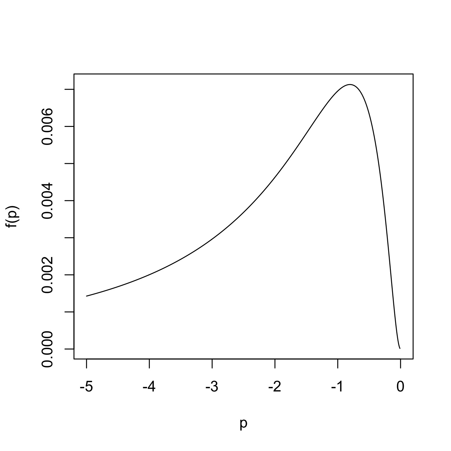
3.2. Optimal in the Hall class
We now make a further assumption on the regularly varying class, in order to get an explicit form of . Concretely, we assume the Hall class (Hall, 1982), which satisfies the property
| (20) |
An immediate consequence then is the explicit expression
Hence,
| (21) |
Recall that the classical Hill estimator for this class has AMSE given by
which is minimized for
| (22) |
see e.g. (Beirlant et al., 2004, p.125)). In a similar way, the minimizer of (21) is simply
| (23) |
Hence from (22) and (3.2) we obtain a simple expression of the optimal threshold of the Hill estimator in terms of :
| (24) |
3.3. Interpretation of as a weighted Hill estimator
Observe that, for fixed ,
| (25) |
with
so that one can interpret the estimator as a modification of the classical Hill estimator that uses different weights for different order statistics. It is not hard to see that asymptotically the correction factors behave like
| (26) |
Figure 7(left) highlights the accuracy of this approximation for across different values of , and also illustrates the fact that the largest data point receives a weight of almost 2 in this case, whereas on from the 20th-largest observation the weight is lower than for the classical Hill estimator, and the weight diminishes for smaller data points. Note that, as increases, the weight of the largest observation grows above any bound, but extremely slowly, namely
Figure 7(right) illustrates that even for a value as large as , is still below 2.4.
4. A ratio statistic
Once a has been selected, it is important to be able to statistically assess whether the remaining upper tail differs significantly from the one of a pure Pareto. In order to recognize whether a Pareto tail has been achieved or not, we have seen that flatness of the lower-trimmed Hill estimator is desirable. Inspired by the T-statistic introduced in Bhattacharya et al., 2019, we introduce the ratio statistics
quantities which we expect to be close to one. Although these statistics do not have the property of being i.i.d. and hence test sizes have to be calibrated using Monte Carlo simulation, an advantage which carries over to the present setting is that they do not depend on . Indeed, defining , we have
by the order statistics property of the Poisson process, where, , and , , is an i.i.d. sequence of independent unit-rate exponential random variables. This invariance with respect to the parameter permits to assess the goodness of selection of a threshold as follows:
- (1)
Simulate the statistics times, and call them
- (2)
For fixed , find the empirical and quantiles corresponding to each of the samples,
and call them .
- (3)
Count the proportion of the trajectories
which for some fall outside of their confidence interval . Call this proportion .
- (4)
The proportion is the global level of the test, and the algorithm stops when it is close enough to a pre-specified level (typically ). If is larger (smaller) than the pre-specified level, go to Step (2) and decrease (increase) .
- (5)
Plot the , , from the data, together with the last set of quantiles . It is also a good idea, for visualization, to plot the standardized version
which for a pure Pareto tail is expected by construction to lie (as a trajectory) between and in of the cases. Here, we have used the notation .
Example 4.1.
For the Burr sample of Figure 4, we compare taking and in the plots of Figure 8. The first number, is precisely the one that minimizes the expected empirical variance, according to the parameters of the Burr sample and to formula (3.2), with chosen to be . The number of Monte Carlo simulations was in each case , and the significance level is . Observe how the fit is good for , but is outside the bands for .
Remark 4.1.
This approach can only be considered as a selection procedure itself if the corresponding sequential testing is adjusted to have the correct size. In other words, if the above algorithm is used multiple times to choose , the rejection probability will exceed the desired level. An alternative is to take sequential values of into the algorithm, which makes the routine highly computationally intensive. Hence, we presently recommend it solely as a goodness of selection evaluation.

5. Simulations
We perform a simulation study based on three different and common distributions which belong to the Hall class (20). We consider simulating times from the following three distributions, with four sub-cases for each distribution, for varying sample size and parameters:
- •
The Burr distribution, with tail given by
which implies by Taylor expansion that
We consider for the two sets of parameters , , ; and , , .
- •
The Fréchet distribution with tail
which implies
We consider for the two parameters .
- •
The Generalized Pareto Distribution (GPD) distribution, with tail given by
which implies
We consider for the two sets of parameters , ; and , .
- •
The Student-t distribution with degrees of freedom. The tail is given in terms of hypergeometric and Gamma functions. Since this distribution is symmetric around zero, we take the absolute values of the data, which preserves the tail behaviour. We have that
We consider, for , the two sets of parameters .
For each sample we evaluate the Hill estimator
and the averaged trimmed estimator
at three particular choices of . Note that these threshold choices are designed for the Hill estimator, but will turn out sensible for the latter estimator as well.
- (i)
We use the popular procedure of Guillou and Hall, 2001 as a benchmark for finding the optimal choice of , and denote the resulting tail estimators by , . Such a threshold selection procedure has been subject to comparisons (both in Guillou and Hall, 2001 itself and in Beirlant et al., 2002) to other alternatives like Danielsson et al., 2001 and Drees and Kaufmann, 1998. We also refer to Schneider et al., 2019 for a recent paper which was developed independently around the same time as the present article.
- (ii)
An estimator of from (22) is obtained as follows. Motivated by (21), we compute as the minimizer of the empirical variance (the search beginning at 1/5 of the sample size, to avoid degeneracies) of the trimmed Hill estimator, as a function of , and using (24) to set
Observe that while we still have to input , here prior knowledge of is no longer needed. We choose as the canonical choice.
- (iii)
As in (ii), but using the true parameter of , in order to quantify how the removal of a potential misspecification of by the canonical choice affects the estimators. The results obtained when using an estimator of , such as given by Fraga Alves et al., 2003, rather than fixing it at a fixed value, indicated that the additional variability by including an additional estimator does not lead to further improvements at smaller sample sizes. This confirms the observations made for instance in Drees and Kaufmann, 1998 and Beirlant et al., 2002.
We then plot the bias, variance and MSE of each resulting estimator as a function of .
The results are given in Figures 9, 10 for the Burr case; Figures 11, 12 for the Fréchet case; Figures 13, 14 for the GPD case; and Figures 15, 16 for the Student-t case. We observe that the behaviour is very similar for the four families (which is not uncommon in this context, cf. (Beirlant et al., 2002, p.178)).
For the Hill estimator, we notice that our method fares well against the benchmark. The misspecification of the second order parameter does not play a substantial role, except perhaps for the most biased case of the Student-t distribution with degrees of freedom. The same behaviour is observed within the three -estimators. When comparing Hill against -estimators, the latter improve the bias and MSE for nearly all , and in most cases also the variance (except for very heavy tails () and small values of ).
Remarkably, the estimator , where the canonical is used, is highly competitive against the Hill estimator, especially so for . This is not a contradiction, since the optimality of the Hill estimator refers to choices for within the class of , whereas the estimators span a different class (visible in the weighting interpretation of Section 3.3), and when is optimized w.r.t. AMSE in that class, even better performance can be feasible, which, however, is not the subject of the present paper.
6. Insurance data
Let us now consider a real-life insurance data set consisting of motor third party liability (MTPL) insurance claims from the period 1995-2010 that was studied intensively in Albrecher et al., 2017 (where it is referred to as ”Company A”). These data are right-censored, and were also analyzed recently combining survival analysis techniques and expert information in Bladt et al., 2019. Here, we focus only on the ultimates, see Figure 17, which are the actual final claim sizes for the settled claims and an expert prediction of the total payment until closure for all claims that are still open.


In Figure 18 we depict the lower-trimmed Hill plots and the usual Hill plot, together with the empirical variance. We have also included , which follows somewhat closely the trajectory of the usual Hill plot, and the mean-of-order bias-reduced estimator. As a preliminary observation, notice that the -area at which visually the Hill plot and its bias-reduced version start to differ is roughly the same as where the lower trimmed Hill trajectories start flattening out, which serves as a good sanity check. As in the simulation studies in Section 5, in order to avoid degeneracies, we only look at candidates for the minimizer to the right of , which corresponds to in this case. The minimum empirical variance is then obtained for . Using the canonical choice , we have that . Note that for the same choice , using the prior eyeballed estimate , and based on the Burr-like Hill plot, we can deduce that , and then . We thus get by (22) the ad-hoc sample fraction (which might be considered the classical choice of the threshold in this case). Notice, however, that the latter estimate is only available heuristically, since one needs a first estimate of to estimate itself, and also to make distributional assumptions on the data. We include this estimate here simply as a naive solution that requires no further statistical procedures beyond looking at the Hill plot.


The corresponding estimates of are given by
The simulation studies of Section 5 may suggest the third of the above numbers to be the most reliable estimate, since there is no way of quantifying the eyeball-aided procedure involving . However, the confidence interval for the first estimate is , suggesting that for a one-sample analysis, it is difficult to make a definitive statement on the statistical superiority of any of the four estimates. Further, the ratio statistic test in Figure 19 suggests that for both thresholds the sample is Pareto in the tail (with only a slight issue for the two largest observations). The takeaway is that, roughly speaking, we are able to reconfirm in an automated statistical way what can be deduced by looking at a Hill plot (together with its bias-reduced variants) and guessing the distribution of the sample.
In (Albrecher et al., 2017, p.99), a splicing point was suggested for this data set at around , based on expert opinion. A semi-automated option using our method for detecting this splicing point would be to
replace the left limit by a very small number (in this case is chosen after visual insection of the erratic nature of the empirical variance for the first three), and then to apply our method, which leads to the detection of the minimum variance at (which is clearly visible in Figure 18). Under the assumption this then leads to as a suggested splicing point. We would like to point out that the identification of the splicing point matters in insurance practice, since the different resulting distributional assumptions on either side then have an effect on the location of extreme quantiles and risk management in general, including the capital requirements for solvency purposes. The possibly natural existence of splicing points can also be argued from a causal perspective, as different degrees of inspection scrutiny may be applied below and above certain claim levels.
As a side remark, in the present data set the ultimates for the highest claims have a certain degree of intrinsic uncertainty (as they are just estimates of the final closed claim size), and a more systematic way to approach this particular situation would be to combine the trimming of the Hill estimator from below and above, but the latter is not the focus of the present paper.

7. Conclusion
In this paper, we showed that trimming the Hill estimator from the left can lead to favorable properties in connection with the expected empirical variance of the tail index estimators in extreme value statistics. For the Hall class, we established asymptotic results on the behavior of this expected empirical variance, which allows to develop a guideline for the choice of the optimal threshold in the tail index estimation problem. It turns out that there is an intrinsic link between this optimal threshold and the classical optimal threshold for the Hill estimator. Since in the trimming context the identification of the optimal threshold is much more insensitive on the tail characteristics (it only depends on the -parameter in the Hall class, not on nor on the tail index ), this link allows to circumvent the classical problem in threshold selection for the Hill estimator. As a by-product, by suitable averaging we develop a novel tail index estimator which assigns a non-uniform weight to each observation in a natural way, relies on fewer assumptions on the tail characteristics, is simple to implement and outperforms the classical Hill estimator in most cases. The latter is illustrated in simulation studies. In addition, the technique is applied to a real-life insurance data set that was previously studied by other techniques. Note also that the proposed selection principle for based on the variance of the lower-trimmed Hill plots can be applied to any estimator of for which the asymptotic mean squared error can be written as with and only depending on . We conclude by noting that the approach taken in this paper is in principle also applicable for the potential improvement of tail index estimators other than the Hill estimator. Further possible directions of future research include the combination of left trimming with right trimming in situations with possible outliers, as well as the consideration of possibly censored data.
Acknowledgement. M.B. and H.A. acknowledge financial support from the Swiss National Science Foundation Project 200021_191984.
References
- Albrecher et al., (2017) Albrecher, H., Beirlant, J., and Teugels, J. L. (2017). Reinsurance: Actuarial and Statistical Aspects. John Wiley & Sons, Chichester.
- Bader et al., (2018) Bader, B., Yan, J., and Zhang, X. (2018). Automated threshold selection for extreme value analysis via ordered goodness-of-fit tests with adjustment for false recovery rate. Ann. Appl. Statistics, 12:310–329.
- Beirlant et al., (2011) Beirlant, J., Boniphace, E., and Dierckx, G. (2011). Generalized sum plots. REVSTAT-Statistical Journal, 9(2):181–198.
- Beirlant et al., (2002) Beirlant, J., Dierckx, G., Guillou, A., and Stǎricǎ, C. (2002). On exponential representations of log-spacings of extreme order statistics. Extremes, 5(2):157–180.
- Beirlant et al., (2004) Beirlant, J., Goegebeur, Y., Segers, J., and Teugels, J. L. (2004). Statistics of extremes: theory and applications. John Wiley & Sons, Chichester.
- Beirlant et al., (1996) Beirlant, J., Vynckier, P., and Teugels, J. L. (1996). Tail index estimation, pareto quantile plots regression diagnostics. Journal of the American Statistical Association, 91(436):1659–1667.
- Bhattacharya et al., (2019) Bhattacharya, S., Kallitsis, M., and Stoev, S. (2019). Data-adaptive trimming of the Hill estimator and detection of outliers in the extremes of heavy-tailed data. Electronic Journal of Statistics, 13:1872–1925.
- Bladt et al., (2019) Bladt, M., Albrecher, H., and Beirlant, J. (2019). Combined tail estimation using censored data and expert information. Scandinavian Actuarial Journal, DOI:10.1080/03461238.2019.1694974.
- Buitendag et al., (2019) Buitendag, S., Beirlant, J., and de Wet, T. (2019). Ridge regression estimators for the extreme value index. Extremes, 22:271–292.
- Csörgő et al., (1985) Csörgő, S., Deheuvels, P., and Mason, D. (1985). Kernel estimates of the tail index of a distribution. Ann. Statist., 13(3):1050–1077.
- Danielsson et al., (2001) Danielsson, J., de Haan, L., Peng, L., and de Vries, C. G. (2001). Using a bootstrap method to choose the sample fraction in tail index estimation. Journal of Multivariate analysis, 76(2):226–248.
- de Haan and Ferreira, (2007) de Haan, L. and Ferreira, A. (2007). Extreme value theory: an introduction. Springer Science & Business Media.
- De Sousa and Michailidis, (2004) De Sousa, B. and Michailidis, G. (2004). A diagnostic plot for estimating the tail index of a distribution. Journal of Computational and Graphical Statistics, 13(4):974–995.
- Draisma et al., (1999) Draisma, G., de Haan, L., Peng, L., and Pereira, T. T. (1999). A bootstrap-based method to achieve optimality in estimating the extreme-value index. Extremes, 2(4):367–404.
- Drees et al., (2000) Drees, H., de Haan, L., and Resnick, S. (2000). How to make a Hill plot. The Annals of Statistics, 28(1):254–274.
- Drees et al., (2020) Drees, H., Janßen, A., Resnick, S. I., and Wang, T. (2020). On a minimum distance procedure for threshold selection in tail analysis. SIAM Journal on Mathematics of Data Science, 2(1):75–102.
- Drees and Kaufmann, (1998) Drees, H. and Kaufmann, E. (1998). Selecting the optimal sample fraction in univariate extreme value estimation. Stochastic Processes and their Applications, 75(2):149–172.
- Embrechts et al., (2013) Embrechts, P., Klüppelberg, C., and Mikosch, T. (2013). Modelling extremal events: for insurance and finance, volume 33. Springer Science & Business Media, second edition.
- Fraga Alves et al., (2003) Fraga Alves, M., Gomes, M., and de Haan, L. (2003). A new class of semi-parametric estimators of the second order parameter. Portugaliae Mathematica, 60:193–213.
- Gomes et al., (2016) Gomes, M. I., Brilhante, M. F., and Pestana, D. (2016). New reduced-bias estimators of a positive extreme value index. Communications in Statistics - Simulation and Computation, 45(3):833–862.
- Gomes et al., (2008) Gomes, M. I., de Haan, L., and Rodrigues, L. H. (2008). Tail index estimation for heavy-tailed models: accommodation of bias in weighted log-excesses. Journal of the Royal Statistical Society: Series B (Statistical Methodology), 70(1):31–52.
- Gomes and Guillou, (2015) Gomes, M. I. and Guillou, A. (2015). Extreme value theory and statistics of univariate extremes: a review. International Statistical Review, 83(2):263–292.
- Gomes and Oliveira, (2001) Gomes, M. I. and Oliveira, O. (2001). The bootstrap methodology in statistics of extremes—choice of the optimal sample fraction. Extremes, 4(4):331–358.
- Gomes and Pestana, (2007) Gomes, M. I. and Pestana, D. (2007). A sturdy reduced-bias extreme quantile (var) estimator. Journal of the American Statistical Association, 102(477):280–292.
- Guillou and Hall, (2001) Guillou, A. and Hall, P. (2001). A diagnostic for selecting the threshold in extreme value analysis. Journal of the Royal Statistical Society: Series B (Statistical Methodology), 63(2):293–305.
- Hall, (1982) Hall, P. (1982). On some simple estimates of an exponent of regular variation. J. Roy. Statist. Soc. Ser. B, 44(1):37–42.
- Hall, (1990) Hall, P. (1990). Using the bootstrap to estimate mean squared error and select smoothing parameter in nonparametric problems. Journal of multivariate analysis, 32(2):177–203.
- Hall et al., (1985) Hall, P., Welsh, A., et al. (1985). Adaptive estimates of parameters of regular variation. The Annals of Statistics, 13(1):331–341.
- Hill, (1975) Hill, B. M. (1975). A simple general approach to inference about the tail of a distribution. The Annals of Statistics, 3:1163–1174.
- Papastathopoulos and Tawn, (2013) Papastathopoulos, I. and Tawn, J. (2013). Extended generalised pareto models for tail estimation. Journal of Statistical Planning and Inference, 143(1):131–143.
- Schneider et al., (2019) Schneider, L., Krajina, A., and Krivobokova, T. (2019). Threshold selection in univariate extreme value analysis. Arxiv:1903.02517v1.
8. Proofs
Proof of Proposition 2.1. Set . By the Rényi representation (6),
Plugging in () gives
which corresponds to the usual variance of the Hill estimator and gives the first identity. In the general case,
But implies , such that
so
Thus
which gives the second identity.
∎
Proof of Theorem 3.1. We first note that
where are the order statistics of a standard Pareto sample (the case). Then, from the second order condition (14) we obtain that for and , as ,
But by the Rényi representation (6) of exponential order statistics, the first term is distributed as
where are i.i.d. standard exponential random variables. For the second term, by convergence to uniform random variables and a Riemann integral approximation, we get
and since is a uniform order statistic, we further get that
Putting the three pieces together then establishes (15). ∎
Proof of Theorem 3.2. With the shortened notation, we write
| (27) |
and by exchange of the order of summation, we can write
Again, by Riemann integration we have that
and
Similarly,
| (28) |
Putting the pieces together then indeed yields (18).
∎
Proof of Theorem 3.3. Let us first decompose each summand by writing
and subsequently consider each term separately. From (27) we have that
On the other hand, (18) gives
The third term can be analyzed using both (18) and (27) as follows,
where .
We now proceed to add the summands of the expected variance. To this end, some preparatory calculations will be helpful. By (17) and Riemann approximation we have
By virtue of (8),
from which we deduce that as ,
where is given by (19).
Observe that for the terms arising from the expected covariance term
Next,
and
Finally, for the mean squared error term of we find
Altogether we hence obtain
with
∎