A Spatial Bayesian Semiparametric Mixture Model for Positive Definite Matrices with Applications to Diffusion Tensor Imaging
Abstract
Diffusion tensor imaging (DTI) is a popular magnetic resonance imaging technique used to characterize microstructural changes in the brain. DTI studies quantify the diffusion of water molecules in a voxel using an estimated symmetric positive definite diffusion tensor matrix. Statistical analysis of DTI data is challenging because the data are positive definite matrices. Matrix-variate information is often summarized by a univariate quantity, such as the fractional anisotropy (FA), leading to a loss of information. Furthermore, DTI analyses often ignore the spatial association of neighboring voxels, which can lead to imprecise estimates. Although the spatial modeling literature is abundant, modeling spatially dependent positive definite matrices is challenging. To mitigate these issues, we propose a matrix-variate Bayesian semiparametric mixture model, where the positive definite matrices are distributed as a mixture of inverse Wishart distributions with the spatial dependence captured by a Markov model for the mixture component labels. Conjugacy and the double Metropolis-Hastings algorithm result in fast and elegant Bayesian computing. Our simulation study shows that the proposed method is more powerful than non-spatial methods. We also apply the proposed method to investigate the effect of cocaine use on brain structure. The contribution of our work is to provide a novel statistical inference tool for DTI analysis by extending spatial statistics to matrix-variate data.
Keywords: Bayesian semiparametric, Diffusion tensor imaging, Inverse Wishart distribution, Matrix-variate, Positive definite matrix, Spatial statistics
1 Introduction
Measurement of signal attenuation from water diffusion, often considered one of the most important magnetic resonance contrast mechanisms (Alexander et al. 2007), is usually achieved via diffusion tensor imaging (DTI) that maps and characterizes the 3-D diffusion of water molecules as a function of the spatial location (Basser et al. 1994). The diffusion process in the brain reflects interactions with many obstacles, such as fibers, thereby revealing microscopic details about the underlying tissue architecture. Unlike ordinary images where scalars are summarized for each voxel, a distinguishing feature of DTI is each voxel is associated with a symmetric positive definite matrices which can be interpreted as the covariance matrix of a 3-D Gaussian distribution modeling the local Brownian motion of the water molecules (Schwartzman et al. 2008). These positive definite matrices are also called the diffusion tensors (DTs). One important clinical application of the DTI is to detect regions of local differences in the brain between two groups (i.e., normal versus disease), revealing anatomical structural differences (Lo et al. 2010). For example, the motivating data for this paper comes from a clinical DTI study (Ma et al. 2017), where the scientific objective is to detect regions of differences between cocaine users and non-cocaine users.
Statistical analysis of DTI data is challenging due to the difficulty of modeling matrix-variate responses. One option is to project the DTs into fractional anisotropy (FA), a scalar describing the degrees of anisotropy of a diffusion process. However, some information is lost because different positive definite matrices may produce the same FA (Ennis and Kindlmann 2006). Matrix-variate methods potentially avoid information loss. There are relatively few matrix-variate methods available to analyze DTI data, and they can be broadly classified into the (inverse) Wishart matrix methods (Dryden et al. 2009) and the random ellipsoid models (Schwartzman et al. 2008; Lee and Schwartzman 2017). However, these voxel-level models ignore information from neighboring voxels that may have similar neuronal activity (see Figure 1), despite recommendations of incorporating this non-negligible spatial association to achieve efficient and valid inference (Spence et al. 2007) as well as studies revealing that the disease status at proximally-located/neighboring voxels can be similar (Wu et al. 2013; Xue et al. 2018, see). This motivates us to develop an improved spatial statistical model which (a) utilizes full matrix information, (b) captures spatial dependence, and (c) can be implemented via fast and elegant computing.

The spatial neuroimaging toolbox for univariate responses is considerably rich: Woolrich et al. 2004b proposed a fully Bayesian model for spatiotemporal imaging data; Kang et al. 2011 implemented spatial point processes for meta-analysis of imaging data; To select essential biological features, Musgrove et al. 2016 introduced spatial Bayesian variable selection for neuroimaging data; Recently, Reich et al. 2018 proposed spectral methods for ADNI data to provide computational benefits. All of these studies demonstrated an improvement in the precision of estimates by properly accounting for spatial dependence.
In this vein, the Potts model, a generalization of the Ising model in statistical mechanics, has also been successfully applied to imaging (Johnson et al. 2013; Li et al. 2018). A desirable property of the Potts model is that it avoids smoothing over abrupt changes in the image intensity (Johnson et al. 2013), and this makes it more attractive than available Gaussian kernel methods. To this end, we assume the positive definite DTs follow a mixture of inverse Wishart distributions, with the mixture component labels modeled via a (spatial) Potts model, representing a discrete Markov random field. This semiparametric mixture specification refers to a class of flexible mixture distributions with a finite number of components (Lindsay and Lesperance 1995).
Besides spatial modeling, another important topic in neuroimaging is detecting regions of differences between two groups. Previous attempts at identifying regions of differences between two groups were formulated through voxel-wise hypothesis testing (Schwartzman et al. 2008; Lee and Schwartzman 2017). An alternative option is to construct multilevel hierarchical modeling accounting both subjective-level and group-level variation and use the group-level parameters for voxel-wise hypothesis testing (Woolrich et al. 2004a; Liu et al. 2014). In this paper, we use the latter approach via extending the latent classic Potts model into a hierarchical two-way framework, allowing hypothesis testing via group-level parameters and inter-subject variability simultaneously.
Our proposal is implemented using the Bayesian approach, accounting for the uncertainty of model parameters in all levels of the hierarchy. However, the Bayesian approach is often problematic in neuroimaging because of its heavy computational burden (Cohen et al. 2017). Although the associated Markov chain Monte Carlo (MCMC) algorithm is mostly composed of computationally tractable Gibbs steps that can be paralleled, a major drawback of the Potts model is the intractable normalizing constant, creating a bottleneck for hyperparameter updates. In this paper, it is resolved via the double Metropolis-Hastings algorithm (Liang 2010) recommended by Park and Haran 2018.
To the best of our knowledge, this is the first work on exploring spatial associations in modeling positive definite matrix-variate data under a Bayesian semiparametric framework, with applications to DTI. In the rest of the paper, we first introduce the single-subject and multi-subject model, and the group hypothesis testing framework in Section 2. Relevant MCMC computational details appear in Section 3. To demonstrate the improvement in performance compared to plausible alternatives, we perform simulation studies in Section 4. In Section 5, we present the application to the motivating cocaine data set. Finally, Section 6 concludes with a discussion.
2 Model
In this section, we introduce the spatial Bayesian semiparametric mixture model for positive definite matrices. We introduce the single-subject model first in Section 2.1 and then extend to the multi-subject model in Section 2.2.
2.1 Single-Subject Model
Let be the DT at voxel . To ensure is symmetric and positive definite, it is usually parameterized as a (inverse) Wishart matrix (Dryden et al. 2009) or a Gaussian symmetric matrix-variate distribution (Schwartzman et al. 2008). In this paper, we assume that follows an inverse Wishart distribution as
| (1) |
where is the inverse Wishart distribution parameterized (Appendix A) to have mean and degrees of freedom , and the DTs are independently distributed across given the mean matrices and the degrees of freedom . The mean matrices are modeled as a finite mixture of Wishart distributions, denoted as where is the latent cluster label. The prior of is where is the Wishart distribution parameterized (Appendix A) to have mean and degrees of freedom .
Spatial dependence of the DTs is achieved through the dependence of the mean matrices . We induce spatial dependence via the latent cluster labels that follow a weighted Potts model, specified via the full conditional distributions:
| (2) |
where is the full set excluding , is a set of indices of the neighboring voxels of , and if event is true and otherwise. Given but marginal over , the distribution of is the mixture of inverse Wishart distributions:
where is the inverse Wishart density function of with the mean matrix and the degrees of freedom . Therefore, this semiparametric mixture model spans a rich class of density functions.
Via the Potts model, an image can be considered as a network whose nodes are the voxels. In this network, every voxel is connected to its neighboring voxels. The full conditional distribution of depends only on the voxels in the neighboring set and therefore the process is Markovian. Since the spatial parameter is the coefficient of the neighboring term , the spatial parameter controls the dependence on the neighboring voxels.
Unlike the classic Potts model (Wu 1982), the terms are added as offset terms controlling the overall mass on each cluster. We set so the parameter is the concentration parameter controlling the homogeneity of the latent cluster labels. It is problematic to pre-specify the number of components in a mixture model (McCullagh et al. 2008) but the offset terms provide more weight on the key components and fewer weights on the trivial components. We fit the model by setting to be an upper bound on the number of active clusters and allow the data to determine the number of active clusters via estimation of : if , there are several active clusters; if is large, there are a few active clusters. As a result, the model is less sensitive to the number of components when the offset term is included. This claim is verified in the simulation studies (Section 4) and the real data application (Section 5), where we find similar results for different .
Quantifying spatial dependence is a vital issue in spatial statistics and neuroimaging. Since this model is for matrix-variate data, we use the expected squared Frobenius norm to measure dependence. The dependence between matrices and can be summarized as . The norm increases as dependence decreases. If and are , the expected squared Frobenius norm is the classic variogram (Cressie 1992) of spatial statistics. In this regard, the expected squared Frobenius norm can be treated as the variogram for matrix-variate data and useful in measuring spatial dependence. In the rest of the paper, we simply call the expected squared Frobenius norm the variogram.
For the Potts model described above, the variogram is
where is the marginal (over all other cluster labels ) probability of , and is a measure of the variability in and variability of across . Therefore, the multivariate spatial dependence structure is separable (Cressie 1992) in that the dependence is the product of a non-spatial term that controls cross dependence and a spatial term that controls spatial dependence.
We give the expression of in Appendix B. When and , the non-spatial term has an expression that is where and . Therefore, in this special case, the cross dependence decreases if or is larger (See Figure 2).
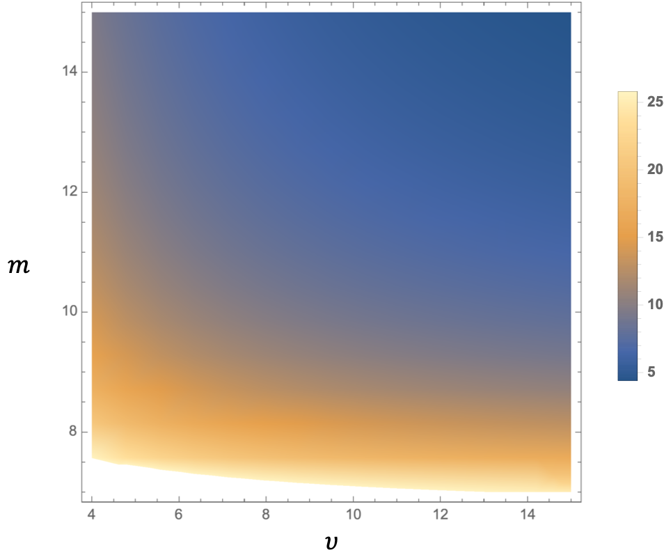
The spatial term is intractable and so we use a Monte Carlo approximation to study the function. In Figure 3(a), the function is computed under the scenario that the image is a 1-D grid with and . The spatial term increases with distance and larger spatial parameter leads to the stronger spatial dependence. We also compute the function value with different in Figure 3(b). We have , where relevant result can be found in studies of extreme value analysis (Reich and Shaby 2018, see). Increasing leads to smaller spatial dependence. Hence, we fix to be large to eliminate long-range dependence (i.e., for large ) and estimate to capture local dependence.
For a more intuitive understanding of this model, we also simulate the DTs and visualize the DTs as ellipsoids in a grid. In these simulations, we use , , and . In Figure 4(a), the DTs within the same latent cluster label are similar to each other, indicating that spatial dependence of the DTs can be achieved by the latent cluster labels following the Potts model. In Figure 4(b), larger spatial parameter leads to a realization with more dependence on their neighbors. Figure 4 also illustrates that the Potts model allows sharp breaks, which is desirable if neighboring voxels are in different tracts.


2.2 Muti-Subject Model
Motivated by the cocaine users data set (Ma et al. 2017) that includes 11 cocaine users and 11 non-cocaine users, we extend the single-subject model to the multi-subject setting. The clinical objective is to analyze the brain’s physical structure for differences between the two groups. The objective can be statistically formulated as finding regions in the brain where the distribution of the DTs across the subjects is different between cocaine users and non-cocaine users.
Let be the DT and be the cluster label for voxel and subject . By extending to , the subject-level cluster labels not only model intra-subject spatial dependence but also allow inter-subject variability. As in the single-subject model, the DTs are conditionally independent given the random matrices following a finite mixture model:
| (3) |
However, the latent Potts model is generalized to account for multiple subjects. We define as the binary group indicator of subject . In the motivating data, cocaine users have and non-cocaine users have . To model intra-subject spatial dependence within a group, we extend the latent cluster process by introducing the group-level cluster labels for group and voxel . Both and are also spatially dependent with full conditional distributions
| (4) | ||||
where is the set on excluding , is the set excluding , is the set on , and is the set on . The joint probability mass function (PMF) of is given in Appendix C. Since the conditional densities in (4) satisfy the conditions of the Hammersley-Clifford Theorem (Clifford 1990), the existence of joint distribution of is guaranteed (Appendix C).
A graphical representation of this latent Potts model is provided in Figure 5. Cluster labels and can be understood as the spatial pattern of subject and the general spatial pattern of subjects in group , respectively. In comparison to the single-subject model, the group-clustering parameter is introduced for modeling multiple subjects. If , is independently distributed over subjects; otherwise, the subject-level cluster label depends on the group-level cluster label , leading to the smaller inter-subject variability of spatial dependence pattern within one group.

To further understand the role of and , we inspect the density of conditioned on and marginal over all other labels (Appendix D). The conditional density of given and is the mixture of inverse Wishart distributions proportional to
| (5) |
where the term is the proportional weight of cluster . Therefore, elevates the mass on mixture component at voxel for all subjects with . Assuming , the conditional density (5) depends on if and only if .
The clinical objective is to find regions of differences between two groups, which can be formulated into finding voxels for which the distribution of is different for or . As shown in the conditional density (5), the test can be simplified to the test that
| (6) | ||||
Bayesian inference provides estimates of the posterior probabilities of the hypotheses, which is further discussed in Section 3.
We investigate spatial dependence as in the single-subject model. To measure spatial dependence within and across subjects, we propose the variogram
| (7) |
with for individual variogram and for inter-subject variogram, respectively. For inter-subject variogram, we also compare the within-group variogram for subjects with and between-group variogram for subjects with . Both individual variogram and inter-subject variogram are also separable (Cressie 1992). is the non-spatial term which has been discussed in Section 2.1. The spatial term is the marginal probability of .
In Figure 6(a), the function is computed using a Monte Carlo approximation under the scenario that the image is a 1-D grid with and . The spatial parameter largely controls the within-subject dependence. In Figure 6(b) plotting , larger leads to more dependence in the within-group variogram. Therefore, controls the dependence of subjects within one group. Since and are assumed to be independent, the spatial term is a constant in between-group variogram (Figure 6(c)).


3 Computation
We use MCMC to fit the model described in Section 2 (Appendix E). The codes are written in hybrid R and C++ codes. The final model is
| (8) | ||||
which is referred to as the Potts Model in the rest of the paper. Using the moment method (Robert 2007)[Section 3.2.4], we set as the sample mean of all observed DTs. The priori information brought by has a little impact if the number of observations is large. We put uniform prior for the degrees of freedom and on . Following Liang 2010, we put a uniform prior for on , denoted as . Below we describe the updating rule for each parameter.
The MCMC algorithm is a combination of Gibbs and Metropolis-Hastings steps. The latent mean matrices and cluster labels are updated via Gibbs steps. Their full conditional distributions are
- •
- •
- •
where . In addition, and can be updated in parallel over and , respectively. Since the uniform prior is not conjugate, we have to sample and via Metropolis-Hastings sampling with log-normal random walk as proposal distribution.
To select regions of differences via Bayesian hypothesis testing, we reject the null hypothesis in (6) if . The posterior probabilities can be estimated through MCMC samples that or .
Updating the Potts hyperparameters , , and is problematic because the normalizing constant in the joint distribution function of the cluster labels is intractable (see the joint PMF in Appendix C). A simple approach is to estimate the parameters outside of MCMC. The plug-in values can be obtained from cross-validation (Goldsmith et al. 2014, i.e.,), pseudo-likelihood comparison (Zhao et al. 2014; Lan et al. 2016, i.e.,), or by comparing empirical and model-based variograms (i.e., Figure 7 and 9). However, these methods fail to account for uncertainty about these imputed parameters and so we update them using the double Metropolis-Hastings algorithm (Liang 2010).
Park and Haran 2018 review several Monte Carlo methods for models with intractable normalizing constants and recommend the double Metropolis-Hastings algorithm proposed by Liang 2010 because of its ease of implementation and computational efficiency. Li et al. 2018 combine the double Metropolis–Hastings algorithm with usual Bayesian tools for implementing the Potts model. The double Metropolis-Hastings update for begins with a candidate drawn from where is the current value and is a log-normal random walk transitional probability centered at . Given the candidate , we draw labels and using Gibbs sampling for each and , respectively. The candidate is accepted with the probability where where is the likelihood of conditioned on . and are current values. Due to the concern that the double Metropolis-Hastings algorithm is not an exact sampling (Liang 2010; Park and Haran 2018), the MCMC convergence of in the simulation studies (Section 4) and the real data analysis (Section 5) are monitored by Heidelberger and Welch’s convergence diagnostic (Heidelberger and Welch 1981).
4 Simulation
In this section, we illustrate the performance of our method using two simulation studies under different scenarios for synthetic data. We compare our method to the non-spatial DTI inference method the Gaussian symmetric matrix model (Schwartzman et al. 2008) referred to as the Random Ellipsoid Model. The Random Ellipsoid Model is a non-spatial matrix-variate method and assumes that follows a Gaussian symmetric random matrix distribution with the probability density function (PDF) as , where is the DT’s population mean at voxel of group and is the nuisance parameter. The Random Ellipsoid Model selects regions of differences via testing , where the test statistics are constructed by maximum likelihood estimations. the Potts Model has MCMC samples with discarded as burn-in. Methods are evaluated in terms of true positive rate (TPR), false positive rate (FPR), false discovery rate (FDR), and typical computation time.
We first investigate the performance of our method when the data are generated from a mixture model. We use a grid with spacing 1 between adjacent grid points as an image. Each simulated data set consists of 5 subjects in the control group () and 5 subjects in the treatment group (). For the control group (), we equally partition the graph into 4 parts by rectangular regions so that , ordered by right-to-left. Thus each region is a region. The treatment group has the same partition as the control group, except a region at the middle of the second region where . This simulates the brain with a small region of difference between the two groups. For each simulation, is generated based on the model
Given the simulated , the data are generated based on the model .
Our model with is compared to the Random Ellipsoid Model. The results averaged over 50 data sets are summarized in Table 1(a). Our model has significantly improved performance in terms of the TPR, FPR, FDR in comparison to the Random Ellipsoid Model. The small number of subjects might be one of the causes that the alternative produces low TPR. Schwartzman et al. 2008 discusses that the accuracy of maximum likelihood estimates of the Random Ellipsoid Model is dependent on the number of subjects. Since the choice of does not affect selection accuracy, the simulation results also support the claim that the model can be less sensitive to the number of clusters if is larger than the true clusters.
To determine robustness to model misspecification, we also simulate data from the spatial Cholesky process described as follows: The DT matrix for subject at voxel is determined by six independent spatial Gaussian processes (). These spatial Gaussian processes are arranged in the lower triangular matrix with . The responses are then constructed as , thereby introducing spatial dependence and guaranteeing positive definite of responses. We again use a grid with spacing 1 between adjacent grid points as an image. There are 10 subjects in the control group and 10 subjects in the treatment group. The six spatial Gaussian processes are simulated with variance and exponential correlation function with range parameter . The mean of the six Gaussian processes are all except for treatment subjects’ region in the center of the image where has mean for and for . This simulates the brain with a small region of difference between the two groups. We compare our model with to the Random Ellipsoid Model. The results averaged over 50 simulations are summarized in Table 1(b). The results demonstrate that our model maintains good performance, indicating the Potts Model is robust to this form of misspecification. In addition, under the spatial dependence assumption, the spatial models produce an overall better performance than the non-spatial model.
A problematic issue to the use of Bayesian methods in neuroimaging data is their heavy computational burden. In both simulations, the Potts Model has a computational speed within a few hours. The Random Ellipsoid Model avoids the expensive MCMC, but since the performance of the Random Ellipsoid Model is too conservative, the Potts Model is a reasonable trade-off.
| Method | Potts | Random Ellipsoid | ||
|---|---|---|---|---|
| K=10 | K=50 | K=100 | ||
| TPR | 0.99 | 0.97 | 0.98 | 0.29 |
| FPR | 0.013 | 0.010 | 0.009 | 0.00 |
| FDR | 0.025 | 0.025 | 0.024 | 0.002 |
| Time (hours) | 0.5 | 0.8 | 1.0 | 0.01 |
| Method | Potts | Random Ellipsoid | |||
|---|---|---|---|---|---|
| K=10 | K=50 | K=100 | |||
| TPR | 0.79 | 0.80 | 0.77 | 0.50 | |
| FPR | 0.01 | 0.01 | 0.01 | 0.00 | |
| FDR | 0.03 | 0.03 | 0.02 | 0.03 | |
| Time (hours) | 1.0 | 1.5 | 1.8 | 0.01 | |
5 Real Data Application
We apply this model to the data set of cocaine users (Ma et al. 2017) described in Section 2. The data are provided by the Institute for Drug and Alcohol Studies of Virginia Commonwealth University (VCU). The study recruited 11 cocaine users and 11 controls to test for microstructural changes of the brain through DTI. In the data analysis, we focus on the corpus callosum containing 15,273 voxels because this region plays important roles such as transferring motor, sensory, and cognitive information between the brain hemispheres (Ma et al. 2009). Conventionally, studies on cocaine use focus on this region (Ma et al. 2009; Ma et al. 2017; Lane et al. 2010, i.e.,).
Before model fitting, we examine the fit of the proposed model to the cocaine users data via empirical estimates of variograms. We denote as the empirical variogram value of subjects and at distance , where is the number of pairs with . We plot these empirical variograms of the motivating data in Figure 7. The DTs have a strong within-subject spatial dependence (Figure 9(a)). The empirical within-group variogram (Figure 9(b)) also increases with distance, indicating inter-subject dependence within a group, however, the empirical variogram is almost flat in the between-group variogram (Figure 9(c)), which suggests that the subjects are independent if they are in different groups. Since these empirical variograms perfectly match the theoretical variograms in Figure 6, the the hierarchical Potts model assumptions about spatial dependence are reasonable.


We sample MCMC samples with discarded as burn-in and it typically takes hours using a CPU with 3.4 GHz Intel Core i5. To study the sensitivity to , we fit the model with as , , , and and use the Rand index (Rand 1971) for measuring the similarities of regions of differences detection with different . The Rand index measures clustering similarity: if the two clusterings are almost identical, the index is close 1; otherwise, the index is close 0. In Table 2, the Rand indices of any two are close to 1, hence the selection is not sensitive to . For a concise illustration, we use the result of in the rest of this section.
| K | 100 | 200 | 300 | 400 | 500 |
|---|---|---|---|---|---|
| 100 | . | 0.92 | 0.91 | 0.92 | 0.92 |
| 200 | . | . | 0.94 | 0.95 | 0.94 |
| 300 | . | . | . | 0.96 | 0.95 |
| 400 | . | . | . | . | 0.96 |
| 500 | . | . | . | . | . |
We first use the R package brainR (Muschelli et al. 2014) for 3-D visualizing the regions of differences. To investigate if the performance is improved by introducing spatial dependence, we also compare it to the Random Ellipsoid Model. We give the confidence level for the Random Ellipsoid Model. The selected regions of differences are displayed in Figure 8. The Rand index of the two clusterings is and so the results of the two analyses are similar but the Potts Model finds more spatial contiguous regions. Our study shows that a region of difference is detected in the splenium, which is consistent with previous clinical studies on cocaine use (Lane et al. 2010, see). The splenium is a component located on the posterior end of the corpus callosum with an essential role on cognition. Since many studies revealed that the disease status at proximally-located/neighboring voxels can be similar (Wu et al. 2013; Xue et al. 2018, see), our method may be more clinically meaningful than other studies because the detected regions are spatially contiguous. Furthermore, our test is able to find more regions of differences compared to alternative clinical studies on investigating the effect of cocaine use. For example, Ma et al. 2017 did not find such regions of differences by using the same data set.


The MCMC trace plots and posterior densities of the Potts spatial dependence parameters are in Figure 9. The concentration parameter has credible region , indicating there are a few active clusters. The group-clustering parameter and spatial parameter control the within and inter subject spatial dependence and have credible regions and , respectively. The dependence information revealed by the two credible regions is identical to the information obtained from the empirical variograms (Figure 7). Thus similar to the usage of the classic variogram, the generalized empirical variograms may also be a tool for obtaining the plug-in values of hyperparameters as an alternative (Reich and Shaby 2018, see).


6 Discussion
Although the spatial statistics literature on models and tools for matrix-variate data is sparse, the usage of positive definite matrix-variate is broad, which includes multiple-input and multiple-output (MIMO) systems (Smith and Garth 2007) and computer vision (Cherian et al. 2016). Our major contribution is to present a spatial statistics formulation to model matrix-variate data via a Bayesian semiparametric mixture model. Our formulation retains the original data structure and accounts for spatial dependence by a computationally elegant model. In simulation studies, our model produces significantly improved performance compared to the non-spatial alternatives. The application to the DTI data set of cocaine users demonstrates the novelty of this model for detecting clinically meaningful regions of differences.
The current work primarily focuses on finding between-region differences in the brain at a single time-point (baseline). Temporally dependent matrix-variate data are also studied (Smith and Garth 2007), and corresponding spatiotemporal extensions of our model are possible, though non-trivial. Extensions to incorporate covariates (i.e., socio-demographics, such as age, gender, etc.) may be possible via including a regression term in the full conditional distribution of the cluster labels.
Acknowledgements
We thank Institute for Drug and Alcohol Studies of Virginia Commonwealth University (VCU) for providing the cocaine users data set (Ma et al. 2017) and data manipulation instructions.
SUPPLEMENTAL MATERIALS
Appendix A: Density Functions
The PDFs of Parameterized Wishart and Inverse Wishart Distribution are given as
- The PDF of Wishart Distribution :
-
- The PDF of Inverse Wishart Distribution :
-
Appendix B: Variograms
In this section, we give the details of derivations of variogram. We first give the variogram in the Single-Subject Model below:
| (9) | ||||
Obviously, can be derived in the same way. Next, we give the the explicit expression of . We first have
| (10) | ||||
where returns the -th eigenvalue of the input function.
The term is complex. Gupta and Nagar 1999[Section 3.3.6] provides trace moments of Wishart and inverse Wishart distribution.
Theorem 1.
Let or . Also, and . is the matrix dimension. Then we have
1)
2) ,
3)
where and
Proof.
See Gupta and Nagar 1999[Section 3.3.6] ∎
Then we first can obtain
| (11) |
Next, we have Then we can obtain
| (12) | ||||
In summary, .
Appendix C: The Joint Probability Mass Density (PMF) of
In this section, we show the expression of the PMF and validate that the PMF is valid:
| (13) | ||||
where means and are connected. It is obvious that the probability is positive and satisfies the pairwise Markov property stated in the Hammersley and Clifford Theorem. The normalizing constant is intractable. Since the summation is over finite and discrete indices, we have that , revealing that is proper.
Appendix D: The Statistical Role of
- Step 1: Marginalizing
-
(14) - Step 2: Marginalizing
-
(15)
Appendix E: Codes
The codes and example scripts are available at https://github.com/ZhouLanNCSU/Potts_DTI.
References
- Alexander et al. (2007) Alexander, A. L., Lee, J. E., Lazar, M., and Field, A. S. (2007), “Diffusion tensor imaging of the brain,” Neurotherapeutics, 4, 316–329.
- Basser et al. (1994) Basser, P. J., Mattiello, J., and LeBihan, D. (1994), “MR diffusion tensor spectroscopy and imaging,” Biophysical Journal, 66, 259–267.
- Cherian et al. (2016) Cherian, A., Morellas, V., and Papanikolopoulos, N. (2016), “Bayesian nonparametric clustering for positive definite matrices,” IEEE Transactions on Pattern Analysis & Machine Intelligence, 1–1.
- Clifford (1990) Clifford, P. (1990), “Markov random fields in statistics,” Disorder in physical systems: A volume in honour of John M. Hammersley, 19.
- Cohen et al. (2017) Cohen, J. D., Daw, N., Engelhardt, B., Hasson, U., Li, K., Niv, Y., Norman, K. A., Pillow, J., Ramadge, P. J., Turk-Browne, N. B. et al. (2017), “Computational approaches to fMRI analysis,” Nature Neuroscience, 20, 304.
- Cressie (1992) Cressie, N. (1992), “Statistics for spatial data,” Terra Nova, 4, 613–617.
- Dryden et al. (2009) Dryden, I. L., Koloydenko, A., and Zhou, D. (2009), “Non-Euclidean statistics for covariance matrices, with applications to diffusion tensor imaging,” The Annals of Applied Statistics, 1102–1123.
- Ennis and Kindlmann (2006) Ennis, D. B., and Kindlmann, G. (2006), “Orthogonal tensor invariants and the analysis of diffusion tensor magnetic resonance images,” Magnetic Resonance in Medicine: An Official Journal of the International Society for Magnetic Resonance in Medicine, 55, 136–146.
- Goldsmith et al. (2014) Goldsmith, J., Huang, L., and Crainiceanu, C. M. (2014), “Smooth scalar-on-image regression via spatial Bayesian variable selection,” Journal of Computational and Graphical Statistics, 23, 46–64.
- Gupta and Nagar (1999) Gupta, A. K., and Nagar, D. K. (1999), Matrix variate distributions, vol. 104, CRC Press.
- Heidelberger and Welch (1981) Heidelberger, P., and Welch, P. D. (1981), “A spectral method for confidence interval generation and run length control in simulations,” Communications of the ACM, 24, 233–245.
- Johnson et al. (2013) Johnson, T. D., Liu, Z., Bartsch, A. J., and Nichols, T. E. (2013), “A Bayesian non-parametric Potts model with application to pre-surgical fMRI data,” Statistical Methods in Medical Research, 22, 364–381.
- Kang et al. (2011) Kang, J., Johnson, T. D., Nichols, T. E., and Wager, T. D. (2011), “Meta analysis of functional neuroimaging data via Bayesian spatial point processes,” Journal of the American Statistical Association, 106, 124–134.
- Lan et al. (2016) Lan, Z., Zhao, Y., Kang, J., and Yu, T. (2016), “Bayesian network feature finder (BANFF): an R package for gene network feature selection,” Bioinformatics, 32, 3685–3687.
- Lane et al. (2010) Lane, S. D., Steinberg, J. L., Ma, L., Hasan, K. M., Kramer, L. A., Zuniga, E. A., Narayana, P. A., and Moeller, F. G. (2010), “Diffusion tensor imaging and decision making in cocaine dependence,” PLoS One, 5, e11591.
- Lee and Schwartzman (2017) Lee, H. N., and Schwartzman, A. (2017), “Inference for eigenvalues and eigenvectors in exponential families of random symmetric matrices,” Journal of Multivariate Analysis, 162, 152–171.
- Li et al. (2018) Li, Q., Wang, X., Liang, F., Yi, F., Xie, Y., Gazdar, A., and Xiao, G. (2018), “A Bayesian hidden Potts mixture model for analyzing lung cancer pathology images,” Biostatistics.
- Liang (2010) Liang, F. (2010), “A double Metropolis-Hastings sampler for spatial models with intractable normalizing constants,” Journal of Statistical Computation and Simulation, 80, 1007–1022.
- Lindsay and Lesperance (1995) Lindsay, B. G., and Lesperance, M. L. (1995), “A review of semiparametric mixture models,” Journal of Statistical Planning and Inference, 47, 29–39.
- Liu et al. (2014) Liu, W., Awate, S. P., Anderson, J. S., and Fletcher, P. T. (2014), “A functional network estimation method of resting-state fMRI using a hierarchical Markov random field,” NeuroImage, 100, 520–534.
- Lo et al. (2010) Lo, C.-Y., Wang, P.-N., Chou, K.-H., Wang, J., He, Y., and Lin, C.-P. (2010), “Diffusion tensor tractography reveals abnormal topological organization in structural cortical networks in Alzheimer’s disease,” Journal of Neuroscience, 30, 16876–16885.
- Ma et al. (2009) Ma, L., Hasan, K. M., Steinberg, J. L., Narayana, P. A., Lane, S. D., Zuniga, E. A., Kramer, L. A., and Moeller, F. G. (2009), “Diffusion tensor imaging in cocaine dependence: regional effects of cocaine on corpus callosum and effect of cocaine administration route,” Drug and Alcohol Dependence, 104, 262–267.
- Ma et al. (2017) Ma, L., Steinberg, J. L., Wang, Q., Schmitz, J. M., Boone, E. L., Narayana, P. A.— (2017), “A preliminary longitudinal study of white matter alteration in cocaine use disorder subjects,” Drug and Alcohol Dependence, 173, 39–46.
- McCullagh et al. (2008) McCullagh, P., Yang, J. et al. (2008), “How many clusters?” Bayesian Analysis, 3, 101–120.
- Muschelli et al. (2014) Muschelli, J., Sweeney, E., and Crainiceanu, C. (2014), “brainR: Interactive 3 and 4D Images of High Resolution Neuroimage Data,” The R Journal, 6, 41.
- Musgrove et al. (2016) Musgrove, D. R., Hughes, J., and Eberly, L. E. (2016), “Fast, fully Bayesian spatiotemporal inference for fMRI data,” Biostatistics, 17, 291–303.
- Park and Haran (2018) Park, J., and Haran, M. (2018), “Bayesian inference in the presence of intractable normalizing functions,” Journal of the American Statistical Association, 113, 1372–1390.
- Rand (1971) Rand, W. M. (1971), “Objective criteria for the evaluation of clustering methods,” Journal of the American Statistical Association, 66, 846–850.
- Reich et al. (2018) Reich, B. J., Guinness, J., Vandekar, S. N., Shinohara, R. T., and Staicu, A.-M. (2018), “Fully Bayesian spectral methods for imaging data,” Biometrics, 74, 645–652.
- Reich and Shaby (2018) Reich, B. J., and Shaby, B. A. (2018), “A spatial Markov model for climate extremes,” Journal of Computational and Graphical Statistics.
- Robert (2007) Robert, C. (2007), The Bayesian choice: From decision-theoretic foundations to computational implementation, Springer Science & Business Media.
- Schwartzman et al. (2008) Schwartzman, A., Mascarenhas, W. F., and Taylor, J. E. (2008), “Inference for eigenvalues and eigenvectors of Gaussian symmetric matrices,” The Annals of Statistics, 2886–2919.
- Smith and Garth (2007) Smith, P. J., and Garth, L. M. (2007), “Distribution and characteristic functions for correlated complex Wishart matrices,” Journal of Multivariate Analysis, 98, 661–677.
- Spence et al. (2007) Spence, J. S., Carmack, P. S., Gunst, R. F., Schucany, W. R., Woodward, W. A., and Haley, R. W. (2007), “Accounting for spatial dependence in the analysis of SPECT brain imaging data,” Journal of the American Statistical Association, 102, 464–473.
- Woolrich et al. (2004a) Woolrich, M. W., Behrens, T. E., Beckmann, C. F., Jenkinson, M., and Smith, S. M. (2004a), “Multilevel linear modelling for fMRI group analysis using Bayesian inference,” NeuroImage, 21, 1732–1747.
- Woolrich et al. (2004b) Woolrich, M. W., Jenkinson, M., Brady, J. M.— (2004b), “Fully Bayesian spatio-temporal modeling of fMRI data,” IEEE transactions on medical imaging, 23, 213–231.
- Wu (1982) Wu, F.-Y. (1982), “The Potts model,” Reviews of Modern Physics, 54, 235.
- Wu et al. (2013) Wu, G.-R., Stramaglia, S., Chen, H., Liao, W., and Marinazzo, D. (2013), “Mapping the voxel-wise effective connectome in resting state fMRI,” PloS one, 8, e73670.
- Xue et al. (2018) Xue, W., Bowman, F. D., and Kang, J. (2018), “A Bayesian Spatial Model to Predict Disease Status Using Imaging Data From Various Modalities,” Frontiers in neuroscience, 12, 184.
- Zhao et al. (2014) Zhao, Y., Kang, J., and Yu, T. (2014), “A Bayesian nonparametric mixture model for selecting genes and gene subnetworks,” The Annals of Applied Statistics, 8, 999.