OIM: Oscillator-based Ising Machines for Solving Combinatorial Optimisation Problems
Abstract
We present a new way to make Ising machines, i.e., using networks of coupled self-sustaining nonlinear oscillators. Our scheme is theoretically rooted in a novel result that establishes that the phase dynamics of coupled oscillator systems, under the influence of sub-harmonic injection locking, are governed by a Lyapunov function that is closely related to the Ising Hamiltonian of the coupling graph. As a result, the dynamics of such oscillator networks evolve naturally to local minima of the Lyapunov function. Two simple additional steps (i.e., adding noise, and turning sub-harmonic locking on and off smoothly) enable the network to find excellent solutions of Ising problems. We demonstrate our method on Ising versions of the MAX-CUT and graph colouring problems, showing that it improves on previously published results on several problems in the G benchmark set. Our scheme, which is amenable to realisation using many kinds of oscillators from different physical domains, is particularly well suited for CMOS IC implementation, offering significant practical advantages over previous techniques for making Ising machines. We present working hardware prototypes using CMOS electronic oscillators.
1 Introduction
The Ising model [1, 2] takes any weighted graph and uses it to define a scalar function called the Ising Hamiltonian. Each vertex in the graph is associated with a spin, i.e., a binary variable taking values . The Ising problem is to find an assignment of spins that minimises the Ising Hamiltonian (which depends on the spins and on the graph’s weights). Solving the Ising problem in general has been shown to be very difficult [3], but devices that can solve it quickly using specialised hardware have been proposed in recent years [4, 5, 6, 7, 8, 9]. Such Ising machines have attracted much interest because many classically difficult combinatorial optimisation problems (including all 21 of Karp’s well-known list of NP-complete problems [10]) can be mapped to Ising problems [11]. Hence, as Moore’s Law nears its limits, Ising machines offer promise as a novel alternative paradigm for solving difficult computational problems effectively.
We present a new and attractive means for realising Ising machines, i.e., using networks of coupled, self-sustaining nonlinear oscillators. We first establish a key theoretical result that relates the (continuous) phase dynamics of an oscillator network with the (discrete/combinatorial) Ising Hamiltonian of the graph representing the oscillator couplings. We then build on this result to develop practical oscillator-based Ising machines and demonstrate effectiveness by solving the NP-complete MAX-CUT and graph colouring combinatorial optimisation problems [12, 13]. We present working hardware prototypes of our oscillator based Ising machines.
We first show that the phase dynamics of any network of coupled, self-sustaining, amplitude-stable oscillators can be abstracted using the Generalised Adler model [14, 15], a generalisation of the well-known Kuramoto model [16, 17, 18]. The model’s phase dynamics are governed by an associated Lyapunov function, i.e., a scalar function of the oscillators’ phases that is always non-increasing and settles to stable local minima as phase dynamics evolve. If each oscillator’s phase settles to either 0 or (radians) and these values are associated with spins of , we show that this Lyapunov function is essentially identical to the Ising Hamiltonian of the oscillator network’s connectivity graph. In general, however, oscillator phases do not settle to the discrete values 0/, but span a continuum of values instead. In order to binarise oscillator phases (i.e., get them to settle to values near 0/), we inject each oscillator with a second harmonic signal (dubbed SYNC) that induces sub-harmonic injection locking (SHIL), which makes the phase of each oscillator settle to a value near either 0 or [19, 14]. We devise a new Lyapunov function that governs the network’s dynamics with SHIL; this Lyapunov function is also essentially identically to the Ising Hamiltonian at phase values of 0/.
Thus we show that when SHIL binarisation is applied, coupled oscillator network dynamics settle naturally to local minima of a continuised version of the associated Ising Hamiltonian. To evolve the system out of local minima towards the global minimum, we show that a simple scheme, in which the binarising second-harmonic SYNC signal’s amplitude is ramped up and down and judicious amounts of noise added, works well. We present simulation results on a standard MAX-CUT benchmark set of 54 large problems, demonstrating not only that it finds the best-known previous results in many cases, but finds better results than seem to have been previously published for 17 of the 54 problems. We also demonstrate our method on the graph-colouring problem and present small (up to 32 CMOS oscillators) prototypes built on breadboard that function perfectly, testifying to the ease with which practical hardware implementations can be built.
Our scheme is different from previous Ising machine approaches, which are of 3 types (see Sec. 2): 1) a fiber-optic laser-based scheme known as the Coherent Ising Machine [4, 5, 6], 2) the D-WAVE quantum Ising machine [7, 8] and 3) CMOS hardware accelerated simulated annealing chips for solving Ising problems [9, 20, 21, 22]. Unlike CIM and D-WAVE, which are large, expensive and ill-suited to low-cost mass production, our approach is a purely classical scheme that does not rely on quantum phenomena or novel nano-devices. Indeed, it can be implemented using conventional CMOS electronics, which has many advantages: scalability/miniaturisability (i.e., very large numbers of spins in a physically small system), well-established design processes and tools that essentially guarantee first-time working hardware, very low power operation, seamless integration with control and I/O logic, easy programmability via standard interfaces like USB, and low cost mass production. CMOS implementations of our scheme also allow complete flexibility in introducing controlled noise and programming SYNC ramping schedules. Furthermore, implementing oscillator coupling by physical connectivity makes our scheme inherently parallel, unlike CIM, where coupling is implemented via FPGA-based digital computation and is inherently serial. The advantages of CMOS also apply, of course, to hardware simulated annealing engines [9, 20, 21, 22], but our scheme has additional attractive features. One key advantage relates to variability, a significant problem in nanoscale CMOS. For oscillator networks, device- and circuit-level variability impacts the system by causing a spread in the natural frequencies of the oscillators. Unlike other schemes, where performance deteriorates due to variability [9], we can essentially eliminate variability by means of simple VCO-based calibration to bring all the oscillators to the same frequency.11 1 Moreover, as we show in Sec. 3.4, our scheme is inherently resistant to variability even without such calibration. Another key potential advantage stems from the continuous/analog nature of our scheme (as opposed to purely digital simulated annealing schemes). Computational experiments indicate that the time our scheme takes to find good solutions of the Ising problem grows only very slowly with respect to the number of spins. This is a significant potential advantage over simulated annealing schemes [20] as hardware sizes scale up to large numbers of spins. Note that we can use virtually any type of nonlinear oscillator (not just CMOS) to implement our scheme, including optical, MEMS, biochemical, spin torque device based, etc., oscillators; however, CMOS seems the easiest and most advantageous implementation route at present, given the current state of technology.
In the remainder of this paper, we first provide a brief summary of the Ising problem and existing Ising machine schemes in Sec. 2. We then present our oscillator-based Ising machine scheme (dubbed OIM, for Oscillator Ising Machine) in Sec. 3, explaining the theory that enables it to work. Then in Sec. 4, we present both computational and hardware examples showing the effectiveness of our scheme for solving several combinatorial optimisation problems.
2 The Ising problem and existing Ising machine approaches
The Ising model is named after the German physicist Ernest Ising. It was first studied in the 1920s as a mathematical model for explaining domain formation in ferromagnets [1]. It comprises a group of discrete variables , aka spins, each taking a binary value , such that an associated “energy function”, known as the Ising Hamiltonian, is minimised:
| (1) |
where is the number of spins; and 22 2 coefficients are also known as self terms in the Ising Hamiltonian. are real coefficients.
The Ising model is often simplified by dropping the terms. Under this simplification, the Ising Hamiltonian becomes
| (2) |
What makes the Ising model particularly interesting is that many hard optimisation problems can be shown to be equivalent to it [23]. In fact, all of Karp’s 21 NP-complete problems can be mapped to it by assigning appropriate values to the coefficients [11]. Physical systems that can directly minimise the Ising Hamiltonian, namely Ising machines, thus become very attractive for outperforming conventional algorithms run on CPUs for these problems.
Several schemes have been proposed recently for realising Ising machines in hardware. One well-known example is from D-Wave Systems [7, 8]. Their quantum Ising machines use superconducting loops as spins and connect them using Josephson junction devices [24]. As the machines require a temperature below 80mK (C) to operate [7], they all have a large footprint to accommodate the necessary cooling system. While many question their advantages over simulated annealing run on classical computers [25], proponents believe that through a mechanism known as quantum tunnelling, they can offer large speedups on problems with certain energy landscapes [26].
Other proposals use novel non-quantum devices as Ising spins instead, so that the machines can function at room temperature. Most notable among them is a scheme based on lasers and kilometre long optical fibres [4, 5, 6]. The Ising spins are represented using time-multiplexed optical parametric oscillators (OPOs), which are laser pulses travelling on the same fibre. The coupling between these pulses is implemented digitally by measurement and feedback using an FPGA. While these machines can potentially be more compact than D-Wave’s machines, it is unclear how they can be miniaturised and integrated due to the use of long fibres. Recent studies have also proposed the use of several novel nanodevices as Ising spins, including MEMS (Micro-Electro-Mechanical Systems) resonators [27] and nanomagnets from Spintronics [28]. Physical realisation of these machines still awaits future development of these emerging device technologies.
Another broad direction is to build Ising model emulators using digital circuits. A recent implementation [9] uses CMOS SRAM cells as spins, and couples them using digital logic gates. The authors point out, however, that “the efficacy in achieving a global energy minimum is limited” [9] due to variability. The speed-up and accuracy reported by [9] are instead based on deterministic on-chip computation paired with an external random number generator — a digital hardware implementation of the simulated annealing algorithm. More recently, similar digital accelerators have also been tried on FPGAs [29]. These implementations are not directly comparable to the other Ising machine implementations discussed above, which attempt to use interesting intrinsic physics to minimise the Ising Hamiltonian for achieving large speedups.
3 Oscillator-based Ising Machines
In this section, we show that a network of coupled self-sustaining oscillators can function as an Ising machine. To do so, we first study the response of a single oscillator under injection locking in Sec. 3.1. Specifically, we examine the way the oscillator’s phase locks to that of the external input. While regular injection locking typically aligns the oscillator’s phase with the input, as illustrated in Figure 1 (a) and (b), a variant — subharmonic injection locking (SHIL) — can make the oscillator develop multiple stable phase-locked states (Figure 1 (c) and (d)). As we show in Sec. 3.1, these phenomena can be predicted accurately using the Gen-Adler equation [15].

The Gen-Adler equation of a single oscillator, when extended to the phase dynamics of coupled oscillator networks, becomes equivalent to a variant of the Kuramoto model. In Sec. 3.2, we show that the model’s dynamics are governed by a global Lyapunov function, a scalar “energy like” quantity that is naturally minimised by the coupled oscillator network. Then in Sec. 3.3, we introduce SHIL into the system to binarise the phases of oscillators. As illustrated in Figure 1 (e), SHIL induces each oscillator to settle to one of two stable phase-locked states. Due to the coupling between them, a network of such binarised oscillators will prefer certain phase configurations over others. We confirm this intuition in Sec. 3.3 by deriving a new Lyapunov function that such a system (i.e., with SHIL) minimises. By examining this function’s equivalence to the Ising Hamiltonian, we show that such a coupled oscillator network under SHIL indeed physically implements an Ising machine. Finally, in Sec. 3.4, we consider the effect of variability on the system’s operation. We show that a spread in the natural frequencies of the oscillators contributes a linear term in the global Lyapunov function, and does affect Ising machine performance by much if the variability is not extreme.
3.1 Injection locking in oscillators
When an oscillator with a natural frequency is perturbed by a small periodic input at a similar frequency , its phase response can be predicted well using the Generalised Adler’s model (Gen-Adler) [15]. Gen-Adler has the following form:
| (3) |
where and are the phases of the oscillator and the perturbation.33 3 More rigorous definitions are given in Appendix A.. is a -periodic function derived based on an intrinsic quantity of the oscillator, known as the Phase Response Curve (PRC) [30] or the Perturbation Projection Vector (PPV) [31]. A detailed derivation of Gen-Adler from the low-level differential equations of an oscillator and its PPV is provided in Appendix A..
The Gen-Adler equation governs the dynamics of the oscillator’s phase under periodic inputs; its equilibrium states can be used to accurately predict the injection-locked states of the oscillator. The equilibrium Gen-Adler equation can be derived by rearranging Equation 3:
| (4) |
The Left Hand Side (LHS) of Equation 4 is a constant representing the frequency detuning of the oscillator from the input; the Right Hand Side (RHS) is a periodic function of whose magnitude depends on both the PPV of the oscillator and the strength of the input [15]. By plotting both terms and looking for intersections, one can easily predict whether injection locking will occur, and if it does, what the locked phase of the oscillator will be. Figure 2 (a) plots a few examples of LHS/RHS, showing their shapes and magnitudes under different conditions.
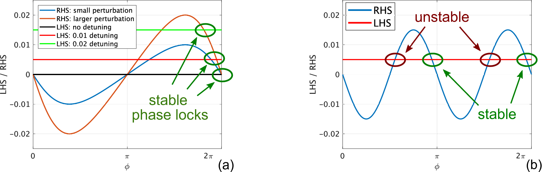
As mentioned in Sec. 1, SHIL can occur when the external input is about twice as fast as the oscillator. When the input is at frequency , it can be shown that the corresponding becomes a -periodic function [14, 32]; a typical example is given in Figure 2 (b), where takes the shape of . In this case, two of the four LHS-RHS intersections represent stable phase-locked states; it can be shown that they are separated by a phase difference of [14]. Gen-Adler is a powerful technique for predicting and understanding injection locking in oscillators and constitutes an important foundation for the analyses that follow.
3.2 Global Lyapunov function
For an oscillator in a coupled oscillator network, its external perturbations come from the other oscillators that are connected to it. Its Gen-Adler equation can be written as
| (5) |
where represents the phases of oscillators; is the frequency of the oscillator whereas is the central frequency of the network. is a -periodic function for the coupling between oscillators and .
To simplify exposition, we now assume that the functions are sinusoidal, although in Appendix A., we show that this does not have to be the case for the analysis to hold true.44 4 More generally, s can be any -periodic odd functions, which are better suited to practical oscillators. We further assume zero spread in the natural frequencies of oscillators, i.e., , and discuss the effect of frequency variability later in Sec. 3.4. With these simplifications, Equation 5 can be written as
| (6) |
Here, we are using the coefficients 55 5 In the Ising Hamiltonian Equation 1, is only defined when ; here we assume that for all . from the Ising model Equation 1 to set the connectivity of the network, i.e., the coupling strength between oscillators and is proportional to . The parameter modulates the overall coupling strength of the network.
There is a global Lyapunov function associated with Equation 6 [33]:
| (7) |
where . Being a global Lyapunov function, it is an objective function the coupled oscillator system always tends to minimise as it evolves over time [34].
If we look at the values of this continuous function at some discrete points, we notice that it shares some similarities with the Ising Hamiltonian. At points where every is equal to either or ,66 6 More generally, we can use and to represent the two states for each oscillator’s phase. if we map to and to , we have
| (8) |
If we choose , the global Lyapunov function in Equation 7 exactly matches the Ising Hamiltonian in Equation 2 at these discrete points. But this does not mean that coupled oscillators are naturally minimising the Ising Hamiltonian, as there is no guarantee at all that the phases are settling to these discrete points. In fact, networks with more than two oscillators almost always synchronise with analog phases, i.e., commonly settle to continuous values spread out in the phase domain as opposed to converging towards and . As an example, Figure 3 (a) shows the phase responses of 20 oscillators connected in a random graph. As phases do not settle to the discrete points discussed above, the Lyapunov function they minimise becomes irrelevant to the Ising Hamiltonian, rendering the system ineffective for solving Ising problems. While one may think that the analog phases can still serve as solutions when rounded to the nearest discrete points, experiments in Sec. 4.2 show that the quality of these solutions is very poor compared with our scheme of Ising machines proposed in this paper.

(a) without SYNC; (b) with .
3.3 Network of coupled oscillators under SHIL and its global Lyapunov function
In our scheme, a common SYNC signal at is injected to every oscillator in the network. Through the mechanism of SHIL, the oscillator phases are binarised. The example shown in Figure 3 (b) confirms that this is indeed the case: under SHIL, the phases of 20 oscillators connected in the same random graph now settle very close to discrete points. To write the model for such a system, we recall from Sec. 3.1 that a perturbation introduces a -periodic coupling term (e.g., ) in the phase dynamics. Therefore, here we can directly write the model as follows and show its derivation in Appendix A..
| (9) |
where represents the strength of coupling from SYNC.
Remarkably, there is a global Lyapunov function for this new type of coupled oscillator system. It can be written as
| (10) |
Now, we show that in Equation 10 is indeed a global Lyapunov function. To do so, we first differentiate with respect to . We observe that the first component of is the sum of number of terms. Among them, for any given index , variable appears a total of times. It appears times as the subtrahend inside : these terms are , where and . For the other times, it appears as the minuend inside : in , where , . So when we differentiate with respect to , we have
| (11) | ||||
| (12) | ||||
| (13) | ||||
| (14) |
Therefore,
| (15) | ||||
| (16) |
Thus, we have proved that Equation 10 is indeed a global Lyapunov function the coupled oscillators under SHIL naturally minimise over time. A similar but more detailed proof for the general case where we do not assume sinusoidal coupling functions is given in Appendix C..
At the discrete points (phase values of 0/), because , Equation 10 reduces to
| (17) |
where is a constant. By choosing , we can then make Equation 17 equivalent to the Ising Hamiltonian in Equation 2 with a constant offset.
Note that the introduction of SYNC does not change the relative levels between the discrete points, but modifies them by the same amount. However, with SYNC, all phases can be forced to eventually take values near either or — the system now tries to reach a binary state that minimises the Ising Hamiltonian, thus functioning as an Ising machine. We emphasise that this is not equivalent to running the system without SHIL and then rounding the analog phase solutions to discrete values as a post-processing step. Instead, the introduction of SHIL modifies the energy landscape of , changes the dynamics of the coupled oscillator system, and as we show in Sec. 4, results in greatly improved minimisation of the Ising Hamiltonian.
It is worth noting, also, that the Lyapunov function in Equation 10 will, in general, have many local minima and there is no guarantee the oscillator-based Ising machine will settle at or near any global optimal state. However, as we show in Appendix B., when judicious amounts of noise are introduced via a noise level parameter , it becomes more likely to settle to lower minima. Indeed, the several parameters in the Ising machine — , and — all play an important role in its operation and should be given suitable values. Furthermore, , , can also be time varying, creating various “annealing schedules”. As we show in Sec. 4, this feature gives us considerable flexibility in operating oscillator-based Ising machines for good performance.
3.4 Coupled oscillator networks with frequency variations
A major obstacle to practical implementation of large-scale Ising machines is variability. While few analyses exist for assessing the effects of variability for previous Ising machine technologies (Sec. 2), the effect of variability on our oscillator-based Ising machine scheme is easy to analyze, predicting that performance degrades gracefully.
One very attractive feature of oscillators is that variability, regardless of the nature and number of elemental physical sources, eventually manifests itself essentially in only one parameter, namely the oscillator’s natural frequency. As a result, the effect of variability in an oscillator network is that there is a spread in the natural frequencies of the oscillators. Taking this into consideration, our model can be revised as
| (18) |
As it turns out, there is also a global Lyapunov function associated with this system.
| (19) |
This can be proven as follows.
| (20) | ||||
| (21) |
Therefore,
| (22) |
Note that Equation 19 differs from Equation 10 only by a weighted sum of — it represents essentially the same energy landscape but tilted linearly with the optimisation variables. While it can still change the locations and values of the solutions, its effects are easy to analyse given a specific combinatorial optimisation problem. Also, as the coupling coefficient gets larger, the effect of variability can be reduced. Small amounts of variability merely perturb the locations of minima a little, i.e., the overall performance of the Ising machine remains essentially unaffected. Very large amounts of variability can, of course, eliminate minima that would exist if there were no variability. However, another great advantage of using oscillators is that even in the presence of large variability, the frequency oscillators can be calibrated (e.g., using a voltage-controlled oscillator (VCO) scheme) prior to each run of the machine. As a result, the spread in frequencies can be essentially eliminated in a practical and easy-to-implement way.
4 Examples
In this section, we demonstrate the feasibility and efficacy of our oscillator-based Ising machine scheme by applying it to several MAX-CUT examples and a graph-colouring problem.
4.1 Small MAX-CUT Problems
Given an undirected graph, the MAX-CUT problem [35, 12] asks us to find a subset of vertices such that the total weights of the cut set between this subset and the remaining vertices are maximised. As an example, Figure 4 shows a size-8 cubic graph, where each vertex is connected to three others — neighbours on both sides and the opposing vertex. As shown in Figure 4, dividing the 8 vertices randomly yields a cut size of 5; grouping even and odd vertices, which one may think is the best strategy, results in a cut size of 8; the maximum cut is actually 10, with one of the solutions shown in the illustration. Changing the edge weights to non-unit values can change the maximum cut and also make the solution look less regular, often making the problem more difficult to solve. While the problem may not seem challenging at size 8, it quickly becomes intractable as the size of the graph grows. In fact, MAX-CUT is one of Karp’s 21 NP-complete problems [10].

The MAX-CUT problem has a direct mapping to the Ising model [10], by choosing to be the opposite of the weight of the edge between vertices and , i.e., . To explain this mapping scheme, we can divide the vertices into two sets — and . Accordingly, all the edges in the graph are separated into three groups — those that connect vertices within , those within , and the cut set containing edges across and . The sums of the weights in these three sets are denoted by , and . Together, they constitute the total edge weights of the graph, which is also the negation of the sum of all the s:
| (23) |
We then map this division of vertices to the values of Ising spins, assigning to a spin if vertex , and if the vertex is in . The Ising Hamiltonian in Equation 2 can then be calculated as
| (24) |
Therefore, when the Ising Hamiltonian is minimised, the cut size is maximised.
To show that an oscillator-based Ising machine can indeed be used to solve MAX-CUT problems, we simulated the Kuramoto model in Equation 9 while making the s represent the unit-weight cubic graph in Figure 4. The magnitude of SYNC is fixed at , while we ramp up the coupling strength from 0 to 5. Results from the deterministic model () and the stochastic model () are shown in Figure 6 and Figure 6 respectively. In the simulations, oscillators started with random phases between 0 and ; after a while, they all settled to one of the two phase-locked states separated by . These two groups of oscillators represent the two subsets of vertices in the solution. The results for the 8 spins shown in Figure 6 and Figure 6 are and respectively; both are global optimal solutions.


A minimal code for reproducing these results is show in Appendix D. Note that these are simulations on stochastic differential equations with random initial conditions. Every run will return different waveforms; there is no guarantee that the global optimum will be reached on every run.

We have also directly simulated coupled oscillators at the SPICE level to confirm the results obtained on phase macromodels. Such simulations are at a lower lever than phase macromodels and are less efficient. But they are closer to physical reality and are useful for circuit design. In the simulations, 8 cross-coupled LC oscillators are tuned to a frequency of 5MHz. They are coupled through resistors, with conductances proportional to the coupling coefficients; in this case, we use . Results from transient simulation using ngspice-28 are shown in Figure 7. The 8 oscillators’ phases settle into the two groups {1,4,6,7} and {2,3,5,8}, representing one of the optimal solutions for the MAX-CUT problem. They synchronise within 20s after oscillation starts, which is about 100 cycles. We have tried this computational experiment with different random initial conditions; like phase-macromodels, the SPICE-level simulations of these coupled oscillators reliably return optimal solutions for this size-8 MAX-CUT problem.

We have also implemented these 8 coupled LC oscillators on a breadboard; a photo of it is shown in Figure 8. The inductance of the LC oscillators is provided by fixed inductors of size 33H. The capacitance is provided by trimmer capacitors with a maximum value of 50pF; we have tuned them to around 30pF such that the natural frequencies of all oscillators are about 5MHz. The nonlinearity for sustaining the LC oscillation is implemented by cross-coupled CMOS inverters on TI SN74HC04N chips. SYNC is supplied through the GND pins of these chips. The results have been observed using two four-channel oscilloscopes; a screenshot of one of them is shown in Figure 8. Through experiments with various sets of edge weights, we have validated that this is indeed a proof-of-concept hardware implementation of oscillator-based Ising machines for size-8 cubic-graph MAX-CUT problems.

Using the same type of oscillators, we have built hardware Ising machines of larger sizes. Figure 9 shows a size-32 example implementing a type of connectivity known as the Chimera graph, much like the quantum Ising machines manufactured by D-Wave Systems. In this graph, oscillators are organised into groups of 8, with denser connections within the groups and sparse ones in between. The hardware is on perfboards, with components soldered on the boards so that the setup is more permanent than those on breadboards. Connections are implemented using rotary potentiometers. Next to each potentiometer we have designed male pin connectors soldered on the board such that the polarity of each connection can be controlled by shorting different pins using female jumper caps. When encoding Ising problems, we have also colour-coded the jumper caps to make debugging easier, as can be seen in the photo as red and green dots next to the four arrays of white round potentiometers. To read the phases of the oscillators, instead of using multichannel oscilloscopes, we have soldered TI SN74HC86N Exclusive-OR (XOR) gate chips on board. The XOR operation of an oscillator’s response and a reference signal converts the oscillating waveform into a high or low voltage level, indicating if the oscillator’s phase is aligned with or opposite to the reference phase. The voltage level can then be picked up by a multichannel logic analyzer. The entire setup is powered by two Digilent Analog Discovery 2 devices, which are portable USB devices that integrate power supplies, logic analyzers and function generators. We have tried random Ising problems by programming each connection with a random polarity using the jumper caps. A typical histogram of the Ising Hamiltonians achieved is shown in Figure 9 (c). Note that because s have random polarities, a random solution would have an average energy level of zero. In comparison, the results measured from the hardware are always below 0, and sometimes achieve the global minimum. While such a hand-soldered system is nontrivial to assemble and operate, and its size of 32 cannot be characterised as large scale, it is a useful proof of concept for implementing oscillator-based Ising machines using standard CMOS technologies, and serves as a very solid basis for our future plans to scale the implementations with custom PCBs and custom ICs.
4.2 MAX-CUT Benchmark Problems
In this section, we demonstrate the efficacy of oscillator-based Ising machines for solving larger-scale MAX-CUT problems. Specifically, we have run simulations on all the problems in a widely used set of MAX-CUT benchmarks known as the G-set [36].77 7 The G-set problems are available for download as set1 at http://www.optsicom.es/maxcut. Problem sizes range from 800 to 3000.88 8 G121 are of size 800; G2242 are of size 2000; G4347, G5154 are of size 1000; G4850 are of size 3000. In the experiments, we operated the Ising machine for all the problems with a single annealing schedule, i.e., we did not tune our Ising machine parameters individually for different problems. Each problem was simulated with 200 random instances. In Table 1, we list the results and runtime alongside those from several heuristic algorithms developed for MAX-CUT — Scatter Search (SS) [37], CirCut [38], and Variable Neighbourhood Search with Path Relinking (VNSPR) [12].99 9 Their results and runtime are available for download at http://www.optsicom.es/maxcut in the “Computational Experiences” section. We also list the performances of simulated annealing from a recent study [35], the only one we were able to find that contains results for all the G-set problems.
| Benchmark | SS | Time | CirCut | Time | VNSPR | Time | SA | Time | OIM | Time | |||
|---|---|---|---|---|---|---|---|---|---|---|---|---|---|
| G1 | 11624 | 139 | 11624 | 352 | 11621 | 22732 | 11621 | 295 | 11624 | 52.6 | 43 | 123 | |
| G2 | 11620 | 167 | 11617 | 283 | 11615 | 22719 | 11612 | 327 | 11620 | 52.7 | 1 | 87 | |
| G3 | 11622 | 180 | 11622 | 330 | 11622 | 23890 | 11618 | 295 | 11622 | 52.4 | 10 | 117 | |
| G4 | 11646 | 194 | 11641 | 524 | 11600 | 24050 | 11644 | 294 | 11646 | 52.7 | 20 | 133 | |
| G5 | 11631 | 205 | 11627 | 1128 | 11598 | 23134 | 11628 | 300 | 11631 | 52.6 | 3 | 121 | |
| G6 | 2165 | 176 | 2178 | 947 | 2102 | 18215 | 2178 | 247 | 2178 | 52.8 | 4 | 46 | |
| G7 | 1982 | 176 | 2003 | 867 | 1906 | 17716 | 2006 | 205 | 2000 | 52.9 | 17 | 21 | |
| G8 | 1986 | 195 | 2003 | 931 | 1908 | 19334 | 2005 | 206 | 2004 | 52.8 | 2 | 26 | |
| G9 | 2040 | 158 | 2048 | 943 | 1998 | 15225 | 2054 | 206 | 2054 | 52.6 | 2 | 2 | |
| G10 | 1993 | 210 | 1994 | 881 | 1910 | 16269 | 1999 | 205 | 2000 | 52.9 | 21 | 58 | |
| G11 | 562 | 172 | 560 | 74 | 564 | 10084 | 564 | 189 | 564 | 6.7 | 6 | 6 | |
| G12 | 552 | 242 | 552 | 58 | 556 | 10852 | 554 | 189 | 556 | 6.3 | 25 | 25 | |
| G13 | 578 | 228 | 574 | 62 | 580 | 10749 | 580 | 195 | 582 | 6.4 | 3 | 3 | |
| G14 | 3060 | 187 | 3058 | 128 | 3055 | 16734 | 3063 | 252 | 3061 | 14.6 | 27 | 91 | |
| G15 | 3049 | 143 | 3049 | 155 | 3043 | 17184 | 3049 | 220 | 3049 | 16.1 | 41 | 145 | |
| G16 | 3045 | 162 | 3045 | 142 | 3043 | 16562 | 3050 | 219 | 3052 | 14.5 | 8 | 53 | |
| G17 | 3043 | 313 | 3037 | 366 | 3030 | 18555 | 3045 | 219 | 3046 | 14.6 | 5 | 52 | |
| G18 | 988 | 174 | 978 | 497 | 916 | 12578 | 990 | 235 | 990 | 14.7 | 3 | 3 | |
| G19 | 903 | 128 | 888 | 507 | 836 | 14546 | 904 | 196 | 906 | 14.5 | 13 | 13 | |
| G20 | 941 | 191 | 941 | 503 | 900 | 13326 | 941 | 195 | 941 | 14.7 | 160 | 160 | |
| G21 | 930 | 233 | 931 | 524 | 902 | 12885 | 927 | 195 | 931 | 14.6 | 10 | 10 | |
| G22 | 13346 | 1336 | 13346 | 493 | 13295 | 197654 | 13158 | 295 | 13356 | 58.7 | 3 | 93 | |
| G23 | 13317 | 1022 | 13317 | 457 | 13290 | 193707 | 13116 | 288 | 13333 | 58.6 | 8 | 54 | |
| G24 | 13303 | 1191 | 13314 | 521 | 13276 | 195749 | 13125 | 289 | 13329 | 59.0 | 6 | 23 | |
| G25 | 13320 | 1299 | 13326 | 1600 | 12298 | 212563 | 13119 | 316 | 13326 | 58.7 | 6 | 45 | |
| G26 | 13294 | 1415 | 13314 | 1569 | 12290 | 228969 | 13098 | 289 | 13313 | 58.9 | 4 | 81 | |
| G27 | 3318 | 1438 | 3306 | 1456 | 3296 | 35652 | 3341 | 214 | 3323 | 59.0 | 18 | 24 | |
| G28 | 3285 | 1314 | 3260 | 1543 | 3220 | 38655 | 3298 | 252 | 3285 | 61.2 | 1 | 5 | |
| G29 | 3389 | 1266 | 3376 | 1512 | 3303 | 33695 | 3394 | 214 | 3396 | 58.9 | 2 | 8 | |
| G30 | 3403 | 1196 | 3385 | 1463 | 3320 | 34458 | 3412 | 215 | 3402 | 59.0 | 12 | 16 | |
| G31 | 3288 | 1336 | 3285 | 1448 | 3202 | 36658 | 3309 | 214 | 3296 | 59.1 | 5 | 15 | |
| G32 | 1398 | 901 | 1390 | 221 | 1396 | 82345 | 1410 | 194 | 1402 | 17.5 | 5 | 5 | |
| G33 | 1362 | 926 | 1360 | 198 | 1376 | 76282 | 1376 | 194 | 1374 | 15.9 | 1 | 1 | |
| G34 | 1364 | 950 | 1368 | 237 | 1372 | 79406 | 1382 | 194 | 1374 | 15.9 | 24 | 24 | |
| G35 | 7668 | 1258 | 7670 | 440 | 7635 | 167221 | 7485 | 263 | 7675 | 37.1 | 5 | 29 | |
| G36 | 7660 | 1392 | 7660 | 400 | 7632 | 167203 | 7473 | 265 | 7663 | 37.6 | 3 | 58 | |
| G37 | 7664 | 1387 | 7666 | 382 | 7643 | 170786 | 7484 | 288 | 7679 | 37.8 | 1 | 15 | |
| G38 | 7681 | 1012 | 7646 | 1189 | 7602 | 178570 | 7479 | 264 | 7679 | 37.7 | 7 | 18 | |
| G39 | 2393 | 1311 | 2395 | 852 | 2303 | 42584 | 2405 | 209 | 2404 | 37.2 | 1 | 1 | |
| G40 | 2374 | 1166 | 2387 | 901 | 2302 | 39549 | 2378 | 208 | 2389 | 38.1 | 7 | 7 | |
| G41 | 2386 | 1017 | 2398 | 942 | 2298 | 40025 | 2405 | 208 | 2401 | 37.8 | 20 | 71 | |
| G42 | 2457 | 1458 | 2469 | 875 | 2390 | 41255 | 2465 | 210 | 2469 | 37.3 | 4 | 4 | |
| G43 | 6656 | 406 | 6656 | 213 | 6659 | 35324 | 6658 | 245 | 6660 | 29.1 | 17 | 129 | |
| G44 | 6648 | 356 | 6643 | 192 | 6642 | 34519 | 6646 | 241 | 6648 | 29.2 | 21 | 129 | |
| G45 | 6642 | 354 | 6652 | 210 | 6646 | 34179 | 6652 | 241 | 6653 | 29.1 | 10 | 53 | |
| G46 | 6634 | 498 | 6645 | 639 | 6630 | 38854 | 6647 | 245 | 6649 | 29.1 | 9 | 13 | |
| G47 | 6649 | 359 | 6656 | 633 | 6640 | 36587 | 6652 | 242 | 6656 | 29.1 | 16 | 91 | |
| G48 | 6000 | 20 | 6000 | 119 | 6000 | 64713 | 6000 | 210 | 6000 | 23.2 | 194 | 194 | |
| G49 | 6000 | 35 | 6000 | 134 | 6000 | 64749 | 6000 | 210 | 6000 | 23.2 | 180 | 180 | |
| G50 | 5880 | 27 | 5880 | 231 | 5880 | 147132 | 5858 | 211 | 5874 | 25.6 | 10 | 94 | |
| G51 | 3846 | 513 | 3837 | 497 | 3808 | 89966 | 3841 | 234 | 3846 | 18.4 | 23 | 68 | |
| G52 | 3849 | 551 | 3833 | 507 | 3816 | 95985 | 3845 | 228 | 3848 | 18.4 | 10 | 49 | |
| G53 | 3846 | 424 | 3842 | 503 | 3802 | 92459 | 3845 | 230 | 3846 | 18.4 | 9 | 102 | |
| G54 | 3846 | 429 | 3842 | 524 | 3820 | 98458 | 3845 | 228 | 3850 | 18.5 | 3 | 40 |
From Table 1, we observe that our oscillator-based Ising machine is indeed effective — it finds best-known cut values for 38 out of the 54 problems, 17 of which are even better than those reported in the above literature. Moreover, in the 200 random instances, the best cut is often reached more than once — the average for all benchmarks is 20 out of 200. If we relax the objective and look at the number of instances where 99.9% of the cut value is reached, represented by , the average is 56, more than a quarter of the total trials. The results can in fact be improved further if we tailor the annealing schedule for each problem. But to show the effectiveness and generality of our scheme, we have chosen to use the same annealing schedule for all the problems.
In the annealing schedule we used, the coupling strength increases linearly, the noise level steps up from 0 to 1, while SYNC’s amplitude ramps up and down multiple times. Such a schedule was chosen empirically and appears to work well for most G-set problems. Figure 10 shows the behaviour of oscillator phases and the instantaneous cut values under this schedule for solving benchmark problem G1 to its best-known cut size. Some MATLABcode to illustrate the annealing schedule is shown in Appendix D. The code uses MATLAB’s SDE solver and is thus much slower than an implementation in C++ we used to generate the results in Table 1. We plan to release all our code as open-source software in the summer of 2019 so that others can verify and build on our work.

The fact that we were using a fixed schedule also indicates that the actual hardware time for the Ising machine to solve all these benchmarks is the same, regardless of problem size and connectivity. Note that in Figure 10, the end time 20 means 20 oscillation cycles, but this end time is predicated on a coupling strength of . The actual value of for each oscillator depends on the PPV function as well as the amplitude of perturbation from other oscillators, as we show in the derivation of Gen-Adler in Appendix A. As an example, for the LC oscillators we use in Sec. 4.1 with 100k resistive coupling, . This indicates that it takes less than 100 cycles for the oscillators to synchronise in phase, which is consistent with measurements. For such a coupled LC oscillator network, a hardware time of 20 in Figure 10 represents approximately 2000 cycles of oscillation; for 5MHz oscillators that takes 0.4ms. If we use GHz nano-oscillators, the computation time can be well within a microsecond. In comparison, the runtime of the several heuristic algorithms listed in Table 1, even with faster CPUs and parallel implementations in the future, is unlikely to ever drop to this range.
As the hardware time is fixed, the runtime we report in Table 1 for our Ising machines is the time for simulating the SDEs of coupled oscillators on CPUs. While we list runtime results for each algorithm in Table 1, note that they come from different sources and are measured on different platforms. Results for SS, CirCut and VNSPR were obtained from Dual Intel Xeon at 3.06GHz with 3.2GB of RAM; SA was run on Intel Xeon E3-1245v2 at 3.4GHz with 32GB of RAM [35]. To make the results generally comparable, we ran our simulations on a modest personal desktop with Intel Xeon E5-1603v3 at 2.8GHz with 16GB of RAM. Even so, it came as a nice surprise to us that even by simulating SDEs we were able to solve the benchmarks efficiently. Another notable feature of our method is that unlike other algorithms, SDE simulation does not know about the Ising Hamiltonian or cut value — it never needs to evaluate the energy function or relative energy changes, which are implicit in the dynamics of differential equations, yet it proves effective and fast.

We also ran more computational experiments on the G-set benchmarks in order to study the mechanism of oscillator-based Ising machines. We created several variants of the Ising machine used above by removing different components in its operation. For each variant, we re-ran 200 random instances for each of the 54 benchmarks, generating 10800 cut values. In Figure 11, we compare the quality of these cut values with results from the unaltered Ising machine by plotting histograms of the distances of the cut values to their respective maxima. In the first variant, we removed noise from the model by setting . The solutions become considerably worse, confirming that noise helps the coupled oscillator system settle to lower energy states.
In the next variant, we removed SYNC by setting . Without SYNC, the system becomes a simple coupled oscillator system with phases that take a continuum of values, as discussed in Sec. 3.2. The settled analog values of the phases that were then thresholded to or to correspond to Ising spins. As shown in Figure 11, the results become significantly worse; indeed, none of the best-known results were reached. This indicates that the SYNC signal and the mechanism of SHIL we introduce to the coupled oscillator networks are indeed essential for them to operate as Ising machines.
Our baseline Ising machine actually uses a smoothed square function for the coupling, as opposed to the used in the original Kuramoto model, as shown in the code in Appendix D. This changes the term in the energy function Equation 10 to a triangle function. Such a change appears to give better results than the original, as shown in Figure 11 (c). The change requires designing oscillators with special PPV shapes and waveforms such that their cross-correlation is a square wave, which is not difficult in practice based on our derivation in Appendix A. As an example, rotary traveling wave oscillators naturally have square PPVs. Ring oscillators can also be designed with various PPVs and waveforms by sizing each stage individually. We cannot say definitively that the square function we have used is optimal for Ising solution performance, but the significant improvement over sinusoidal coupling functions indicates that a fruitful direction for further exploration may be to look beyond the original Kuramoto model for oscillator-based computing.
The last variant we report here added variability to the natural frequencies of the oscillators, as in Equation 18. We assigned Gaussian random variables to s with as the mean, and 0.01 (1%) and 0.05 (5%), respectively, as the standard deviations for two separate runs. From Figure 11 (d), we observe that even with such non-trivial spread in the natural frequencies of oscillators, the performance is affected very little.

Finally, we conducted a preliminary study of the scaling of the time taken by the Ising machine to reach good solutions as problem sizes increase. As the G-set benchmarks have only a few sizes (800, 1000, 2000 and 3000), we used the program (named rudy) that generated them to create more problems of various sizes. All generated problems used random graphs with 10% connectivity and coupling coefficients. We simulated all of them, each for 200 instances, with fixed parameters , , , and show all their Ising Hamiltonians over time in Figure 12. Much to our surprise, the speed in which the values settle appears almost constant, regardless of the problem size. While this does not necessarily mean they all converge to the global optima within the same time, this preliminary study is encouraging as it confirms the massively parallel nature of the system. For larger Ising problems, our Ising machine only needs to scale linearly in hardware size with the number of spins, but does not necessarily require much more time to reach a solution.
4.3 A Graph Colouring Example
As mentioned in Sec. 2, many problems other than MAX-CUT can be mapped to the Ising model [11] and solved by an oscillator-based Ising machine. Here we show an example of a graph colouring problem — assigning four colours to the 51 states (including a federal district) of America such that no two adjacent states have the same colour.
Each state is represented as a vertex in the graph. When two states are adjacent, there is an edge in the graph that connects the corresponding vertices. For every vertex , we assign four spins — , , and siY to represent its colouring scheme; when only one of them is , the vertex is successfully coloured as either red, green, blue or yellow. Then we write an energy function associated with these spins as follows:
| (25) |
where is the number of vertices, represents the edge set, is the number of edges and in this case equal to 220.1010 10 Hawaii and Alaska are considered adjacent such that their colours will be different in the map.
The first term of is a sum of squares never less than zero; it reaches zero only when contains three s and one for every , i.e., each state has a unique colour. The latter term is also a sum that is always greater than or equal to zero, as each spin can only take a value in ; it is zero when never occurs for any edge connecting and , and for any colour , i.e., adjacent states do not share the same colour. Therefore, when reaches its minimum value 0, the spin configuration represents a valid colouring scheme — following the indices of the spins , we can then assign colour to state .

Note that when expanding the sum of squares in Section 4.3, we can use the fact to eliminate the square terms. This means contains only products of two spins — modelled by s, and self terms — modelled by . These Ising coefficients can then be used to determine the couplings in an oscillator-based Ising machine.
We simulated these 204 coupled oscillators and show the results in Figure 13. In the simulation, we kept and constant while ramping up and down 5 times. We found the Ising machine to be effective with this schedule as it could colour the map successfully in more than 50% of the random trials and return many different valid colouring schemes.
Conclusion
In this paper, we have proposed a novel scheme for implementing Ising machines using self-sustaining nonlinear oscillators. We have shown how coupled oscillators naturally minimise an “energy” represented by their global Lyapunov function, and how introducing the mechanism of subharmonic injection locking modifies this function to encode the Ising Hamiltonian for minimisation. The validity and feasibility of the scheme have been examined via multiple levels of simulation and proof-of-concept hardware implementations. Simulations run on larger-scale benchmark problems have also shown promising results in both speed and the quality of solutions. We believe that our scheme constitutes an important and practical means for the implementation of scalable Ising machines.
References
- [1] E. Ising. Beitrag zur theorie des ferromagnetismus. Zeitschrift für Physik A Hadrons and Nuclei, 31(1):253–258, 1925.
- [2] Stephen G. Brush. History of the Lenz-Ising Model. Rev. Mod. Phys., 39:883–893, Oct 1967.
- [3] Francisco Barahona. On the computational complexity of Ising spin glass models. Journal of Physics A: Mathematical and General, 15(10):3241, 1982.
- [4] A. Marandi, Z. Wang, K. Takata, R. L. Byer and Y. Yamamoto. Network of time-multiplexed optical parametric oscillators as a coherent Ising machine. Nature Photonics, 8(12):937–942, 2014.
- [5] P. L. McMahon, A. Marandi, Y. Haribara, R. Hamerly, C. Langrock, S. Tamate and T. Inagaki, H. Takesue, S. Utsunomiya, K. Aihara and others. A fully-programmable 100-spin coherent Ising machine with all-to-all connections. Science, page 5178, 2016.
- [6] T. Inagaki, Y. Haribara, K. Igarashi, T. Sonobe, S. Tamate, T. Honjo, A. Marandi, P. L. McMahon, T. Umeki, K. Enbutsu and others. A Coherent Ising machine for 2000-node Optimization Problems. Science, 354(6312):603–606, 2016.
- [7] M. W. Johnson, M. H. S. Amin, S. Gildert, T. Lanting, F. Hamze, N. Dickson, R. Harris, A. J. Berkley, J. Johansson, P. Bunyk and others. Quantum Annealing with Manufactured Spins. Nature, 473(7346):194, 2011.
- [8] Z. Bian, F. Chudak, R. Israel, B. Lackey, W. G. Macready and A. Roy. Discrete optimization using quantum annealing on sparse Ising models. Frontiers in Physics, 2:56, 2014.
- [9] M. Yamaoka, C. Yoshimura, M. Hayashi, T. Okuyama, H. Aoki and H. Mizuno. A 20k-spin Ising Chip to Solve Combinatorial Optimization Problems with CMOS Annealing. IEEE Journal of Solid-State Circuits, 51(1):303–309, 2016.
- [10] R. M. Karp. Reducibility among combinatorial problems. In Complexity of computer computations, pages 85–103. Springer, 1972.
- [11] A. Lucas. Ising formulations of many NP problems. arXiv preprint arXiv:1302.5843, 2013.
- [12] P. Festa, P. M. Pardalos, M. G. C. Resende, and C. C. Ribeiro. Randomized heuristics for the MAX-CUT problem. Optimization methods and software, 17(6):1033–1058, 2002.
- [13] Tommy R Jensen and Bjarne Toft. Graph Coloring Problems, volume 39. John Wiley & Sons, 2011.
- [14] A. Neogy and J. Roychowdhury. Analysis and Design of Sub-harmonically Injection Locked Oscillators. In Proc. IEEE DATE, Mar 2012. DOI link.
- [15] P. Bhansali and J. Roychowdhury. Gen-Adler: The generalized Adler’s equation for injection locking analysis in oscillators. In Proc. IEEE ASP-DAC, pages 522–227, January 2009. DOI link.
- [16] Yoshiki Kuramoto. Self-entrainment of a population of coupled non-linear oscillators. In International symposium on mathematical problems in theoretical physics, pages 420–422. Springer, 1975.
- [17] Y. Kuramoto. Chemical Oscillations, Waves and Turbulence. Dover, 2003.
- [18] J. A. Acebrón, L. L. Bonilla, C. J. P. Vicente, F. Ritort and R. Spigler. The Kuramoto Model: A Simple Paradigm for Synchronization Phenomena. Reviews of Modern Physics, 77(1):137, 2005.
- [19] T. Wang and J. Roychowdhury. PHLOGON: PHase-based LOGic using Oscillatory Nanosystems. In Proc. UCNC, LNCS sublibrary: Theoretical computer science and general issues. Springer, July 2014. DOI link.
- [20] Maliheh Aramon, Gili Rosenberg, Elisabetta Valiante, Toshiyuki Miyazawa, Hirotaka Tamura, and Helmut G. Katzgraber. Physics-Inspired Optimization for Quadratic Unconstrained Problems Using a Digital Annealer. In arXiv:1806.08815 [physics.comp-ph], August 2018.
- [21] H. Gyoten, M. Hiromoto and T. Sato. Area efficient annealing processor for ising model without random number generator. IEICE Transactions on Information and Systems, E101.D(2):314–323, 2018.
- [22] H. Gyoten, M. Hiromoto and T. Sato. Enhancing the solution quality of hardware ising-model solver via parallel tempering. In Proc. ICCAD, ICCAD ’18, pages 70:1–70:8, New York, NY, USA, 2018. ACM.
- [23] Zhengbing Bian, Fabian Chudak, William G Macready, and Geordie Rose. The Ising model: teaching an old problem new tricks. D-Wave Systems, 2, 2010.
- [24] R. Harris, J. Johansson, A. J. Berkley, M. W. Johnson, T. Lanting, S. Han, P. Bunyk, E. Ladizinsky, T. Oh, I. Perminov and others. Experimental Demonstration of a Robust and Scalable Flux Qubit. Physical Review B, 81(13):134510, 2010.
- [25] T. F. Rønnow, Z. Wang, J. Job, S. Boixo, S. V. Isakov, D. Wecker, J. M. Martinis, D. A. Lidar and M. Troyer. Defining and detecting quantum speedup. Science, 345(6195):420–424, 2014.
- [26] V. S. Denchev, S. Boixo, S. V. Isakov, N. Ding, R. Babbush, V. Smelyanskiy, J. Martinis, H. Neven. What is the computational value of finite-range tunneling? Physical Review X, 6(3):031015, 2016.
- [27] I. Mahboob, H. Okamoto and H. Yamaguchi. An electromechanical Ising Hamiltonian. Science Advances, 2(6):e1600236, 2016.
- [28] K. Y. Camsari, R. Faria, B. M. Sutton and S. Datta. Stochastic p-Bits for Invertible Logic. Physical Review X, 7(3):031014, 2017.
- [29] K. Yamamoto, W. Huang, S. Takamaeda-Yamazaki, M. Ikebe, T. Asai, M. Motomura. A Time-Division Multiplexing Ising Machine on FPGAs. In Proceedings of the 8th International Symposium on Highly Efficient Accelerators and Reconfigurable Technologies, page 3. ACM, 2017.
- [30] A. Winfree. Biological Rhythms and the Behavior of Populations of Coupled Oscillators. Theoretical Biology, 16:15–42, 1967.
- [31] A. Demir, A. Mehrotra, and J. Roychowdhury. Phase Noise in Oscillators: a Unifying Theory and Numerical Methods for Characterization. IEEE Trans. Ckts. Syst. – I: Fund. Th. Appl., 47:655–674, May 2000. DOI link.
- [32] T. Wang and J. Roychowdhury. Design Tools for Oscillator-based Computing Systems. In Proc. IEEE DAC, pages 188:1–188:6, 2015. DOI link.
- [33] S. Shinomoto, Y. Kuramoto. Phase transitions in active rotator systems. Progress of Theoretical Physics, 75(5):1105–1110, 1986.
- [34] A. M. Lyapunov. The General Problem of the Stability of Motion. International Journal of Control, 55(3):531–534, 1992.
- [35] T. Myklebust. Solving maximum cut problems by simulated annealing. arXiv preprint arXiv:1505.03068, 2015.
- [36] C. Helmberg, F. Rendl. A spectral bundle method for semidefinite programming. SIAM Journal on Optimization, 10(3):673–696, 2000.
- [37] R. Martí, A. Duarte, M. Laguna. Advanced scatter search for the max-cut problem. INFORMS Journal on Computing, 21(1):26–38, 2009.
- [38] S. Burer, R. Monteiro, Y. Zhang. Rank-two relaxation heuristics for max-cut and other binary quadratic programs. SIAM Journal on Optimization, 12(2):503–521, 2002.
- [39] R. Adler. A study of locking phenomena in oscillators. Proceedings of the I.R.E. and Waves and Electrons, 34:351–357, June 1946.
- [40] J. Roychowdhury. Exact analytical equations for predicting nonlinear phase errors and jitter in ring oscillators. In Proc. IEEE International Conference on VLSI Design, January 2005.
- [41] A. Demir and J. Roychowdhury. A Reliable and Efficient Procedure for Oscillator PPV Computation, with Phase Noise Macromodelling Applications. IEEE Trans. CAD, pages 188–197, February 2003. DOI link.
- [42] T. Mei and J. Roychowdhury. PPV-HB: Harmonic Balance for Oscillator/PLL Phase Macromodels. In Proc. ICCAD, pages 283–288, Nov. 2006.
- [43] J. Roychowdhury. Applied and Computational Control, Signals and Circuits – Recent Developments, chapter 3 (Multi-time PDEs for Dynamical System Analysis), pages 85–143. Kluwer Academic, 2001.
- [44] R. Adler. A study of locking phenomena in oscillators. Proc. IEEE, 61:1380–1385, 1973. Reprinted from [39].
- [45] L. D. Landau and E. M. Lifshitz. Statistical Physics: V. 5: Course of Theoretical Physics. Pergamon press, 1969.
- [46] R. Yuan, Y. Ma, B. Yuan and P. Ao. Constructive Proof of Global Lyapunov Function as Potential Function. arXiv preprint arXiv:1012.2721, 2010.
Appendix Appendix A. Phase-based Macromodels of Oscillators and Oscillator-based Ising Machines
Studies on the phase dynamics of coupled oscillators commonly start from the Kuramoto model or its variants, which are high-level abstractions. Here in this appendix, we start from low-level oscillator models instead and derive the generalised Kuramoto model for Ising machines from the ground up.
A single nonlinear self-sustaining oscillator is an autonomous dynamical system, usually modelled using Differential Algebraic Equations (DAEs) in the following form.
| (26) |
where represents the unknowns in the system; and are functions, representing the differential and algebraic parts of the DAE respectively.
A self-sustaining oscillator has a nonconstant -periodic solution to Equation 26, satisfying .
When this oscillator is under a time-varying perturbation modelled as , its DAE can be written as follows.
| (27) |
If the perturbation is small, the oscillator’s perturbed response can be approximated well as
| (28) |
where is the phase shift caused by the external input and is governed by the following differential equation [31]:
| (29) |
where the time-varying vector is known as the Perturbation Projection Vector (PPV) [31] of the oscillator. It is -periodic, and is a property intrinsic to the oscillator that captures its phase response to small external inputs. can be derived analytically [40] or calculated numerically [41, 42] from the oscillator’s DAE without knowing any information about the input .
To study injection locking in the oscillator, we assume that the external input is a periodic signal with frequency and a time-varying phase :
| (30) |
where is -periodic function.
Equation Equation 29 can be rewritten as
| (31) |
where — when injection locking occurs, it is the phase shift of the oscillator’s response from a perfect oscillation at . is the -periodic version of the PPV — .
A differential equation such as Equation 30 can be formulated as a Multi-time Partial Differential Equation (MPDE) [43], assuming the oscillation at happens in the fast time whereas the phases evolve in the slow time .
| (32) |
The theory of MPDE states that if we solve the PDE in Appendix Appendix A. for , the solution to the original single-time differential equation Equation 30 can be written as .
We can approximate the MPDE by averaging it along the dimension — replacing the -varying solution with a constant for every . This is usually a valid approximation that does not degrade the accuracy by much, as the phase of oscillation is changing much more slowly than the oscillation itself. In this case, we are approximating the two-dimensional solution with .
| (33) | ||||
| (34) |
To help simplify the equation, we define
| (35) |
is a -periodic function. It is the cross-correlation1111 11 It is also known as the sliding dot product or sliding inner product. of the two functions and .
The one-dimensional solution to Appendix Appendix A. can then be used as an approximation for the solution of . Put in other words, we can rewrite the differential equation Equation 30 for the phase dynamics as
| (36) |
In the case of a common LC oscillator, both its waveform and PPV are sinusoidal. With resistive coupling, its PPV is proportional to [44]. When the perturbation is the same as the oscillator’s waveform, i.e., , the resulting function is proportional to . Then we have rederived the Adler’s equation for LC oscillators.
| (37) |
where the coupling strength is determined mainly by the factor of the LC oscillator.
Another special case is when is a second-order perturbation, i.e., it is oscillating at . We can define another -periodic function , such that . If we further assume that the PPV is also oscillating at twice its natural frequency, i.e., , it can be proven that is also a second-order oscillation.
| (38) | ||||
| (39) | ||||
| (40) | ||||
| (41) |
where is a -periodic function, making is -periodic.
In this special case, the phase dynamics Equation 36 can then be written as
| (42) |
For the th oscillator in an oscillator-based Ising machine, the perturbation to its phase comes from several sources: its connections to the other oscillators, its connection to a reference signal for implementing the self terms in the Ising Hamiltonian, and the second-order SYNC signal. From the above discussion, we can write its phase dynamics as
| (43) |
In equation Appendix Appendix A., is the frequency of this oscillator, is the central frequency for the coupled oscillators. is the -periodic PPV of the th oscillator, with perturbation from the th oscillator, is the -periodic perturbation from the th oscillator. is the -periodic PPV of the th oscillator, with perturbation from a reference signal, is the -periodic reference signal. and represent the waveform of SYNC and the PPV entries corresponding to this second-order perturbation respectively, and are thus both -periodic. We can define , .
Furthermore, we define
| (44) | ||||
| (45) | ||||
| (46) |
Then Appendix Appendix A. can be approximated well with
| (47) |
We can then write the global Lyapunov function as
| (48) |
where , and are defined as follows.
| (49) | ||||
| (50) | ||||
| (51) |
where , and are arbitrary constants.
The generalised Kuramoto model we use in Sec. 3 is just a special case for the phase macromodel we present in this appendix for coupled oscillators. When we need to be functions, we choose to be and use the PPV of harmonic oscillators. In fact, based on the theory we develop in this section, we have all the flexibility to change the shape of periodic functions and . Oscillators can be designed or tweaked to yield the desired energy function.
Appendix Appendix B. Stochastic Model of Oscillator-based Ising Machines
Noise in the phases of oscillators is commonly modelled by adding white noise sources to the oscillator frequencies:
| (53) |
where variable represents Gaussian white noise with a zero mean and a correlator ; scaler represents the magnitude of noise.
Equation 53 can be rewritten as a stochastic differential equation (SDE).
| (54) |
and can then be simulated with standard SDE solvers.
To analyse the steady states of this SDE, we can apply the Boltzmann law from statistical mechanics [45]. For a system with discrete states , , if each state is associated with an energy ,1212 12 It is provable that a global Lyapunov function, if it exists, can be used instead of a physical energy to derive the same Boltzmann law [46]. the probability for the system to be at each state can be written as follows.
| (55) |
where is the Boltzmann constant, is the thermodynamic temperature of the system. While and are concepts specific to statistical mechanics, in this context the product corresponds to the noise level .
Given two spin configurations and , the ratio between their probabilities is known as the Boltzmann factor:
| (56) |
According to the energy function Equation 17 associated with oscillator-based Ising machines, the energy difference that determines this factor is proportional to the coupling strength.
| (57) |
If is the higher energy state, i.e., , as the coupling strength increases, it becomes less and less likely for the system to stay at . The system prefers the lowest energy state in the presence of noise.
Appendix Appendix C. Proof for the global Lyapunov function of oscillator-based Ising machines
Our starting point is the Gen-Adler equation under 2-SHIL (which we have derived elsewhere):
| (58) |
where is the number of coupled oscillators in the system, is the natural frequency of the oscillator, is the phase of the oscillator, is the frequency of the SYNC signal, is the -periodic Adlerized function for the SYNC input to each oscillator, is the symmetric coupling between the and oscillators, and is the -periodic Adlerized function for the coupling inputs to each oscillator.
We assume that every oscillator in the coupled system is sub-harmonically locked to the frequency (more precisely, that remain bounded and small ), and that is skew-symmetric, i.e.,
| (59) |
Define
| (60) |
and
| (61) |
where and are arbitrary constants.
Theorem Appendix C..1
Proof: Using the chain rule of differentiation, we have
| (64) |
Consider . Using Equation 62, we have
| (65) |
We consider the three terms , and in Equation 65 separately, starting with .
| (66) |
where
| (67) |
Hence
| (68) |
Turning to , we have
| (69) |
Finally, for , we have
| (70) |
Using Equation 70, Equation 69 and Equation 68, Equation 65 can be expressed as
| (71) |
Using Equation 71, Equation 64 becomes
| (72) |
Thus, Theorem Appendix C..1 stands proved.
Appendix Appendix D. MATLABSDE Simulation Code for MAX-CUT Problems
-
KuramotoF_sin.m
function fout = KuramotoF_sin(x, Ac, As, n, h, J)for c = 1:nfout(c, 1) = - Ac * h(c) * sin(pi*x(c)) ...- Ac * J(c, :) * sin(pi*(x(c) - x));endfout = (fout - As * sin(2*pi*x))/pi;end
-
run_MAXCUT_8.m
nOsc = 8;h = zeros(nOsc, 1);J = zeros(nOsc, nOsc);J(1, 2) = -1; J(2, 3) = -1; J(3, 4) = -1;J(4, 5) = -1; J(5, 6) = -1; J(6, 7) = -1;J(7, 8) = -1; J(1, 8) = -1; J(1, 5) = -1;J(2, 6) = -1; J(3, 7) = -1; J(4, 8) = -1;J = J + J.’;tstop = 5; tstep = 1e-3;As = 3; Ac = 5; An = 0.1;F = @(t,X) KuramotoF_sin(X, Ac*t/tstop, As, nOsc, h, J);G = @(t,X) An*eye(nOsc);obj = sde(F, G, ’StartState’, rand(nOsc, 1));[S, T] = simulate(obj, tstop/tstep, ’DeltaTime’, tstep);figure; plot(T, S, ’LineWidth’, 2);legend(’\phi_1’, ’\phi_2’, ’\phi_3’, ’\phi_4’, ...’\phi_5’, ’\phi_6’, ’\phi_7’, ’\phi_8’);xlabel(’time (cycles)’); ylabel(’phases (\pi)’);box on; grid on;’
-
KuramotoF.m
function fout = KuramotoF(x, Ac, As, n, h, J)k = 10; % sharpness of square wavefor c = 1:nfout(c, 1) = - Ac * h(c) * tanh(k*sin(pi*x(c))) ...- Ac * J(c, :) * tanh(k*sin(pi*(x(c) - x)));endfout = (fout - As * sin(2*pi*x))/pi;end
-
run_MAXCUT_G1.m
nOsc = 800;h = zeros(nOsc, 1);G22 = importdata(’wherever_set1_is/g1.rud’, ’ ’, 1);p = G22.data(:,1);n = G22.data(:,2);w = G22.data(:,3);W = sparse(p, n, w, nOsc, nOsc);J = - W - W.’;An = 0.8; Ac = 7;tstop = 40; tstep = 2e-3;a1.k = (Ac-1)/tstop;f1 = @(t, args) 1 + t*args.k;a2.T = tstop/20;f2 = @(t, args) 1+2*tanh(10*cos(2*pi*t/args.T));F = @(t,X) KuramotoF(X, f1(t, a1), f2(t, a2), nOsc,h,J);G = @(t,X) An*eye(nOsc);obj = sde(F, G, ’StartState’, rand(nOsc, 1));[S, T] = simulate(obj, tstop/tstep, ’DeltaTime’, tstep);figure; plot(T, S); box on; grid on;cuts = T;for k = 1:length(T)ix = find(mod(round(S(k,:)), 2));cuts(k) = -sum(sum(J(ix, setdiff(1:nOsc, ix))));endfigure; plot(T, cuts);’