Dirichlet Boundary Value Correction using Lagrange Multipliers

Erik Burman Affiliation: Department of Mathematics, University College London, Gower Street, London WC1E 6BT, UK Peter Hansbo Affiliation: Department of Mechanical Engineering, Jönköping University, SE-551 11 Jönköping, Sweden Affiliation: Department of Mathematics and Mathematical Statistics, Umeå University, SE-901 87 Umeå, Sweden Mats G. Larson Affiliation: e.burman@ucl.ac.uk Affiliation: peter.hansbo@ju.se Affiliation: mats.larson@umu.se

August 11, 2026

Abstract

We propose a boundary value correction approach for cases when curved boundaries are approximated by straight lines (planes) and Lagrange multipliers are used to enforce Dirichlet boundary conditions. The approach allows for optimal order convergence for polynomial order up to 3. We show the relation to the Taylor series expansion approach used by Bramble, Dupont and Tomée [4] in the context of Nitsche’s method and, in the case of inf–sup stable multiplier methods, prove a priori error estimates with explicit dependence on the meshsize and distance between the exact and approximate boundary.

1 Introduction

In this contribution we develop a modified Lagrange multiplier method based on the idea of boundary value correction originally proposed for standard finite element methods on an approximate domain in [4] and further developed in [8]. More recently boundary value correction have been developed for cut and immersed finite element methods [6, 7, 2, 12, 13]. Using the closest point mapping to the exact boundary, or an approximation thereof, the boundary condition on the exact boundary may be weakly enforced using multipliers on the boundary of the approximate domain. Of particular practical importance in this context is the fact that we may use a piecewise linear approximation of the boundary, which is very convenient from a computational point of view since the geometric computations are simple in this case and a piecewise linear distance function may be used to construct the discrete domain.

We prove optimal order a priori error estimates, in the energy and $L^{2}$ norms, in terms of the error in the boundary approximation and the meshsize. The proof utilizes the a priori error estimates derived in [6] for the cut boundary value corrected Nitsche method together with a bound, which shows that the solution to the boundary value corrected Lagrange method is close to the corresponding Nitsche solution for which optimal bounds are available. We obtain optimal order convergence for polynomial approximation up to order 3 of the solution.

Note that without boundary correction one typically requires $O(h^{p+1})$ accuracy in the $L^{\infty}$ norm for the approximation of the domain, which leads to significantly more involved computations on the cut elements for higher order elements, see [10]. We present numerical results illustrating our theoretical findings.

The outline of the paper is as follows: In Section 2 we formulate the model problem and our method, in Section 3 we present our theoretical analysis, in Section 4 we discuss the choice of finite element spaces in cut finite element methods, in Section 5 we present the numerical results, and finally in Section 6 we include some concluding remarks.

2 Model problem and method

2.1 The domain

Let $\Omega$ be a domain in $\mathbb{R}^{d}$ with smooth boundary $\partial\Omega$ and exterior unit normal $\bm{n}$ . We let $\varrho$ be the signed distance function, negative on the inside and positive on the outside, to $\partial\Omega$ and we let $U_{\delta}(\partial\Omega)$ be the tubular neighborhood $\{\bm{x}\in\mathbb{R}^{d}:|\varrho(\bm{x})|<\delta\}$ of $\partial\Omega$ . Then there is a constant $\delta_{0}>0$ such that the closest point mapping $\bm{p}(\bm{x}):U_{\delta_{0}}(\partial\Omega)\rightarrow\partial\Omega$ is well defined and we have the identity $\bm{p}(\bm{x})=\bm{x}-\varrho(\bm{x})\bm{n}(\bm{p}(\bm{x}))$ . We assume that $\delta_{0}$ is chosen small enough that $\bm{p}(\bm{x})$ is well defined. See [9], Section 14.6 for further details on distance functions.

2.2 The model problem

We consider the problem: find $u:\Omega\rightarrow\mathbb{R}$ such that

	$\displaystyle-\Delta u$	$\displaystyle=f\qquad$		in $\Omega$		(2.1)
	$\displaystyle u$	$\displaystyle=g\qquad$		on $\partial\Omega$		(2.2)

where $f\in H^{-1}(\Omega)$ and $g\in H^{1/2}(\partial\Omega)$ are given data. It follows from the Lax-Milgram Lemma that there exists a unique solution to this problem and we also have the elliptic regularity estimate

\|u\|_{H^{s+2}(\Omega)}\lesssim\|f\|_{H^{s}(\Omega)},\qquad s\geq-1.

(2.3)

Here and below we use the notation $\lesssim$ to denote less or equal up to a constant.

Using a Lagrange multiplier to enforce the boundary condition we can write the weak form of (2.4)–(2.5) as: find $(u,\lambda)\in H^{1}(\Omega)\times H^{-1/2}(\partial\Omega)$ such that

	$\displaystyle\int_{\Omega}\nabla u\cdot\nabla v\,\text{d}\Omega+\int_{\partial\Omega}\lambda\,v\,\text{d}s$	$\displaystyle=\int_{\Omega}fv\,\text{d}\Omega\qquad\forall v\in H^{1}(\Omega)$		(2.4)
	$\displaystyle\int_{\partial\Omega}u\,\mu\,\text{d}s$	$\displaystyle=\int_{\partial\Omega}g\,\mu\,\text{d}s\qquad\forall\mu\in H^{-1/2}(\partial\Omega)$		(2.5)

2.3 The mesh and the discrete domain

Let $\mathcal{K}_{h},h\in(0,h_{0}]$ , be a family of quasiuniform partitions, with mesh parameter $h$ , of $\Omega$ into shape regular triangles or tetrahedra $K$ . The partitions induce discrete polygonal approximations $\Omega_{h}=\cup_{K\in\mathcal{K}_{h}}K$ , $h\in(0,h_{0}]$ , of $\Omega$ . We assume neither $\Omega_{h}\subset\Omega$ nor $\Omega\subset\Omega_{h}$ , instead the accuracy with which $\Omega_{h}$ approximates $\Omega$ will be crucial. To each $\Omega_{h}$ is associated a discrete unit normal $\bm{n}_{h}$ and a discrete signed distance $\varrho_{h}:\partial\Omega_{h}\rightarrow\mathbb{R}$ , such that if $\bm{p}_{h}(\bm{x},\varsigma):=\bm{x}+\varsigma\bm{n}_{h}(\bm{x})$ then $\bm{p}_{h}(\bm{x},\varrho_{h}(\bm{x}))\in\partial\Omega$ for all $\bm{x}\in\partial\Omega_{h}$ . We will also assume that $\bm{p}_{h}(\bm{x},\varsigma)\in U_{\delta_{0}}(\Omega):=U_{\delta_{0}}(\partial\Omega)\cup\Omega$ for all $\bm{x}\in\partial\Omega_{h}$ and all $\varsigma$ between $0$ and $\varrho_{h}(\bm{x})$ . For conciseness we will drop the second argument of $\bm{p}_{h}$ below whenever it takes the value $\varrho_{h}(\bm{x})$ , and thus we have the map $\partial\Omega_{h}\ni\bm{x}\mapsto\bm{p}_{h}(\bm{x})\in\partial\Omega$ . We assume that the following assumptions are satisfied

\delta_{h}:=\|\varrho_{h}\|_{L^{\infty}(\partial\Omega_{h})}=o(h),\qquad h\in(0,h_{0}]

(2.6)

and

\|\bm{n}_{h}-\bm{n}\circ\bm{p}_{h}\|_{L^{\infty}(\partial\Omega_{h})}=o(1),\qquad h\in(0,h_{0}]

(2.7)

where $o(\cdot)$ denotes the little ordo. We also assume that $h_{0}$ is small enough to guarantee that

\partial\Omega_{h}\subset U_{\delta_{0}}(\partial\Omega),\qquad h\in(0,h_{0}]

(2.8)

and that there exists $M>0$ such for any $\bm{y}\in U_{\delta_{0}}(\partial\Omega)$ the equation, find $\bm{x}\in\partial\Omega_{h}$ and $|\varsigma|\leq\delta_{h}$ such that

{\bm{p}}_{h}(\bm{x},\varsigma)=\bm{y}

(2.9)

has a solution set $\mathcal{P}_{h}$ with

\mbox{card}(\mathcal{P}_{h})\leq M

(2.10)

uniformly in $h$ . The rationale of this assumption is to ensure that the image of $\bm{p}_{h}$ can not degenerate for vanishing $h$ ; for more information cf. [6].

We note that it follows from (2.6) that

\|\varrho\|_{L^{\infty}(\partial\Omega_{h})}\lesssim\|\varrho_{h}\|_{L^{\infty}(\partial\Omega_{h})}=o(h)

(2.11)

since $|\varrho_{h}(\bm{x})|\geq|\varrho(\bm{x})|$ , $\bm{x}\in U_{\delta_{0}}(\partial\Omega)$ . We also assume the additional regularity

f+\Delta u\in H^{l{\color[rgb]{0,0,0}+\frac{1}{2}+\epsilon}}(U_{\delta_{0}}(\Omega))

(2.12)

2.4 The finite element method

2.4.1 Boundary value correction

The basic idea of the boundary value correction of [4] is to use a Taylor series at $\bm{x}\in{\partial\Omega_{h}}$ in the direction $\bm{n}_{h}$ , and let this series represent $u_{h}|_{\partial\Omega}$ . In the present work we will restrict ourselves to

u_{h}\circ\bm{p}_{h}(\bm{x})\approx u_{h}(\bm{x})+\varrho_{h}(\bm{x})\bm{n}_{h}(\bm{x})\cdot\nabla u_{h}(\bm{x})

(2.13)

which is the case of most practical interest.

Choosing appropriate discrete spaces $V_{h}$ and $\Lambda_{h}$ for the approximation of $u$ and $\lambda$ , respectively (particular choices are considered in Section 5), we thus seek $(u_{h},\lambda_{h})\in V_{h}\times\Lambda_{h}$ such that

	$\displaystyle\int_{\Omega_{h}}\nabla u_{h}\cdot\nabla v\,\text{d}\Omega_{h}+\int_{\partial\Omega_{h}}\lambda_{h}\,v\,\text{d}s$	$\displaystyle=\int_{\Omega_{h}}fv\,\text{d}\Omega_{h}\qquad\forall v\in V_{h}$		(2.14)
	$\displaystyle\int_{\partial\Omega_{h}}(u_{h}+\varrho_{h}\bm{n}_{h}\cdot\nabla u_{h})\,\mu\,\text{d}s$	$\displaystyle=\int_{\partial\Omega_{h}}\tilde{g}\,\mu\,\text{d}s\qquad\forall\mu\in\Lambda_{h}$		(2.15)

where we introduced the notation $\tilde{g}:=g\circ\bm{p}_{h}$ for the pullback of $g$ from $\partial\Omega$ to $\partial\Omega_{h}$ .

Using Green’s formula we note that the first equation implies that $\lambda_{h}=-\bm{n}_{h}\cdot\nabla u_{h}$ , and therefore we now propose the following modified method: Find $(u_{h},\lambda_{h})\in V_{h}\times\Lambda_{h}$ such that

	$\displaystyle\int_{\Omega_{h}}\nabla u_{h}\cdot\nabla v\,\text{d}\Omega_{h}+\int_{\partial\Omega_{h}}\lambda_{h}\,v\,\text{d}s$	$\displaystyle=\int_{\Omega_{h}}fv\,\text{d}\Omega_{h}\qquad\forall v\in V_{h}$		(2.16)
	$\displaystyle\int_{\partial\Omega_{h}}u_{h}\,\mu\,\text{d}s-\int_{\partial\Omega_{h}}\varrho_{h}\lambda_{h}\,\mu\,\text{d}s$	$\displaystyle=\int_{\partial\Omega}\tilde{g}\,\mu\,\text{d}s\qquad\forall\mu\in\Lambda_{h}$		(2.17)

A(u_{h},\lambda_{h};v,\mu)=(f,v)_{\Omega_{h}}+(\tilde{g},\mu)_{\partial\Omega_{h}}\quad\forall(u_{h},\lambda_{h})\in V_{h}\times\Lambda_{h}

(2.18)

where $(\cdot,\cdot)_{M}$ denotes the $L_{2}$ scalar product over $M$ , with $\|\cdot\|_{M}$ the corresponding $L_{2}$ norm, and

A(u,\lambda;v,\mu):=(\nabla u,\nabla v)_{\Omega_{h}}+(\lambda,v)_{\partial\Omega_{h}}+(u,\mu)_{\partial\Omega_{h}}-(\varrho_{h}\lambda,\mu)_{\partial\Omega_{h}}.

2.5 Relation to Nitsche’s method with boundary value correction

Problem (2.18) can equivalently be formulated as finding the stationary points of the Lagrangian

\mathcal{L}(u,\lambda):=\frac{1}{2}\|\nabla u\|^{2}_{\Omega_{h}}+(\lambda,u)_{\partial\Omega_{h}}-\|\varrho^{1/2}_{h}\lambda\|^{2}_{\partial\Omega_{h}}-(f,u)_{\Omega_{h}}-(\tilde{g},\lambda)_{\partial\Omega_{h}}

(2.19)

We now follow [5] and add a consistent penalty term and seek stationary points of the augmented Lagrangian

\mathcal{L}_{\text{aug}}(u,\lambda):=\mathcal{L}(u,\lambda)+\frac{1}{2}\|\gamma^{1/2}(u-\varrho_{h}\lambda-\tilde{g})\|^{2}_{\partial\Omega_{h}}

(2.20)

where $\gamma>0$ remains to be chosen. The corresponding optimality system is

	$\displaystyle(f,v)_{\Omega_{h}}+(\tilde{g},\mu)_{\partial\Omega_{h}}={}$	$\displaystyle A(u_{h},\lambda_{h};v,\mu)+(\gamma(u_{h}-\varrho_{h}\lambda_{h}-\tilde{g}),v)_{\partial\Omega_{h}}$
		$\displaystyle-(\gamma\varrho_{h}(u_{h}-\varrho_{h}\lambda_{h}-\tilde{g}),\mu)_{\partial\Omega_{h}}$		(2.21)

Now, formally replacing $\lambda_{h}$ by $-\bm{n}_{h}\cdot\nabla u_{h}$ and $\mu$ by $-\bm{n}_{h}\cdot\nabla v$ we obtain

$\displaystyle(f,v)_{\Omega_{h}}-(\tilde{g},\bm{n}_{h}\cdot\nabla v)_{\partial\Omega_{h}}={}$	$\displaystyle(\nabla u_{h},\nabla v)_{\Omega_{h}}-(\bm{n}_{h}\cdot\nabla u_{h},v)_{\partial\Omega_{h}}$
	$\displaystyle-(u_{h},\bm{n}_{h}\cdot\nabla v)_{\partial\Omega_{h}}-(\varrho_{h}\bm{n}_{h}\cdot\nabla u_{h},\bm{n}_{h}\cdot\nabla v)_{\partial\Omega_{h}}$
	$\displaystyle+(\gamma(u_{h}+\varrho_{h}\bm{n}_{h}\cdot\nabla u_{h}-\tilde{g}),v+\varrho_{h}\bm{n}_{h}\cdot\nabla v)_{\partial\Omega_{h}}$	(2.22)

Setting now $\gamma=\gamma_{0}/h$ , with $\gamma_{0}$ sufficiently large to ensure coercivity, we obtain the symmetrized version of the boundary value corrected Nitsche method proposed in [4] with optimal convergence up to order $p=3$ assuming $\varrho_{h}\geq-Ch$ , for some sufficiently small constant. This means that $\partial\Omega_{h}$ either has to be a good approximation of $\partial\Omega$ , or where it approximates poorly, $\Omega_{h}$ must approximation $\Omega$ from the inside. For future reference we define this method as: Find $u_{h}\in V_{h}$ such that

A_{Nit}(u_{h},v_{h})=(f,v_{h})_{\partial\Omega_{h}}+(\tilde{g},\bm{n}_{h}\cdot\nabla v_{h})_{\partial\Omega_{h}}+(\gamma\tilde{g},v_{h}+\varrho_{h}\bm{n}_{h}\cdot\nabla v_{h})_{\partial\Omega_{h}}

(2.23)

for all $v_{h}\in V_{h}$ . Here the bilinear form is defined by

	$\displaystyle A_{Nit}(w_{h},v_{h})$	$\displaystyle:=(\nabla w_{h},\nabla v_{h})_{\Omega_{h}}-(\bm{n}_{h}\cdot\nabla w_{h},v_{h}+\varrho_{h}\bm{n}_{h}\cdot\nabla v_{h})_{\partial\Omega_{h}}-(w_{h}+\varrho_{h}\bm{n}_{h}\cdot\nabla w_{h},\bm{n}_{h}\cdot\nabla v)_{\partial\Omega_{h}}$
		$\displaystyle\qquad+(\varrho_{h}\bm{n}_{h}\cdot\nabla w_{h},\bm{n}_{h}\cdot\nabla v)_{\partial\Omega_{h}}+(\gamma(w_{h}+\varrho_{h}\bm{n}_{h}\cdot\nabla w_{h},v+\varrho_{h}\bm{n}_{h}\cdot\nabla v_{h})_{\partial\Omega_{h}}.$		(2.24)

3 Elements of analysis

In this section we will prove some basic results on the stability and the accuracy of the method (2.18). We will restrict ourselves to a discussion of the case $-Ch\leq\varrho_{h}$ , for some $C$ small enough. We assume that $\Lambda_{h}$ is the space of piecewise polynomial functions of order $k-1$ and $V_{h}$ is the space of continuous piecewise polynomial functions of order $k$ , that we will denote $V_{h}^{k}$ , enriched with higher order bubbles on the faces in $\partial\Omega_{h}$ so that inf-sup stability holds. The precise condition is given in equation (3.6) below. For details on stable choices of the multiplier space we refer to [1, 3, 11]. We introduce the triple norm defined on $H^{1}(\Omega_{h})\times L^{2}(\partial\Omega_{h})$ :

|\mspace{-1mu}|\mspace{-1mu}|(v,\mu)|\mspace{-1mu}|\mspace{-1mu}|:=\|\nabla v\|_{\Omega_{h}}+\|h^{-\frac{1}{2}}v\|_{\partial\Omega_{h}}+\|h^{\frac{1}{2}}\mu\|_{\partial\Omega_{h}}.

(3.1)

We let $\pi_{h}:L^{2}(\partial\Omega_{h})\to\Lambda_{h}$ denote the $L^{2}$ -orthogonal projection and we assume that the bound

\|v-\pi_{h}v\|_{\partial\Omega_{h}}\lesssim h\|\nabla_{\partial}v\|_{\partial\Omega_{h}}

(3.2)

for all $v\in H^{1}(\partial\Omega_{h})$ and where $\nabla_{\partial}$ denotes the gradient on the boundary. The formulation (2.18) satisfies the following stability result

Proposition 3.1.

Assume that $\varrho_{h}\geq-C_{\partial\Omega}h$ and that $V_{h}\times\Lambda_{h}$ satisfies the inf-sup condition. Then for $C_{\partial\Omega}$ sufficiently small, for all $(y_{h},\eta_{h})\in V_{h}\times\Lambda_{h}$ , there exists $(v_{h},\mu_{h})\in V_{h}\times\Lambda_{h}$ such that

|\mspace{-1mu}|\mspace{-1mu}|(y_{h},\eta_{h})|\mspace{-1mu}|\mspace{-1mu}|\lesssim A(y_{h},\eta_{h};v_{h},\mu_{h})

(3.3)

and

|\mspace{-1mu}|\mspace{-1mu}|(v_{h},\mu_{h})|\mspace{-1mu}|\mspace{-1mu}|\lesssim|\mspace{-1mu}|\mspace{-1mu}|(y_{h},\eta_{h})|\mspace{-1mu}|\mspace{-1mu}|.

(3.4)

Proof.First observe that

A(y_{h},\eta_{h};y_{h},-\eta_{h})=\|\nabla y_{h}\|^{2}_{\Omega_{h}}+(\varrho_{h}\eta_{h},\eta_{h})_{\partial\Omega_{h}}.

(3.5)

Then recall that since the space satisfies the inf-sup condition there exists $v_{\eta}\in V_{h}$ such that

\|h^{\frac{1}{2}}\eta_{h}\|_{\partial\Omega_{h}}\lesssim(\eta_{h},v_{\eta})_{\partial\Omega_{h}}\quad\mbox{and}\quad\|\nabla v_{\eta}\|_{\Omega_{h}}+\|h^{-\frac{1}{2}}v_{\eta}\|_{\partial\Omega_{h}}\lesssim\|h^{\frac{1}{2}}\eta_{h}\|_{\partial\Omega_{h}}.

(3.6)

It follows that for some $c_{\eta},\,C_{\partial\Omega_{h}}$ sufficiently small

	$\displaystyle\\|\nabla y_{h}\\|^{2}_{\Omega_{h}}+\\|h^{\frac{1}{2}}\eta_{h}\\|^{2}_{\partial\Omega}$	$\displaystyle\lesssim\\|\nabla y_{h}\\|^{2}_{\Omega_{h}}+(\varrho_{h}\eta_{h},\eta_{h})_{\partial\Omega_{h}}+\\|h^{\frac{1}{2}}\eta_{h}\\|^{2}_{\partial\Omega}$		(3.7)
		$\displaystyle\lesssim A(y_{h},\eta_{h};y_{h}+c_{\eta}v_{\eta},-\eta_{h}).$		(3.8)

Here we used equation (3.6),

(\varrho_{h}\eta_{h},\eta_{h})_{\partial\Omega_{h}}+\|h^{\frac{1}{2}}\eta_{h}\|^{2}_{\partial\Omega}\geq(1-C_{\partial\Omega_{h}})\|h^{\frac{1}{2}}\eta_{h}\|^{2}_{\partial\Omega}

(3.9)

and

(\nabla y_{h},y_{h}+c_{\eta}v_{\eta})_{\Omega_{h}}\geq-\frac{1}{2}\|\nabla y_{h}\|^{2}_{\Omega_{h}}-2c_{\eta}^{2}\|v_{\eta}\|^{2}_{\partial\Omega}.

(3.10)

Finally let $\mu_{y}=\pi_{h}y_{h}$ and observe that

		$\displaystyle(y_{h},h^{-1}\mu_{y})_{\partial\Omega}-(\rho_{h}\eta_{h},h^{-1}\mu_{y})_{\partial\Omega}$
		$\displaystyle\qquad\geq\\|h^{-\frac{1}{2}}y_{h}\\|_{\partial\Omega_{h}}^{2}-\\|h^{-\frac{1}{2}}(y_{h}-\mu_{y})\\|_{\partial\Omega_{h}}^{2}-\frac{1}{2}C_{\partial\Omega_{h}}^{2}\\|h^{\frac{1}{2}}\eta_{h}\\|_{\partial\Omega_{h}}^{2}-\frac{1}{2}\\|h^{-\frac{1}{2}}\mu_{y}\\|_{\partial\Omega_{h}}^{2}$		(3.11)
		$\displaystyle\qquad\geq\frac{1}{2}\\|h^{-\frac{1}{2}}y_{h}\\|_{\partial\Omega_{h}}^{2}-C^{2}_{t}\\|\nabla y_{h}\\|^{2}_{\Omega_{h}}-\frac{1}{2}C_{\partial\Omega}^{2}\\|h^{\frac{1}{2}}\eta_{h}\\|_{\partial\Omega_{h}}^{2}.$		(3.12)

Where we used the approximation property of $\pi_{h}$ and a trace inequality

h_{K}^{\frac{1}{2}}\|v_{h}\|_{\partial K}+h_{K}\|\nabla v_{h}\|_{K}\lesssim\|v_{h}\|_{K}.

(3.13)

for all elements $K\in\mathcal{K}_{h}$ and polynomials $v_{h}\in\mathbb{P}(K)$ , to show that

\|h^{-\frac{1}{2}}(y_{h}-\mu_{y})\|_{\partial\Omega_{h}}\leq C_{t}\|\nabla y_{h}\|_{\Omega_{h}}.

(3.14)

The first claim follows by taking $v_{h}=y_{h}+c_{\eta}v_{\eta}$ and $\mu_{h}=-\eta_{h}+c_{y}h^{-1}\mu_{y}$ with $c_{\eta}$ and $c_{y}$ both $O(1)$ , sufficiently small and assuming that $C_{\partial\Omega_{h}}$ is small enough.

To conclude the proof we need to show that

|\mspace{-1mu}|\mspace{-1mu}|(v_{h},\mu_{h})|\mspace{-1mu}|\mspace{-1mu}|\lesssim|\mspace{-1mu}|\mspace{-1mu}|(y_{h},\eta_{h})|\mspace{-1mu}|\mspace{-1mu}|.

(3.15)

By the triangle inequality we have

|\mspace{-1mu}|\mspace{-1mu}|(v_{h},\mu_{h})|\mspace{-1mu}|\mspace{-1mu}|\leq|\mspace{-1mu}|\mspace{-1mu}|(y_{h},\eta_{h})|\mspace{-1mu}|\mspace{-1mu}|+|\mspace{-1mu}|\mspace{-1mu}|(c_{\eta}v_{\eta},c_{y}h^{-1}\mu_{y})|\mspace{-1mu}|\mspace{-1mu}|.

(3.16)

By definition

|\mspace{-1mu}|\mspace{-1mu}|(c_{\eta}v_{\eta},c_{y}h^{-1}\mu_{y})|\mspace{-1mu}|\mspace{-1mu}|=c_{\eta}\|\nabla v_{\eta}\|_{\Omega_{h}}+c_{\eta}\|h^{-\frac{1}{2}}v_{\eta}\|_{\partial\Omega_{h}}+c_{y}\|h^{-\frac{1}{2}}\mu_{y}\|_{\partial\Omega_{h}}

(3.17)

and the proof follows from (3.6) together with the stability of $\pi_{h}$ in $L^{2}$ . ∎We will now use this stability result to prove an error estimate. For simplicity we here assume that $\varrho_{h}>0$ , i.e. $\Omega_{h}\subset\Omega$ .

Theorem 3.1.

Let $u\in H^{k+1}(\Omega)$ denote the solution to (2.4)–(2.5). Let $u_{h},\lambda_{h}\in V_{h}\times\Lambda_{h}$ denote the solution of (2.18). Assume that the polynomial order of $V_{h}$ is $k\in\{1,2,3\}$ , with enrichment on the boundary and $\Lambda_{h}\equiv X_{h}^{k-1}$ . Assume that $V_{h}\times\Lambda_{h}$ satisfies (3.6). Then there holds, with $\tilde{\lambda}=\bm{n}_{h}\cdot\nabla u|_{\partial\Omega_{h}}$ ,

	$\displaystyle\|\mspace{-1mu}\|\mspace{-1mu}\|(u-u_{h},\tilde{\lambda}-\lambda_{h})\|\mspace{-1mu}\|\mspace{-1mu}\|$	$\displaystyle\lesssim h^{k}\\|u\\|_{H^{k+1}(\Omega)}+h^{-1/2}\delta_{h}^{2}\sup_{0\leq t\leq\delta_{0}}\\|D^{k+1}u\\|_{L^{2}(\partial\Omega_{t})}$		(3.18)
		$\displaystyle\qquad+{\color[rgb]{0,0,0}h^{1/2}}\delta_{h}^{l+1}\sup_{-\delta_{0}\leq t<0}\\|D_{n}^{l}(f+\Delta u)\\|_{L^{2}(\partial\Omega_{t})}.$

Proof.Let $\tilde{u}_{h}\in V_{h}$ denote the solution to (2.23). We recall from [4, 6] that the following error bound holds

$\displaystyle\|\mspace{-1mu}\|\mspace{-1mu}\|(u-\tilde{u}_{h},0)\|\mspace{-1mu}\|\mspace{-1mu}\|$	$\displaystyle+\\|h^{\frac{1}{2}}\bm{n}_{h}\cdot\nabla(u-\tilde{u}_{h})\\|_{\partial\Omega_{h}}+\\|h^{-\frac{1}{2}}(\tilde{u}_{h}+\varrho\bm{n}_{h}\cdot\nabla\tilde{u}_{h}-\tilde{g})\\|_{\partial\Omega_{h}}$
	$\displaystyle\lesssim h^{k}\\|u\\|_{H^{k+1}(\Omega)}+h^{-1/2}\varrho_{h}^{2}\sup_{0\leq t\leq\delta_{0}}\\|D^{k+1}u\\|_{L^{2}(\partial\Omega_{t})}$	(3.19)
	$\displaystyle\qquad+{\color[rgb]{0,0,0}h^{1/2}}\varrho_{h}^{l+1}\sup_{-\delta_{0}\leq t<0}\\|D_{n}^{l}(f+\Delta u)\\|_{L^{2}(\partial\Omega_{t})}.$

Let $i_{h}u$ denote the nodal interpolant of $u$ . We then form the discrete errors $e_{h}=u_{h}-\tilde{u}_{h}$ and $\varsigma_{h}=\lambda_{h}-\zeta_{h}$ for some $\zeta_{h}\in\Lambda_{h}$ . Using the triangle inequality and we have

|\mspace{-1mu}|\mspace{-1mu}|(u-u_{h},\tilde{\lambda}-\lambda_{h})|\mspace{-1mu}|\mspace{-1mu}|\leq|\mspace{-1mu}|\mspace{-1mu}|(u-\tilde{u}_{h},\tilde{\lambda}-\zeta_{h})|\mspace{-1mu}|\mspace{-1mu}|+|\mspace{-1mu}|\mspace{-1mu}|(e_{h},\varsigma_{h})|\mspace{-1mu}|\mspace{-1mu}|.

(3.20)

Since the first term on the left hand side is bounded by standard interpolation and (3.19). We only need to consider the second term. By the stability estimate of Proposition 3.1 we have

|\mspace{-1mu}|\mspace{-1mu}|(e_{h},\varsigma_{h})|\mspace{-1mu}|\mspace{-1mu}|\lesssim A(e_{h},\varsigma_{h};v_{h},\mu_{h}).

(3.21)

Using the method (2.18) and the definition of $\tilde{u}_{h}$ we find that

$\displaystyle A(e_{h},\varsigma_{h};v_{h},\mu_{h})$	$\displaystyle=(f,v_{h})_{\Omega_{h}}+(\tilde{g},\mu_{h})_{\partial\Omega_{h}}$	(3.22)
	$\displaystyle\qquad-(\nabla\tilde{u}_{h},\nabla v_{h})_{\Omega_{h}}+(\zeta_{h},v_{h})_{\partial\Omega_{h}}$
	$\displaystyle\qquad-(\tilde{u}_{h},\mu_{h})_{\partial\Omega_{h}}-(\varrho_{h}\zeta_{h},\mu_{h})_{\partial\Omega_{h}}.$

The definition of Nitsche’s method (2.23) implies the equality

$\displaystyle(f,v_{h})_{\Omega_{h}}-(\nabla\tilde{u}_{h},\nabla v_{h})_{\Omega_{h}}={}$	$\displaystyle(\tilde{g},\bm{n}_{h}\cdot\nabla v_{h})_{\partial\Omega_{h}}-(\bm{n}_{h}\cdot\nabla\tilde{u}_{h},v_{h})_{\partial\Omega_{h}}$	(3.23)
	$\displaystyle-(\tilde{u}_{h},\bm{n}_{h}\cdot\nabla v_{h})_{\partial\Omega_{h}}-(\varrho_{h}\bm{n}_{h}\cdot\nabla\tilde{u}_{h},\bm{n}_{h}\cdot\nabla v_{h})_{\partial\Omega_{h}}$
	$\displaystyle+(\gamma(\tilde{u}_{h}+\varrho_{h}\bm{n}_{h}\cdot\nabla\tilde{u}_{h}-\tilde{g}),v_{h}+\varrho_{h}\bm{n}_{h}\cdot\nabla v_{h})_{\partial\Omega_{h}}$
$\displaystyle={}$	$\displaystyle-(\bm{n}_{h}\cdot\nabla\tilde{u}_{h},v_{h})_{\partial\Omega_{h}}+(\tilde{g}-\tilde{u}_{h}-\varrho_{h}\bm{n}_{h}\cdot\nabla\tilde{u}_{h},\bm{n}_{h}\cdot\nabla v_{h})_{\partial\Omega_{h}}$	(3.24)
	$\displaystyle+(\gamma(\tilde{u}_{h}+\varrho_{h}\bm{n}_{h}\cdot\nabla\tilde{u}_{h}-\tilde{g}),v_{h}+\varrho_{h}\bm{n}_{h}\cdot\nabla v_{h})_{\partial\Omega_{h}}.$

Combining then (3.22) with (2.23) we have

$\displaystyle A(e_{h},\varsigma_{h};v_{h},\mu_{h})=$	$\displaystyle(\tilde{g}-\tilde{u}_{h}-\varrho_{h}\zeta_{h},\mu_{h})_{\partial\Omega_{h}}$	(3.25)
	$\displaystyle+(\zeta_{h}-\bm{n}_{h}\cdot\nabla\tilde{u}_{h},v_{h})_{\partial\Omega_{h}}$
	$\displaystyle+(\tilde{g}-\tilde{u}_{h}-\varrho_{h}\bm{n}_{h}\cdot\nabla\tilde{u}_{h},\bm{n}_{h}\cdot\nabla v_{h})_{\partial\Omega_{h}}$
	$\displaystyle+(\gamma(\tilde{u}_{h}+\varrho_{h}\bm{n}_{h}\cdot\nabla\tilde{u}_{h}-\tilde{g}),v_{h}+\varrho_{h}\bm{n}_{h}\cdot\nabla v_{h})_{\partial\Omega_{h}}$
$\displaystyle=$	$\displaystyle I+II+III+IV.$	(3.26)

We will now bound the terms $I-IV$ .

First note that,

	$\displaystyle I+III+IV\leq$	$\displaystyle(\\|h^{-\frac{1}{2}}(\tilde{g}-\tilde{u}_{h}-\varrho_{h}\bm{n}_{h}\nabla\cdot\tilde{u}_{h})\\|_{\partial\Omega_{h}}+\\|h^{-\frac{1}{2}}\varrho_{h}(\zeta_{h}-\bm{n}_{h}\cdot\nabla\tilde{u}_{h})\\|_{\partial\Omega_{h}})$		(3.27)
		$\displaystyle\times(\\|\nabla v_{h}\\|_{\Omega_{h}}+\\|h^{-\frac{1}{2}}v_{h}\\|_{\partial\Omega_{h}}+\\|h^{\frac{1}{2}}\mu_{h}\\|_{\partial\Omega_{h}}).$

For term $II$ there holds using Cauchy-Schwarz inequality

\displaystyle II=(\zeta_{h}-\bm{n}_{h}\cdot\nabla\tilde{u}_{h},v_{h})_{\partial\Omega_{h}}\lesssim\|h^{\frac{1}{2}}(\zeta_{h}-\bm{n}_{h}\cdot\nabla\tilde{u}_{h})\|_{\partial\Omega_{h}}\|h^{-\frac{1}{2}}v_{h}\|_{\partial\Omega_{h}}.

(3.28)

Summing up we have using the assumption that $\|\rho_{h}\|_{L^{\infty}(\partial\Omega_{h})}\leq O(h)$ ,

	$\displaystyle I+II+III+IV$	$\displaystyle\leq(\\|h^{-\frac{1}{2}}(\tilde{g}-\tilde{u}_{h}-\varrho_{h}\bm{n}_{h}\cdot\nabla\tilde{u}_{h})\\|_{\partial\Omega_{h}}$		(3.29)
		$\displaystyle\qquad+\\|h^{\frac{1}{2}}(\zeta_{h}-\bm{n}_{h}\cdot\nabla\tilde{u}_{h})\\|_{\partial\Omega_{h}})\|\mspace{-1mu}\|\mspace{-1mu}\|(v_{h},\mu_{h})\|\mspace{-1mu}\|\mspace{-1mu}\|.$

For the term $\|h^{-\frac{1}{2}}(\tilde{g}-\tilde{u}_{h}-\varrho_{h}\bm{n}_{h}\cdot\nabla\tilde{u}_{h})\|_{\partial\Omega_{h}}$ we may use the bound (3.19). It only remains to bound $\|h^{\frac{1}{2}}(\zeta_{h}-\bm{n}_{h}\nabla\tilde{u}_{h})\|_{\partial\Omega_{h}}$ . To this end consider $\pi_{k-1}\nabla\tilde{u}_{h}\in[X_{h}]^{d}$ and let $\zeta_{h}=\bm{n}_{h}\cdot\pi_{k-1}\nabla\tilde{u}_{h}|_{\partial\Omega_{h}}$ . For this choice we have using a trace inequality

	$\displaystyle\\|h^{\frac{1}{2}}(\zeta_{h}-\bm{n}_{h}\nabla\tilde{u}_{h})\\|_{\partial\Omega_{h}}={}$	$\displaystyle\\|h^{\frac{1}{2}}\bm{n}_{h}\cdot(\pi_{k-1}\nabla\tilde{u}_{h}-\nabla\tilde{u}_{h})\\|_{\partial\Omega_{h}}$		(3.30)
	$\displaystyle\leq$	$\displaystyle\\|\pi_{k-1}\nabla\tilde{u}_{h}-\nabla\tilde{u}_{h}\\|_{\Omega_{h}}.$		(3.31)

To bound the term in the right hand side we add and subtract $\nabla u-\pi_{k-1}\nabla u$ and use the triangle inequality and the stability of the $L^{2}$ -projection $\pi_{k-1}$ to obtain

	$\displaystyle\\|\pi_{k-1}\nabla\tilde{u}_{h}-\nabla\tilde{u}_{h}\\|_{\Omega_{h}}$	$\displaystyle\leq\\|\pi_{k-1}(\nabla\tilde{u}_{h}-\nabla u)\\|_{\Omega_{h}}+\\|\pi_{k-1}\nabla u-\nabla u\\|_{\Omega_{h}}+\\|\nabla u-\nabla\tilde{u}_{h}\\|_{\Omega_{h}}$		(3.32)
		$\displaystyle\leq\\|\pi_{k-1}\nabla u-\nabla u\\|_{\Omega_{h}}+2\\|\nabla u-\nabla\tilde{u}_{h}\\|_{\Omega_{h}}.$		(3.33)

For the first term in the right hand side we have the approximation bound

\|\pi_{k-1}\nabla u-\nabla u\|_{\Omega_{h}}\lesssim h^{k}\|D^{k+1}u\|_{\Omega_{h}}.

(3.34)

The second term is bounded by (3.19). We conclude by applying the second inequality of Proposition 3.1. ∎

4 Remarks on cut finite element methods

In the context of cut finite element methods the discontinuous multiplier spaces used above can no longer be expected to be stable. It is possible to stabilise the multiplier using Barbosa-Hughes stabilisation. However, fluctuation based multipliers are unlikely to be suitable in this context since the weak consistency of the fluctuations of the multiplier between elements depends on the geometry approximation through the interface normal. Since the method is of interest when the geometry approximation is of relatively low order, this limits the possibility to use fluctuation based stabilisation.

For closed smooth boundaries, one may prove inf-sup stability and optimal convergence, without stabilisation, when using continuous approximation of polynomial order less than or equal to $2$ , for both the bulk variable and the multiplier provided $\rho_{h}=O(h^{2})$ . The approximation order of the interface normal, which is $O(h)$ prohibits higher order convergence if the interface approximation is piecewise affine. For instance, piecewise cubic continuous approximation will not necessarily achieve higher order convergence that the piecewise quadratic approximation.

5 Numerical examples

We show examples of higher order triangular elements with linearly interpolated boundary and low order rectangular elements with staircase boundary, using discontinuous multiplier spaces. In all examples we define the meshsize $h=1/\sqrt{\text{NNO}}$ , where NNO corresponds to the number of nodes of the lowest order FEM on the mesh in question (bilinear or affine).

5.1 Triangular elements

We first consider the case of affine triangulations of a ring $1/4\leq r\leq 3/4$ , $r=\sqrt{x^{2}+y^{2}}$ . We use the manufactured solution $u=(r-1/4)(3/4-r)$ and compute the corresponding right–hand side analytically. An elevation of the a typical discrete solution is given in Fig. 1.

We use continuous piecewise $P^{k}$ polynomials, $k=2,3$ for the approximation of $u$ , and for the approximation of $\lambda$ we use piecewise $P^{k-1}$ polynomials, discontinous on each element edge on $\Gamma_{h}$ . To ensure inf–sup stability, we add hierarchical $P^{k+1}$ bubbles on each edge in the approximation of $u$ .

Second order elements.

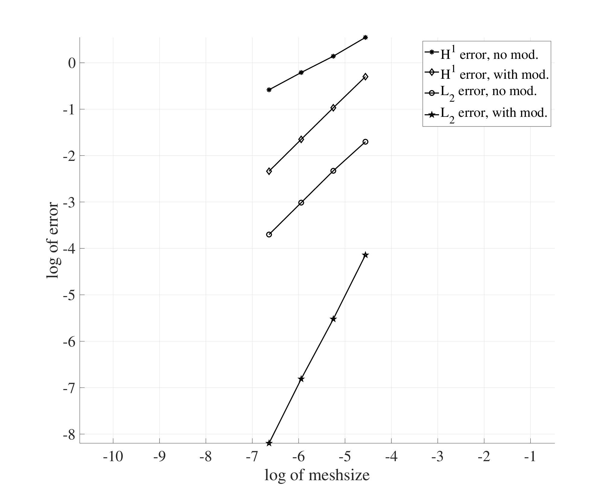
In Fig. 2 we show the convergence in $L_{2}(\Omega_{h})$ and $H^{1}(\Omega_{h})$ with and without boundary modification. In Fig. 3 we show the error in multiplier computed as $\|(-\bm{n}\cdot\nabla u)|_{\partial\Omega_{h}}-\lambda_{h}\|_{\partial\Omega_{h}}$ . Optimal order convergence is observed for the modified method, convergence $O(h^{3})$ in $L_{2}(\Omega_{h})$ and $O(h^{2})$ in $H^{1}(\Omega_{h})$ ; the multiplier error is approximately $O(h^{2})$ .

Third order elements.

Next we use continuous piecewise third order polynomials for the approximation of $u$ , and for the approximation of $\lambda$ we use piecewise quadratic polynomials, discontinous on each element edge on $\Gamma_{h}$ . In Fig. 4 we show the convergence in $L_{2}(\Omega_{h})$ and $H^{1}(\Omega_{h})$ with and without boundary modification. In Fig. 5 we show the error in multiplier computed as above. Optimal order convergence is again observed for the modified method, convergence $O(h^{4})$ in $L_{2}(\Omega_{h})$ and $O(h^{3})$ in $H^{1}(\Omega_{h})$ ; the multiplier error is approximately $O(h^{3})$ . Note that no improvement over $P^{2}$ approximations can be seen in the unmodified method due to the geometry error being dominant.

An unstable pairing of spaces.

We finally make the observation that our modification has a stabilising influence on the approximation. We try continuous $P^{2}$ approximations of $u$ and discontinuous $P^{2}$ approximations of $\lambda$ . In this case we get no convergence without the modification due to the violation of the inf–sup condition, whereas with modification we obtain the optimal convergence pattern in $u$ and a stable multiplier convergence given in Fig 6.

5.2 Rectangular elements

This example shows that it is possible to achieve optimal convergence even on a staircase boundary. We use a continuous piecewise $Q_{1}$ approximation on the (affine) rectangles, again enhanced for inf–sup, now by hierarchical $P^{2}$ bubble function on the boundary edges, together with edgewise constant multipliers on $\Gamma_{h}$ . We use the manufactured solution $u=\sin(x^{3})\cos(8y^{3})$ on the domain inside the ellipse $x^{2}/4+y^{2}=1$ . Our computational grids consist of elements completely inside this ellipse; a typical coarse grid is shown if Fig. 7 where we note the staircase boundary. In Fig. 8 we show elevations of the numerical solutions on a finer grid without and with boundary correction. In Fig. 9 we show the errors of the unmodified and modified methods. Again we observe optimal order convergence for the modified method, $O(h^{2})$ in $L_{2}(\Omega_{h})$ and $O(h)$ in $H^{1}(\Omega_{h})$ .

6 Concluding remarks

We have introduced a symmetric modification of the Lagrange multiplier approach to satisfying Dirichlet boundary conditions for Poisson’s equation. This novel approach allows for affine approximations of the boundary, and thus affine elements, up to polynomial approximation order 3 without loss of convergence rate as compared to higher order boundary fitted meshes. The modification is easy to implement and only requires that the distance to the exact boundary in the direction of the discrete normal can be easily computed. In fact, the modification stabilises the multiplier method so that unstable pairs of spaces can be used, as long as there is a uniform distance to the boundary.

Acknowledgement.

This research was supported in part by EPSRC, UK, Grant No.
EP/P01576X/1, the Swedish Foundation for Strategic Research Grant No. AM13-0029, the Swedish Research Council Grants No. 2013-4708, 2017-03911, 2018-05262, and Swedish strategic research programme eSSENCE.

References

[1] F. Ben Belgacem and Y. Maday. The mortar element method for three-dimensional finite elements. RAIRO Modél. Math. Anal. Numér., 31(2):289–302, 1997.
[2] T. Boiveau, E. Burman, S. Claus, and M. Larson. Fictitious domain method with boundary value correction using penalty-free Nitsche method. J. Numer. Math., 26(2):77–95, 2018.
[3] D. Braess and W. Dahmen. Stability estimates of the mortar finite element method for $3$ -dimensional problems. East-West J. Numer. Math., 6(4):249–263, 1998.
[4] J. H. Bramble, T. Dupont, and V. Thomée. Projection methods for Dirichlet’s problem in approximating polygonal domains with boundary-value corrections. Math. Comp., 26:869–879, 1972.
[5] E. Burman and P. Hansbo. Deriving robust unfitted finite element methods from augmented Lagrangian formulations. In S. P. A. Bordas, E. Burman, M. G. Larson, and M. A. Olshanskii, editors, Geometrically Unfitted Finite Element Methods and Applications, pages 1–24. Springer, Cham, 2017.
[6] E. Burman, P. Hansbo, and M. G. Larson. A cut finite element method with boundary value correction. Math. Comp., 87(310):633–657, 2018.
[7] E. Burman, P. Hansbo, and M. G. Larson. A cut finite element method with boundary value correction for the incompressible Stokes’ equations. In F. A. Radu, K. Kumar, I. Berre, J. M. Nordbotten, and I. S. Pop, editors, Numerical Mathematics and Advanced Applications ENUMATH 2017, pages 183–192. Springer, Cham, 2019.
[8] T. Dupont. ${L}_{2}$ error estimates for projection methods for parabolic equations in approximating domains. In C. de Boor, editor, Mathematical Aspects of Finite Elements in Partial Differential Equations, pages 313–352. Academic Press, New York, 1974.
[9] D. Gilbarg and N. S. Trudinger. Elliptic partial differential equations of second order. Classics in Mathematics. Springer-Verlag, Berlin, 2001. Reprint of the 1998 edition.
[10] A. Johansson and M. G. Larson. A high order discontinuous Galerkin Nitsche method for elliptic problems with fictitious boundary. Numer. Math., 123(4):607–628, 2013.
[11] C. Kim, R. D. Lazarov, J. E. Pasciak, and P. S. Vassilevski. Multiplier spaces for the mortar finite element method in three dimensions. SIAM J. Numer. Anal., 39(2):519–538, 2001.
[12] A. Main and G. Scovazzi. The shifted boundary method for embedded domain computations. Part I: Poisson and Stokes problems. J. Comput. Phys., 372:972–995, 2018.
[13] A. Main and G. Scovazzi. The shifted boundary method for embedded domain computations. Part II: Linear advection–diffusion and incompressible Navier–Stokes equations. J. Comput. Phys., 372:996–1026, 2018.

Refer to caption — Figure 1: Elevation of the discrete solution on triangles.

	$\displaystyle\|\mspace{-1mu}\|\mspace{-1mu}\|(u-u_{h},\tilde{\lambda}-\lambda_{h})\|\mspace{-1mu}\|\mspace{-1mu}\|$	$\displaystyle\lesssim h^{k}\\|u\\|_{H^{k+1}(\Omega)}+h^{-1/2}\delta_{h}^{2}\sup_{0\leq t\leq\delta_{0}}\\|D^{k+1}u\\|_{L^{2}(\partial\Omega_{t})}$		(3.18)
		$\displaystyle\qquad+{\color[rgb]{0,0,0}h^{1/2}}\delta_{h}^{l+1}\sup_{-\delta_{0}\leq t<0}\\|D_{n}^{l}(f+\Delta u)\\|_{L^{2}(\partial\Omega_{t})}.$

$\displaystyle\|\mspace{-1mu}\|\mspace{-1mu}\|(u-\tilde{u}_{h},0)\|\mspace{-1mu}\|\mspace{-1mu}\|$	$\displaystyle+\\|h^{\frac{1}{2}}\bm{n}_{h}\cdot\nabla(u-\tilde{u}_{h})\\|_{\partial\Omega_{h}}+\\|h^{-\frac{1}{2}}(\tilde{u}_{h}+\varrho\bm{n}_{h}\cdot\nabla\tilde{u}_{h}-\tilde{g})\\|_{\partial\Omega_{h}}$
	$\displaystyle\lesssim h^{k}\\|u\\|_{H^{k+1}(\Omega)}+h^{-1/2}\varrho_{h}^{2}\sup_{0\leq t\leq\delta_{0}}\\|D^{k+1}u\\|_{L^{2}(\partial\Omega_{t})}$	(3.19)
	$\displaystyle\qquad+{\color[rgb]{0,0,0}h^{1/2}}\varrho_{h}^{l+1}\sup_{-\delta_{0}\leq t<0}\\|D_{n}^{l}(f+\Delta u)\\|_{L^{2}(\partial\Omega_{t})}.$

	$\displaystyle\\|\pi_{k-1}\nabla\tilde{u}_{h}-\nabla\tilde{u}_{h}\\|_{\Omega_{h}}$	$\displaystyle\leq\\|\pi_{k-1}(\nabla\tilde{u}_{h}-\nabla u)\\|_{\Omega_{h}}+\\|\pi_{k-1}\nabla u-\nabla u\\|_{\Omega_{h}}+\\|\nabla u-\nabla\tilde{u}_{h}\\|_{\Omega_{h}}$		(3.32)
		$\displaystyle\leq\\|\pi_{k-1}\nabla u-\nabla u\\|_{\Omega_{h}}+2\\|\nabla u-\nabla\tilde{u}_{h}\\|_{\Omega_{h}}.$		(3.33)