EVOLUTION OF THE GAS MASS FRACTION OF PROGENITORS TO TODAY’S MASSIVE GALAXIES:
ALMA OBSERVATIONS IN THE CANDELS GOODS-S FIELDJournal: ApJ
Abstract
We present an ALMA survey of dust continuum emission in a sample of 70 galaxies in the redshift range selected from the CANDELS GOODS-S field. Multi-Epoch Abundance Matching (MEAM) is used to define potential progenitors of a galaxy of stellar mass . Gas masses are derived from the 850m luminosity. Ancillary data from the CANDELS GOODS-S survey are used to derive the gas mass fractions. The results at are mostly in accord with expectations: The detection rates are 75% for the redshift bin, 50% for the bin and 0% for . The average gas mass fraction for the detected galaxies is and for the sample. This agrees with expectations for galaxies on the star-forming main sequence, and shows that gas fractions have decreased at a roughly constant rate from to . Stacked images of the galaxies not detected with ALMA give upper limits to of and , for the and redshift bins. None of our galaxies in the and sample are detected and the upper limit from stacked images, corrected for low metallicity, is . We do not think that lower gas-phase metallicities can entirely explain the lower dust luminosities. We briefly consider the possibility of accretion of very low-metallicity gas to explain the absence of detectable dust emission in our galaxies at .
Keywords:
cosmology: observations — galaxies: formation — galaxies: high redshift – galaxies: photometry — galaxies: evolutionI Introduction
A fundamental process by which galaxies acquire mass is by accreting gas and converting it into stars. This process is especially important during the epoch extending from the reionization era to the peak of star formation activity at . The accretion process and how it is related to the star formation history of these early galaxies is, however, poorly understood from an observational point of view. We know that the gas accretion rate increases with increasing redshift, and at , it may exceed the star formation rate, leading to galaxies whose baryonic content are dominated by interstellar gas (e.g. Papovich et al. 2011). At lower redshifts, the star formation rate eventually exceeds the gas accretion rate, leading to a decreasing gas mass fraction. In addition to providing fuel for the star formation activity, the interstellar gas also fuels activity in the galactic nuclei. The star formation and AGN activities are coeval and follows the same strong evolution with redshift, showing a broad maximum around (e.g. Madau & Dickinson 2014). The gas mass fraction in massive galaxies in the local universe, like the Milky Way, is typically 10% and the star formation activity has fallen to a level last seen during the end of the reionization epoch at 7 (e.g. Madau & Dickinson 2014).
Despite the importance of gas accretion and the role of the interstellar gas during the formation of galaxies and their subsequent evolution, almost all of our knowledge about galaxies at high redshift is based on observations of stellar light. A tight correlation between star formation activity and stellar mass exists at the epoch of maximum star formation activity, and extends to earlier epochs (Daddi et al. 2007; Noeske et al. 2007; Magdis et al. 2010; Rodighiero et al. 2010, 2011). This correlation evolves smoothly with redshift (e.g. Madau & Dickinson 2014 and references therein) and is seen as an indication that the star formation history of most galaxies is driven by an interplay between gas accretion, star formation and feedback processes. Hence, observations of the stellar component only offers one piece of an intricate puzzle.
Our lack of knowledge about the interstellar medium (ISM) in high redshift galaxies stems from the difficulties associated with observing the gaseous component. Studies of the warm ionized gas through near-infrared spectroscopy of rest-frame optical lines provide some information, but in terms of mass this gas component only represents a small fraction of the total amount of interstellar gas. The cold and dense ISM, the most massive ISM component and the one directly involved in the formation of new stars, makes its presence known indirectly through extinction of rest-frame ultraviolet (UV) and optical light but is difficult to observe directly. In the local universe the atomic and molecular ISM components are usually studied using radio techniques. However, due to radio interference, the 21 cm HI line can only be observed in nearby galaxies. Observations of rotational lines of CO, tracing the more abundant molecular hydrogen, can be observed in high redshift galaxies (e.g. Carilli & Walter 2013; Combes 2018). While observation of CO in galaxies at the highest redshifts is possible, it has mainly been of highly special systems such as massive star forming submillimeter galaxies (SMGs; Capak et al. 2011; Walter et al. 2012; Riechers et al. 2013; Vieira et al. 2013; Zavala et al. 2018), and AGN host galaxies, the latter which has been observed at (Venemans 2012; 2017). A growing number of CO observations of main sequence star forming galaxies at redshifts are beginning to provide insights in the molecular ISM of more normal galaxies at high redshift (see Carilli & Walter 2013; Combes 2018), but these observations come at a high cost in telescope time, even with a facility like the Atacama Large Millimeter/submm Array (ALMA).
A faster, albeit less direct, method to estimate the gas mass in high redshift galaxies is to use a single flux density measurement of optically thin dust emission. This approach uses dust continuum emission as a proxy for the dense interstellar gas. The optically thin Rayleigh-Jeans part of the dust continuum emission is proportional to the dust mass, with only a linear dependence on the dust temperature (Scoville et al. 2014). The interstellar gas mass can then be derived if the gas-to-dust mass ratio is known. Scoville et al. (2014) derived an empirical relation between the specific luminosity of dust continuum emission at a wavelength of 850m and the gas mass determined through other means (mainly CO observations) for a sample of local Ultraluminous Far-Infrared Galaxies (ULIRGs) and massive star forming galaxies at . The ratio has a surprisingly small scatter and can thus be used to measure the interstellar gas mass from the dust continuum emission. This provides a fast and accurate method to derive the gas mass in distant galaxies at any redshift, and allows studies of the dense and cold interstellar gas at high redshift of statistically meaningful samples. A caveat with using the dust continuum emission, as well as the CO line, for measuring the gas mass, is its dependence on the gas-phase metallicity. This is not a problem for galaxies with close to solar metallicity, but the gas-to-dust mass ratio has a linear dependence on the metallicity (Draine et al. 2007) and care has to be exercised when observing galaxies of lower stellar mass, possibly with significantly lower than solar metallicity.
There have been several recent studies of the gas mass fraction in galaxies at high redshifts. Observations of CO line emission of galaxies at shows that the gas mass fraction is increasing dramatically compared with that found in the local universe (Daddi et al. 2010; Geach et al. 2011; Magnelli et al. 2012; Tacconi et al. 2013, 2018; Papovich et al. 2016; Freundlich et al. 2019). Using dust continuum emission as a proxy for the interstellar gas mass has allowed these studies to be pushed to (Scoville et al. 2014, 2016; Schinnerer et al. 2016), showing a further increase in the gas mass fraction. These results provide an overall picture of the growth of the gas mass fraction with look-back time which is largely consistent with expectations from theory. The samples, however, are selected using different criteria, and do not necessarily reflect an evolutionary scenario of the same galaxies seen at different epochs, making a comparison across cosmic time difficult.
Observations of dust continuum emission now extends to some of the highest redshifts. For instance, Tamura et al. (2018) report of thermal dust emission from a =8.31 galaxy. This galaxy, which is also detected in the [OIII] 88m fine-structure line, is gravitationally lensed by the foreground cluster MACS J0416.1-2403. The de-lensed dust mass is estimated to be M⊙ with a stellar mass of M⊙, showing that metal enhancement has occurred in some very young galaxies in the reionization epoch. It is, however, not yet possible to assess the gas mass fraction at these very high redshifts as no well-defined samples have yet been compiled.
As observations probe higher redshifts it becomes increasingly important to define samples that reflect the true evolution of galaxy properties. Galaxies need to be selected in a way that connects the properties of a given =0 galaxy, the descendant, with that of its high redshift progenitors, using already known characteristics of the galaxies such as stellar mass. Several studies have defined galaxy samples across different redshifts based on constant co-moving number densities (Papovich et al. 2011; Brammer et al. 2011; van Dokkum et al. 2013; Patel et al. 2013; Leja et al. 2013). This provide samples which are better suited for studies of how galaxy characteristics evolve with cosmic time, than a simple stellar mass cut-off or luminosity selection can do. Another method is to select galaxies at different redshifts based on their ranking, for instance, by selecting the most massive galaxies in equal co-moving volumes at different redshifts. Neither of these methods, however, fully account for the effects of galaxy evolution (e.g. Leja et al. 2013), basically by ignoring scatter and the stochasticity in the mass accretion history of the progenitors (Behroozi et al. 2013). An alternative selection strategy is to use abundance matching, or more precisely, Multi-Epoch Abundance Matching (MEAM; Moster et al. 2013; Behroozi et al. 2013). The MEAM method provides a parametrized relation between halo mass, as derived from numerical simulations, and stellar mass, based on observations of the stellar mass function, as a function of redshift. This method connects the growth of central dark matter halos with the growth and evolution of the stellar content and allows us to define the most likely progenitors of a given =0 galaxy while taking the stochastic nature of galaxy growth into account. While it does not account for all of the baryonic content of galaxies, only the stellar component, it does provide a recipe for selecting galaxies connected across cosmic time in an evolutionary sequence.
In this paper we present a study of the gas mass fraction in a sample of 70 galaxies selected using to the MEAM method (Sect. II.1) across the redshift range . The selection is based only on stellar mass and redshift and is completely unbiased with regards to luminosity, morphology or star formation activity. Our sample contains the most likely progenitors of a =0 galaxy of stellar mass . The gas mass is derived from optically thin dust continuum emission, using the conversion between 850m specific luminosity and interstellar gas mass derived by Scoville et al. (2014, 2016). We correct the observed fluxes for the effects of the Cosmic Microwave Background as well as discuss the impact of low gas-phase metallicity for the galaxies with the lowest stellar mass in our sample.
The paper is structured as follows: Sect. II presents the method used for defining the sample of galaxies and its application on the CANDELS GOODS-S data; Sect. III presents our ALMA observations, data reduction and the corresponding ancillary CANDELS data; Sect. IV presents our results; in Sect. V we discuss the results in more detail and explore the impact of a low gas-phase metallicity. Sect. VI presents a summary of our conclusions. For consistency with previous CANDELS publications we adopt the following cosmology: km s-1 Mpc-1, and .
II Sample Selection
II.1 The MEAM selection
A central theme with the study presented in this paper is to compare properties of galaxies at different redshifts, connected through an evolutionary sequence. To accomplish this we identify the likely high redshift progenitors of local galaxies of a given stellar mass using the Multi-Epoch Abundance Matching (MEAM) method. The resulting sample is thus selected based only on stellar mass and redshift, without considering other parameters. Such a sample is well suited for studying the evolution of properties such as, but not limited to, the gas mass fraction.
The method of abundance matching combines results from numerical dark matter simulations with observed properties of galaxies (Marinoni et al. 2002; Behroozi et al. 2010; Moster et al. 2010). In particular the multi-epoch abundance matching method developed by Behroozi et al. (2013) and Moster et al. (2013) provides an approach to determine the relationship between the stellar masses of galaxies and the masses of their host dark matter halos, while taking the stochastic nature of the merger process as well as observational uncertainties into account. Instead of attempting to model the complicated baryonic physics associated with star and galaxy formation, including feedback processes, the abundance matching methods populate dark matter halos, obtained from numerical simulations, with galaxies using a parametrized empirical model with adjustable parameters. The only observational input to these methods is the observed stellar mass function at a given redshift. The stellar-to-halo mass relation (SHM) can then be determined. The MEAM method assumes a functional form for the SHM relation (see Eq. 2 in Moster et al. 2013), populates the halos with galaxies and computes a model stellar mass function. The parameters of the SHM are then adjusted until the observed stellar mass function is reproduced. The redshift evolution of this relation is driven by gas infall, star formation, merging satellite galaxies and stellar mass loss.
Using the MEAM method we define a region in - space where progenitors of a z=0 galaxy of a given stellar mass are most likely to be located. We incorporate the statistical scatter in the merger tree from the Bolshoi simulation (Behroozi et al. 2013) and the relation derived from the Millennium simulation (Moster et al. 2013). The result is shown in Fig. 1, where the different slices correspond to five galaxies of different stellar masses at =0. The selection regions overlap at high redshift, representing the stochastic nature of the evolution of the merger trees for individual galaxies. From this selection we define progenitor galaxies to a =0 galaxy of , located at redshifts up to (shown as the purple area in Figure 1). In order to avoid selecting galaxies overlapping with lower mass =0 descendants, we sampled galaxies in the upper half of the purple area shown in Figure 1. It is worth noting that at all redshifts, the selected galaxies traces the upper branch of the stellar mass function and thus minimizes the overlap from galaxies with higher stellar masses. No selection criteria other than the stellar mass and redshift are used in defining the sample.
II.2 The CANDELS GOODS-S sample
The galaxies for our ALMA observations are taken from the CANDELS11 1 CANDELS: Cosmic Assembly Near-infrared Deep Extragalactic Legacy Survey; GOODS-S: Great Observatories Origin Deep Survey - South GOODS-S survey (Grogin et al. 2011; Koekemoer et al. 2011). We use the CANDELS GOODS-S H-band selected catalog, which contains 34,930 galaxies (Guo et al. 2013). All galaxies in the CANDELS catalog have photometric or spectroscopic redshifts. Stellar masses, and other properties have been derived using multiple spectral energy distribution (SED) models (e.g. Santini et al. 2015). See Section III.2 for additional details about the CANDELS data.
From this catalog we randomly select 70 galaxies in four redshift bins centered on z=2, 3, 4 and 522 2 More specifically: ; ; and .. The redshift bins are referred to as the =2, 3, 4 and 5 samples, respectively. In practice, the selection of galaxies constitutes a continuum from . The properties of the 70 galaxies in our sample are listed in Table 1 and Table 2. The selection is constrained by requiring the galaxies in each bin to have stellar masses within the limits defined through the MEAM method (Sect. II.1). This means that the selected galaxies are likely progenitors of a =0 galaxy of 11.2 (the purple region in Figure. 1). Each redshift bin contains 20 galaxies, except the =5 sample where we only have 10 galaxies. The reason for reducing the sample size for the highest redshift bin is two-fold. The MEAM method of Moster et al. (2013) and Behroozi et al. (2013) is defined up to , and hence, the extension to is an extrapolation and its validity decreases with increasing redshift. A second reason is that we are selecting progressively less massive galaxies at higher redshift and need to compensate with longer integrations to achieve a lower rms noise. As long as the observations probe the rest-frame Rayleigh-Jeans part of the dust SED, the negative K-correction ensures that the sensitivity for a given FIR luminosity is approximately constant with redshift (e.g. Blain & Longair 1996). However, for similar gas mass fractions, a galaxy with lower stellar mass also has a lower gas mass and, hence, a lower flux density than a galaxy with a larger stellar mass. The ratio of the average stellar mass of our =2 and =4 samples is 10. This is partially compensated by an increasing gas mass fraction. A gas mass fraction of 0.5 at =2 and 0.8 at =4 corresponds to an increase in by a factor of 4. We therefore need to achieve 40% lower rms noise for the galaxies compared to the galaxies.
We emphasize that our galaxy sample is only defined based on stellar mass and redshift. Hence, this sample is likely to represent an unbiased selection of the same population of galaxies, seen at different epochs, unlike a pure mass cut-off or luminosity selected sample.
III Data and Analysis
III.1 ALMA observations and data reduction
The ALMA observations of our sample were done during the Cycle 3 and 4 observing seasons. The =4 and =5 samples, targeting a total of 30 galaxies, were observed on April 30, 2016, using 41 12-m antennas. The =3 sample, targeting 20 galaxies, was observed during multiple sessions during the period June 18 - December 14, 2016, using 41-50 12-m antennas. Finally, the =2 sample, targeting 20 galaxies, was observed December 17-28, 2016, using 50 12-m antennas. The =4–5 observations were done using the Band 6 receivers, 230 GHz (1.3 mm), while the =2–3 observations were done using the Band 7 receivers, 345 GHz (870m). The choice of ALMA bands ensures that we observe the rest-frame dust continuum on the Rayleigh-Jeans part of the dust SED. The four redshift bins sample the SED at rest-frame and m, respectively. The correlator was configured to process a total bandwidth of 7.5 GHz, consisting of four 1.875 GHz-wide spectral windows. Each of the windows has 128 dual polarization channels. These channels were combined to produce the final continuum image.
The data consist of 70 individual observations, one for each of the targeted galaxies. Each of the four redshift intervals were packed into an scheduling block (SB) and executed until the required rms noise had been achieved. The bandpass calibrator for the =2 SB was the unresolved QSO J0522-3627, for =3 the QSO J023+1636 was used and for =4 and =5 J0334-4008 was used. Ceres and Pallas were primary flux calibrators. Phase calibrators were J0348-2749 and J0324-2918. The weather conditions varied during the observations but the overall phase solutions have smooth variations across each SB execution. The array configurations used during the observations were selected to give the requested angular resolution of about 0505. In fact, the reason for spreading out the observations over more than 6 months was to retain a uniform angular resolution, thereby achieving a uniform sensitivity for all the data sets. An interferometer measures a finite number of angular scales, resulting in a filtering of the spatial frequencies. The reconstructed image therefore contains emission from a relatively small range of angular scales; from the smallest angular scale, usually just called the angular resolution, to the largest angular scale. Smooth emission on scales larger than the largest angular scale will be filtered out. Hence, retaining a uniform angular resolution safeguards against losing emission due to these effects33 3 See Observing with ALMA – A Primer: https://almascience.nrao.edu/documents-and-tools/cycle6/alma-science-primer.
The data were calibrated and reduced using the standard ALMA pipeline. The data was of good quality and met the required angular resolution of approximately 0505. The required 1 rms noise was set to 100Jy for the =2 and =3 B6 observations. For the =4 and =5 samples, the B6 rms noise requirements were 50Jy and 30Jy, respectively (see Sect. II.2). All the requirements were met with the ALMA data and are listed in Table 3. The center wavelengths of the continuum data for the B6 and B7 observations are 1,287m and 873m, respectively. We will refer to these as the 1.3mm and 870m data, or B6 and B7 data, in the rest of this paper. The full half-power beam width (HPBW) of the ALMA 12-m antennas, our instantaneous field of view, is 265 for the B6 data and 180 for the B7 data. The combined area within the HPBW of all 70 ALMA pointings is 7.4 arcmin2. Several off-center submm sources were detected and will be discussed in a separate paper.
Continuum images of the 70 ALMA pointings were produced using the CASA44 4 Common Astronomical Software Application task CLEAN. The data were naturally weighted for maximum sensitivity. In the natural weighting scheme, data are weighted relative to the number of angular scales observed. It provides the highest sensitivity, but does not maximize the angular resolution. For the latter, a uniform weighting can be used. It is also possible to combine natural and uniform weighting, so called Briggs weighting (Briggs 1995). We tried different weighting schemes in the CLEAN process to find the best trade-off between sensitivity and angular resolution. However, since almost all of the submm detected sources remain unresolved at the nominal 05 angular resolution, we did the final flux measurements using natural weights. The average observational properties of the four redshifts bin are given in Table 3. The positional accuracy of the peak of the submm emission is 01. In the CLEAN process we pixelated the image with a pixel size 0101. The actual resolution of the interferometer data, however, is larger than this. For example, the =3 galaxies have an average restoring beam of 056040, with a position angle of . Since the units of the continuum image is Jy/beam, the peak intensity corresponds to the integrated flux for completely unresolved sources. In almost all cases, however, the derived size of the submm emission is slightly larger than the restoring beam. This shows that while the emission is not resolved, it has an extent which is non-negligible in comparison with the angular resolution of the ALMA data. In these cases we derived the integrated flux by fitting a two-dimensional Gaussian to the emission. Of the detected galaxies, we found only one case where the peak flux was larger than the integrated flux. This corresponds to a case where the submm emission originates in two separate regions, each of them unresolved by the ALMA data. In this case we used the sum of the peak fluxes of the two components when deriving the gas mass.
As we target individual galaxies, the identification of detected sources is easier than in a blind survey. Nevertheless, in order to avoid false detections we set a detection limit of 5 for a source to be considered securely detected. Of the 26 detected galaxies (see Sect. IV) all but two are detected at more than 5. The two marginally detected sources (CANDELS ID: 2344 and 8433) are detected at 3.4 and 4.8 sigma, respectively. The latter is close to our 5 limit and included among our detected galaxies. Close inspection of the CANDELS ID 2344 shows that the submm emission is associated with a highly inclined star forming galaxy. We therefore treat this as a detection as well.
III.2 CANDELS data
Our sample was defined using CANDELS data from the GOODS-S field (Giavalisco et al. 2004; Grogin et al. 2011; Koekemoer et al. 2011). The redshifts and stellar masses initially used to define the sample came from the Wiki-Z method (e.g. Wiklind et al. 2014) applied to the CANDELS GOODS-S data. For the analysis presented here we use the official CANDELS catalogs, where photometric redshifts and stellar masses are compiled using several different teams applying different SED methods (Guo et al. 2013; Santini et al. 2015). Spectroscopic redshifts are used whenever reliable data are available. Thirteen of the galaxies galaxies in our sample have spectroscopic redshifts. The differences between the initial selection and the final catalog values are very small and do not affect the the sample selection or the results presented in this paper.
The CANDELS GOODS-S catalog contains 34,930 H-band selected sources, covering a total of 170 arcmin2. The multiwavelength catalog includes 18 bands and combines observations from the ERS/WFC3 and CANDELS/WFC3 data in the F098M, F105W, F125W, F140W and F160W filters. It includes UV data from both CTIO/MOSAIC and VLT/VIMOS, as well as optical GOODS-S and CANDELS data in the F435W, F606W, F775W, F814W and F850LP filters. Infrared data from VLT/HAWK-I Ks (Fontana et al. 2014) and Spitzer/IRAC 3.6, 4.5, 5.8 and 8.0m (Ashby et al. 2013) are also part of the data set. See Guo et al. (2013) for a summary of the CANDELS GOODS-S UV-to-mid-IR data set and corresponding survey references. The redshifts and stellar mass estimates used in our analysis are from Santini et al. (2015). In addition to redshift and stellar mass, all of the galaxies in the CANDELS GOODS-S catalog have estimates of the extinction, age, star formation history and metallicity (see Table 2). These estimates will be used to characterize the galaxies in our sample. We also use data on the size and morphology of the galaxies in the CANDELS GOODS-S catalog from van der Wel et al. 2012. The size estimates are derived using Sextractor and the morphological classification relies on the one-dimensional Sérsic index derived using the WFC3/F160W data. Given the redshift range of our sample, the Sérsic index is derived at rest-frame wavelengths ranging from 5100Å for our =2 galaxies, to 2700Å for the =5 galaxies.
In order to improve the results from the CANDELS survey, a team effort to analyze methods used to derive galaxy properties, such as photometric redshift, stellar mass and other parameters characterizing the galaxy population, was conducted. Photometric redshift estimates by eleven teams were presented in Dahlen et al. (2013). It was demonstrated that combining the photometric redshifts from multiple methods reduces the scatter as well as the outlier fraction in photometric redshift values. A comprehensive study comparing stellar mass estimates of both real galaxies and mock galaxies drawn from semi-analytical models, was presented in Mobasher et al. (2015). Here, the results of 10 teams showed that the biases are relatively small and mostly present for young galaxies with ages 100 Myr. In a similar manner, Santini et al. (2015) analyzed the results from 10 different teams fitting SEDs to the CANDELS GOODS-S and UDS data (Guo et al. 2013; Galametz et al. 2013). The resulting stellar mass catalog represents the CANDELS public release for the GOODS-S55 5 Catalogs for GOODS-S are available at http://candels.ucolick.org/data_access/GOODS-S.html and UDS66 6 Catalogs for UDS are available at http://candels.ucolick.org/data_access/UDS.html fields (Santini et al. 2015). We adopt the CANDELS GOODS-S public catalog for the redshift and stellar mass values of CANDELS GOODS-S galaxies used in this paper. Stellar masses are based on a Chabrier IMF. The public releases also contain the results from each of the participating teams of other parameters obtained from the SED fits. For these parameters we use median values for dust extinction, , metallicity, star formation rate (SFR) and specific star formation rate (sSFR). The CANDELS derived parameter values for the galaxies in our sample are listed in Table 2, together with average values for the different redshift bins.
IV Results
IV.1 Submm data
The data obtained with our ALMA observations are listed in Table 1. We detect submm emission in 15 out of 20 galaxies in the =2 sample, 11 out of 20 in the =3 sample and none in the =4 and =5 samples, with 20 and 10 galaxies observed, respectively. When detected, the submm emission is in almost all cases observed at 5, while for the non-detected sources, there is no hint of emission. We construct stacked ALMA images of the non-detected galaxies for each redshift bin. The number of galaxies in each stack is 5, 9, 20 and 10 for the =2–5 samples, respectively. The rms noise for the stacked =4 and 5 samples is 8Jy and 35Jy for the =2 and 3 samples (see Table 4). No submm emission was detected in any of the stacked images. For the =3–5 samples we randomly picked sub-samples of four galaxies and stacked the submm images. None showed any emission even at the 2 level. We use the upper limits of submm emission in the stacked images to set upper limits to the gas mass fraction.
Conversion of the submm fluxes into estimates of the total molecular gas mass is done using a single flux density measurement of the dust continuum on the Rayleigh-Jeans part of the dust SED. We use the empirical correlation between the rest-frame 850m luminosity, , and the total molecular gas mass, , derived by Scoville et al. (2014, 2016):
| (1) |
This correlation was obtained using local and high redshift galaxies with known submm luminosities and known molecular gas masses. The relation has an approximately linear dependance on dust temperature such that an increase in the dust temperature results in a smaller gas mass for a fixed flux density. The method was tested on local galaxies with approximately solar metallicity (e.g. Scoville et al. 2014; Groves et al. 2015), and for high redshift galaxies (Scoville et al. 2016). The high redshift galaxies were selected to have high stellar masses and should therefore have close to solar metallicity (Savaglio et al. 2005; Erb et al. 2006).
This approach has recently been explored using high-resolution cosmological simulations from the Feedback in Realistic Environment (FIRE) project (Hopkins et al. 2014; Liang et al. 2018). The simulations include galaxies at redshifts =2-4, with M⊙, exhibiting various forms of stellar feedback, and use radiative transfer modeling to estimate the FIR luminosity. The results show a tight correlation between the rest-frame luminosity and molecular gas mass for a wide range of star formation activity (Liang et al. 2018). This shows that the empirical approach of using a single flux density measurement to estimate the interstellar gas mass is viable. Nevertheless, one concern for our sample is that we target galaxies with stellar masses decreasing with increasing redshift and hence galaxies in our highest redshift bins may have a different conversion factor between and total gas mass than their lower redshift counterparts. We will discuss this in more detail in Section V. The gas mass of each galaxy is derived using the conversion factor as defined in Eq. 1, assuming a dust temperature K and dust emissivity index to derive (e.g. Scoville et al. 2016). A dust temperature of 25 K is likely to characterize the bulk of the dust mass. The median dust temperature of the dust in our Milky Way galaxy is 18 K (e.g. Planck Collaboration 2011). Dunne et al. (2011) found that typical dust temperatures for 1867 galaxies in the Herschel-ATLAS survey are in the range 17-30 K.
The observed submm fluxes at high redshifts need to be corrected for the effects of an increasing temperature of the Cosmic Microwave Background (CMB); see da Cunha et al. (2013) for a discussion and quantification of this correction. The CMB affects the observed fluxes by providing an additional heating source for the dust grains as well as an increasingly bright background against which the continuum emission is measured. These two effects compete against each other, but the net result is that the observed flux density needs to be corrected by a factor 1. The correction factor depends on the dust temperature, the observed wavelength and the redshift. For typical galactic dust temperatures, the correction becomes significant already at . The correction factors used here are listed in Table 1, for an assumed dust temperature of 25 K. The correction increases the flux density values, and hence the estimated gas mass, by 6% at and by 30% at . Due to the definition of the gas mass fraction used here, the effect on is of a lesser magnitude. For equal stellar and ISM masses, the CMB correction increases by 13% at and 2% at . All the results quoted in this paper and listed in Table 1 have been corrected for the CMB temperature at the corresponding redshifts.
IV.2 Gas mass fraction
The gas mass fraction is defined as . Upper limits to and the gas mass fraction correspond to 3 limits of the flux density. The stellar mass is obtained from the CANDELS GOODS-S data (Santini et al. 2015; see also Mobasher et al. 2015).
In Figure 2 we plot the gas mass fraction, , as a function of redshift. For the =2-3 redshift bins we plot both detected galaxies and 3 upper limits of undetected galaxies, as well as the average gas fraction for detected galaxies in the =2 (), and the =3 () redshift bins (the errors represent the dispersion of the mean). These values are significantly higher than the typical gas mass fraction in large spiral galaxies in the local universe of 0.1. The corresponding ISM gas masses range from M⊙, with an average of of M⊙ for the =2 sample, and M⊙ for the =3 sample. In Figure 2 we also show the 3 upper limits of the gas mass fraction for the stacked images of non-detected galaxies in each redshift bin (purple arrows). The expected gas mass fraction from three different scaling relations are also shown in Figure 2 (Sargent et al. 2014; Scoville et al. 2017; Tacconi et al. 2018). The scaling relations have been used to calculate the expected gas mass fraction for galaxies on the main sequence (MS) with a stellar mass, , corresponding to the average of the MEAM selection used for our sample (Sect. II.1, Figure 1). Overall, the measured values of the detected galaxies exhibit the expected increase with redshift for the =2 and =3 samples. The stacked upper limits (3 limits) on the other hand, deviate significantly from the scaling laws applicable for galaxies on the main sequence.
At any given redshift, our selection of galaxies is based on the galaxy stellar mass with a dispersion given by the MEAM models (Sect. II.1; Figure 1). We therefore derive the for each of the 26 galaxies with detected submm emission where we use the actual stellar masses, star formation rates and, in the case of the Tacconi et al. (2018) scaling relations, the effective radius, to calculate . The result is shown in Figure 3. The average for the Sargent et al. (2014) and Tacconi et al. (2018) scaling laws are and , respectively, showing an overall good correspondence between the observed and expected gas mass fractions for the galaxies with detected submm emission.
The fraction of galaxies with quenched star formation decreases with increasing redshift, as well as with decreasing stellar mass. One would therefore expect that the fraction of galaxies in our sample with detectable submm emission increases with redshift. This is not the case and instead our detection rate decreases from 75% at =2, to 50% at =3 and 0% for . Could this be due to a lack of sensitivity in our ALMA data or due to the random selection of galaxies within each redshift bin and a modest sample size?
Quiescent and star forming galaxies occupy distinct regions of the rest-frame versus color space (e.g. Williams et al. 2009). While all of the submm detected galaxies in our =2 and =3 samples have colors defining them as star forming, 3 out of the 5 undetected galaxies in the =2, and 5 out of the 9 undetected galaxies in the =3 sample, have colors implying they are quiescent. Incidentally, none of the galaxies in our bins fall in the quiescent region, but the color scheme is not well defined for these high redshifts. The regions in color space defining ‘quiescent’ and ‘star forming’ galaxies are binary in nature, although it does appear to distinguish between disk-like and spheroidal morphological types for (Patel et al. 2012). A more nuanced view of the star forming activity can be obtained through the extensive CANDELS photometry and corresponding SED fits. In particular, the SFR and stellar mass estimates allow us to define the sSFR. In Figure 4 we plot sSFR versus stellar mass for galaxies in each of our four redshift bins. Each bin contains all CANDELS GOODS-S galaxies, for that particular redshift interval. We mark those galaxies that fall within our MEAM selection limits, as well as the galaxies observed with ALMA. The main sequence sSFR for each redshift bin, and its 0.5 dex values, are marked (from Schreiber et al. 2015). From the figure it is clear that 2 out of 5 undetected galaxies in the sample have sSFR values 0.5-0.7 dex below the main sequence, and 6 out of 9 undetected galaxies in the sample have sSFRs 0.5-0.8 dex below the main sequence. These galaxies corresponds to the ‘quiescent’ galaxies in the color definition. We also note that the both the =2 and =3 redshift bins have undetected galaxies with sSFRs corresponding to galaxies on the MS as well as 0.5 dex above the MS. From Figure 4 it is clear that there are galaxies within our MEAM selection regions with sSFR values 0.1-0.3% of the corresponding MS value. These are likely to be truly quiescent galaxies, but none of these are part of our ALMA sample77 7 This is by pure chance as we selected galaxies randomly within each MEAM selection region..
The galaxies in the Tacconi et al. (2018) sample (cf. Freundlich et al. 2019), are selected based on their SFR and M∗ properties, i.e. their sSFR, aiming for a homogeneous coverage of the M∗–SFR plane above a certain stellar mass. Some of these galaxies do lie in the quiescent part of the UVJ diagram, despite being relatively close to the MS. The Tacconi et al. (2018) scaling relations are defined for stellar masses in the range and across . All of the galaxies in our sample falls within this mass range, and all of the inferred sSFRs are within and dex of the MS. Hence, the Tacconi et al’s scaling relations is applicable to our sample. For the undetected and galaxies, the scaling law predicts and , respectively. This is lower than for the detected galaxies but still higher than the upper limits derived from the stacked images ( and ). This will be discussed further in Sect V.2.
The SFRs used here are obtained from the multi-team SED fitting of the CANDELS data (Santini et al. 2015) and listed in Table 2. In order to determine whether our ALMA data is sensitive enough to detect these lower gas mass fractions, we need to relate the SFR to an expected observed submm flux density. We can convert the SFRs into FIR luminosities using the Kennicutt (1998) relation. Fitting a dust SED to our ALMA data using a modified black-body curve allows us to use the 3 noise rms to obtain lower limits to the detectable SFR. However, the FIR luminosity derived from the modified blackbody SED has a strong dust temperature dependence, as well as weaker dependencies on the dust emissivity index and the critical wavelength distinguishing between optically thick and thin emission (e.g. Scoville et al. 2014 and references therein). The dust emission therefore needs to be well-sampled by observations in order to provide a useful estimate of and corresponding SFR. This is not the case for our sample. We can, however, obtain a rough estimate of the minimum SFR that would result in detectable submm emission for a given rms noise level by using a modified blackbody SED and vary the dust temperature and other parameters within reasonable limits. Integrating the resulting SED gives the corresponding to our 3 detection limit. We vary the dust temperature between 25-35 K, the dust emissivity index and the critical wavelength m. This results in a lower limit to the SFR for individual galaxies in the range 4 M⊙ yr-1 ( K, ) to 14 M⊙ yr-1 ( K, ). Lower SFR values are obtained for the lower values of the dust temperature. With all parameters fixed, the lowest SFR values are obtained for the highest redshift bins due to the lower rms noise levels of the ALMA data. Assuming a dust temperature of 35 K, the SFR limits are between 9-14 M⊙ yr-1. Using the 3 rms noise from the stacked images we find that a star formation rate of 1-2 M⊙ yr-1 should have resulted in detectable submm emission. The latter limit assumes K. For a lower dust temperature, the limiting SFR decreases even further.
Hence, even in the case of a high dust temperature, K, all of the =2 galaxies and all except three =3 galaxies ought to have been detected in our ALMA data. The fact that 35% of the =2-3 galaxies were not detected means that they either lack the star formation required to power the dust emission and/or or have low dust content and gas-phase metallicities. For the =4 and =5 galaxies, almost half of the individual galaxies could remain undetected in our ALMA data if the dust temperature is as high as 35 K, but the other half should have produced detectable submm emission. If the dust temperature is 25 K we should have detected all except 3-4 galaxies in the =4–5 samples.
The SFR limits for the stacked galaxies without detected submm emission are in the range 1-2 M⊙ yr-1, for K. The fact that none of them show any hint of submm emission shows that these galaxies either have very low levels of star formation or a low gas-phase metallicity making the dust signature faint enough to evade detection. We will discuss this further in Sect. V.
IV.3 Comparison with CANDELS data
The availability of CANDELS data for all galaxies in our sample makes it possible to compare the derived gas mass fractions with characteristics of the galaxies derived from SED fits, such as morphology (characterized through the one-dimensional Sérsic index), the global dust extinction (), stellar metallicity and effective radius, among others. These parameters are derived using SED fits to the UV-to-NIR photometric data using different fitting algorithms, stellar isochrones, parametrization of the star formation history (SFH) and the inclusion, or omission, of nebular lines. In order to study, and account for, the impact of these effects, the release of CANDELS catalogs involved the effort of several teams within the CANDELS collaboration (e.g. Mobasher et al. 2015; Santini et al. 2015).
If the non-detected galaxies are quiescent systems, we expect them to have high Sérsic indices, low values as well as low SFR and sSFR values. These expectations are, for the most part, realized, as shown in Figures 5-7. In these figures we plot vs. Sérsic index, effective radius (), SFR, sSFR, extinction () and stellar metallicity. Individual results are shown for the detected =2 and =3 galaxies and for the corresponding averages. For the undetected galaxies, we show the 3 upper limit to from the stacked images versus averages for the different parameters.
In Figure 5 we plot the gas mass fraction, , versus the Sérsic index (left panel) and the effective radius, , in kpc (right panel). The =2 and =3 samples show a clear trend with the detected galaxies having a Sérsic index indicating a disk-like morphology, while the undetected galaxies, on average, have a more spheroidal morphology. The =4 and 5 samples fall in between the detected and undetected =2 and 3 samples. However, the uncertainty of the Sérsic indices for these high redshift galaxies is substantial. The right panel of Figure 5 shows that the submm detected galaxies are, on average, a factor two larger than the non-detected galaxies. The dispersion in is quite large but our results for =2-3 are consistent with the results of other studies (e.g. van Dokkum et al. 2008), where the effective radius for quiescent galaxies at 2 is 0.9 kpc. Star forming galaxies are typically 3 times larger (e.g. Straatman et al. 2015).
In Figure 6, we compare with the SFR and sSFR. In this case we use median values as each redshift bin shows a spread in SFR properties (see Table 2). Not surprisingly, the galaxies without detectable submm emission tend to have lower SFRs than those with detectable FIR emission. However, the median SFR of the undetected =2 sample is still 50 M⊙ yr-1, while the median SFR for the =2 and 3 samples with submm emission is 100 M⊙ yr-1. The =4 and 5 samples have the lowest SFRs, with values 10-15 M⊙ yr-1. However, the =4 and 5 samples show a very different behavior for the star formation rate per unit stellar mass (sSFR). In this case, the =4 and 5 galaxies have a normal sSFR (right panel in Figure 6), while the nondetected =2 and 3 galaxies have low sSFR values. The submm detected galaxies have median sSFR that would put them close to the main sequence at their respective redshifts. This can also be seen in Figure 4.
Finally, in Figure 7 we compare the gas mass fraction with dust extinction, characterized through , and the stellar metallicity (). Not surprisingly, the galaxies with detectable submm emission have higher extinction values than the undetected galaxies. The lowest extinction values are found for galaxies in the =4 and =5 redshift bins. Again, this is not surprising since our sample is drawn from an H-band selected catalog. At , the H-band samples rest-frame UV wavelengths of Å. Hence, the H-band selection has an intrinsic bias against dust obscured galaxies at these high redshifts. This will be discussed in Sect. V. There is a clear trend with high gas mass fraction galaxies in the =2 and 3 samples having a higher metallicity than those of the undetected galaxies, with an average metallicity . A somewhat surprising result is that the average metallicity of the galaxies in the =4–5 redshift bins have a metallicity close to solar, Z⊙. The metallicity of each galaxy is derived from SED fits and thus represent the metallicity of the stellar component, not the gas-phase metallicity. The metallicity derived from SED fits are subject to a degeneracy with stellar age and dust extinction. Hence, the metallicity derived for a single galaxy is not very accurate, but as an average of a larger sample, the SED based stellar metallicities are indicative of a trend (see Sec. V.3).
Randomly selected galaxies from the =2 and =3 samples are shown in Figure 8. For each redshift bin we show 5 submm detected and 5 non-detected galaxies. The morphological difference between the detected and non-detected galaxies in the =2 sample, also seen in their Sérsic indices, is obvious, but it is less evident in the =3 sample. In Figure 9 we show 5 randomly selected galaxies each for the =4 and the =5 samples. These galaxies are less massive and less luminous, which, combined with the surface dimming, makes their appearance at rest-frame UV and optical wavelengths more difficult to characterize. For each galaxy we show 7070 cut-outs in the ACS/F606W, ACS/F850LP, WFC3/F160W and VLT/HAWKI 2.2m filters, as well as the ALMA continuum image. The stretch of the ALMA continuum images are different in each case. The galaxy CANDELS ID #17427 appears to have a weak and extended emission feature associated with the target galaxy. However, the SNR is 2 and we do not treat this as a detection. CANDELS ID #6780 (a non-detected galaxy) has a neighbor with dust continuum but at a photometric redshift of =1.550 and therefore not physically related to the target galaxy and not part of our sample.
V Discussion
V.1 The gas mass fraction over cosmic time
In Figure 10 we compare our results of the gas mass fraction with results compiled from the literature. The estimates are derived from both CO J=1-0 through J=3-2 line observations (Geach et al. 2011; Daddi et al. 2010; Magnelli et al. 2012; Tacconi et al. 2013, 2018; Papovich et al. 2016; Freundlich et al. 2019) and from dust continuum emission (Scoville et al. 2016; Schinnerer et al. 2016; Tacconi et al. 2018; this paper). We have included data from the PHIBSS2 survey (Tacconi et al. 2018), containing gas mass estimates from both CO line and dust continuum for 1444 star forming galaxies at redshifts . Here we include galaxies up to . We also include CO data from Freundlich et al. (2019), covering the redshift range . The estimates of the gas mass fraction presented in Figure 10 are based on galaxies selected using different criteria, mainly stellar mass and star formation activity, and do not necessarily constitute an evolutionary sequence in the same sense as our selection is meant to do. However, all the observations at select relatively massive galaxies, and it is only for the highest redshifts that our sample selection differ by targeting lower mass galaxies. The errors shown in Figure 10 are dispersion of the mean and do not reflect uncertainties associated with the different estimates of mass, conversion factors or other possible systematic effects.
Schinnerer et al. (2016) selected a sample of massive, star forming galaxies in the COSMOS field with redshifts and found an average , which is identical to the gas mass fraction derived from our =3 sample, . The stellar masses of the galaxies making up the Schinnerer et al. (2016) sample is almost the same as for our =3 sample, and , respectively. Scoville et al. (2016) used dust continuum emission to estimate the gas mass fraction in three redshift bins, 1.2, 2.3 and 4.4. Their result for gives for galaxies with an average stellar mass . Our result for the =2 sample suggests a higher gas mass fraction at this redshift, with , for galaxies that on average are 1.7 times less massive. Tacconi et al. (2013) used the CO, J=3-2 emission line to estimate the gas mass fraction in a sample of galaxies at =2.2. Using a Galactic value for the CO-to-H2 conversion factor they derive an average gas mass fraction of 0.47. The average stellar mass of their sample of .
Figure 10 clearly shows that the gas mass fraction increases dramatically with redshift. The curve shown in the figure depicts the expected gas mass fraction from the scaling relation of Sargent et al. (2014) for galaxy stellar masses following our selection method. The data shows a steeper increase in the gas mass fraction for than indicated by the scaling relation. The scaling relation from Scoville et al. (2018) depicts a steeper rise in the gas mass fraction for this redshift range, but still falls below the observed values for (see Figure 2). The scaling laws used here are based on MS galaxies with stellar masses given by our MEAM selection and do not take individual star formation parameters into account.
If we plot the observed gas mass fractions as a function of cosmic time rather than redshift, they can be fitted by a linear relation: . The fit is made over the range =3 to =0 and include all the corresponding data points shown in Figure 10. This result shows that the gas mass fraction for galaxies in the mass range , on average, decreases at a constant rate of Gyr-1 over a time interval of 11.5 Gyr. The fit is shown, as a function of redshift, in the right panel of Figure 10 (thick black line).
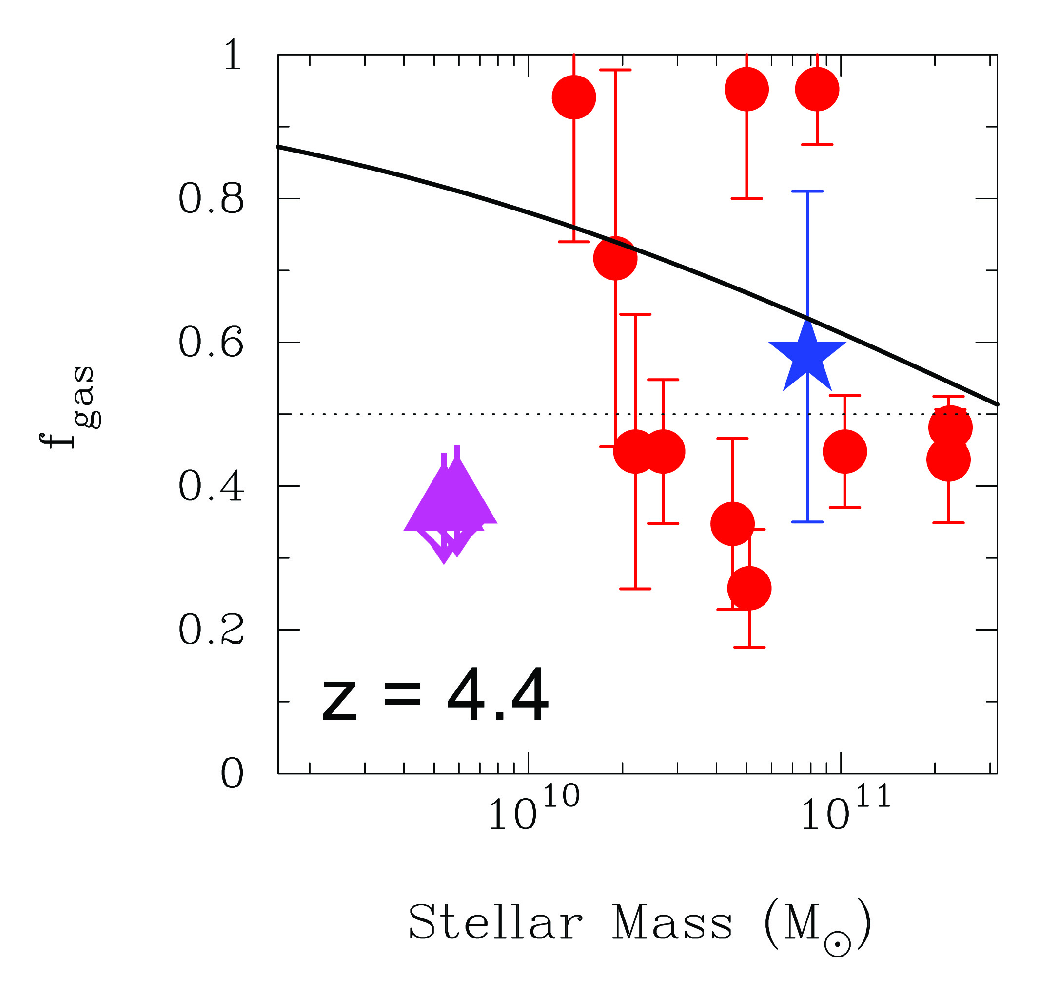
Galaxies with a larger stellar mass are believed to have a lower gas mass fraction. The observed down-turn in the gas mass fraction for 4, as seen in Figure 10, is therefore most likely attributed to the fact that the sample of Scoville et al. (2016) contains galaxies that have an average stellar mass 15 times higher than those for which the scaling laws shown in Figure 10 are based. This is illustrated in Figure 11 were we plot the expected gas mass fraction as a function of stellar mass for a fixed redshift of =4.4. In fact, a tendency for this is seen in the Scoville et al. (2016) data as it covers a range of stellar masses. The same trend is also reflected in the scaling relations (Sargent et al. 2014; Scoville et al. 2017; Tacconi et al. 2018).
Hence, several studies, using both dust continuum emission and CO line emission as estimates of the interstellar gas mass, agree that the gas mass fraction at redshifts and are 0.5 and 0.6, respectively. There may be a dependence on the galaxy stellar mass in the sense that for a given redshift, less massive galaxies have a higher gas mass fraction than more massive ones. These gas mass fractions should be compared with the situation in the local universe, where massive galaxies, like our Milky Way, typically have , while dwarf galaxies can have much higher gas mass fractions (e.g. Schombert et al. 2001; Bergum et al. 2008). Taking the disparity of the sample selection into account, as well as the disparity in the techniques used to infer the interstellar gas masses and the associated potential systematic effects and biases, the consistency in the dramatic rise of the gas mass fraction with redshift is quite remarkable and reflects the profound importance that the interstellar gas has on regulating the star formation history of galaxies as they evolve with cosmic time. Adopting a fiducial gas mass fraction of 0.08 at =0, these results show that the gas mass fraction grows as over , and even steeper if we only consider the redshift range.
V.2 Non-detections of dust continuum from stacked images
One intriguing aspect of the gas mass fraction estimates for galaxies in our sample is the result for stacked images of galaxies without detectable dust continuum emission. In Figure 2 these upper limits are marked by purple arrows and represent upper limits to the gas fraction with a 3 upper limit of the gas mass. In Figure 10 the =4 and =5 upper limits are marked as red arrows. These limits are significantly lower than the gas fractions of the detected galaxies at =2-3 as well as the expected gas mass fraction derived from scaling laws. The upper limits to the gas fractions are listed in Table 4.
As discussed in Sect IV.2, about half of the non-detected galaxies at and have sSFRs lower than those that are submm detected (Figure 4). The sSFR of the non-detected galaxies are within a factor 0.8 dex of the sSFR of main sequence at the corresponding redshift and stellar mass range. Hence, these galaxies are not completely devoid of star formation activity, and in Sect. IV.2 we showed that the expected gas mass fraction, taking their lower sSFR values into account, is higher than the upper limits obtained from the stacked images. It thus appears that the effect of a relatively modest reduction in the specific star formation rate has a large effect on the dust emission. It is not clear whether these galaxies are transitioning to a truly quiescent stage, or if they are in a low-activity phase of episodic star formation activity. The high average Sérsic index of the non-detected and galaxies (Figure 5) could suggest that they are transitioning to become a part of the truly quiescent population.
None of our galaxies in the and samples are detected with ALMA and the upper limits to the gas mass fractions derived from stacked images (0.38 and 0.37, respectively) are much lower than what is expected from scaling relations. They are, however, not dead galaxies in terms of their star formation activity, as seen through their SFRs. Their average star formation rate per unit stellar mass shows that they are as efficient in forming stars as their lower redshift counterparts (Figure 4 and 6). The difference is that the galaxies have stellar masses 10 times lower than the =2 sample. Defining the star formation efficiency (SFE) as in units of Gyr-1, we find that the submm detected galaxies have , while the =4 and 5 samples have . The undetected =2 and 3 galaxies have . Since stars are formed from interstellar gas, this suggests that either the star formation process is 2-4 times more efficient at , using up the interstellar gas faster than it can be replenished, or the total amount of interstellar gas in galaxies is not reflected in the dust continuum, at least not in the stellar mass ranges probed in this study. The inverse of the SFE is the gas depletion time scale, corresponding to Gyr and Gyr for the submm detected galaxies and galaxies, respectively.
As discussed in Sect. IV, there is an intrinsic bias against finding dust-obscured galaxies at using optical and near-infrared selected catalogs. This certainly applies to the CANDELS GOODS-S catalog which is based on H-band selected sources. At the H-band corresponds to rest-frame UV wavelengths and the presence of dust obscuration in low-mass galaxies at these redshifts, with corresponding low luminosities, may simply make them too faint to be included in the catalog. Such galaxies should show up in blind submm surveys as submm emission with no obvious optical/NIR counterpart. However, the fact that only a single galaxy was found in the 4.5 armin2 ALMA continuum survey of the Hubble Ultra Deep Field (HUDF; Dunlop et al. 2017), none in the very deep 1.6 arcmin2 survey of the HUDF (Aravena et al. 2016), and none in an ALMA survey of three of the Frontier Fields (Laporte et al. 2017), argues against a ‘hidden population’ of dusty, far-infrared luminous, star forming low-mass galaxies at high redshift. The single exception in the UDF is CANDELS ID 12781 (Dunlop et al. 2017), which is a faint galaxy with a photometric redshift and M⊙.
V.3 Metallicity and stellar mass
The gas-phase metallicity correlates with the stellar mass of a galaxy, with more massive galaxies having higher metallicities than lower mass galaxies (e.g. Tremonti et al. 2004). This mass-metallicity relation (MZR) exists up to at least (e.g. Savaglio et al. 2005; Erb et al. 2006; Maiolino et al. 2008; Grasshorn Gebhardt et al., 2016; Guo et al. 2016; Sanders et al. 2018). The conversion factor used in this paper to derive the gas masses is empirically derived for galaxies with (Scoville et al. 2016). Our =2–3 galaxies are all more massive, with an average stellar mass . Hence, their gas-phase metallicity should be comparable to those galaxies used to derive . The average stellar masses of the =4 and =5 galaxies, however, are and . Assuming that the MZR can be extended to these high redshifts, the gas-phase metallicity of our galaxies can be as low as (e.g. Genzel et al. 2015; Tacconi et al. 2018), possibly affecting the gas-to-dust mass ratio and, in extension, the conversion factor .
We can derive a correction to the conversion factor by using the relation between gas-to-dust mass ratio and gas-phase metallicity derived by Draine et al. (2007) and Rémy-Ruyer et al. (2016). Draine et al. (2007) derived gas-to-dust mass ratios for a sample of local galaxies with metallicities ranging from 0.08-1.0 88 8 Assuming a solar metallicity (Asplund et al. 2009) and found a linear relation between gas phase metallicity and gas-to-dust mass ratio. The change in gas-to-dust mass ratio going from to 0.25 is 2.5, with a relatively small dispersion (see Fig. 7 in Draine et al. 2007). Below 0.25 () the dispersion in the gas-to-dust mass ratio increases, with some galaxies having a lower than expected ratio. Rémy-Ruyer et al. (2016) presented an extensive study of the gas-to-dust ratios of local galaxies with metallicities ranging from and found that for Z⊙, the gas-to-dust ratio follows a linear correlation with gas-phase metallicity, similar to Draine et al. (2007). Below Z⊙, the gas-to-dust ratio has a steeper, but still linear, correlation with the gas-phase metallicity. Using the linear relation between gas-phase metallicity and gas-to-dust mass ratio derived by Draine et al. (2007) and Rémy-Ruyer et al. (2014), we conclude that the gas masses of the galaxies in our sample could be underestimated by a factor 3, compared to the more metal-rich systems used to derive the relation between and gas mass (Scoville et al. 2016). If this is the case, the upper limit to the gas mass fraction of the =4 and =5 samples would increase to 0.66. This value is similar to the derived for the =3 sample but far less than the implied by the scaling relations.
It is interesting to compare the =4.4 sample of Scoville et al. (2016) with our =4 and 5 samples. Scoville et al. (2016)report a 60% detection rate of dust continuum emission, while we have a 0% detection rate for our galaxies. The observing strategy and sensitivity limits are comparable. The average stellar mass of the Scoville et al. galaxies with dust emission is , with an average gas mass fraction of . This value includes the effect of the CMB (see Sect. IV.1). So why do Scoville et al. (2016) have a detection rate of 60% while the detection rate in our sample is 0%? The only difference between the samples is the stellar mass, with our galaxies on average being 15 times less massive than those of Scoville et al. (2016).
The gas mass fraction is supposed to be higher for less massive galaxies compared to higher mass galaxies, but a lower gas-phase metallicities for the low-mass galaxies may make this gas more difficult to detect using dust emission as well as CO emission. The average gas mass fraction for the submm detected galaxies in the Scoville et al. (2016) =4.4 sample is consistent with expectations from scaling laws for that stellar mass range (Figure 11). The upper limit to the gas mass fraction for our galaxies, corrected for a lower gas-phase metallicity, is , but for this stellar mass range the scaling laws predict a gas mass fraction 0.85–0.90.
The MZR has been shown to also depend on the star formation rate, or more specifically, sSFR (e.g. Ellison et al. 2008). The M∗-SFR-Z relation shows that at fixed stellar mass, galaxies with higher SFR have lower gas-phase metallicities. The M∗-SFR-Z relation exists to at least to (Mannucci et al. 2010; Sanders et al. 2018). The theoretical interpretation of this extended relation is that the star formation is driven by the accretion of low-metallicity gas. When star formation is quenched, the dilution of low-metallicity gas ceases and the gas-phase metallicity increases due to stellar mass loss. Since SFR scales linearly with stellar mass, the M∗-SFR-Z relation would have a larger impact on the gas-phase metallicity for more massive galaxies compared with lower-mass systems. Hence, metallicity alone does not seem to account for the non-detection of dust emission in our galaxies.
We have no observational input regarding the gas-phase metallicities of the galaxies in our sample and have to rely on extending the MZR to . The metallicities of our galaxies, listed in Table 2 and shown in Figure 7, are derived from SED fits using CANDELS photometry and only provide estimates of stellar metallicities. The results suggest that the average stellar metallicity of the galaxies is quite high, with , significantly higher than the estimates for the gas-phase metallicity provided by the MZR. The metallicity derived from SED fitting is subject to degeneracies with extinction and age. This can introduce an artificial scatter in the metallicity and extinction values. However, no systematic effect has been found in the analysis of the CANDELS data made by several different teams using different assumptions about star formation histories, extinction laws and different treatments of nebular emission, as well as the handling of photometric and systematic uncertainties in the fitting process (e.g. Mobasher et al. 2015; Santini et al. 2015). The consistency of the high stellar metallicities in our sample thus indicates that these estimates are quite robust when applied to the sample as a whole.
V.4 Dust emission at high redshift
The non-detection of dust emission from our galaxies stands in contrast to a growing number of detections of dust emission as well as atomic fine-structure lines in seemingly normal galaxies. Tamura et al. (2018) detect both the [OIII] 88m line and dust continuum in a gravitationally lensed galaxy at =8.31. The de-lensed stellar mass is M⊙ and the inferred dust mass is M⊙. Both the dust and the [OIII] line emission coincide with the rest-frame UV emission on a kpc scale. Walter et al. (2018) detect [OIII] 88m emission and dust continuum from a 6.08 QSO as well as a neighboring galaxy, allowing a direct comparison of the dust properties in a QSO host galaxy and a star forming galaxy at the same redshift. Dust continuum emission was detected in a gravitationally lensed galaxy at =7.5 (Watson et al. 2015; Knudsen et al. 2017). The de-lensed stellar mass is M⊙ and the estimated dust mass is M⊙. In all of these cases, the dust emission is directly associated with the stellar component. However, Maiolino et al. (2015) detected [CII] 158m emission from a Lyman Break Galaxy (LBG) at =7.10, but no dust emission. In this case, the [CII] emission is offset by 4 kpc from the rest-frame UV emission, possibly indicating that the dense gas in is rapidly being disrupted by stellar feedback processes.
How do our galaxies fit in with these galaxies with large inferred dust masses? The galaxies all have stellar masses of a few M⊙, enriched ISM with surprisingly large dust masses, and they are forming stars at a high rate. Taken at face value, the high stellar metallicities of our galaxies are consistent with the rapid build-up of the stellar population seen in the galaxies. In terms of cosmic time, 250–600 Myr separates our =5 and =4 galaxies from the galaxies. If the inferred SFRs are maintained over these times scales, it is possible to build up a stellar mass of several M⊙. Hence, there might be a connection between the dusty galaxies and the galaxies observed by Scoville et al. (2016). It is, however, also possible that the metal-enriched ISM is removed through stellar feedback. Galactic winds remove metals from galaxies and do so with higher efficiency in low-mass galaxies due to their shallow potential wells (Dekel & Silk 1986). Gas inflows bring metal-poor gas into the galactic halo, diluting the metal content in the existing ISM (Kerěs et al. 2005; Faucher-Giguère et al. 2011). This process could also leads to re-accretion of some of the metal-enriched gas previously ejected via outflows (Bertone et al. 2007; Oppenheimer et al. 2010). These sometimes competing processes could lead to a situation where the gas-phase metallicity is lower than the stellar metallicities and where the gas-to-dust mass ratio is lower than expected for the stellar mass. While only speculative, such a scenario would explain the non-detection of dust emission in the galaxies in our sample.
V.5 Detectability of dust at high redshift
With these disparate observational results, a high detection rate of dust emission in galaxies with , no dust emission in galaxies with and the presence of galaxies at with large dust masses and vigorous star formation activity, we must ask where the dust comes from. Does it have a different composition compared to lower redshift galaxies and can this affect the detectability of the dust emission in very high redshift galaxies?
There are three main sources of interstellar dust: condensation in SNe ejecta, producing mainly silicate type grains, ejecta from AGB stars, producing mainly carbon type grains, and grain accretion processes in the dense ISM. Dust grains can be destroyed via thermal sputtering, collisions with other dust grains and in SN shocks. Grain growth in the ISM represents the dominant mode of dust formation in our Milky Way galaxy (e.g. Dwek 1998). Popping et al. (2017) presented a study of the dust content of galaxies up to =9 using semi-analytic models (SAMs), including dust production, destruction and growth in the ISM. They find that the ISM accretion mode is the dominant production channel for dust even for very high redshift galaxies, exceeding the production rates from AGB stars and SNe by several orders of magnitude. Similar results have been reached by Dwek et al. (2007) and Michalowski (2015) in analysis of the dust content of galaxies and QSO hosts.
The stellar mass of our galaxies is lower than the typical galaxies that have previously been part of dust continuum studies at high redshift. The stellar mass is, however, high enough that we can reasonably expect a gas-phase metallicity of at least Z⊙ and a gas-to-dust ratio within a factor of 2-3 of more massive and, hence, more metal rich galaxies. This puts our galaxies well within the detectable range of dust continuum emission from the stacked images. The lack of detections at could potentially be due to different dust properties, leading to different emissivity and observed dust continuum flux density. However, both theoretical modeling (e.g. Popping et al. 2017) and the fact that dust is observed in more massive galaxies and QSO hosts argues against such a scenario. As long as the evolution time-scales of more massive galaxies are similar to the galaxies in our sample, the dust production channels ought to be similar, leading to similar dust properties. Furthermore, since the stellar metallicities of the galaxies in our sample appear to be 0.9 Z⊙, their star formation histories cannot be too different from their more massive counterparts showing similarly high stellar metallicities..
Finally, in our analysis we have assumed a dust temperature of 25 K. The inferred dust temperature from submm observations of SMGs and QSO host galaxies is usually higher. The environments in these objects could be different from that of lower mass galaxies at the same redshift, providing a higher flux of UV photons and heating the dust to a higher temperature. If we would assume a higher dust temperature in our analysis, the inferred dust and gas masses, including the upper limits, would have to be adjusted downward. Clearly this does not help in explaining the non-detection of the galaxies in our sample.
Hence, while it is fair to say that a significant uncertainty remains on the dust properties for high redshift galaxies, the non-detections of dust emission from our galaxies, and the corresponding upper limits to the gas mass fraction, remains a conundrum. It seems more likely to be related to dynamical effects in the ISM, such as removal of the interstellar gas after an initial star formation phase, and subsequent dilution of the ISM by metal-poor gas, rather than an intrinsic low gas-phase metallicity or a high dust destruction rate.
VI Summary and conclusions
We present an ALMA survey of dust continuum emission in a sample of 70 galaxies in the redshift range =2-5. The sample contains galaxies connected through an evolutionary sequence representing how galaxies grow in mass with cosmic time. Multi-Epoch Abundance Matching (MEAM) is used to define the sample of likely progenitors of a =0 galaxy of stellar mass M⊙, seen at different epochs. The selection takes the stochastic nature of galaxy growth into account. No other criteria apart from redshift and stellar mass were used in selecting the galaxies our sample. We obtained ALMA band 7 (2 and 3) and band 6 (4 and 5) observations of the dust continuum and used an empirically derived conversion factor between specific 850m luminosity and gas mass to convert the observed fluxes into an estimate of the gas mass. Ancillary data from the CANDELS GOODS-S survey are used to derive the gas mass fractions and correlate this with other parameters of the target galaxies. We define the gas mass fraction as . All gas masses and gas mass fractions have been corrected for an increasing temperature of the Cosmic Microwave Background. Upper limits are quoted at 3.
The main results from this study are:
- 1.
The detection rate for the =2 redshift bin is 75%, while it is 50% for the =3 bin and 0% for the =4 and 5 redshift bins.
- 2.
The average gas mass fraction for the =2 redshift bin is and for the =3 bin , only taking the detected galaxies into account.
- 3.
Stacked images of the galaxies in our sample not detected with ALMA in the =2 and =3 redshift bins provide 3 upper limits to and 0.15, respectively. Stacked images of the =4 and =5 galaxies reach a rms noise of 8 Jy and the 3 upper limits correspond to and 0.37, respectively. Correcting for a lower gas-phase metallicity increases these upper limits to 0.66.
- 4.
Comparison with several different scaling relations show a good correspondence between the observed average gas mass fraction for our galaxies with detectable submm emission.
- 5.
For , the observed gas mass fraction decreases linearly with cosmic time at a rate Gyr-1.
- 6.
The gas-phase metallicity can effect the estimated gas mass fractions for the highest redshift bins, but even taking this into account, metallicity alone cannot explain the low upper limits for the =4 and =5 samples.
- 7.
The metallicities of the stellar population is high, with 0.9 for the galaxies, possibly suggesting a disconnect between the current gas-phase and stellar metallicities for the highest redshift galaxies.
Combining our results with gas mass estimates from the literature for galaxies at redshifts shows that the gas mass fraction increases dramatically from =0 to =3. The gas mass fraction at is 8 times higher than at for galaxies of comparable stellar mass. The non-detected galaxies in our sample appear to have very low levels of interstellar gas. At the gas-phase metallicity could be low enough to affect the gas-to-dust mass ratio by a factor 3. Should this be the case, the observed upper limits to the gas mass fractions are higher but still too low to be compatible with what is expected from scaling relations. The stellar metallicity, derived from SED fits, appear to be high for the galaxies, with an average metallicity of 0.9 . This is much higher than the expected gas-phase metallicity of . One scenario that can explain this large discrepancy is that the galaxies are undergoing a second accretion phase of primordial or low-metallicity gas, and that the existing stellar population was build up at an earlier stage where the ISM was either used up or expelled from the galaxy.
The lack of detection of dust continuum emission from the galaxies is in contrast with results from a survey targeting significantly more massive galaxies at . If this is due to a stellar mass dependence, the correlation between stellar mass and gas mass is different from that of galaxies at lower redshifts, where the gas mass fraction increases with lower stellar mass. A longitudinal study of the gas content of galaxies at would be valuable to determine at which stellar mass the dust emission becomes present. A direct comparison of the gas-phase and stellar metallicities of galaxies at will be possible once JWST is launched.
References
- Ashby et al. (2013) Ashby, M.L.N., Willner, S.P., Fazio, G.G., et al. 2013, ApJ, 769, 80
- Aravena (2016) Aravena, M., Decarli, R., Walter, F., et al. 2016, ApJ, 833, 68
- Asplund (2009) Asplund, M., Grevesse, N., Sauval, A.J. & Scott, P. 2009, ARA&A, 47, 481
- Behroozi (2010) Behroozi, P.S., Conroy, C. & Wechsler, R.H. 2010, ApJ, 717, 379
- Behroozi (2013) Behroozi, P.S., Marchesini, D., Wechsler, R.H., Muzzin, A., Papovich, C. & Stefanon, M. 2013, ApJ, 777, L10
- Bergum (2008) Bergum, A., Chengalur, J.N., Karachentsev, D. & Shariva, M.E. 2008, MNRAS, 386, 1667
- Bertone (2007) Bertone, S., De Lucia, G. & Thomas, P.A. 2007, MNRAS, 379, 1143
- Blain (1996) Blain, A.W. & Longair, M.S. 1996, MNRAS, 279, 847
- Brammer (2011) Brammer, G.B., Whitaker, K.E., van Dokkum, P.G., et al. 2011, ApJ, 739, 24
- Briggs (1995) Briggs, D.S. 1995, PhD Thesis, High Fidelity Deconvolution of Moderately Resolved Sources, New Mexico Institute for Mining and Technology, Socorro, New Mexico
- Carilli (2013) Carilli, C.L. & Walter, F. 2013, ARA&A, 51, 105
- daCunha (2013) da Cunha, E., Groves, B., Walter, F., et al. 2013, ApJ, 766, 13
- Capak (2011) Capak, P.L., Riechers, D., Scoville, N.Z., et al. 2011, Nature, 470, 233
- Combes (2018) Combes, F. 2018, A&A Rev., arXiv:1806.06712v1
- Daddi (2010) Daddi, E., Nournaud, F., Walter, F., et al. 2010, ApJ, 713, 686
- Daddi (2007) Daddi, E., Dickinson, M., Morrison, G., et al. 2007, ApJ, 670, 156
- Dahlen (2013) Dahlen, T., Mobasher, B., Faber, S.M., et al. 2013, ’apj, 775, 93
- Dekel (1986) Dekel, A. & Silk, J. 1986, ApJ, 303, 39
- Draine (2007) Draine, B.T., Dale, D.A., Bendo, G., et al. 2007, ApJ, 663, 866
- Dunlop (2017) Dunlop, J.S., McLure, R.J., Biggs, A.D., et al. 2017, MNRAS, 466, 861
- Dunne (2011) Dunne, L., Gomez, H.L., da Cunha, E., et al. 2011, MNRAS, 417, 1510
- Dwek (1998) Dwek, E. 1998, ApJ, 501, 643
- Dwek (2007) Dwek, E., Galliano, F & Jones, A.P. 2007, ApJ, 662, 927
- Ellison (2008) Ellison, S.L., Patton, D.R., Simard, L., McConnichie, A.W. 2008, ApJ, 672, L107
- Erb (2006) Erb, D.K., Shapley, A.E., Pettini, M., et al. 2006, ApJ, 644, 813
- Faucher_Giguer (2011) Faucher-Giguère, C.-A., Kerěs, D. & Ma, C.-P. 2011, MNRAS, 417, 2982
- (27) Fontana, A., Dunlop, J.S., Paris, D., et al. 2014, A&A, 570, 11
- Freundlich (2019) Freundlich, J., Combs, F., Tacconi, L.J., et al. 2019, A&A, 622, 105
- Galametz (2013) Galametz, A., Grazian, A., Fontana, A., et al. 2013, ApJS, 206, 10
- Gallazzi (2005) Gallazzi, A., Charlot, S., Brinchmann, J., White, S.D.M. & Tremoniti, C.A. 2005, MNRAS, 362, 41
- Geach (2011) Geach, J.E., Smail, I., Moran, S.M., et al. 2011, ApJ, 730, L19
- Genzel (2015) Genzel, R., Tacconi, L.J., Lutz, D., et al. 2015, ApJ, 798, 1
- Giavalisco (2004) Giavalisco, M., Ferguson, H.C., Koekemoer, A.M., et al., 2004, ApJ, 600, L93
- Grasshorn (2016) Grasshorn Gebhardt, H.S., Zeimann, G.R., Cardullo, R. et al. 2016, ApJ, 817, 10
- Grogin (2011) Grogin, N.A., Kocevski, D.D., Faber, S.M., et al. 2011, ApJS, 197, 35
- Groves (2015) Groves, B.A., Schinnerer, E., Leroy, A., et al. 2015, ApJ, 799, 96
- Guo (2013) Guo, Y., Ferguson, H.C., Giavalisco, M., et al. 2013, ApJS, 207, 24
- Guo (2016) Guo, Y., Koo, D.C., Lu, Y., et al. 2016, ApJ, 822, 103
- Hopkins (2014) Hopkins, P.F., Kerěs, D., Oñorbe, J., et al. 2014, MNRAS, 445, 581
- Kennicutt (1998) Kennicutt, R.C. 1998, ARA&A, 36, 189
- Kerves (2005) Kerěs, D., Katz, N., Weinberg, D.H. & Davé, R. 2005, MNRAS, 363, 2
- Knudsen (2017) Knudsen, K.K., Watson, D., Frayer, D., et al. 2017, MNRAS, 466, 138
- Koekemoer (2011) Koekemoer, A.M., Faber, S.M., Ferguson, H.C., et al. 2011, ApJS, 197, 36
- Laporte (2017) Laporte, N., Bauer, F.E., Troncoso-Iribarren, P., et al. 2017, A&A, 604, 132
- Leja (2013) Leja, J., van Dokkum, P., Franx, M. 2013, apjl, 766, L33
- Liang (2018) Liang, L., Feldmann, R., Faucher-Giguère, C.-A., et al. 2018, MNRAS, arXiv:1804.02403v2
- Ma (2016) Ma, X., Hopkins, P.F., Faucer-Giguère, C.-A., et al. 2016, MNRAS, 456, 2140
- Madau (2014) Madau, P. & Dickinson, M. 2014, ARA&A, 52, 415
- Magdis (2010) Magdis, G.E., Rigopoulo, D., Huang, J. & Fazio, G.G. 2010, MNRAS, 401, 1521
- Magnelli (2012) Magnelli, B., Saintonge, A., Lutz, D., et al. 2012, A&A, 548, A22
- Maiolino (2008) Maiolino, R., Nagao, T., Grazian, A., et al. 2008, A&A, 488, 463
- Maiolino (2015) Maiolino, R., Carniani, S., Fontana, A., et al. 2015, MNRAS, 452, 54
- Mannucci (2010) Mannucci, F., Cresci, G., Maiolino, R., Marconi, A., Gnerucci, A. 2010, MNRAS, 408, 2115
- Marinoni (2002) Marinoni, C. & Hudson, M.J. 2002, ApJ, 569, 101
- Michalowski (2015) Michalowski, M.J. 2015, A&A, 577, 80
- Mobasher (2015) Mobasher, B., Dahlen, T., Ferguson, H.C., et al. 2015, ApJ, 808,101
- Moster (2010) Moster, B.P., Somerville, R.S., Maulbetsch, C., et al. 2010, ApJ, 710, 903
- Moster (2013) Moster, B.P., Naab, T. & White, S. 2013, MNRAS, 428, 3121
- Noeske (2007) Noeske, K.G., Weiner, B.J., Faber, S.M., et al., 2007, ApJ, 660, L43
- Oppenheimer (2011) Oppenheimer, B.D., Davé, R. & Kerěs, D. 20110, MNRAS, 406, 2325
- Papovich (2011) Papovich, C., Finkelstein, S.L., Ferguson, H.C., Lotz, J.M. & Giavalisco, M. 2011, MNRAS, 412, 1123
- Papovich (2016) Papovich, C., Labbé, I., Glazebrook, K., et al. 2016, Nature Astronomy, 1, 3
- Patel (2012) Patel, S.G., Holden, B.P., Kelson, D.D., Franx, M., van der Wel, A., Illingworth, G.D. 2012, ApJ, 748, L27
- Patel (2013) Patel, S.G., van Dokkum, P.G., Franx, M., et al. 2013, ApJ, 766, 15
- Planck (2011) Planck Collaboration 2011, A&A, 536, 21
- Popping (2017) Popping, G., Somerville, R.S. & Galametz, M. 2017, MNRAS, 471, 3152
- Remy-Ruyer (2014) Rémy-Ruyer, A., Madden, S.C., Galliano, F., et al. 2014, A&A, 563, 31
- Riechers (2013) Riechers, D.A., Bradford, C.M., Clements, D.L., et al. 2013, Nature, 496, 329
- Rodighiero (2010) Rodighiero, G., Cimatti, A., Grupponi, C., et al. 2010, A&A, 518, L25
- Rodighiero (2011) Rodighiero, G., Daddi, E., Baronchelli, I., et al. 2011, ApJ, 739, L40
- Sanders (2018) Sanders, R.L., Shapley, A.E., Kriek, M., et al. 2018, ApJ, 858, 99
- Santini (2015) Santini, P., Ferguson, H.C., Fontana, A., et al. 2015, ApJ, 801, 97
- Sargent (2014) Sargent, M.T., Daddi, E., Béthermin, M., et al. 2014, ApJ, 793, 19
- Savaglio (2005) Savaglio, S., Glazebrook, K., Le Borgne, D., et al. 2005, ApJ, 635, 260
- Schinnerer (2016) Schinnerer, E., Groves, B., Sargent, M.T., et al. 2016, ApJ, 833, 112
- Schombert (2001) Schombert, J.M., McGaugh, S.S. & Eder, J.A. 2001, AJ, 121, 2420
- Schreiber (2015) Schreiber, C., Pannella, M., Elbaz, D., et al. 2015, A&A, 575, 74
- Scoville (2014) Scoville, N.Z., Aussel, H., Sheth, K., et al. 2014, ApJ, 783, 84
- Scoville (2016) Scoville, N.Z., Sheth, K., Aussel, H., et al. 2016, ApJ, 820, 83
- Scoville (2017) Scoville, N.Z., Lee, N., Vanden Bout P. et al. 2017, ApJ, 837, 150
- Straatman (2015) Straatman, C.M.S., Labbé, I., Spitler, L.R., et al. 2015, ApJ, 808, L29
- Tacconi (2018) Tacconi, L.J., Genzel, R., Saintonge, A., et al. 2018, ApJ, 853, 179
- Tacconi (2013) Tacconi, L.J., Neri, R., Genzel, R., et al. 2013, ApJ, 768, 74
- Tamura (2018) Tamura, Y., Mawatari, K., Hashimoto, T., et al. 2018, arXiv:1806.04132v1
- Tremonti (2004) Tremoniti, C.A., Heckman, T.M., Kauffmann, G., et al. 2004, ApJ, 613, 898
- vanderWel (2012) van der Wel, A., Bell, E.F., Häussler, B., et al. 2012, ApJS, 203, 24
- vanDokkum (2008) van Dokkum, P.G., Franx, M., Kriek, M., et al. 2008, ApJ, 677, L5
- vanDokkum (2013) van Dokkum, P.G., Leja, J., Nelson, E.J., et al. 2013, ApJ, 771, L35
- Venemans (2017) Venemans, B.P., Walter, F., Decarli, R., et al. 2017, ApJ, 851, L8
- Venemans (2012) Venemans, B.P., McMahon, R., Walter, F. et al. 2012, ApJ, 751, L25
- Vieria (2013) Vieira, J.D., Marrone, D.P., Chapman, S.C., et al. 2013, Nature, 495, 344
- Walter (2012) Walter, F, Decarli, R., Carilli, C.L., et al. 2012, Nature, 486, 233
- Walter (2018) Walter, F., Riecher, D., Novak, M., et al. 2018, arXiv:1811.12836v1
- Watson (2015) Watson, D., Christensen, L., Knudsen, K.K., Richard, J, Gallazzi, A., Michalowski, M.J. 2015, Nature, 519, 327
- Wiklind (2014) Wiklind, T., Conselice, C.J., Dahlen, T., et al. 2014, ApJ, 785, 111
- Williams (2009) Williams, R.J., Quadri, R.F., Franx, M., van Dokkum, P., Labbé, I. 2009, ApJ, 691, 1879
- Zavala (2017) Zavala, J.A., Montaña, A., Hughes, D.H., et al. 2017, Nature Astronomy, 2, 56
| (1) | (2) | (3) | (4) | (5) | (6) | (7) | (8) | (9) | (10) |
|---|---|---|---|---|---|---|---|---|---|
| CANDELS ID | RA | DEC | z | SNR | |||||
| J2000.0 | mJy | Jy/beam | |||||||
| z = 2 | |||||||||
| Detections | |||||||||
| 2619 | 53.1635384 | -27.8904751 | 2.447 | 2.409 | 90 | 26.73 | 1.02 | 11.162 | 0.61 |
| 2344 | 53.0742341 | -27.8932888 | 2.378 | 0.417 | 94 | 4.46 | 1.02 | 10.400 | 0.35 |
| 3280 | 53.0606151 | -27.8823723 | 2.155 | 1.124 | 93 | 12.07 | 1.02 | 10.832 | 0.53 |
| 7034 | 53.1020377 | -27.8461169 | 1.997 | 0.588 | 79 | 7.42 | 1.01 | 10.553 | 0.33 |
| 7670 | 53.1481791 | -27.8391622 | 1.977 | 1.128 | 95 | 11.92 | 1.01 | 10.836 | 0.59 |
| 10973 | 53.1858293 | -27.8099656 | 2.583∗ | 0.851 | 89 | 9.57 | 1.02 | 10.710 | 0.57 |
| 12363 | 53.1202141 | -27.7988536 | 2.427 | 0.743 | 92 | 8.10 | 1.02 | 10.651 | 0.51 |
| 12537 | 53.0568179 | -27.7982999 | 1.742∗ | 1.310 | 87 | 15.14 | 1.01 | 10.903 | 0.61 |
| 15586 | 53.0536210 | -27.7780356 | 1.885 | 0.740 | 87 | 8.49 | 1.01 | 10.654 | 0.39 |
| 16972 | 53.0819572 | -27.7672022 | 1.618 | 5.228 | 90 | 57.95 | 1.01 | 11.505 | 0.87 |
| 19476 | 53.0835369 | -27.7464307 | 1.897∗ | 0.591 | 84 | 7.06 | 1.01 | 10.556 | 0.48 |
| 20253 | 53.1929134 | -27.7383620 | 2.434∗ | 1.421 | 94 | 15.17 | 1.02 | 10.933 | 0.74 |
| 22852 | 53.1753092 | -27.6947705 | 2.440 | 5.058 | 90 | 55.90 | 1.02 | 11.484 | 0.76 |
| 23090 | 53.0860566 | -27.7095666 | 1.861 | 2.566 | 92 | 27.82 | 1.01 | 11.194 | 0.68 |
| 25928 | 53.1736928 | -27.6980881 | 2.082 | 0.546 | 80 | 6.87 | 1.02 | 10.520 | 0.31 |
| Non-detections | |||||||||
| 1119 | 53.1690525 | -27.9158458 | 2.059 | — | 85 | — | 1.05 | 10.733 | 0.35 |
| 2552 | 53.1240874 | -27.8912028 | 2.459 | — | 82 | — | 1.07 | 10.676 | 0.31 |
| 4337 | 53.1161464 | -27.8719167 | 1.874 | — | 81 | — | 1.05 | 10.734 | 0.50 |
| 11368 | 53.1165089 | -27.8067456 | 2.283 | — | 87 | — | 1.06 | 10.720 | 0.42 |
| 26496 | 53.0206631 | -27.7008296 | 2.097 | — | 87 | — | 1.06 | 10.740 | 0.58 |
| z = 3 | |||||||||
| Detections | |||||||||
| 372 | 53.0929203 | -27.9363229 | 2.695∗ | 1.104 | 70 | 15.87 | 1.03 | 10.823 | 0.61 |
| 2701 | 53.1463516 | -27.8887610 | 2.970 | 2.669 | 91 | 29.27 | 1.03 | 11.210 | 0.69 |
| 4438 | 53.2151604 | -27.8702368 | 3.096∗ | 0.847 | 92 | 9.25 | 1.03 | 10.714 | 0.59 |
| 4878 | 53.1354720 | -27.8662145 | 3.150 | 1.300 | 92 | 14.12 | 1.04 | 10.901 | 0.77 |
| 8433 | 53.0710315 | -27.8324895 | 3.334 | 0.427 | 90 | 4.75 | 1.04 | 10.423 | 0.48 |
| 9286 | 53.2243550 | -27.8243357 | 3.243 | 1.065 | 89 | 11.90 | 1.04 | 10.817 | 0.70 |
| 10832 | 53.1614111 | -27.8110800 | 2.795 | 1.030 | 97 | 10.59 | 1.03 | 10.794 | 0.65 |
| 11659 | 53.1072811 | -27.8040705 | 2.718 | 0.830 | 93 | 8.89 | 1.03 | 10.700 | 0.56 |
| 14781 | 53.0333278 | -27.7825748 | 2.619∗ | 0.533 | 96 | 89.16 | 1.02 | 10.507 | 0.35 |
| 19692 | 53.0552398 | -27.7433425 | 2.956 | 1.347 | 92 | 14.72 | 1.03 | 10.913 | 0.71 |
| 22281 | 53.0972767 | -27.7203525 | 3.046 | 1.822 | 90 | 20.25 | 1.03 | 11.046 | 0.70 |
| Non-detections | |||||||||
| 1424 | 53.1937574 | -27.9082656 | 2.979 | — | 90 | — | 1.09 | 10.662 | 0.40 |
| 2782 | 53.0835712 | -27.8875292 | 3.472 | — | 86 | — | 1.12 | 10.603 | 0.50 |
| 2807 | 53.1515562 | -27.8870850 | 3.581 | — | 88 | — | 1.13 | 10.607 | 0.62 |
| 3448 | 53.2417433 | -27.8798285 | 2.669∗ | — | 91 | — | 1.08 | 10.698 | 0.51 |
| 6780 | 53.0745639 | -27.8472601 | 3.495∗ | — | 95 | — | 1.13 | 10.645 | 0.59 |
| 7526 | 53.0786782 | -27.8395462 | 3.422 | — | 94 | — | 1.12 | 10.645 | 0.68 |
| 8339 | 53.1701864 | -27.8333559 | 3.530 | — | 92 | — | 1.13 | 10.632 | 0.72 |
| 19505 | 53.0166020 | -27.7448468 | 3.331 | — | 90 | — | 1.11 | 10.637 | 0.71 |
| 22211 | 52.9988126 | -27.7209744 | 2.955 | — | 97 | — | 1.09 | 10.699 | 0.62 |
| z = 4 | |||||||||
| Non-detections | |||||||||
| 1479 | 53.2021741 | -27.9071077 | 4.391 | — | 37 | — | 1.21 | 9.864 | 0.82 |
| 2663 | 53.1161215 | -27.8889058 | 4.264 | — | 34 | — | 1.19 | 9.815 | 0.62 |
| 2997 | 53.1997842 | -27.8849372 | 4.319 | — | 32 | — | 1.20 | 9.795 | 0.43 |
| 3753 | 53.0792917 | -27.8772595 | 4.431∗ | — | 34 | — | 1.21 | 9.830 | 0.37 |
| 3962 | 53.0678856 | -27.8745094 | 3.813∗ | — | 35 | — | 1.15 | 9.813 | 0.47 |
| 5817 | 53.0707573 | -27.8564182 | 4.643 | — | 36 | — | 1.24 | 9.867 | 0.44 |
| 7188 | 53.1981318 | -27.8424852 | 4.488 | — | 36 | — | 1.22 | 9.850 | 0.76 |
| 8178 | 53.0742628 | -27.8337447 | 4.530 | — | 36 | — | 1.22 | 9.860 | 0.78 |
| 11480 | 53.0385920 | -27.8051393 | 4.303 | — | 38 | — | 1.20 | 9.871 | 0.52 |
| 12025 | 53.0533002 | -27.8007117 | 4.394 | — | 36 | — | 1.21 | 9.846 | 0.55 |
| 13214 | 53.1856931 | -27.7920380 | 4.386 | — | 37 | — | 1.21 | 9.864 | 0.38 |
| 14308 | 53.0618828 | -27.7850707 | 4.442∗ | — | 34 | — | 1.21 | 9.823 | 0.65 |
| 17454 | 53.2122742 | -27.7629709 | 4.336 | — | 30 | — | 1.20 | 9.772 | 0.59 |
| 18554 | 53.0748825 | -27.7534684 | 3.912 | — | 32 | — | 1.16 | 9.776 | 0.31 |
| 19842 | 53.2060773 | -27.7416201 | 3.979 | — | 33 | — | 1.16 | 9.794 | 0.49 |
| 21506 | 53.2043708 | -27.7267362 | 4.212 | — | 38 | — | 1.19 | 9.868 | 0.49 |
| 25875 | 53.1494101 | -27.6973764 | 4.379 | — | 35 | — | 1.21 | 9.833 | 0.62 |
| 26960 | 53.1749626 | -27.9342009 | 4.444 | — | 34 | — | 1.21 | 9.830 | 0.63 |
| 31211 | 53.0313864 | -27.7847046 | 4.530 | — | 39 | — | 1.22 | 9.892 | 0.85 |
| 33501 | 53.0434199 | -27.7236716 | 4.591 | — | 37 | — | 1.23 | 9.877 | 0.71 |
| z = 5 | |||||||||
| Non-detections | |||||||||
| 6741 | 53.1307981 | -27.8468178 | 5.477 | — | 25 | — | 1.38 | 9.760 | 0.46 |
| 7310 | 53.1394807 | -27.8416664 | 4.948∗ | — | 29 | — | 1.28 | 9.786 | 0.33 |
| 10595 | 53.0403963 | -27.8131821 | 4.961 | — | 25 | — | 1.28 | 9.720 | 0.26 |
| 12383 | 53.0731951 | -27.7978582 | 4.796 | — | 26 | — | 1.26 | 9.734 | 0.75 |
| 17427 | 53.1036877 | -27.7631692 | 4.893 | — | 25 | — | 1.27 | 9.720 | 0.71 |
| 19247 | 53.0324708 | -27.7472779 | 4.974 | — | 24 | — | 1.29 | 9.704 | 0.75 |
| 21665 | 53.0399591 | -27.7255058 | 4.960 | — | 24 | — | 1.28 | 9.716 | 0.74 |
| 23926 | 53.1596602 | -27.6611462 | 5.129 | — | 25 | — | 1.31 | 9.738 | 0.44 |
| 32882 | 53.0153517 | -27.7426846 | 4.659 | — | 25 | — | 1.24 | 9.705 | 0.58 |
| 33659 | 53.1523454 | -27.7194612 | 4.991 | — | 25 | — | 1.29 | 9.728 | 0.82 |
Note. — Spectroscopic redshifts are marked with an asterisk. All other are photometric redshifts from the CANDELS catalog (Santini et al. 2015).
Note. — Coordinates are from the CANDELS H-band selected catalog.
Note. — The values listed for and have been corrected for the effects of a higher Cosmic Microwave Background temperature (da Cunha et al. (2013) with the factor listed as .
Note. — The and values for non-detections represent 3 upper limits.
| (1) | (2) | (3) | (4) | (5) | (6) | (7) | (8) | (9) | (10) | (11) |
|---|---|---|---|---|---|---|---|---|---|---|
| CANDELS ID | z | AGN Flag(1)(1)footnotemark: | SFR(2)(2)footnotemark: | sSFR(2)(2)footnotemark: | EB-V | Z | Sersic | Re | ||
| M⊙ yr-1 | Gyr-1 | yrs | Z⊙ | kpc | ||||||
| z = 2 | ||||||||||
| Detections | ||||||||||
| 2619 | 2.447 | 0 | 10.974 | 140.13 | 1.49 | 0.350 | 9.158 | 1.77 | 2.03 | 3.56 |
| 2344 | 2.378 | 0 | 10.678 | 67.51 | 1.41 | 0.590 | 9.198 | 0.64 | 0.75 | 1.88 |
| 3280 | 2.155 | 0 | 10.787 | 88.73 | 1.46 | 0.350 | 9.122 | 1.22 | 3.75 | 0.76 |
| 7034 | 1.997 | 0 | 10.862 | 107.51 | 1.47 | 0.480 | 8.981 | 1.11 | 0.62 | 5.52 |
| 7670 | 1.977 | 0 | 10.677 | 222.32 | 4.63 | 0.800 | 8.761 | 1.44 | 1.00 | 3.60 |
| 10973 | 2.583 | 1 | 10.582 | 52.33 | 1.38 | 0.220 | 9.245 | 2.10 | 1.94 | 0.49 |
| 12363 | 2.427 | 0 | 10.638 | 68.56 | 1.59 | 0.400 | 8.794 | 1.56 | 0.57 | 3.83 |
| 12537 | 1.742 | 0 | 10.712 | 96.55 | 1.89 | 0.430 | 8.921 | 1.01 | 1.45 | 5.90 |
| 15586 | 1.885 | 0 | 10.853 | 48.72 | 0.69 | 0.680 | 9.022 | 1.83 | 1.17 | 5.76 |
| 16972 | 1.618 | 1 | 10.665 | 143.94 | 3.13 | 0.870 | 8.947 | 1.89 | 0.95 | 7.56 |
| 19476 | 1.897 | 1 | 10.598 | 90.84 | 2.27 | 0.360 | 8.715 | 1.37 | 8.00 | 3.72 |
| 20253 | 2.434 | 0 | 10.486 | 106.80 | 3.44 | 0.340 | 8.858 | 0.99 | 1.44 | 2.98 |
| 22852 | 2.440 | 0 | 10.995 | 174.15 | 1.76 | 0.840 | 8.796 | 1.99 | 1.09 | 3.24 |
| 23090 | 1.861 | 0 | 10.867 | 218.79 | 2.96 | 0.580 | 8.785 | 0.66 | 1.16 | 5.58 |
| 25928 | 2.082 | 0 | 10.864 | 182.24 | 2.50 | 0.380 | 8.742 | 0.92 | 4.84 | 10.40 |
| Non-detections | ||||||||||
| 1119 | 2.059 | 0 | 11.004 | 47.01 | 0.47 | 0.240 | 9.090 | 0.87 | 3.88 | 1.29 |
| 2552 | 2.459 | 1 | 11.021 | 30.22 | 0.28 | 0.440 | 8.954 | 1.05 | 3.29 | 4.37 |
| 4337 | 1.874 | 0 | 10.741 | 39.74 | 0.72 | 0.220 | 9.219 | 1.15 | 2.69 | 1.48 |
| 11368 | 2.283 | 0 | 10.859 | 48.69 | 0.68 | 0.180 | 8.983 | 0.86 | 2.85 | 0.73 |
| 26496 | 2.097 | 0 | 10.596 | 260.63 | 6.68 | 0.390 | 8.429 | 0.76 | 0.61 | 3.78 |
| Averages | z = 2 | |||||||||
| All | 2.135 | 10.800 | 118 | 2.38 | 0.46 | 8.98 | 1.26 | 1.9 | 3.82 | |
| Detections | 2.128 | 10.773 | 107 | 1.76 | 0.51 | 8.97 | 1.37 | 1.6 | 4.32 | |
| Non-detection | 2.154 | 10.872 | 47 | 0.68 | 0.29 | 9.00 | 0.94 | 2.7 | 2.33 | |
| z = 3 | ||||||||||
| Detections | ||||||||||
| 372 | 2.695 | 0 | 10.628 | 120.43 | 2.80 | 0.260 | 8.899 | 1.65 | 1.20 | 4.84 |
| 2701 | 2.970 | 0 | 10.863 | 254.20 | 3.48 | 0.780 | 8.621 | 1.62 | 0.20 | 3.68 |
| 4438 | 3.096 | 1 | 10.556 | 923.49 | 25.65 | 0.730 | 8.527 | 1.44 | 1.45 | 1.94 |
| 4878 | 3.150 | 0 | 10.382 | 509.44 | 21.23 | 0.510 | 8.255 | 0.90 | 2.32 | 0.89 |
| 8433 | 3.334 | 0 | 10.464 | 115.46 | 3.98 | 0.240 | 8.737 | 1.15 | 0.50 | 2.21 |
| 9286 | 3.243 | 0 | 10.442 | 34.22 | 1.22 | 0.440 | 9.068 | 0.73 | 1.15 | 2.43 |
| 10832 | 2.795 | 0 | 10.521 | 180.56 | 5.47 | 0.650 | 8.611 | 1.27 | 8.00 | 1.60 |
| 11659 | 2.718 | 0 | 10.593 | 93.47 | 2.40 | 0.570 | 8.760 | 1.27 | 0.53 | 3.73 |
| 14781 | 2.619 | 1 | 10.773 | 62.77 | 1.06 | 0.190 | 9.292 | 1.95 | 1.78 | 1.25 |
| 19692 | 2.956 | 0 | 10.532 | 23.10 | 0.68 | 0.270 | 9.218 | 1.95 | 0.98 | 1.62 |
| 22281 | 3.046 | 0 | 10.675 | 92.54 | 1.97 | 0.510 | 8.816 | 1.55 | 0.50 | 4.13 |
| Non-detection | ||||||||||
| 1424 | 2.979 | 0 | 10.831 | 19.05 | 0.28 | 0.260 | 9.063 | 0.92 | 1.44 | 0.78 |
| 2782 | 3.472 | 0 | 10.608 | 18.28 | 0.46 | 0.180 | 8.991 | 0.24 | 8.00 | 0.66 |
| 2807 | 3.581 | 0 | 10.391 | 18.42 | 0.74 | 0.220 | 9.048 | 0.40 | 6.17 | 1.68 |
| 3448 | 2.669 | 0 | 10.685 | 12.02 | 0.25 | 0.190 | 9.158 | 0.62 | 1.73 | 0.76 |
| 6780 | 3.495 | 0 | 10.491 | 96.57 | 3.12 | 0.080 | 8.501 | 0.52 | 1.46 | 1.63 |
| 7526 | 3.422 | 0 | 10.316 | 6.62 | 0.31 | 0.190 | 9.053 | 0.34 | 5.18 | 0.85 |
| 8339 | 3.530 | 0 | 10.225 | 103.66 | 6.10 | 0.090 | 8.369 | 0.54 | 1.70 | 2.40 |
| 19505 | 3.331 | 1 | 10.258 | 171.07 | 9.50 | 0.210 | 8.713 | 0.79 | 6.47 | 0.41 |
| 22211 | 2.955 | 0 | 10.491 | 8.48 | 0.27 | 0.230 | 9.088 | 0.50 | 1.68 | 0.40 |
| Averages | z = 3 | |||||||||
| All | 3.103 | 10.571 | 43 | 0.73 | 0.34 | 8.92 | 1.02 | 2.0 | 1.89 | |
| Detections | 2.966 | 10.607 | 115 | 2.80 | 0.47 | 8.90 | 1.41 | 1.1 | 2.57 | |
| Non-detection | 3.270 | 10.521 | 18 | 0.46 | 0.18 | 8.96 | 0.54 | 3.3 | 1.06 | |
| z = 4 | ||||||||||
| Non-detections | ||||||||||
| 1479 | 4.391 | 0 | 9.220 | 11.99 | 7.05 | 0.100 | 8.619 | 1.65 | 7.93 | 21.89 |
| 2663 | 4.264 | 0 | 9.602 | 9.76 | 2.44 | 0.070 | 8.672 | 0.47 | 0.52 | 1.54 |
| 2997 | 4.319 | 0 | 9.915 | 21.19 | 2.58 | 0.090 | 8.788 | 0.73 | 6.92 | 0.71 |
| 3753 | 4.431 | 0 | 10.068 | 49.48 | 4.12 | 0.090 | 8.584 | 0.60 | 0.73 | 2.49 |
| 3962 | 3.813 | 0 | 9.860 | 43.68 | 6.07 | 0.330 | 8.414 | 0.66 | 1.11 | 0.89 |
| 5817 | 4.643 | 0 | 9.972 | 26.94 | 2.87 | 0.050 | 8.771 | 1.05 | 3.87 | 3.81 |
| 7188 | 4.488 | 0 | 9.346 | 5.72 | 2.60 | 0.020 | 8.632 | 0.26 | 8.00 | 4.15 |
| 8178 | 4.530 | 0 | 9.318 | 6.55 | 3.12 | 0.060 | 8.711 | 1.08 | 1.86 | 0.73 |
| 11480 | 4.303 | 0 | 9.832 | 16.61 | 2.44 | 0.120 | 8.650 | 0.29 | 0.61 | 1.59 |
| 12025 | 4.394 | 0 | 9.757 | 12.51 | 2.20 | 0.070 | 8.662 | 0.42 | 2.16 | 2.47 |
| 13214 | 4.386 | 0 | 10.068 | 6.01 | 0.50 | 0.120 | 9.031 | 1.79 | 0.95 | 0.84 |
| 14308 | 4.442 | 0 | 9.553 | 27.41 | 7.61 | 0.070 | 8.447 | 1.12 | 8.00 | 2.13 |
| 17454 | 4.336 | 0 | 9.612 | 49.91 | 12.17 | 0.150 | 8.395 | 1.80 | 3.30 | 0.44 |
| 18554 | 3.912 | 0 | 10.121 | 122.51 | 9.42 | 0.330 | 8.388 | 0.37 | 8.00 | 4.05 |
| 19842 | 3.979 | 0 | 9.813 | 10.37 | 1.60 | 0.120 | 8.898 | 0.41 | 0.88 | 0.70 |
| 21506 | 4.212 | 0 | 9.885 | 70.42 | 9.14 | 0.230 | 8.522 | 1.80 | 2.62 | 3.50 |
| 25875 | 4.379 | 0 | 9.625 | 44.38 | 10.57 | 0.140 | 8.158 | 0.56 | 0.20 | 2.79 |
| 26960 | 4.444 | 0 | 9.590 | 6.27 | 1.61 | 0.040 | 8.686 | 0.50 | 0.20 | 0.12 |
| 31211 | 4.530 | 0 | 9.143 | 1.55 | 1.11 | 0.020 | 8.833 | 0.28 | 1.58 | 0.12 |
| 33501 | 4.591 | 0 | 9.493 | 12.02 | 3.88 | 0.190 | 8.685 | 1.45 | 0.61 | 3.94 |
| Averages | z = 4 | |||||||||
| All | 4.339 | 9.772 | 15 | 3.00 | 0.12 | 8.67 | 0.86 | 2.1 | 2.94 | |
| z = 5 | ||||||||||
| Non-detections | ||||||||||
| 6741 | 5.477 | 0 | 9.837 | 41.58 | 6.03 | 0.250 | 8.545 | 0.89 | 3.46 | 1.30 |
| 7310 | 4.948 | 0 | 10.090 | 81.49 | 6.79 | 0.180 | 8.449 | 0.35 | 4.21 | 0.83 |
| 10595 | 4.961 | 0 | 10.179 | 32.01 | 2.13 | 0.220 | 8.672 | 0.28 | 4.05 | 6.82 |
| 12383 | 4.796 | 0 | 9.265 | 3.95 | 2.19 | 0.060 | 8.750 | 0.33 | 8.00 | 0.15 |
| 17427 | 4.893 | 0 | 9.336 | 10.24 | 4.66 | 0.100 | 8.404 | 0.17 | 0.65 | 1.93 |
| 19247 | 4.974 | 0 | 9.230 | 9.79 | 5.76 | 0.060 | 8.547 | 1.64 | 8.00 | 11.43 |
| 21665 | 4.960 | 0 | 9.265 | 18.75 | 10.42 | 0.260 | 8.347 | 1.42 | 8.00 | 1.62 |
| 23926 | 5.129 | 0 | 9.851 | 46.70 | 6.58 | 0.200 | 8.443 | 0.72 | 0.20 | 1.12 |
| 32882 | 4.659 | 0 | 9.559 | 3.30 | 0.92 | 0.060 | 8.648 | 1.80 | 3.27 | 0.65 |
| 33659 | 4.991 | 0 | 9.083 | 3.25 | 2.71 | 0.070 | 8.561 | 1.00 | 1.83 | 0.18 |
| Averages | z = 5 | |||||||||
| All | 4.979 | 9.730 | 14 | 5.21 | 0.15 | 8.55 | 0.86 | 2.5 | 2.60 | |
| (1) | (2) | (3) | (4) | (5) | (6) | (7) |
|---|---|---|---|---|---|---|
| Redshift bin | ALMA band | # targets | # detections | Beam | rms Noise | |
| m | arcsec | Jy/beam | ||||
| 2 | 6 | 290 | 20 | 15 | 0.690.48 | 87.9 |
| 3 | 6 | 220 | 20 | 11 | 0.560.40 | 90.7 |
| 4 | 7 | 260 | 20 | 0 | 0.720.61 | 35.2 |
| 5 | 7 | 220 | 10 | 0 | 0.760.65 | 25.1 |
| (1) | (2) | (3) | (4) | (5) | (6) |
|---|---|---|---|---|---|
| z bin | Ngal11No AGN detected = 0; AGN suspected based on x-ray, optical, IR or radio data = 1 | ||||
| Jy/beam | |||||
| 2 | 2.128 | 5 | 37.9 | 9.830 | 0.08 |
| 3 | 3.270 | 9 | 32.4 | 9.762 | 0.15 |
| 4 | 4.339 | 20 | 8.6 | 9.560 | 0.38 |
| 5 | 4.979 | 10 | 8.0 | 9.505 | 0.37 |
Note. — The upper limits correspond to 3 values of the rms noise in the stacked images.