ON CROSS-CORRELOGRAM IRF’S ESTIMATORS OF TWO-OUTPUT SYSTEMS
IN SPACES OF CONTINUOUS FUNCTIONS
Irina Blazhievska1 and Vladimir Zaiats2
1 Department of Mathematical Analysis and Probability Theory, NTUU “Igor Sikorsky Kyiv Polytechnic Institute,” Av. Peremogy, 37, 03056 Kyiv, Ukraine, ORCID: http://orcid.org/0000-0003-4518-5611, e-mail: i.blazhievska@gmail.com
Departament d´Economia i d´Història Econòmica, Universitat Autònoma de Barcelona, Edifici B, 08193 Bellaterra (Barcelona), Spain, ORCID: http://orcid.org/0000-0002-2932-4805, e-mail: vladimir.zaiats@gmail.com
Key words: linear time-invariant system, impulse response function, cross-correlogram, square-Gaussian process, Prokhorov theorem, entropy method, comparison principle.
Abstract
In this paper, single input–double output (SIDO) linear time-invariant (LTI) systems are studied. Both components of system’s impulse response function (IRF) are supposed to be real-valued and -integrable. One component is unknown while the second one is controlled. The problem is to estimate the unknown component after observations of the other component. For this purpose, we apply cross-correlating of the outputs given that the input is a standard Wiener process on . Weak asymptotic normality of appropriately centred estimators in spaces of continuous functions is proved. This enables us to construct confidence intervals in these spaces. Our results employ techniques related to Gaussian processes and bilinear forms of Gaussian processes.
1 Introduction
Identification and estimation of characteristics in stochastic linear systems are usually based on “black-box” models. An input may be single or multiple, perfect or noisy, as well as an output may be. The areas of application of these models are quite different, varying from civil engineering (Engberg and Larsen 1995, Chapter 9), (Ren, Zhao and Harik 2004), (Spiridonakos and Chatzi 2014), communications and networks (Demir and Sangiovanni-Vintcentelli 1998, Sections 2.3–2.5), signal and image processing (Camps-Valls, Rojo-Álvarez, and Martínez-Ramón 2007), (Ogunfumni 2007, Chapters 3–5), (Gao et al. 2014), (Prabhu 2014, Chapters 7–9), system identification and control (Söderström and Stoica 1988, Chapters 5–9), (Sjöberg et al. 1995), (Chen, Ohlsson and Ljung 2012), applications to biology (Rost, Geske and Baake 2006) and finance (Hatemi-J 2012, 2014). Either in parametric of non-parametric framework, the above mentioned models use the feature of any linear system to be uniquely identified by means of the impulse response function (IRF).
Our paper deals with a single-input double-output (SIDO) channels model described by a linear time-invariant (LTI) system whose IRF has two real-valued components (kernels) . System’s input is supposed to be a standard Wiener process on , whereas the outputs are defined as follows:
In this paper, we assume that is unknown while is known (controlled), and our aim is to estimate after observations of the outputs and . For a detailed survey of deterministic and statistical approaches to the mentioned problem including correlogram and periodogram methods, we refer the reader to (Blazhievska and Zaiats 2018). Our main idea is based on the fact that can be obtained by cross-correlating the and given that is “close” to Dirac’s delta:
This leads us to carrying out the following steps:
- •
to introduce the cross-correlogram between the outputs and to take it as an estimator of ;
- •
to approximate the Dirac delta by a family of -like -integrable kernels;
- •
to use asymptotic results about sample cross-corellograms of Gaussian processes;
- •
to study estimator’s properties in functional spaces (particularly, in a space of continuous functions).
Roughly speaking, is estimated by the empiric integral-type sample cross-correlogram
The kernel is controlled in the following way: it involves a parameter , and we assume that tends to the Dirac delta as . Since the output is expressed in terms of , the estimator depends on two parameters: the averaging length required to make asymptotically unbiased, and whose role consists in scaling. We are interested in establishing a relation between and which would provide asymptotic normality of in the Banach space of continuous functions; we would also like to construct confidence intervals for in this space. Our basic assumption will be complemented with some extras related to sample behaviour of Gaussian processes and bilinear forms of Gaussian processes.
A similar problem was considered in (Li 2005) where the centred estimator was proved to be asymptotically normal. A recent paper (Blazhievska and Zaiats 2018) has removed extra assumptions on reducing them to the one and only condition of . An extension to SIDO-systems has been new. An important feature is that the -integrability is, in certain sense, a necessary condition, admitting non-stable system’s channels. Recall that stability of an LTI system is related to the fact that . If were involved only, it would enable to apply asymptotic properties of Delta matroid integrals generated by functionals based on processes with independent increments, see (Anh, Leonenko, and Sakhno 2007) and (Avram, Leonenko, and Sakhno 2010, 2015).
Our study of weak convergence of a centred estimator in Banach spaces of continuous functions leads to a situation where two types of processes appear (Blazhievska and Zaiats 2018): a limiting non-stationary Gaussian process and a pre-limiting process which is stationary and square-Gaussian, belonging to an Orlicz space. Almost sure (a. s.) continuity is proved by means of the entropy approach related to these classes of processes, see (Dudley 1973), (Fernique 1975), (Lifshits 1995, Chapter 14), (Buldygin and Kozachenko 2000, Chapter 4) and (Kozachenko et al. 2017, Chapter 6), while the classical Prokhorov theorem is employed in proving a CLT. Our proof is based on comparison principles for Gaussian processes, similar to what was done in (Buldygin 1983) and extended in (Buldygin and Zaiats 1991, 1995) and (Buldygin and Kharazishvili 2000, Chapter 12). A recent paper (Nourdin, Peccati, and Viens 2014) may open new horizons since it departs from the Gaussian context.
Similar problems for single-input single-output (SISO) systems were considered in (Buldygin, Utzet and Zaiats 2004), (Buldygin and Blazhievska 2009), (Blazhievska 2011), (Kozachenko and Rozora 2015) and (Rozora 2018). For a survey of results on estimation of the correlation function in Gaussian processes which was the parent problem for our setting, see (Buldygin and Kozachenko 2000, Chapter 6).
The following two circumstances motivate a special role of the functional space we choose:
- •
it is important to characterise (in terms of the covariance function) continuous Gaussian processes since these processes are mathematical models of numerous real-life phenomena;
- •
the space of real-valued continuous functions is universal in the class of all separable metric spaces.
Assumptions providing that sample paths of different classes of stochastic processes are a. s. continuous have widely been discussed in the literature. Gaussian processes constitute a theoretically important case. This is why we only state those results that are relevant in the settings. Our study deals with the entropy method. However, in the last twenty years, great progress has been made using majorising measures beginning with the celebrated Talagrand’s paper; see (Lifshits 1995, Chapter 16) and (Ledoux and Talagrand 2013, Chapter 11). Note that the entropy method leads to sufficient conditions whereas majorising measures provide necessary and sufficient ones for Gaussian processes to be a. s. continuous.
This paper is organised as follows: Section 2 contains definitions and preliminary information. Section 3 shows when a centred estimator becomes asymptotically Gaussian in spaces of continuous functions. Confidence intervals for the uniform norm of the pre-limiting and limiting processes are constructed in Section 4. Some illustrative examples are given in Section 5. Wiener shot noise processes appearing in our framework were simulated in Wolfram Mathematica®; they are represented on Figures 2–3. Section 6 contains concluding remarks.
The symbols , and are used to mark the end of a proof, a remark, or an example, respectively.
2 Definitions and preliminaries
Notations.
We introduce the following notations to be used throughout all paper:
- •
is the Banach space of Lebesgue -integrable complex-valued functions on with the norm ;
- •
is the Banach space of complex-valued essentially bounded functions on with the sup-norm ;
- •
is the Fourier-Plancherel transform of a given function , that is
implying that and (e.g., (Kolmogorov and Fomin 1968, 439));
- •
, , is the (separable) Banach space of real-valued continuous functions on with the sup-norm ;
- •
is the Orlicz space of random variables generated by the -function , and defined on a probability space ; (e.g., (Buldygin and Kozachenko 2000, Remark 2.3.1)).
Our model and main assumptions.
We consider the following SIDO LTI system with IRF having two real-valued components (or kernels):
where is an unknown function while is a known function dependent on a parameter . In the above figure, we shadow the channel where the unknown IRF appears. Within the paper, we always suppose that the following assumptions hold:
- •
;
- •
the family satisfies:
(1a) (1b) (1c) (1d)
Remark 2.1.
In engineering, the Fourier transform of an IRF is often called the frequency transfer function (FTF). Since the basic assumption is , the FTF should be interpreted in the Fourier-Plancherel sense in our framework.
Remark 2.2.
It is clear that assumptions (1a)–(1d) imply that:
- •
is a real-valued even function;
- •
if is a non-negative function, then
- •
if , then is the usual Fourier transform of
- •
the family approximates, in a way, the Dirac delta.
Summarising all these statements, the family covers -like families for scaled Fourier transforms of classic window functions (Prabhu 2014, Chapter 3). Observe also that the proposed type of -scales for the kernels may lead us to continuous wavelets (Najmi 2012, Chapters 4–6).
Input and output processes.
The input to the system is a standard Wiener process on . Both outputs are supposed to be observed:
| (2) |
the integrals in (2) are interpreted as mean-square Riemann integrals. Since and are -integrable and since our system is LTI, the outputs and are jointly Gaussian, stationary, zero-mean processes having spectral densities and respectively (e.g., (Lindgren 2006, Theorem 4.8)).
We also suppose that the process and all processes , are separable and a. s. sample continuous on . This assumption is natural since we deal with Gaussian stationary processes whose correlation functions are continuous; see Belyaev’s alternative in (e.g., (Lifshits 1995, Theorem 7.3)).
Cross-correlogram estimators.
We use the following integral-type sample cross-correlogram as an estimator of :
| (3) |
Here, is the constant appearing in (1d), is the length of the interval where the averaging is performed. Since and are a. s. sample continuous processes, the integral in (3) may be interpreted in the mean-square Riemann sense. For any , it defines an a. s. sample continuous function; one has meaning that is biased as an estimator of .
Remark 2.3.
The function is non-random and continuous on as a normalised (by 1/c) joint covariance function of the processes and , both of which are mean-square continuous.
The fact that the estimator is biased and that it depends on two parameters, and , enables us to study the role of these parameters in obtaining nice statistical properties of the estimator.
The object of study.
Given that and given that assumptions (1a)–(1d) hold, asymptotic properties of the estimator are related to the behaviour, as and , of the process
| (4) |
Remark 2.4.
The process may be interpreted as a normalised (by ) mean-square limit of integral Riemann sums of the type
The latter allows us to claim that is a centred square-Gaussian process and hence it is an -process. For further details on Orlicz spaces and pre-ordering of embedded norms, see (Buldygin and Kozachenko 2000, Chapters 1, 4–6).
Preliminary information.
We give a brief account of the facts we need for our future purposes. It is clear that process (4) has zero mean; for any , the covariance function of is as follows:
| (5) | |||||
where denotes the well-known Fejér kernel, that is,
In particular, for any the limit of (5) taken as and has the form
| (6) |
The function on the right-hand side of (6) will be denoted by , . Let , be a measurable separable real-valued Gaussian process with zero mean whose covariance function is :
| (7) |
All finite-dimensional distributions of the process converge, as and , to those of the process (Blazhievska and Zaiats 2018, Theorem 3.2). It is clear that is non-stationary.
Further steps to be made.
In this paper, we prove that is asymptotically normal in . This question is raised in a quite natural way since, for any and , the process is a. s. sample continuous on . Indeed, the process is a. s. sample continuous on , and Remark 2.3 holds. Since converges weakly to in , we can obtain information on asymptotic behaviour of the uniform deviation of the estimator from its mean when runs through . Moreover, since the mean-square error of the (non-stationary) process is majorised by that of which is stationary, Gaussian comparison inequalities can be applied to these Gaussian processes in order to find simple bounds on the tails of the uniform norm of .
3 Asymptotic normality of the process in
We recall some useful tools related to Gaussian stochastic processes (Buldygin and Kozachenko 2000, Chapter 4). Let be a parametric set. A function is called a pseudometric on if it satisfies all axioms of a metric, with the exception that the set may be wider than the diagonal . We write for the minimum of the number of closed -balls of radius whose centres lie in S and which cover (-covering). If there is no finite -covering of , then we write . The function is called the metric massiveness (-covering number) of with respect to . Further, let be a standard notation for the metric entropy of with respect to . For any , the inequality is always interpreted in the sense that for some (and hence for all) we have . Consider the function
Since , it is well-defined and generates the following two pseudometrics: and . Note that if for belonging to a set of a positive Lebesgue measure, then and are metrics. For all , put . The pseudometrics and depend on only. Then for any and
Remark 3.1.
Our choice of the function is not accidental and is motivated by the following fact:
| (8) |
In other words, the pseudometrics and are related to the mean-square error of the stationary Gaussian output .
The next theorem gives sufficient conditions for and to be a. s. continuous and shows when converges weakly to in as and . This weak convergence will be denoted by . In the sequel, we use the notation , for the uniform metric.
Theorem 3.1.
For any , assume that the following inequality holds:
| (9) |
Then we have: (I) a. s.; (II) a. s. for any fixed and (III) as and In particular, for any
Remark 3.2.
Remark 3.3.
Remark 3.4.
Assumption (9) is satisfied (Buldygin, Utzet, and Zaiats 2004) if the following condition holds for some :
The proof of Theorem 3.1 requires auxiliary results. First of all, consider the link between the pseudometrics and . Since, for all ,
| (11) |
condition (9) yields implying (10). For all we introduce a new family of pseudometrics
| (12) |
Lemma 3.1.
For any and any the following inequality holds:
| (13) |
Moreover, the pseudometric is continuous with respect to the pseudometic .
Proof.
Apply the Cauchy-Schwarz inequality, the Young inequality for convolutions (e.g., (Edwards 1965, 655)), and the fact that , to (5). Then
implying (13). Note that the inequality is uniform in and . By the Lebesgue dominated convergence, as . Therefore is continuous with respect to . It is clear that convergence to zero is equivalent both for and . This proves Lemma 3.1. ∎
Proof of Theorem 3.1.
By the Dudley theorem on continuity of Gaussian processes (Dudley 1973), Statement (I) in Theorem 3.1 holds if, for any ,
| (14) |
where . By the Cauchy-Schwarz inequality applied to (6), we obtain
| (15) |
The Lebesgue dominated convergence implies that as . Therefore is a mean-square continuous process. Formula (14) holds if . The proof of Statement (I) in Theorem 3.1 becomes complete by application of (9).
The next step is based on the fact that is a square-Gaussian process. By Theorem 3.5.4 in (Buldygin and Kozachenko 2000), Statement (II) holds if, for any
| (16) |
Lemma 3.1 stands that is majorised by which is continuous with respect to . Therefore condition (9) yields (16) proving Statement (II) in Theorem 3.1.
The last step of the proof is based on application of relevant results on square-Gaussian processes. We will use Lemma 4.2.1 in (Buldygin and Kozachenko 2000) whose adapted version is as follows:
Lemma 3.2.
Let be a family of a. s. sample continuous random processes. For any , assume that the following conditions hold
- (i)
- (ii)
the pseudometric is continuous with respect to ;
- (iii)
Then, for any we have
Let us check whether the assumptions of Lemma 3.2 hold. Since is a square-Gaussian zero-mean process, we have, by Theorem 6.2.2 in (Buldygin and Kozachenko 2000), for any and :
| (17) |
The Lebesgue dominated convergence implies that the pseudometric is continuous with respect to the metric . By Lemma 3.1, the pseudometric
| (18) |
is continuous with respect to . By inequality (13), condition (9) yields that for any
| (19) |
Formulas (17)–(19) show that conditions of Lemma 3.2 hold. Therefore, for any and any ,
| (20) |
Theorem 3.2 in (Blazhievska and Zaiats 2018) combined with (20) implies that the Prohorov theorem on weak convergence of stochastic processes in holds (e.g., (Billingsley 2013, 59)). This proves Statement (III) in Theorem 3.1. In this way, the proof of Theorem 3.1 is complete. ∎
4 Confidence intervals for the uniform norms of and
Theorem 3.1 states a CLT in for the centred estimator . In particular, for any
This equality enables us to construct confidence intervals for and which are accurate enough for large and . Observe that each of the parameters and tends to infinity on its own; a link between them will appear latter on, when we look at the error term. We use two different techniques for studying tails of the uniform norm for the underlying processes:
- •
the pre-limiting process requires a theory related to square-Gaussian processes (or -processes), see (Buldygin and Kozachenko 2000, Chapters 4–6) and (Kozachenko and Rozora 2015);
- •
the limiting process is treated by means of comparison principles related to Gaussian processes, see (Buldygin 1983) and (Buldygin and Kharazishvili 2000, Chapter 12).
Note that each of these techniques requires the mentioned zero-mean processes to be separable and to satisfy certain majorisation between their entropy characteristics or their correlation functions.
4.1 Bounds on large deviations of the supremum of
Since the distribution of a Gaussian process is completely determined by the covariance function of this process, it is natural to anticipate that a majorisation of covariances would lead to a certain subordination between the processes. The well-known Anderson and Slepian inequalities, see Theorem 3 and Lemma 3 respectively in (Buldygin and Kharazishvili 2000, Chapter 12), turn out to be technical tools for obtaining useful results on comparison of Gaussian processes. Let us focus on them in more detail.
Note that (8) and (15) imply the following majorisation between the mean-square errors of and :
| (21) |
Recall that and are separable, Gaussian and have zero means. We will compare the limiting process to a new process obtained by adding an independent random variable to the output scaled by . This idea enables us to use Slepian’s and Anderson’s inequalities simultaneously.
Remark 4.1.
Since formula (21) gives majorisation of in terms of the output only, where neither of the parameters and is involved, the confidence intervals for constructed by comparison with will be free of these parameters.
Let us give an adapted version of Theorem 4 in (Buldygin and Kharazishvili 2000, Chapter 12). The proof is dropped; it follows the lines of the source theorem.
Theorem 4.1.
Assume that is an -distributed random variable independent of and let
Then, for any , we have
| (22) |
We will specify the structure of the function below. Since
and since for any , one has
Therefore
| (23) |
Note that all these calculations are only based on the assumption that is -integrable.
Inequality (22) in Theorem 4.1 may be rewritten in another way. The following statements can be extracted from (Buldygin and Kharazishvili 2000, Chapter 12); Corollary 4.1 is contained in the proof of Theorem 3, and Corollary 4.2 is adapted from Lemma 4. We drop explicit proofs of these corollaries.
Corollary 4.1.
Corollary 4.2.
For any , we have
where
Corollaries 4.1–4.2 show a way to estimate the tails of (non-stationary) through those of (stationary) . General results on behaviour of the tails of Gaussian stationary processes may be found in classical sources such as (Cramér and Leadbetter 1967, Chapters 9–11), (Marcus and Shepp 1972), (Fernique 1975), (Adler 2000, Chapter V), as well as in (Buldygin 1983) and (Lifshits 1995, Sections 12–13).
4.2 Inequalities for large deviations of
Our next step is to study centred square-Gaussian processes belonging to the Orlicz space . In the section, we focus on constructing upper bounds for the distribution of the separable square-Gaussian process and that of its supremum. We will use technical tools developed in (Buldygin and Kozachenko 2000, Chapters 4–6), (Kozachenko and Rozora 2015) and (Kozachenko et al. 2017, Chapter 6). The next result gives point-wise confidence intervals for the centred estimator .
Theorem 4.2.
For all and , we have
| (24) | |||
where and
Proof.
By Lemma 6.3.1 and by Theorem 6.2.2 in (Buldygin and Kozachenko 2000) applied to the square-Gaussian process , the following inequality holds for :
This formula combined with the Chebyshev-Markov inequality implies that
for any and any . The first inequality in (24) is obtained by minimising the right-hand side of the above inequality with respect to . The second inequality is proved along similar lines, and the third one is a corollary of the first two inequalities. ∎
Remark 4.2.
The role of the parameters and in construction of confidence intervals is as follows:
- •
is responsible for proving CLT and determines the number of approximations; confidence intervals are constructed based on this parameter only.
- •
is required in order to make asymptotically unbiased; it appears in the structure of all characteristics related to pseudometrics and entropies.
The balance between and will emerge in the study of error term’s behaviour.
Take . If the function is known, or if one disposes of an upper bound on this function, then (24) enables us to obtain interval estimates for Note that ; see (4). Therefore, for all and for any ,
where the function is as defined in Theorem 4.2.
The next theorem can be employed in constructing better-tuned correlogram-based tests for hypotheses related to the form of the cross-correlation function between stationary Gaussian processes. For this purpose, we will need some notions from Section 3. Recall that for all and the mean-square deviation is given by (12). Further, let and be the metric massiveness and the metric entropy, correspondingly, of with respect to . Choose an arbitrary number and set where
Theorem 4.3.
For any , assume that the following inequality holds:
| (25) |
Then, for any , we have
| (26) |
where
and .
Proof.
The proof is based on the fact that is a centered square-Gaussian process, being therefore an -process. By Theorem 6.2.3 in (Buldygin and Kozachenko 2000), for all :
Formula (26) is obtained from the latter upper bound by application of Theorem 3.3.4 in (Buldygin and Kozachenko 2000) to the distribution of the supremum of an -process. ∎
Remark 4.3.
Observe that, in the class of -processes, the rate of decay as appearing on the right-hand side of (26) is correct. The constant is overestimated which is typical when entropy methods are applied even to Gaussian processes. The explicit formula for seems to be rather complex; this quantity may admit simpler assessments in particular cases.
Remark 4.4.
Lemma 3.1 implies an upper bound, uniform in and , on :
leading to the inequality
This enables us to replace by a constant which is somewhat greater but does not on or .
5 Examples of IRF components
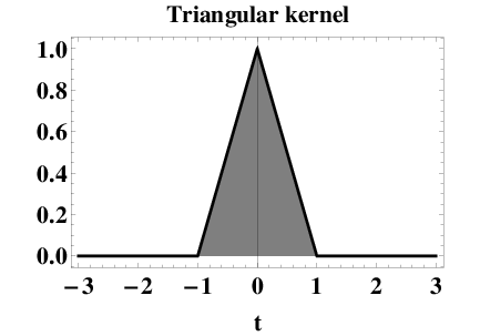


We would like to give important particular cases of IRF’s -integrable components and . Three kernels shown in Figure 1 are chosen under the following motivation:
- •
the triangular kernel is well-known in signal processing as the Bartlett window;
- •
the Laplace kernel is often used for approximation of characteristic functions in harmonic analysis;
- •
the sinc-kernel is an -integrable sign-alternating function which appears in (medical) image processing.
For simplicity, we replace convergence of entropy integrals by sufficient conditions that depend on boundedness of weighted integrals constructed with respect to spectral measures only.
Note that the fact that the outputs and are a. s. continuous means that and are well-defined as elements of ; see (3) and (4), respectively. Remark 3.4 is used in checking the functional CLT. In what follows, stands for the indicator function of a set .
5.1 Examples of the controlled component
By the Fernique theorem (Fernique 1975), a necessary condition for the stationary Gaussian process to be a. s. continuous is that the Dudley integral of be finite: This integral may be bounded from above in terms of the spectral density or the correlation function. In our framework, we will use the already mentioned Hunt condition (e.g., (Cramér and Leadbetter 1967, 196)) stating that if for some the following integral is finite:
| (27) |
then the process is a. s. continuous on .
We give an account of functions satisfying all above assumptions and appearing in a wide range of engineering problems. Next examples represent the scaled classic window functions with bounded (Example 5.1) and unbounded (Example 5.2) supports. All simulations of which are Wiener shot noise processes were made in Wolfram Mathematica 10.4. For more details on similar kernels and their modelling, see (Roberts at el. 2013) and (Prabhu 2014, Chapter 3).
Example 5.1 (Triangular kernel, or the Bartlett window).
For any , put
Framework conditions.
The structure of .
The output is generated by linear filtration of a standard Wiener process:
It is Gaussian stationary zero-mean process; its spectral density is The -like structure of implies that the family converges to a Gaussian white noise as . This property can be traced down in Figure 2 where trajectories of are simulated with increasing values of .


Continuity of .
For any and some , we have
The latter implies condition (27); that is, the controlled process is a. s. continuous on .
Engineering interpretation.
The kernel is defined as a scaled Bartlett window function. This function often appears in problems of linear interpolation and is widely used in signal processing.
Example 5.2 (Exponential kernel, or the Laplace window).
For any , let
Framework conditions.
The structure of .
The output is generated by linear filtration of a standard Wiener process:
In some sense, the last formula is a generalised solution to a Langevin equation describing particle’s velocity in a fluid with unlimited time. It is the well-known Ornstein-Uhlenbeck process on . That is, we deal with a Gaussian stationary zero-mean process with spectral density As we already know, the family converges to a Gaussian white noise as . This fact can be observed in Figure 3 where trajectories of are simulated with increasing values of .


Continuity of . For any and some , we have
The latter implies (27); that is, the controlled output is a. s. continuous on .
Probability interpretation.
The kernel is defined as a normalised (by ) probability density function of the Laplace distribution located at zero and whose scale parameter is . The component may also be interpreted as a normalised (by ) characteristic function of the standard Cauchy distribution with scale parameter . Let us only say that the type of scaling is non-random and is related to harmonic analysis and convolutions involving distribution densities. In some sense, our study uses the inverse Fourier transform for convolutions without assuming absolute integrability of kernels.
5.2 Examples of the unknown component
Recall that, in our framework, the component appears in the functional CLT, in the structure of entropy characteristics and in the construction of confidence intervals. To be more precise:
- •
which is sufficient for CLT of the centred estimator;
- •
Further two examples of IRF kernels are useful in signal and image processing. These examples cover the cases of even and odd ; both functions are defined by continuity at zero.
Example 5.3 (Sinc-kernel, or the Shannon scale function).
Consider the so-called normalised sinc-function
It is clear that ; the Fourier–Plancherel transform of this function is well-known to be
It is clear that and . For any , we have
Therefore satisfies all our assumptions and gives an example of an ideal low-pass filter.
Haar functions and sinc-functions are Fourier duals of each other; it is easy to make calculations in our case. Since is even, is real-valued: . Thus, the correlation function of is as follows:
and the correlation function of has the form
These correlation functions of zero-mean Gaussian processes and are based on the only assumption that is -integrable. The function appears to be the sum of two sinc-waves, one of which is responsible for stationarity (main diagonal) and the second wave “controls” non-stationarity (anti-diagonal). Recall also that in this case
The function in Example 5.3 is the scaling function for the Shannon MRA (signal analysis by ideal bandpass filters). The expression of a real-valued Shannon wavelet can be obtained by taking This wavelet belongs to the -class, but it decreases slowly at infinity and has no bounded support. For a detailed information on Shannon wavelets and their applications, we refer the reader to the book (Najmi 2012, Chapters 4–5).
Our last example shows an odd -integrable function which is a Hilbert transform of the sinc-kernel already mentioned in Example 5.3. In some sense, we save the duality between Haar- and sinc-systems, and show how the fact that is odd affects the characteristics of and .
Example 5.4 (Hilbert transform of the Sinc-kernel).
Take
Of course, one has ; the Fourier–Plancherel transform of is as follows:
It is clear that and For any we have
This means that satisfies all required assumptions. It is a Hilbert transform of an ideal low-pass filter. The fact that is odd implies that is imaginary-valued and . Then the correlation function of is as follows:
and the correlation function of is:
Again the correlation functions of and of are constructed under the only restriction that is -integrable. The correlation function of the non-stationary process splits into two sinc-waves; its shape is quite interesting since .
It follows from Examples 5.3 and 5.4 that the correlation function of the separable Gaussian stationary zero-mean process has the form: Then , , and we can estimate the supremum of using general results in (Cramér and Leadbetter 1967, Chapters 9–10), (Lifshits 1995, Chapters 12–14) or (Adler 2000, Chapter V).
6 Concluding remarks
We gave the principle of estimation the kernels of Wiener shot-noise processes. For this purpose, the LTI SIDO-models were investigated with the Wiener signal as the input. Assuming that one IRF’s component has been controlled, we used the normalized cross-correlogram between outputs as an estimator for the unknown second one. According to the space we chosen, the origin -integrability condition on IRF’s components was reinforced by weighed integrals which were dependent on FRFs of both kernels.
Acknowlegements.
This research was partially supported by the MINECO/FEDER under Grant MTM2015-69493-R. The first author would like to thank the Research Group on Advanced Statistical Modelling (coordinators Prof P. Puig-Casado and J. del Castillo-Franquet) for hospitality during her research stay at the Universitat Autònoma de Barcelona.
References
- 1 Adler, R. J. 2000. An Introduction to Continuity, Extrema, and Related Topics for General Gaussian Processes. Institute of Mathematical Statistics, Harward, CA.
- 2 Anh, V. V., N. N. Leonenko, and L. M. Sakhno. 2007. Statistical inference using higher-order information. Journal of Multivariate Analysis 98 (4): 706–742. doi: 10.1016/j.jmva.2006.09.009.
- 3 Avram, F., N. N. Leonenko, and L. M. Sakhno. 2010. On a Szegö-type limit theorem, the Hölder-Young-Brascamp-Lieb inequality, and the asymptotic theory of integrals and quadratic forms of stationary fields. ESAIM: Probability and Statistics, EDP Sciences, 14: 210–255. doi: 10.1051/ps:2008031.
- 4 Avram, F., N. N. Leonenko, and L. M. Sakhno. 2015. Limit Theorems for additive functionals of stationary fields, under integrability assumptions on the higher order spectral densities. Stochastic Processes and their Applications 125 (4): 1629–1652. doi: 10.1016/j.spa.2014.11.010.
- 5 Blazhievska, I. P. 2011. Correlogram estimation of response functions of linear systems in scheme of some independent samples. Theory of Stochastic Processes 17 (33), no. 1: 16–27. Retrived from http://mi.mathnet.ru/rus/thsp/v17/i1/p16.
- 6 Blazhievska, I., and V. Zaiats. 2018. Estimation of impulse response functions in two-output systems. Communications in Statistics – Theory and Methods: 1-24. doi: 10.1080/03610926.2018.1536210.
- 7 Buldygin, V. V. 1983. On a comparison inequality for the distribution of the maximum of a Gaussian process. Theory of Probability and Mathematical Statistics 28: 9–14. (Russian)
- 8 Bulgygin, V.V., and I.P. Blazhievska. 2009. On asymptotic behaviour of cross-correlogram estimators in linear Volterra Systems. Theory of Stochastic Processes 15 (31), no. 2: 84-98. Retrived from http://mi.mathnet.ru/rus/thsp/v15/i2/p84.
- 9 Buldygin, V. V., and A. B. Kharazishvili. 2000. Geometric Aspects of Probability Theory and Mathematical Statistics. Dordrecht: Springer-Science & Business Media.
- 10 Buldygin, V. V., and Yu. V. Kozachenko. 2000. Metric Characterization of Random Variables and Random Processes (Vol. 188). Providence, Rhode Island: American Mathematical Society.
- 11 Buldygin, V., F. Utzet, and V. Zaiats. 2004. Asymptotic normality of cross-correlogram estimates of the response function. Statistical Inference for Stochastic Processes 7 (1): 1–34. doi: 10.1023/B:SISP.0000016454.89610.35.
- 12 Buldygin, V. V., and V. V. Zaiats. 1991. Comparison theorems and asymptotic behaviour of correlation estimates in spaces of continuous functions. I, II. Ukrainian Mathematical Journal, 444–451; 535–539. doi: 10.1007/BF01058536.
- 13 Buldygin, V. V., and V. V. Zaiats. 1995. On asymptotic normality of estimates for correlation functions of stationary Gaussian processes in the space of continuous functions. Ukrainian Mathematical Journal 47 (11): 1696–1710. doi: 10.1007/BF01057918.
- 14 Camps-Valls, G., J. L. Rojo-Álvarez, and M. Martínez-Ramón. 2007. Kernel Methods in Bioengineering, Signal and Image Processing. Hershey, USA: IGI Global.
- 15 Chen, T., H. Ohlsson, and L. Ljung, 2012. On the estimation of transfer functions, regularizations and Gaussian processes — Revisited. Automatica 48 (8): 1525–1535. doi: 10.1016/j.automatica.2012.05.026.
- 16 Cramér, H., and M. R. Leadbetter. 1967. Stationary and Related Stochastic Processes. New York: John Wiley.
- 17 Demir, A., and A. Sangiovanni-Vincentelli. 1998. Analysis and Simulation of Noise in Nonlinear Electronic Circuits and Systems. New York: Springer Science & Business Media, LLC.
- 18 Dudley, R. M. 1973. Sample functions of the Gaussian processes. The Annals of Probability 1 (1): 66–103.
- 19 Edwards, R. E. 1965. Functional Analysis: Theory and Applications. New York: Holt, Rinehart and Winston.
- 20 Engberg, J., and T. Larsen. 1995. Linear and Nonlinear Circuits. New York: John Wiley & Sons.
- 21 Fernique, X. 1975. Régularité des trajectoires des fonctions aléatoires Gaussiennes. In Ecole d’Eté de Probabilités de Saint-Flour, 1 V-1974, Lecture Notes in Math., 480: 1–96. Springer, Berlin.
- 22 Gao, W., J. Chen, C. Richard, and J. Huang. 2014. Online dictionary learning for kernel LMS. IEEE Transactions on Signal Processing 62 (11): 2765–2777. doi: 10.1109/TSP.2014.2318132.
- 23 Hatemi-J, A. 2012. Asymmetric causality tests with an application. Empirical Economics 43 (1): 447–456. doi: 10.1007/s00181-011-0484-x.
- 24 Hatemi-J, A. 2014. Asymmetric generalized impulse responses with an application in finance. Economic Modelling 36: 18–22. doi: 10.1016/j.econmod.2013.09.014.
- 25 Kolmogorov, A. N. and S. V. Fomin. 1968. Elements of the Theory of Functions and Functional Analysis. Moscow: Nauka. (Russian)
- 26 Kozachenko, Yu. V., and I. V. Rozora. 2015. On cross-correlogram estimators of impulse response functions. Theory Probability and Mathematical Statistics 93: 75–86. doi: 10.1090/tpms/995. (Ukrainian)
- 27 Kozachenko, Yu. V., T. V. Hudyvok, V. B. Troshki, and N. V. Troshki. 2017. Estimation of Covarience Functions of Gaussian Stochastic Fields and Their Simulation. Uzhhorod: AUDOR-Shark.
- 28 Ledoux, M, and M. Talagrand. 2013. Probability in Banach Spaces: Isoperimetry and Processes. Springer Science & Business Media.
- 29 Li, F. 2005. Asymptotic properties of an estimator of an impulse response function in linear two-dimensional systems. Bulletin BGU (Physics. Mathematics. Informatics) 1: 93–99 (Russian).
- 30 Lifshits, M. A. 1995. Gaussian Random Functions (Vol. 322). Springer Netherlands: Springer Science & Business Media Dordrecht.
- 31 Lindgren, G. 2006. Lectures on Stationary Stochastic Processes. Accessed Abril 19, 2018. http://www.maths.lth.se/matstat/staff/georg/Publications/lecture2006.pdf.
- 32 Marcus, M. B. and L. A. Shepp. 1972. Sample behavior of Gaussian processes. In: Proc. Sixth Berkeley Symp. on Mathem. Statist. and Probab., vol. 2: Probability Theory, 423–441, University of California Press, Berkeley, CA. Retrived from https://projecteuclid.org/euclid.bsmsp/1200514231.
- 33 Najmi A.-H. 2012. Wavelets: A Concise Guide. Baltimore: The Johns Hopkins University Press.
- 34 Nourdin, I., G. Peccati, and F. G. Viens. 2014. Comparison inequalities on Wiener space. Stochastic Processes and their Applications 124: 1566–1581. doi: 10.1016/j.spa.2013.12.001.
- 35 Ogunfunmi, T. 2007. Adaptive Nonlinear System Identification: The Volterra and Wiener Model Approaches. New York: Springer Science & Business Media.
- 36 Prabhu, K. M. M. 2014. Window Functions and Their Application in Signal Processing. CRC Press: Taylor & Francis Group.
- 37 Ren, W.-X., T. Zhao, and I.E. Harik. 2004. Experimental and analytical modal analysis of a steel arch bridge, Journal of Structural Engineering, 130 (7): 1022–1031. doi: 10.1061/(ASCE)0733-9445(2004)130:7(1022).
- 38 Roberts S., M. Osborne, M. Ebden, S. Reece, N. Gibson, and S. Aigrain. 2013. Gaussian processes for time-series modelling. Philosophical Thansactions of the Royal Society A 371: 20110550. doi: 10.1098/rsta.2011.0550.
- 39 Rost, E., R. Geske, and M. Baake. 2006. Signal analysis of impulse response functions in MR and CT measurements of cerebral blood flow. Journal of Theoretical Biology 240: 451–458. doi: 10.1016/j.jtbi.2005.10.005.
- 40 Rozora, I. V. 2018. Statistical hypothesis testing for the shape of impulse response function. Communications in Statistics–Theory and Methods 47 (6): 1459–1474. doi: 10.1080/03610926.2017.1321125.
- 41 Sjöberg, J., Q. Zhang, L. Ljung, A. Benveniste, B. Delyon, P.-Y. Glorennec, H. Hjalmarsson, and A. Juditsky. 1995. Nonlinear black-box modeling in system identification: a unified overview. Automatica 31 (12): 1691–1724. doi: 10.1016/0005-1098(95)00120-8.
- 42 Söderström, T., and P. Stoica. 1988. System Identification. London: Prentice-Hall.
- 43 Spiridonakos, M. D., and E. N. Chatzi. 2014. Stochastic structural identification from vibrational and environmental data. In: Beer M., I. Kougioumtzoglou, E. Patelli, and IK. Au. (eds.) Encyclopedia of Earthquake Engineering. Springer, Berlin, Heidelberg. doi: 10.1007/978-3-642-36197-5.