Linkage Mechanisms Governed by Integrable Deformations of Discrete Space Curves
Shizuo Kaji1, Kenji Kajiwara2
Institute of Mathematics for Industry, Kyushu University
744 Motooka, Fukuoka 819-0395, Japan
e-mail: 1skaji@imi.kyushu-u.ac.jp, 2kaji@imi.kyushu-u.ac.jp
Hyeongki Park
Graduate School of Mathematics, Kyushu University
744 Motooka, Fukuoka 819-0395, Japan
e-mail: h-park@math.kyushu-u.ac.jp
Abstract
A linkage mechanism consists of rigid bodies assembled by joints which can be used to translate and transfer motion from one form in one place to another. In this paper, we are particularly interested in a family of spatial linkage mechanisms which consist of -copies of a rigid body joined together by hinges to form a ring. Each hinge joint has its own axis of revolution and rigid bodies joined to it can be freely rotated around the axis. The family includes the famous threefold symmetric Bricard 6R linkage, also known as the Kaleidocycle, which exhibits a characteristic “turning-over” motion. We can model such a linkage as a discrete closed curve in of constant torsion up to sign. Then, its motion is described as the deformation of the curve preserving torsion and arc length. We describe certain motions of this object that are governed by the semi-discrete mKdV and sine-Gordon equations, where infinitesimally the motion of each vertex is confined in the osculating plane.
1 Introduction
A linkage is a mechanical system consisting of rigid bodies (called links) joined together by joints. They are used to transform one motion to another as in the famous Watt parallel motion and a lot of examples are found in engineering as well as in natural creatures (see, for example, [7]).
Mathematical study of linkage dates back to Euler, Chebyshev, Sylvester, Kempe, and Cayley and since then the topology and the geometry of the configuration space have attracted many researchers (see [12, 24, 31] for a survey). Most of the research focuses on pin joint linkages, which consist of only one type of joint called pin joints. A pin joint constrains the positions of ends of adjacent links to stay together. To a pin joint linkage we can associate a graph whose vertices are joints and edges are links, where edges are assigned its length. The state of a pin joint linkage is effectively specified by the coordinates of the joint positions, where the distance of two joints connected by a link is constrained to its length. Thus, its configuration space can be modelled by the space of isometric imbeddings of the corresponding graph to some Euclidean space. Note that in practice, joints and links have sizes and they collide to have limited mobility, but here we consider ideal linkages with which joints and links can pass through each other.
While the configuration spaces of (especially planar) pin joint linkages are well studied, there are other types of linkages which are not so popular. In this chapter, we are mainly interested in linkages consisting of hinges (revolute joints). To set up a framework to study linkages with various types of joints, we first introduce a mathematical model of general linkages as graphs decorated with groups (§2.1), extending previous approaches (see [34] and references therein). This formulation can be viewed as a special type of constraint network (e.g., [14]). Then in §2.2, we focus on linkages consisting of hinges. Unlike a pin joint which constrains only the relative positions of connected links, a hinge has an axis so that it also constrains the relative orientation of connected links.
We are particularly interested in a simple case when links in are joined by hinges to form a circle (§3). Such a linkage can be roughly thought of as a discrete closed space curve, where hinge axes are identified with the lines spanned by the binormal vectors. Properties of such linkages can thus be translated and stated in the language of discrete curves. An example of such linkage is the threefold symmetric Bricard 6R linkage consisting of six hinges (Fig. 1), which exhibits a turning-over motion and has the configuration space homeomorphic to a circle. As a generalisation to the threefold symmetric Bricard 6R linkage, we consider a family of linkages consisting of copies of an identical links connected by hinges, which we call Kaleidocycles, and they are characterised as discrete curves of constant speed and constant torsion.

The theory of discrete space curves has been studied by many authors. The simplest way to discretise a space curve is by a polygon, that is, an ordered sequence of points . Deformation of a curve is a time-parametrised sequence of curves , where runs through (an interval of) the real numbers. Deformations of a given smooth/discrete space curve can be described by introducing an appropriate frame such as the Frenet frame, which satisfies the system of linear partial differential/differential-difference equations. The compatibility condition gives rise to nonlinear partial differential/differential-difference equation(s), which are often integrable. It is sometimes possible to construct deformations for the space curves using integrable systems which preserve some geometric properties of the space curve such as length, curvature, and torsion. For example, a deformation is said to be isoperimetric if the deformation preserves the arc length. In this case, the modified Korteweg-de Vries (mKdV) or the nonlinear Schrödinger (NLS) equation and their hierarchies naturally arise as the compatibility condition [6, 10, 15, 18, 27, 28, 37, 41]. Various continuous deformations for the discrete space curves have been studied in [11, 16, 18, 36, 38], where the deformations are described by the differential-difference analogue of the mKdV and the NLS equations.
The motion of Kaleidocycles corresponds to isoperimetric and torsion-preserving deformation of discrete closed space curves of constant torsion. In §4, we define a flow on the configuration space of a Kaleidocycle by the differential-difference analogue of the mKdV and the sine-Gordon equations (semi-discrete mKdV and sine-Gordon equations). This flow generates the characteristic turning-over motion of the Kaleidocycle.
Kaleidocycles exhibit interesting properties and pose some topological and geometrical questions. In §5 we indicate some directions of further study to close this exposition.
We list some more preceding works in different fields which are relevant to our topic in some ways.
Mobility analysis of a linkage mechanism studies how many degrees of freedom a particular state of the linkage has, which corresponds to determination of the local dimension at a point in the configuration space (see, for example, [35]). On the other hand, rigidity of linkages consisting of hinges are studied in the context of the body-hinge framework (see, for example, [20, 25]). The main focus of the study is to give a characterisation for a generic linkage to have no mobility. That is, the question is to see if the configuration space is homeomorphic to a point or isolated points.
Sato and Tanaka [42] study the motion of a certain linkage mechanism with a constrained degree of freedom and observed that soliton solutions appear.
2 A mathematical model of linkage
The purpose of this section is to set up a general mathematical model of linkages. This section is almost independent of later sections, and can be skipped if the reader is concerned only with our main results on the motion of Kaleidocycles.
2.1 A group theoretic model of linkage
We define an abstract linkage as a decorated graph, and its realisation as a certain imbedding of the graph in a Euclidean space. Our definition generalises the usual graphical model of a pin joint linkage to allow different types of joints.
Denote by the group of orientation preserving linear isometries of the -dimensional Euclidean space . An element of is identified with a sequence of -dimensional column vectors which are mutually orthogonal and have unit length with respect to the standard inner product of . Denote by the group of -dimensional orientation preserving Euclidean transformations. That is, it consists of the affine transformations which preserves the orientation and the standard metric. We represent the elements of by homogeneous matrices acting on
by multiplication from the left. For example, an element of is represented by a matrix
The vector is called the translation part. The upper-left -block of is called the linear part and denoted by . Thus, the action on is also written by .
Definition 1.
An -dimensional abstract linkage consists of the following data:
- •
a connected oriented finite graph
- •
a subgroup assigned to each , which defines the joint symmetry
- •
an element assigned to each , which defines the link constraint.
In practical applications, we are interested in the case when or . When linkages are said to be planar, and when linkages are said to be spatial.
We say a linkage is homogeneous if for any pair , the following conditions are satisfied:
- •
there exists a graph automorphism which maps to (i.e., acts transitively on ),
- •
,
- •
and for any .
A state or realisation of an abstract linkage is an assignment of a coset to each vertex
such that for each edge , the following condition is satisfied:
| (2.1) |
where cosets are identified with subsets of .
Let us give an intuitive description of (2.1). Imagine a reference joint sitting at the origin in a reference orientation. The subset consists of all the rigid transformations which maps the reference joint to the joint at with a specified position and an orientation up to the joint symmetry . The two subsets and intersects if and only if the joint at can be aligned to that at by the transformation .
Example 1.
The usual pin joints connected by a bar-shaped link of length are represented by and being any translation by . Note that . It is easy to see that (2.1) amounts to saying the difference in the translation part of and should have the norm equal to .
Two revolute joints (hinges) in connected by a link of length making an angle are represented by being the group generated by rotations around the -axis and the -rotation around the -axis, and being the rotation by around -axis followed by the translation along -axis by ; that is
Note that is the space of based lines (i.e., lines with specified origins) in , and the line is identified with the axis of the hinge.
The space of all realisations of a given linkage admits an action of defined by for . The quotient of by is denoted by and called the configuration space of . Each connected component of corresponds to the mobility of the linkage in a certain state. When a connected component is a manifold, its dimension is what mechanists call the (internal) degrees of freedom (DOF, for short). Given a pair of points on , the problem of finding an explicit path connecting the points is called motion planning and has been one of the main topics in mechanics [30]. In a similar manner, many questions about a linkage can be phrased in terms of the topology and the geometry of its configuration space.
Example 2.
Consider the following spatial linkages consisting of pin joints depicted in Figure 2. In the latter, we assume the two joints and are fixed to the wall. Up to the action of the global rigid transformation , these two linkages are equivalent and share the same configuration space ; in the left linkage, the global action is killed by fixing the positions of three joints except for .


The topology of changes with respect to the parameter which is the length of the bars. Namely, we have
This seemingly trivial example is indeed related to a deeper and subtle question on the topology of the configuration space; the space is identified with the real solutions to a system of algebraic equations.
2.2 Hinged linkage in three space
Now, we focus on a class of spatial linkages consisting of hinges, known also as three dimensional body-hinge frameworks [20]. In this case, the definition in the previous section can be reduced to a simpler form.
Notice that in a pair of hinges connected by a link can be modelled by a tetrahedron. A hinge is an isometrically embedded real line in . Given a pair of hinges, unit-length segments on the hinges containing the base points in the centre span a tetrahedron, or a quadrilateral when the two hinges are parallel (see Fig. 3 Left). It is sometimes convenient to decompose the link constraint into three parts; a translation along the hinge direction at , a screw motion along an axis perpendicular to both hinges, and a translation along the hinge direction at . This corresponds to a common presentation among mechanists called the Denavit–Hartenberg parameters [9]. We can find the decomposition geometrically as follows: Find a line segment which is perpendicular to the both hinges connected by the link , which we call the core segment. It is unique unless the hinges are parallel. The intersection points of the core segment and the hinges are called the marked points. Form a tetrahedron from the line segments on hinges containing the marked points in the centre. By construction, this tetrahedron has a special shape that the line connecting the centre of two hinge edges (the core segment) is perpendicular to the hinge edges. Such a tetrahedron is called a disphenoid. The shape of the disphenoid defines a screw motion along the core segment up to a -rotation. The translations along the hinge directions are to match the marked points to the base points (see Fig. 3). To sum up, a spatial hinged linkage can be considered as a collection of lines connected by disphenoids at marked points.


Thus, we arrive in the following definition.
Definition 2.
A hinged network consists of
- •
a connected oriented finite graph ,
- •
two edge labels called the torsion angle and called the segment length,
- •
and a vertex label called the marking, where is the set of edges adjacent to .
A state of a hinged network is an assignment to each vertex of an isometric embedding such that for any
- 1.
, where
- 2.
and
- 3.
, where the angle is measured in the left-hand screw manner with respect to .
Intuitively, is the line spanned by the hinges, and the first two conditions demand that the marked points are connected by the core segments , whereas the last condition dictates the torsion angle of adjacent hinges and .
A hinged network is said to be serial when the graph is a line graph; i.e., a connected graph of the shape . It is said to be closed when the graph is a circle graph; i.e., a connected finite graph with every vertex having outgoing degree one and incoming degree one. A hinged network is homogeneous if
- •
acts on transitively,
- •
, and do not depend on and . That is, it is made of congruent tetrahedral links.
Example 3.
A planar pin joint linkage is a special type of hinged network with for all and for all . That is, all hinges are parallel and marked points are all at the origin. On the other hand, any hinged network can be thought of as a spatial pin joint linkage by replacing every tetrahedral link with four bar links connected by four pin joints forming the tetrahedron. Therefore, hinged networks form an intermediate class of linkages which sits between planar pin joint linkages and spatial pin joint linkages.

Example 4.
The hinged network depicted in Fig. 5 is over the wedge sum of two circle graphs. It exhibits a jump roping motion. A similar but more complex network is found in [7, §6].

Example 5.
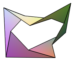
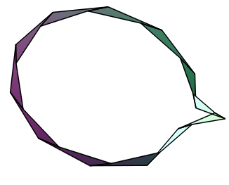
Closed hinged networks with (that is, adjacent hinge lines intersect) for all provide a linkage model for discrete developable strips studied recently by K. Naokawa and C. Müller (see Fig. 6). They are made of (planar) quadrilaterals joined together by the pair of non-adjacent edges as hinges.
3 Hinged network and discrete space curve
In this section, we describe a connection between spatial closed hinged networks and discrete closed space curves. This connection is the key idea of this chapter which provides a way to study certain linkages using tools in discrete differential geometry.
First, we briefly review the basic formulation of discrete space curves (see, for example, [18]). A discrete space curve is a map
For simplicity, in this chapter we always assume that for any and that three points , and are not colinear. The tangent vector is defined by
| (3.1) |
We say has a constant speed of if for all . A discrete space curve with a constant speed is sometimes referred to as an arc length parametrised curve [17]. The normal vector and the binormal vector are defined by
| (3.2) | ||||
| (3.3) |
respectively. Then, is called the Frenet frame of . For our purpose, it is more convenient to use a modified version of the ordinary Frenet frame, which we define as follows. Set and define recursively so that and . Then, , where (see Fig. 7).

For , we define by
| (3.4) |
There exist and such that
| (3.5) |
We call the signed curvature angle and the torsion angle. Fig. 8 illustrates how to obtain from by (3.5). Note that we have
| (3.6) |

The reason why we introduce the modified frame is that the ordinary Frenet frame behaves discontinuously under deformation when the ordinary curvature angle vanishes at a point. During the turning-over motion of a Kaleidocycle, it goes through such a state at some points, and the above modified frame behaves consistently even under the situation.
Fix a natural number . A discrete space curve is said to be closed of length if for any . Unlike the ordinary Frenet frame, closedness does not imply but they may differ by rotation by around . We say is oriented (resp. anti-oriented) if (resp. ) for all .
We can consider a discrete version of the Darboux form [8, 46], which gives a correspondence between spherical curves and space curves. Given with for all and , we can associate a discrete space curve satisfying
| (3.7) |
which we denote by . The curve is closed of length if
| (3.8) |
for all .
Notice that a serial (resp. closed) hinged network with for all (see Def. 2) can be modelled by an open (resp. a closed) discrete space curve; its base points form the curve and hinge directions are identified with (see Fig. 9). This is the crucial observation of this chapter.

Now we introduce our main object, Kaleidocycles, which are homogeneous closed hinged networks. We model them as constant speed discrete space curves of constant torsion. They are a generalisation to a popular paper toy called the Kaleidocycle (see, e.g., [4, 43]). A serial hinged network similar to our Kaleidocycle is proposed in [33].
Definition 3.
Fix and . An -Kaleidocycle with a speed and a torsion angle is a closed discrete space curve of length which has a constant speed and a constant torsion angle . It is said to be oriented (resp. anti-oriented) when associated is oriented (resp. anti-oriented).
When is either or , the corresponding Kaleidocycles are planar, and we call them degenerate.


For fixed and , an oriented (resp. anti-oriented) non-degenerate Kaleidocycle with a torsion angle is determined by the Darboux form by a map satisfying p
- •
(resp. ),
- •
,
- •
.
We use and interchangeably to represent a Kaleidocycle.
Consider the real algebraic variety defined by the following system of quadratic equations ([44, Ex. 5.2, 8.13]):
| (3.9) |
where is considered as an indeterminate. The orthogonal group acts on ’s in the standard way, and hence, on . Denote by the quotient of by the action of . The variety serves as the configuration space of all -Kaleidocycles with varying . It decomposes into two disjoint sub-spaces consisting of all oriented Kaleidocycles () and consisting of anti-oriented ones ().
As (resp. ) is a closed variety, its image under the projection onto the -axis is a union of closed intervals. Notice that the image does not coincide with the whole interval ; means are all equal so we cannot have . The fibre consists of -Kaleidocycles with a fixed . With a generic value of , a simple dimension counting in (3.9) shows that . Hence, the degree of freedom (DOF) of the Kaleidocycle with a torsion angle is generally . For , a generic Kaleidocycle is reconfigurable meaning that it can continuously change its shape. We will investigate a particular series of reconfiguration in the next section.
4 Deformation of discrete curves
4.1 Continuous isoperimetric deformations on discrete curves
Kaleidocycles exhibit a characteristic turning-over motion (see Fig. 11 and see [22] for some animations). In general, an -Kaleidocycle has degrees of freedom so that it wobbles in addition to turning-over. With special values of torsion angle, however, the DOF of the Kaleidocycle seems to degenerate to exactly one, leaving only the turning-over motion as we will discuss in §5. In this case, the motion of the core segment looks to be orthogonal to the hinge directions. In the following, we would like to model the motion explicitly. It turns out that we can construct the motion of Kaleidocycles using semi-discrete mKdV and sine-Gordon equations.


In this section, we consider certain continuous deformations of discrete space curves which correspond to motion of homogeneous serial and closed hinged networks. Our approach is to construct a flow on the configuration space by differential-difference equations. We use the same notations as in Section 3. Observe that a hinged network moves in such a way that its tetrahedral links are not distorted. In the language of discrete space curves, the motion corresponds to a deformation which preserves the speed and the torsion angle for all .
Let be an (open) discrete space curve which has a constant speed and a constant torsion angle . Given a family of functions with the deformation parameter and a constant , we consider a family of discrete space curves defined by
| (4.1) |
That is, the motion of each point is confined in the osculating plane and its speed depends only on the length of the segment . We say a deformation is isoperimetric if the segment length does not depend on for all , We would like to find conditions on under which the above deformation is isoperimetric. From (3.1), (3.5) and (4.1), we have
Therefore, for each , vanishes if and only if
| (4.2) |
which yields
| (4.3) |
or
| (4.4) |
We consider a deformation when (4.3) (resp. (4.4)) simultaneously holds for all . Note that in this case for all is determined once is given.
Those deformations are characterised by the following propositions:
Proposition 1.
Let be a discrete space curve with a constant speed and a constant torsion angle . Let be its deformation according to (4.1) with satisfying the condition (4.3). Then we have:
- 1.
The speed and the torsion angle do not depend on nor . That is, and for all and .
- 2.
The signed curvature angle and satisfy
(4.5) where .
- 3.
The deformation of the frame is given by
(4.6)
Proposition 2.
Let be a discrete space curve with a constant speed and a constant torsion angle . Let be its deformation according to (4.1) with satisfying the condition (4.4). Then we have:
- 1.
The speed and the torsion angle do not depend on nor . That is, and for all and .
- 2.
The signed curvature angle and satisfy
(4.7) where .
- 3.
The deformation of the frame is given by
(4.8)
Proof.
We only prove Proposition 1 since Proposition 2 can be proved in the same manner. We first show the second and the third statements. We denote , and for simplicity. Since is a constant by the preceding argument, the deformation of can be computed from (4.1) and (4.4) as
| (4.9) |
Differentiating with respect to , we have
| (4.10) |
Noting
| (4.11) |
and
| (4.12) |
| (4.13) |
which is equivalent to (4.7). This proves the second statement. Next, we see from the definition of
| (4.14) |
Noting
| (4.15) |
| (4.16) |
and
| (4.17) |
| (4.18) |
We immediately obtain from (4.9) and (4.14) as
| (4.19) |
Then we have (4.8) from (4.9), (4.14) and (4.19), which proves the third statement. Finally, differentiating with respect to , it follows from (4.18) and (4.2) that
which implies . This completes the proof of the first statement. ∎
Remark 2.
The condition (4.3) suggests the potential function in Proposition 1 such that we have
| (4.20) |
Then, (4.5) is rewritten as
| (4.21) |
To the best of the authors’ knowledge, this is a novel form of the semi-discrete potential mKdV equation. In fact, the continuum limit , , , yields the potential mKdV equation
| (4.22) |
Similarly, introducing the potential function in Proposition 2 such that
| (4.23) |
suggested by (4.4), we can rewrite (4.7) as
| (4.24) |
which is nothing but the semi-discrete sine-Gordon equation [3, 39, 40].
Remark 3.
In the above argument, we assume that the speed of the deformation in (4.1) is a constant and does not depend on . Then, by demanding that the deformation preserve arc length ((4.3) or (4.4)), it followed that the torsion angle is also preserved. Conversely, it seems to be the case that for the deformation to preserve both the arc length and the torsion angle, the speed is required not to depend on .
Remark 4 (Continuum limit).
The isoperimetric torsion-preserving discrete deformations for the discrete space curves of constant torsion have been considered in [18], where the deformations are governed by the discrete sine-Gordon and the discerte mKdV equations. It is possible to obtain the continuous deformations discussed in this section by suitable continuum limits from those discrete deformations. More precisely, let () be a family of discrete curves obtained by applying the discrete deformations times to , where is the discrete curve with a constant speed and a constant torsion angle . Then the above discrete deformation is given by
| (4.25) |
Then if we choose and so that the sign of does not depend on , the isoperimetric condition and the compatibility condition of the Frenet frame yield the discrete mKdV equation
| (4.26) |
when , and the discrete sine-Gordon equation
| (4.27) |
when with
| (4.28) |
For the discrete mKdV equation (4.26), in the limit of
| (4.29) |
(4.26) is reduced to the semi-discrete mKdV equation (4.5). Similarly, the discrete sine-Gordon equation (4.27) is reduced to the semi-discrete sine-Gordon equation (4.7) in the limit
| (4.30) |
Obviously, the discrete deformation equation of the discrete curve (4.25) is reduced to the continuous deformation equation (4.1). Moreover, it is easily verified that the discrete deformation equations of the Frenet frame in [18] are reduced to (4.6) and (4.8).
4.2 Turning-over motion of Kaleidocycles
An -Kaleidocycle corresponds to a closed discrete curve of length having a constant speed and a constant torsion angle whose is oriented. Since is closed, for (4.1) to define a deformation of , we need a periodicity condition (when oriented) or (when anti-oriented) for any .
When is odd and the Kaleidocycle is oriented, the equation (4.3) together with forms a linear system for which is regular. Therefore, we can find uniquely as the solution to the system. Then, the equation (4.1) generates a deformation of which preserves the segment length and the torsion angle, while remains closed. That is, the turning-over motion of the Kaleidocycle is governed by the semi-discrete mKdV equation (4.5) (see Fig. 12). Note that by (4.5), the total curvature angle is also preserved.


When the Kaleidocycle is anti-oriented, the equation (4.4) together with forms a linear system for which is regular for any . Similarly to the above, in this case the turning-over motion of the Kaleidocycle is governed by the semi-discrete sine-Gordon equation (4.7).
Note that if an -Kaleidocycle with an odd is anti-oriented , we can define an oriented Kaleidocycle by taking its “mirrored image” which conforms to the definition 3. Thus, for an odd Kaleidocycle, both the semi-discrete mKdV equation and the semi-discrete sine-Gordon equation generate the turning-over motion.
5 Extreme Kaleidocycles
We defined Kaleidocycles in Def. 3 and saw the torsion angle cannot be chosen arbitrarily. A natural question is for what torsion angle there exists an -Kaleidocycle for each . It seems there are no Kaleidocycles with for . For , we conducted numerical experiments with [22] and found that there exists which satisfy the following. Recall that is the projection of the configuration space onto the -axis, where .
- 1.
When is odd, and .
- 2.
When is even, and .
Moreover, converges monotonously to a constant, where takes the principal value in . Interestingly, at the boundary values , the fibre of seems to be exactly one-dimensional for any . This means, they are exactly the one-dimensional orbits defined in §4.2.
We summarise our numerical findings.
Conjecture 1.
Let . We have the following:
- 1.
The space is a circle. Moreover, the involution defined by induces isomorphisms when is odd and when is even.
- 2.
The orbit of any element of the flow generated by the semi-discrete sine-Gordon equation described in §4.2 coincides with .
- 3.
When is odd, the orbit of any element generated by the semi-discrete mKdV equation described in §4.2 coincides with . Moreover, on we have and we can also define its deformation by the semi-discrete sine-Gordon equation if we define by (4.4) and . The orbit coincides with as well. That is, for an oriented Kaleidocycle with , we can define two motions one by the semi-discrete sine-Gordon equation (4.4), the other by the semi-discrete mKdV equation (4.3), and they coincide up to rigid transformations.
- 4.
Any strip corresponding to is a 3-half twisted Möbius strip (see §5.2). There are no Kaleidocycles with one or two half twisting.
- 5.
When tends to infinity, converges to a constant. There exists a unique limit curve up to congruence for any sequence , and it has a constant torsion up to sign.
We call those Kaleidocycles having the extremal torsion angle extreme Kaleidocycles.
Remark 5.
The extreme Kaleidocycles were discovered by the first named author and his collaborators [21, 23]. In particular, when it is anti-oriented, it is called the Möbius Kaleidocycle because they are a discrete version of the Möbius strip with a -twist. Coincidentally, Möbius is the first one to give the dimension counting formula for generic linkages [32] (although it is often attributed to Maxwell), and our Möbius Kaleidocycles are exceptions to his formula.
We end this chapter with a list of interesting properties, questions and some supplementary materials of Kaleidocycles for future research.
5.1 Kinematic energy
Curves with adapted frames serve as a model of elastic rods and are studied, for example, in Langer and Singer [29] in a continuous setting, and in [2] in a discrete setting. Serial and closed hinged networks are discrete curves with specific frames as we saw in §3. From this viewpoint, we consider some energy functionals defined for discrete curves with frames and investigate how they behave on the configuration space of Kaleidocycles.
Let be a constant speed discrete closed curve of length . The elastic energy and the twisting energy are defined respectively by
By the definition of Kaleidocycle, takes a constant value when a Kaleidocycle undergoes any motion.
Interestingly, a numerical simulation by [22] suggests that on (and also on for an odd and on for an even ) for a fixed , takes an almost constant value. The summands of are locally determined and vary depending on the states, however, the total is almost stable so that only small force should be applied to rotate the Kaleidocycle. It is also noted that the sum is a discrete version of the elastic energy of the Kirchoff rod defined by the strip, and it also takes almost constant values.
Similarly, we introduce the following three more energy functionals, which are observed to take almost constant values on . The dipole energy is defined to be
The Coulomb energy with an exponent is defined to be
The averaged hinge magnitude is defined to be
However, we have no rigorous statements about them. It may be the case that one needs some other discretisation of the continuous counterparts of these energies to show their behaviour theoretically. It is also interesting to characterise or generalise extreme Kaleidocycles in terms of variational calculus on the space of discrete closed curves.
5.2 Topological invariants
As noted in [29], for a curve to be closed, topological constraints come into the story. This quantises some continuous quantity and makes it an isotopy invariant.
Let be a constant speed discrete closed curve of length . First, interpolate and for linearly to obtain a continuous vector field defined on the polygonal curve , which goes around the polygon twice. We define the twisting number of as the linking number between twice the centre curve and the boundary curve , where is small enough.

Intuitively, it is the number of half-twists of the strip defined by and . The Cǎlugǎreanu-White formula relates this topological invariant to the sum of two conformal invariants and provides a direct discretisation without the need of interpolation (cf. [26]):
| (5.1) |
where is the writhe of the polygonal curve which can be computed as a double summation [26, Eq. (13)] and
is the total twist. The twisting number takes values in the integers, enforcing topological constraints to the curve.
Recall by definition that anti-oriented extreme Kaleidocycles are discrete closed space curves of constant speed and constant torsion which have the minimum odd twisting number. Our numerical experiments suggest that the minimum is not one but three.
Let be a discrete closed space curve of constant speed and constant torsion corresponding to a Kaleidocycle. Under any motion of the Kaleidocycle, stays constant by definition. By (5.1) the corresponding deformation of the curve preserves the writhe as well. This can equivalently be phrased in terms of the Gauss map . The Gauss-Bonnet theorem tells us that , where is the area on the sphere enclosed by . By (5.1) we have . Thus, the deformation of the closed discrete space curve considered in §4.2 induces one of the closed discrete spherical curves which preserves the enclosed area .
Kaleidocycles can be folded from a piece of paper. We include a development plan for the extreme Kaleidocycle with so that the readers can personally make and investigate its motion.

Acknowledgments.
The first named author is partially supported by JST, PRESTO Grant Number JPMJPR16E3, Japan. The second named author is partially supported by JSPS KAKENHI Grant Numbers JP16H03941, JP16K13763. The last named author acknowledges the support from the “Leading Program in Mathematics for Key Technologies” of Kyushu University.
References
- [1] Bates L M and Melko O M, On curves of constant torsion I, Journal of Geometry, 104(2), 213–227, 2013.
- [2] Bergou M, Wardetzky M, Robinson S, Audoly B and Grinspun E, Discrete elastic rods, ACM Trans. Graph., 27(3), Article 63, 2008.
- [3] Boiti M, Pempinelli F and Prinari B, Integrable discretization of the sine-Gordon equation, Inverse Problems 18(5), 1309–1324, 2002.
- [4] Byrnes R, Metamorphs: Transforming Mathematical Surprises, Tarquin Pubns, 1999.
- [5] Calini A M, Ivey T A, Bäcklund transformations and knots of constant torsion, J. Knot Theory Ram., 7, 719–746, 1998.
- [6] Calini A M an Ivey T A, Topology and sine-Gordon evolution of constant torsion curves, Phys. Lett. A, 254(3–4), 170–178, 1999.
- [7] You Z and Chen Y, Motion Structures: Deployable Structural Assemblies of Mechanisms, Taylor & Francis, 2011.
- [8] Darboux G, Leçcons sur la Théorie Générale des Surfaces, Gauthier-Villars, 1917.
- [9] Denavit J and Hartenberg R S, A kinematic notation for lower-pair mechanisms based on matrices, Trans ASME J. Appl. Mech. 23, 215–221, 1955.
- [10] Doliwa A and Santini P M, An elementary geometric characterization of the integrable motions of a curve, Phys. Lett. A, 185, 373–384, 1994.
- [11] Doliwa A and Santini P M, Integrable dynamics of a discrete curve and the Ablowitz-Ladik hierarchy, J. Math. Phys. 36, 1259–1273, 1995.
- [12] Farber M, Invitation to Topological Robotics, European Mathematical Society, Zurich, 2008.
- [13] Fowler P W and Guest S D, A symmetry analysis of mechanisms in rotating rings of tetrahedra, Proc. R. Soc. A 461, 1829–1846, 2005.
- [14] Freuder E C, Synthesizing constraint expressions, Commun. ACM 21(11), 958–966, 1978.
- [15] Hasimoto H, A soliton on a vortex filament, J. Fluid. Mech. 51, 477–485, 1972.
- [16] Hisakado M and Wadati M, Moving discrete curve and geometric phase, Phys. Lett. A, 214, 252–258, 1996.
- [17] Hoffmann T, Discrete Differential Geometry of Curves and Surfaces, MI Lecture Notes vol. 18, Kyushu University, 2009.
- [18] Inoguchi J, Kajiwara K, Matsuura N and Ohta Y, Discrete mKdV and discrete sine-Gordon flows on discrete space curves, J. Phys. A: Math. Theor. 47, 2014.
- [19] Ivey T A, Minimal Curves of Constant Torsion, Proc. AMS, 128(7), 2095–2103, 2000.
- [20] Jordán T, Király C and Tanigawa S, Generic global rigidity of body-hinge frameworks, J. Comb. Theory B, 117, 59–76, 2016.
- [21] Kaji S, A closed linkage mechanism having the shape of a discrete Möbius strip, the Japan Society for Precision Engineering Spring Meeting Symposium Extended Abstracts, 62–65, 2018. The original is in Japanese but an English translation is available at arXiv:1909.02885.
- [22] Kaji S, Geometry of the moduli space of a closed linkage: a Maple code, available at https://github.com/shizuo-kaji/Kaleidocycle
- [23] Kaji S, Schönke S, Grunwald M and Fried E, Möbius Kaleidocycle, patent filed, JP2018-033395, 2018.
- [24] Kapovich M and Millson J, Universality theorems for configuration spaces of planar linkages, Topology 41(6), 1051–1107, 2002.
- [25] Katoh N and Tanigawa S, A proof of the molecular conjecture, Discrete Comput Geom., 45, 647–700, 2011.
- [26] Klenin K and Langowski J, Computation of writhe in modeling of supercoiled DNA, Biopolymers, 54, 307–317, 2000.
- [27] Lamb G L Jr., Solitons and the motion of helical curves, Phys. Rev. Lett. 37, 235–237, 1976.
- [28] Langer J and Perline R, Curve motion inducing modified Korteweg-de Vries systems, Phys. Lett. A, 239, 36–40, 1998.
- [29] Langer J and Singer D A, Lagrangian aspects of the Kirchhoff elastic rod, SIAM Review 38(4), 605–618, 1996.
- [30] LaValle S M, Planning algorithms, Cambridge University Press, 2006.
- [31] Magalhães M L S and Pollicott M, Geometry and dynamics of planar linkages, Comm. Math. Phys., 317(3), 615–634, 2013.
- [32] Möbius A F, Lehrbuch der Statik, 2, Leipzig, 1837.
- [33] Moses M S and Ackerman M K and Chirikjian G S, ORIGAMI ROTORS: Imparting continuous rotation to a moving platform using compliant flexure hinges, Proc. IDETC/CIE 2013.
- [34] Müller A, Representation of the kinematic topology of mechanisms for kinematic analysis, Mech. Sci., 6, 1–10, 2015.
- [35] Müller A, Local kinematic analysis of closed-loop linkages – mobility, singularities, and shakiness, J. Mechanisms Robotics 8(4), 041013, 2016.
- [36] Nakayama K, Elementary vortex filament model of the discrete nonlinear Schrödinger equation, J. Phys. Soc. Jpn. 76, 074003, 2007.
- [37] Nakayama K, Segur H and Wadati M, Integrability and the motions of curves, Phys. Rev. Lett. 69, 2603–2606, 1992.
- [38] Nishinari K, A discrete model of an extensible string in three-dimensional space, J. Appl. Mech. 66, 695–701, 1999.
- [39] Orfanidis S J, Discrete sine-Gordon equations, Phys. Rev. D, 18(10), 3822–3827, 1978.
- [40] Orfanidis S J, Sine-Gordon equation and nonlinear model on a lattice, Phys. Rev. D, 18(10), 3828–3832, 1978.
- [41] Rogers C and Schief W K, Bäcklund and Darboux Transformations: Geometry and Modern Applications in Soliton Theory, Cambridge University Press, Cambridge, 2002.
- [42] Sato K and Tanaka R, Solitons in one-dimensional mechanical linkage Phys. Rev. E, 98, 2018.
- [43] Schattschneider D and Walker W M, M. C. Escher Kaleidocycles, Pomegranate Communications: Rohnert Park, CA, 1987. (TASCHEN; Reprint edition, 2015).
- [44] Sommese A J, Hauenstein J D, Bates D J and Wampler C W, Numerically Solving Polynomial Systems with Bertini, Software, Environments, and Tools, Vol. 25, SIAM, Philadelphia, PA, 2013.
- [45] Weiner L J, Closed curves of constant torsion, Arch. Math. (Basel) 25, 313–317, 1974.
- [46] Weiner L J, Closed curves of constant torsion II, Proc. AMS, 67(2), 1977.