QoS Aware Power Allocation and User Selection in Massive MIMO Underlay Cognitive Radio Networks

Underlay CR networks with multiple antenna systems have received attention in recent years, since such networks allow concurrent transmissions from primary and secondary transmitters, thereby increasing the spectrum efficiency [7, 8, 9, 10, 11, 12, 13, 14, 15]. The works in [7, 8, 10, 11, 12, 14] consider small-scale MIMO with approximately ten or fewer antennas at the secondary transmitter. These works consider only one SU in the system, therefore they do not require SU selection. User selection mechanism has been partially considered in [9, 15]. An indirect selection mechanism is implemented in [9] where SUs receiving less than 0dB signal-to-interference-plus-noise-ratio (SINR) are dropped from the downlink transmission. The selection algorithm in [15] needs to know the number of users to be selected. A massive MIMO system has been employed in the secondary systems in [13, 16, 6]. In our previous works [16, 6], we proposed to use massive MIMO to serve multiple SUs concurrently with primary transmission, while the algorithm in [13] still serves only one SU. A selection algorithm under line-of-sight channels is proposed in [16], while the feasibility of serving all SUs under Rayleigh fading channels is studied in [6]. The selection algorithm was not considered in [6].

Massive MIMO systems differ from small-scale MIMO systems in [8, 9, 10, 14] in the design of beamforming (or precoding) vectors. In small-scale MIMO systems, optimum beamforming vectors are computed using iterative algorithms [8, 9, 14], and interference alignment [10]. Such approaches become prohibitively expensive in terms of complexity when used with massive MIMO systems. Using linear beamforming techniques such as zero-forcing (ZF), maximal-ratio combining (MRC) or minimum mean-square error (MMSE), the beamforming vectors can be computed using closed-form expressions without requiring any iterative search if the channels and the selected user set is known. In this paper, we focus on ZF beamforming as it is can also be used to restrict the interference toward PUs.

In an underlay CR network, the interference at primary receivers (PRs) can be eliminated using ZF beamforming if the channels between PRs and the SBS are perfectly known at the SBS. However, due to imperfect CSI in practical networks, there is non-zero leakage interference transmitted towards PRs even when ZF beamforming is used. The magnitude of the interference depends on the power allocated to SUs as well as the set of SUs selected. Therefore, there is a need to design a robust interference control mechanism along with power allocation and user selection in order to limit the interference to PRs below a specified threshold.

The main contributions of this work are summarized below.

1. 1.

   A new optimization framework is proposed to select the maximum number of SUs in the downlink and obtain power allocation for the selected SUs in order to satisfy their instantaneous rate requirements. The interference to PRs is kept below a specified threshold using margin parameters that compensate for CSI estimation errors. The proposed formulation is different from the formulations in [17, 18, 19] which aim to maximize the sum-rate of the selected users and do not have interference constraints.

2. 2.

   A new user selection and power allocation algorithm, called Delete-su-with-Maximum-Power-allocation (DMP), is proposed to obtain a feasible solution for the NP-hard optimization problem. Theoretical analysis of the algorithm is presented in order to compute the average number of SUs achieving the required rate, and average interference to primary receivers. The proposed algorithm is shown to achieve near-optimal results if the number of antennas at SBS is an order of magnitude larger than the number of users.

3. 3.

   The user selection algorithm in [19] is extended for application in an underlay CR setting. The extended algorithm, called Modified Delete-Minimum-Lambda (MDML), also uses margin parameters and is robust against imperfect CSI. The proposed DMP selection algorithm is shown to serve more users than MDML in an underlay CR network.

Outline: This paper is organized as follows. The system model and the optimization problem are presented in Section II. The DMP and MDML algorithms are presented in Section III. Section IV presents the theoretical analysis and the optimality of the DMP algorithm. Simulation results are presented in Section V. Finally, the paper is concluded in Section VI.

Notations: We denote vectors by bold, lower-case letters, e.g., $\mathbf{h}$. Matrices are denoted by bold, upper case letters, e.g., $\mathbf{G}$. Scalars are denoted by non-bold letters e.g. $L$. Transpose, conjugate, and Hermitian of vectors and matrices are denoted by $(.)^{T}$, $(.)^{*}$, and $(.)^{H}$, respectively. The norm of a vector $\mathbf{h}$ is denoted by $||\mathbf{h}||$. $\Gamma(k,\theta)$ is the Gamma distribution with shape parameter $k$ and scale parameters $\theta$, whereas $\Gamma(x)$ is the Gamma function. The $i$-th element in the set $\mathcal{S}$ is denoted by $\mathcal{S}(i)$ and the cardinality of the set is denoted by $|\mathcal{S}|$. An empty set is denoted by $\emptyset$.

Consider an underlay CR network with one SBS and $K$ SUs. The SBS is equipped with $M(\gg K)$ antennas. This network coexists with $L$ primary transmitter-receiver pairs. Let $\mathcal{T}=\{1,2,...,L\}$ be the set of primary transmitters (PTs) and $\mathcal{R}=\{1,2,...,L\}$ be the set of PRs. The SUs, PRs and PTs are assumed to be single antenna terminals. Let $\mathbf{h}_{k}=\sqrt{\beta_{k}}\mathbf{\tilde{h}}_{k}\in\mathbb{C}^{M\times 1}$ be the channel between SU-$k$ and the SBS where $\beta_{k}$ is the slow fading coefficient accounting for attenuation and shadowing and $\mathbf{\tilde{h}}_{k}\sim\mathcal{CN}(0,\mathbf{I})$ [4, 20, 21]. The channel between PT-$l$ and SU-$k$ is denoted by ${h_{lk}}=\sqrt{\beta_{lk}}{\tilde{h}_{lk}}\in\mathbb{C},l\in\mathcal{T},k=\{1,2,...,K\}$, and ${\tilde{h}_{lk}}\sim\mathcal{CN}(0,1)$. Similarly, the channel between PR-$l$ and the SBS is $\mathbf{h}_{l0}=\sqrt{\beta_{l0}}\mathbf{\tilde{h}}_{l0}\in\mathbb{C}^{M\times 1},l\in\mathcal{R},\mathbf{\tilde{h}}_{l0}\sim\mathcal{CN}(0,\mathbf{I})$. We consider a time-division duplex (TDD) systems and the channels are assumed to be reciprocal. The network is depicted in Fig. 1.

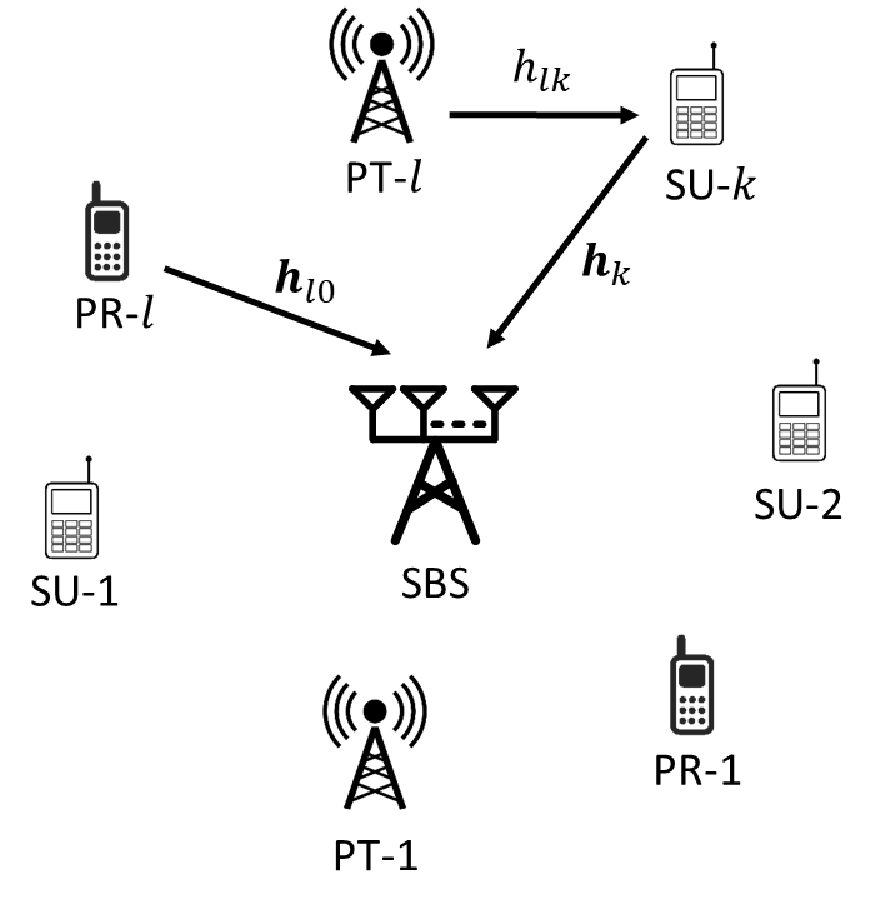
The SBS has imperfect knowledge of the channels $\mathbf{h}_{l0},\mathbf{h}_{k}$. The estimates of channels are given by $\mathbf{\hat{h}}_{l0}=\mathbf{{h}}_{l0}+\mathbf{\Delta}_{l0}$ and $\mathbf{\hat{h}}_{k}=\mathbf{h}_{k}+\mathbf{\delta}_{k}$, respectively, where $\mathbf{\Delta}_{l0}\sim\mathcal{CN}(0,\sigma^{2}_{\Delta}\mathbf{I})$, and $\mathbf{\delta}_{k}\sim\mathcal{CN}(0,\sigma^{2}_{\delta}\mathbf{I})$ are the estimation errors. We model the quality of CSI between primary and secondary system using $\sigma^{2}_{\Delta}=\frac{\sigma^{2}_{w}}{P_{p}}$, while the quality of CSI within the secondary system is modeled using $\sigma^{2}_{\delta}=\frac{\sigma^{2}_{w}}{P^{0}}$, where $P_{p}$ and $P^{0}$ are transmit powers from PTs and the SBS, respectively, and $\sigma^{2}_{w}$ is the noise power at the SBS and SUs [22, 23, 24]. We consider block fading where the channels remain constant for a finite coherence interval.

Let $\mathcal{S}_{0}=\{1,2,...,K\}$ be the set of all SUs and $\mathcal{S}\subseteq\mathcal{S}_{0}$ be the set of SUs considered for downlink transmission and $P_{k},k\in\mathcal{S}$ be the power allocated to SU-$k$ in the downlink when set ${\mathcal{S}}$ is selected. The ZF transmit vector for SU-$k$ depends on $\mathcal{S}$ and is denoted by $\mathbf{v}^{\mathcal{S}}_{k}\in{\mathbb{C}^{M\times 1}},k\in\mathcal{S}$. The unit-norm ZF vectors are computed using [19]:

where $\mathcal{S}(i)$ is the $i$-th entry in $\mathcal{S}$, and $[\mathbf{A}]_{i}$ is the $i$-th column of matrix $\mathbf{A}$. In the above equation, the matrix $\mathbf{G}_{\mathcal{S}}\in\mathbb{C}^{M\times(|\mathcal{S}|+L)}$ indicates the channel between SUs in set $\mathcal{S}$, PUs and the SBS. It should be noted that the ZF vector $\mathbf{v}^{\mathcal{S}}_{k}$ is in the null-space of the estimated channels to SU-$j,j\in\mathcal{S},j\neq k$. It is also in the null-space of the estimated channels to PRs. Therefore, $\mathbf{v}^{\mathcal{S}}_{k}$ satisfies $\mathbf{\hat{h}}^{H}_{j}\mathbf{v}^{\mathcal{S}}_{k}=0,j,k\in\mathcal{S},j\neq k$ and $\mathbf{\hat{h}}^{H}_{l0}\mathbf{v}^{\mathcal{S}}_{k}=0,l\in\mathcal{R}$.

The ZF beamforming vectors are not in the null-space of the true channel $\mathbf{h}^{H}_{l0}$ when the channel estimation error $\mathbf{\Delta}_{l0}$ is non-zero. Therefore, the interference caused at PR-$l,l\in\mathcal{R}$ is non-zero and can be expressed as:

where $I_{kl}$ is the interference contribution of data stream of SU-$k$ towards PR-$l$. The interference $I_{l}$ depends on power allocation as well as the set of SUs selected. Similarly, the inter-SU interference at SU-$k$ due to the signal transmitted toward SU-$j$ can be expressed as

Finally, the reverse interference at SU-$k$ is the sum of powers received from PTs: $I_{k}=\sum\limits_{l\in\mathcal{T}}P_{p}|{h_{lk}}|^{2}$, where $P_{p}$ is the power transmitted by PT-$l$.

Our goal is to select the maximum number of SUs for downlink transmission in order to satisfy specific instantaneous rate of $R^{0}_{k}$ to selected SUs, while keeping the interference towards PRs below $I^{0}$. The total available power at the SBS is $P^{0}$. Note that the estimated interference to PR-$l,l\in\mathcal{R}$ based on the estimated channel is $\hat{I}_{l}=\sum_{k\in\mathcal{S}}P_{k}|\mathbf{\hat{h}}^{H}_{l0}\mathbf{v}^{\mathcal{S}}_{k}|^{2}=0$. Since the true interference $I_{l}$ is non-zero, we add a margin parameter $\epsilon_{1}$ to define $\tilde{I}_{l}=\sum_{k\in\mathcal{S}}P_{k}(|\mathbf{\hat{h}}^{H}_{l0}\mathbf{v}^{\mathcal{S}}_{k}|^{2}+\epsilon_{1})$ as the new estimated value of the interference with margin.

Further, the instantaneous rate achieved at SU-$k$, when a set $\mathcal{S}$ is selected, is

where $\sigma^{2}_{w}$ is the noise power at the SU. Due to ZF beamforming, the estimated inter-SU interference will be zero, i.e., $\hat{I}_{jk}=P_{j}|\mathbf{\hat{h}}^{H}_{k}\mathbf{v}^{\mathcal{S}}_{j}|^{2}=0$ due to $\mathbf{\hat{h}}^{H}_{k}\mathbf{v}^{\mathcal{S}}_{j}=0,k\neq j$. We use a margin parameter $\epsilon_{2}$ to compensate for the estimation error in the channels between SBS and SUs. Therefore, the estimated instantaneous rate with margin becomes

Note that, unlike $I_{l}$ and $I_{jk}$, the reverse interference term $I_{k}$ can be measured at SU-$k$ by observing combined signal received from all PUs during the channel estimation phase. The optimization problem can then be formulated as follows:

Selection of parameters $\epsilon_{1}$ and $\epsilon_{2}$ is discussed in Section IV-B. By substituting $|\mathbf{\hat{h}}^{H}_{l0}\mathbf{v}^{\mathcal{S}}_{k}|^{2}=0$ and rearranging (8), we obtain the following equivalent optimization problem:

Using binary selection variables $s_{k}\in\{0,1\}$ to indicate whether SU-$k$ is selected ($s_{k}=1$) or not ($s_{k}=0$), we can restate the above problem as:

The constraint (15) is obtained by combining (11) and (13). This constraint indicates that the power allocation is controlled by the interference limit $I^{0}$ if $I^{0}/\epsilon_{1}\leq P^{0}$, while it is controlled by the transmit power limit $P^{0}$ if $I^{0}/\epsilon_{1}>P^{0}$.

As described in Section III, the power allocated to SU-$k$, $P^{\mathcal{S}_{0}}_{k}$, remains constant during the algorithmic iterations of DMP without vector update. Therefore, DMP without vector update effectively obtains the solution for the following problem:

The solution obtained by DMP without vector update can be written as follows:

The solution $\mathcal{S}^{*}_{2}$ is the optimal solution for $\mathbf{P2}$, since no set of higher cardinality can satisfy the constraint (41) for fixed $P^{\mathcal{S}_{0}}_{k}$. This is because the proposed algorithm drops the SU with the highest power allocation in each iteration until the constraint (41) is satisfied and addition of any SU to the set $\mathcal{S}^{*}_{2}$ will violate the constraint.

Further, the optimal solutions of problems $\mathbf{P1}$ and $\mathbf{P2}$ differ due to the difference in power allocations $P^{\mathcal{S}^{*}}_{k}$ and $P^{\mathcal{S}_{0}}_{k}$, where $\mathcal{S}^{*}$ indicates the optimal solution set for $\mathbf{P1}$. The power allocations differ due to the difference in the number of nulls in the ZF vectors $\mathbf{v}^{\mathcal{S}^{*}}_{k}$ and $\mathbf{v}^{\mathcal{S}_{0}}_{k}$, which are denoted by $M-|\mathcal{S}^{*}|-L+1$ and $M-K-L+1$, respectively. The difference in the power allocations $P^{\mathcal{S}^{*}}_{k}$ and $P^{\mathcal{S}_{0}}_{k}$ becomes negligible if $M\gg K+L$. From Theorem 1, we can also observe that the distribution of $P^{\mathcal{S}^{*}}_{k}$ approaches that of $P^{\mathcal{S}_{0}}_{k}$ as $\gamma^{\mathcal{S}^{*}}_{k}\rightarrow\gamma^{\mathcal{S}_{0}}_{k}$, which occurs if $M\gg K+L$. Therefore, we can conclude that the problem $\mathbf{P1}$ becomes equivalent to $\mathbf{P2}$ for $M\gg K+L$ and $|\mathcal{S}^{*}_{2}|$ approaches the optimal solution $|\mathcal{S}^{*}|$.

Finally, the number of SUs selected by the DMP algorithm is no less than the number of SUs selected by DMP without vector update, i.e, $|\mathcal{S}_{2}^{*}|\leq|\mathcal{S}_{1}^{*}|\leq|\mathcal{S}^{*}|$. This is because the power allocated to each SU in DMP is less that or equal to that in DMP without vector update, i.e., $P^{\mathcal{S}}_{k}\leq P^{\mathcal{S}_{0}}_{k}$ when a set $\mathcal{S}$ is selected. This can also be observed from Corollary 2. The condition for selection of a set $\mathcal{S}$ under DMP $\left(\sum\limits_{k\in\mathcal{S}}P^{\mathcal{S}}_{k}\leq\min\left(\frac{I^{0}}{\epsilon_{1}},P^{0}\right)\right)$ is always satisfied if the condition under DMP without vector update is satisfied $\left(\sum\limits_{k\in\mathcal{S}}P^{\mathcal{S}_{0}}_{k}\leq\min\left(\frac{I^{0}}{\epsilon_{1}},P^{0}\right)\right)$, while the converse is not true. Therefore, we get $|\mathcal{S}_{2}^{*}|\leq|\mathcal{S}_{1}^{*}|\leq|\mathcal{S}^{*}|$. This phenomenon can be intuitively explained as follows. When the set $\mathcal{S}_{0}$ is selected initially, the number of degrees of freedom in the beamforming, after adding $L+K-1$ nulls, is $M-K-L+1$. The number of degrees of freedom increments if the ZF vectors are updated after dropping an SU. Therefore, the power requirements of SUs which are not dropped reduce as the ZF vectors $\mathbf{v}_{k}$ are better aligned with channels $\mathbf{\hat{h}}_{k}$. The reduction in power requirements implies that more SUs can be kept in the downlink, while satisfying the constraints of the problem $\mathbf{P1}$. Therefore, the number of SUs selected by the DMP is no less than the number of SUs selected by DMP without vector update.

The optimization framework $\mathbf{P1}$ in (14)-(17) involves various parameters. In this section, we provide discussion on the selection of these parameters. The parameters can be broadly classified into two categories: 1) network dependent fixed parameters: $P^{0},I^{0},R^{0}_{k}$, and 2) proposed margin parameters: $\epsilon_{1},\epsilon_{2}$.

References

- [1] J. Andrews, S. Buzzi, W. Choi, S. Hanly, A. Lozano, A. Soong, and J. Zhang, “What Will 5G Be?” IEEE J. Sel. Areas Commun., vol. 32, no. 6, pp. 1065–1082, Jun. 2014.
- [2] F. Boccardi, R. Heath, A. Lozano, T. Marzetta, and P. Popovski, “Five disruptive technology directions for 5G,” IEEE Commun. Mag., vol. 52, no. 2, pp. 74–80, Feb. 2014.
- [3] A. Gupta and R. K. Jha, “A Survey of 5G Network: Architecture and Emerging Technologies,” IEEE Access, vol. 3, pp. 1206–1232, 2015.
- [4] H. Ngo, E. Larsson, and T. Marzetta, “The Multicell Multiuser MIMO Uplink with Very Large Antenna Arrays and a Finite-Dimensional Channel,” IEEE Trans. Commun., vol. 61, no. 6, pp. 2350–2361, Jun. 2013.
- [5] E. Biglieri, A. Goldsmith, L. Greenstein, N. Mandayam, and H. Poor, Principles of Cognitive Radio. Cambridge University Press, 2012.
- [6] S. Chaudhari and D. Cabric, “Feasibility of serving K secondary users in underlay cognitive radio networks using massive MIMO,” in ITG International Conf. on Systems, Commun., and Coding (SCC), Feb. 2017.
- [7] S. Yiu, C.-B. Chae, K. Yang, and D. Calin, “Uncoordinated Beamforming for Cognitive Networks,” IEEE Trans. Commun., vol. 60, no. 5, pp. 1390–1397, May 2012.
- [8] H. Du, T. Ratnarajah, M. Pesavento, and C. Papadias, “Joint Transceiver Beamforming in MIMO Cognitive Radio Network Via Second-Order Cone Programming,” IEEE Trans. Signal Process., vol. 60, no. 2, pp. 781–792, Feb. 2012.
- [9] H. Du and T. Ratnarajah, “Robust Utility Maximization and Admission Control for a MIMO Cognitive Radio Network,” IEEE Trans. Veh. Technol., vol. 62, no. 4, pp. 1707–1718, May 2013.
- [10] C. Tsinos and K. Berberidis, “Blind Opportunistic Interference Alignment in MIMO Cognitive Radio Systems,” IEEE J. Emerging and Selected Topics in Circuits and Syst., vol. 3, no. 4, pp. 626–639, Dec. 2013.
- [11] Y. Noam and A. Goldsmith, “Blind Null-Space Learning for MIMO Underlay Cognitive Radio with Primary User Interference Adaptation,” IEEE Trans. Wireless Commun., vol. 12, no. 4, pp. 1722–1734, Apr. 2013.
- [12] Y. Noam, A. Manolakos, and A. J. Goldsmith, “Null Space Learning With Interference Feedback for Spatial Division Multiple Access,” IEEE Trans. Wireless Commun., vol. 13, no. 10, pp. 5699–5715, Oct. 2014.
- [13] L. Wang, H. Ngo, M. Elkashlan, T. Duong, and K. Wong, “Massive MIMO in Spectrum Sharing Networks: Achievable Rate and Power Efficiency,” IEEE Syst. Journal, vol. PP, no. 99, pp. 1–12, 2015.
- [14] M. H. Al-Ali and K. C. Ho, “Transmit Precoding in Underlay MIMO Cognitive Radio With Unavailable or Imperfect Knowledge of Primary Interference Channel,” IEEE Trans. Wireless Commun., vol. 15, no. 8, pp. 5143–5155, Aug. 2016.
- [15] W. Xiong, A. Mukherjee, and H. M. Kwon, “MIMO Cognitive Radio User Selection With and Without Primary Channel State Information,” IEEE Trans. Veh. Technol., vol. 65, no. 2, pp. 985–991, Feb. 2016.
- [16] S. Chaudhari and D. Cabric, “Downlink transceiver beamforming and admission control for massive MIMO cognitive radio networks,” in Asilomar Conference on Signals, Systems and Computers, Nov. 2015, pp. 1257–1261.
- [17] T. Yoo and A. Goldsmith, “On the optimality of multiantenna broadcast scheduling using zero-forcing beamforming,” IEEE J. Sel. Areas Commun., vol. 24, no. 3, pp. 528–541, Mar. 2006.
- [18] S. Huang, H. Yin, J. Wu, and V. C. M. Leung, “User Selection for Multiuser MIMO Downlink With Zero-Forcing Beamforming,” IEEE Trans. Veh. Technol., vol. 62, no. 7, pp. 3084–3097, Sep. 2013.
- [19] S. Huang, H. Yin, H. Li, and V. C. M. Leung, “Decremental User Selection for Large-Scale Multi-User MIMO Downlink with Zero-Forcing Beamforming,” IEEE Wireless Commun. Lett., vol. 1, no. 5, pp. 480–483, Oct. 2012.
- [20] T. V. Chien, E. Björnson, and E. G. Larsson, “Joint Power Allocation and User Association Optimization for Massive MIMO Systems,” IEEE Trans. Wireless Commun., vol. 15, no. 9, pp. 6384–6399, Sep. 2016.
- [21] T. Marzetta, “Noncooperative Cellular Wireless with Unlimited Numbers of Base Station Antennas,” IEEE Trans. Wireless Commun., vol. 9, no. 11, pp. 3590–3600, Nov. 2010.
- [22] P. Aquilina and T. Ratnarajah, “Performance Analysis of IA Techniques in the MIMO IBC With Imperfect CSI,” IEEE Trans. Commun., vol. 63, no. 4, pp. 1259–1270, Apr. 2015.
- [23] S. M. Razavi and T. Ratnarajah, “Performance Analysis of Interference Alignment Under CSI Mismatch,” IEEE Trans. Veh. Technol., vol. 63, no. 9, pp. 4740–4748, Nov. 2014.
- [24] J. Maurer, J. Jalden, D. Seethaler, and G. Matz, “Vector Perturbation Precoding Revisited,” IEEE Trans. Signal Process., vol. 59, no. 1, pp. 315–328, Jan. 2011.
- [25] K. Hosseini, W. Yu, and R. Adve, “Large-Scale MIMO Versus Network MIMO for Multicell Interference Mitigation,” IEEE. J. Sel. Topics in Signal Process., vol. 8, no. 5, pp. 930–941, Oct. 2014.
- [26] Federal Communication Commission, Amendment of the Commission’s Rules with Regard to Commercial Operations in the 3550-3650 MHz Band. REPORT AND ORDER AND SECOND FURTHER NOTICE OF PROPOSED RULEMAKING 15-47, 2015.
- [27] Y. Ye, D. Wu, Z. Shu, and Y. Qian, “Overview of LTE Spectrum Sharing Technologies,” IEEE Access, vol. 4, pp. 8105–8115, 2016.
- [28] H. Q. Ngo, E. Larsson, and T. Marzetta, “Energy and Spectral Efficiency of Very Large Multiuser MIMO Systems,” IEEE Trans. Commun., vol. 61, no. 4, pp. 1436–1449, Apr. 2013.
- [29] C. A. Coelho and B. C. Arnold, “On the Exact and Near-Exact Distributions of the Product of Generalized Gamma Random Variables and the Generalized Variance,” Communications in Statistics - Theory and Methods, vol. 43, no. 10-12, pp. 2007–2033, 2014.
- [30] A. Leaon-Garcia, Probability and Random Processes for Electrical Engineering, 3rd ed. Addison-Wesley Publishing Company, 2008.