Model input and output dimension reduction using Karhunen Loève expansions with application to biotransport
Abstract
We consider biotransport in tumors with uncertain heterogeneous material properties. Specifically, we focus on the elliptic partial differential equation (PDE) modeling the pressure field inside the tumor. The permeability field is modeled as a log-Gaussian random field with a prespecified covariance function. We numerically explore dimension reduction of the input parameter and model output. Truncated Karhunen–Loève (KL) expansions are used to decompose the log-permeability field, as well as the resulting random pressure field. We find that although very high-dimensional representations are needed to accurately represent the permeability field, especially in presence of small correlation lengths, the pressure field is not very sensitive to high-order KL terms of the input parameter. Moreover, we find that the pressure field itself can be represented accurately using a KL expansion with a small number of terms. These observations are used to guide a reduced-order modeling approach to accelerate computational studies of biotransport in tumors.
1 INTRODUCTION
We focus on modeling biotransport processes in tumors with uncertain heterogeneous material properties. An improved understanding of these processes can provide vital insight for agent delivery in cancer treatment [1, 2]. Biotransport processes in tumors can be modeled as flows in heterogeneous porous media. Equations governing biotransport consist of an elliptic PDE describing the pressure distribution and a hyperbolic PDE that describes agent (e.g., drug) delivery in porous media [3]. The uncertain tumor material properties can be modeled as random fields, which are then incorporated as coefficient functions in the governing PDEs.
In the present work, the uncertain permeability field is modeled as a log-Gaussian random field. Our aim is to efficiently simulate the uncertain pressure field. We use KL expansions [4, 5] to represent the random log-permeability field. The use of KL expansions for representing random field parameters in mathematical models has been a common modeling approach in the uncertainty quantification community [6, 7, 8, 9, 10, 11, 12, 13, 14, 15]. The typical approach is to use a truncated KL expansion with enough term to ensure the average variance of the parameter field is sufficiently captured. That is, the truncation of the KL expansion is performed a priori and without taking the response of the governing equations to the random field coefficients in mind. We take a goal-oriented point of view: instead of relying on a truncated KL expansion of the log-permeability field that is computed independently of the governing PDE, we seek to retain only the KL terms that the PDE solution operator is sensitive to. This goal-oriented strategy can lead to significant input parameter dimension reduction, especially for input fields with small correlation lengths. The PDE solution—the pressure field—itself can also be represented via a truncated KL expansion. We observe that a low-rank representation of the pressure field is often afforded by a truncated KL expansion with a small number of terms. The latter is a consequence of the (often) rapid decay of the eignvalues of the model output covariance operator. Our approach guides an input and output dimension reduction strategy: a low-rank representation of the pressure field can be computed in a low-dimensional parameter space. We mention that a preliminary version of this work was presented in the conference paper [16].
This article is structured as follows. In Section 2, we recall the requisite background material on random fields and their KL expansion. In that section, we also outline a computational strategy for computing KL expansions for random fields with or without a prespefied covariance function. In Section 3, we use a model elliptic PDE in one space dimension to illustrate the components of the proposed approach. Then, in Section 4, we focus on a biotransport application problem. We present numerical results illustrating the merits of the proposed strategy. Concluding remarks are provided in Section 5.
2 BACKGROUND ON RANDOM FIELDS
Let be a probability space, where is a sample space, is an appropriate -algebra, and is a probability measure. Let , with , or , be a compact set. Let be a stochastic process [17]. From a modeling standpoint, can be used to represent uncertain parameters fields in mathematical models.
A stochastic process is called centered if for all , where . A process is called mean square continuous if
The covariance function and the corresponding correlation function of a stochastic process are, respectively, given by
We also recall the definition of the covariance operator of a stochastic process , which is given by
| (1) |
Karhunen–Loève expansion. Let be a centered mean-square continuous stochastic process, and let be the orthonormal basis of eigenvectors of its covariance operator with corresponding (non-negative) eigenvalues :
| (2) |
The process can be represented via its KL expansion [4, 5, 18, 19]:
| (3) |
where are centered mutually uncorrelated random variables with unit variance and are defined by
The convergence of the series (3) is uniform in , and is mean square in [4]. Moreover, if is a Gaussian process, convergence of the series (3) is almost sure for each ; see [4, p. 485] for further details.
Numerical computation of KL expansion. To compute the KL expansion of a stochastic process the eigenvalue problem (2) must be solved first. In the present work, we follow Nyström’s approach [20], which involves discretizing the generalized eigenvalue problem using quadrature. We describe the steps for computing KL expansions below. Further details on numerical methods for computing KL expansions can be found in [21].
When modeling random field coefficients in models, one often has access to a prespecified covariance function. On the other hand, when computing KL expansion of a random field output of a mathematical model we only have access to realizations of the model output. Let denote the random field output of model governed by PDEs. In practice, often the model uncertainties are parameterized using a random vector , in which case the random field output can be computed for specific realizations of . To compute the truncated KL expansion,
| (4) | ||||
the covariance function of needs to be approximated via sampling, resulting in an approximate covariance operator for the process. Then, the generalized eigenvalue problem will be solved using this approximate covariance operator to find (approximations to) and , . In practice, the dominant KL terms can be captured reliably, with a modest sample size, as discussed in our numerical results. We summarize the steps required for computing truncated KL expansion of the random process in Algorithm 1. In what follows, we refer to the coefficients in (4) as the KL modes.
3 MODEL 1D ELLIPTIC EQUATION WITH RANDOM COEFFICIENT FUNCTION
We let be a probability space, and for , consider the following model elliptic boundary value problem:
| (5) | ||||
In the following numerical experiments, the right hand side function is given by . We model the coefficient function as a log-Gaussian random field as follows. Let be a centered Gaussian process with covariance function,
| (6) |
We set the correlation length of the process to . Then, we set with
| (7) |
where and are the pointwise mean and variance of , respectively; we choose these parameters such that the pointwise mean and standard deviation of are and , respectively. Accordingly, we let and . 11 1 We have used the well-known formulas relating the mean and variance of a log-normal random variable , where is standard normal, to and . We consider the weak formulation of the problem (5), and use the continuous Galerkin finite element method, with linear basis functions, to solve the problem numerically.
We use a truncated KL expansion for ,
| (8) |
where are eigenpairs of the covariance operator of . Due to the Gaussianity of the process, are independent standard normal random variables. Note that the random vector
| (9) |
completely parameterizes the uncertainty in the problem (5), and its solution .
As a first illustration, we consider a fixed realization of as increases in Figure 1 (left). Note that sufficiently large is needed to capture the fluctuations of the random field. On the other hand, the corresponding PDE solution is less sensitive to the higher-order KL terms of the parameter, as seen in Figure 1 (right). This behavior is consistent with the analysis in [22], where a global sensitivity analysis formalism is used to quantify the impact of the KL terms of the log-coefficient, in an elliptic PDE, on variability in solution of the PDE.
 |
|
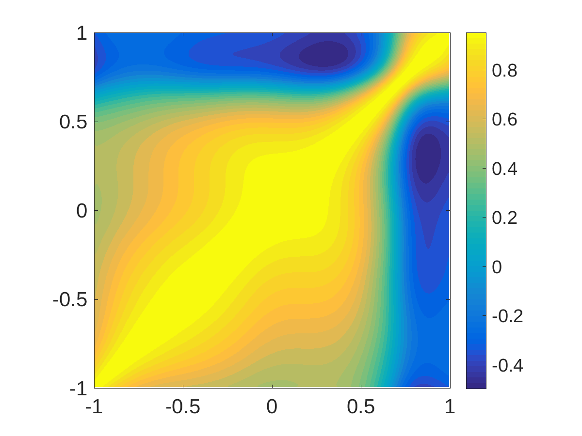
Next, we study the properties of the PDE solution . We depict the correlation function of , approximated via Monte Carlo sampling (with samples), in Figure 2 (top left). This indicates strong correlations in the output field . In Figure 2 (top right) we compare the (normalized) eigenvalues of the covariance operators for and ; we note a much faster spectral decay for the output covariance operator. The latter indicates that a KL expansion with a small number of terms can be used to approximate reasonably well. We study this by considering the KL expansion
| (10) |
of , where are the eigenpairs of covariance operator of , computed numerically using Algorithm 1, are given by
and is the mean of .
To quantify the impact of truncating the KL expansion of on its approximation properties, we study the pointwise variance with different choices of . Note also that
| (11) |
The results in Figure 2 (bottom left), indicate that pointwise variance of can be approximated well with a small . Note that the finite-element grid resolution used to solve the PDE also affects the accuracy the KL expansion of the output. In Figure 2 (bottom right) we perform a grid refinement study as we compute the pointwise variance of the process, where we fix . For the present problem using about 50 grid points seems to be sufficient to resolve the pointwise variance. More broadly, one needs a sufficiently fine computational grid to ensure the dominant eigenpairs of the covariance operator are resolved with sufficient accuracy. The grid resolution issues become more consequential in problems in two or three space dimensions, as the dimension of the discretized eigenvalue problem can become quite large.
We next study input parameter and output dimension reduction in Figure 3 where we show typical realizations of , for a small (top row) and a relatively large (bottom row) for various choices of (output dimension).
The numerical experiments in this section lead to the following observations: (i) it is possible to reduce parameter dimension by focusing on KL terms of the parameter that the PDE solution operator is most sensitive to; and (ii) it is possible to reduce output dimension by focusing on the dominant KL terms of the output. In the next section, we explore these notions systematically, in a more challenging problem, involving biotransport in tumors.
4 APPLICATION TO BIOTRANSPORT IN TUMORS
Governing equations and numerical setup. In this section, we study the pressure field in a tumor when a single needle injection occurs at the tumor center. A 2D model in a polar coordinate system is used to analyze the flow field. Consider the mass conservation law and Darcy’s law for steady incompressible flows in a 2D domain, ,
| (12) |
Here is the pressure, is the permeability, is the fluid dynamic viscosity, is the radial distance from a fixed origin, is the polar angle, is the radius of the tumor, and is the radius of the needle used to inject nanofluid into the tumor.
The boundary conditions for the pressure equation are specified as follows:
| (13) |
Herein, is the volume flow rate per unit length. Periodic boundary conditions are enforced in the direction. In this study, and are set to and , respectively, is , and is .
Uncertainties in permeability field. As before, let be a probability space. Following [23], the permeability field is modeled by a log-Gaussian random field, and its mode is set to , where stands for millidarcy. We assume that the log-permeability, , is given by
Here is the pointwise mean of the process, is the pointwise variance, and is a centered Gaussian process with unit pointwise variance for every . In this study, is set to , and is calculated from the definition of the mode of as . The covariance function of is expressed as , , where is the correlation length. As before, the (Gaussian) log-permeability field can be expressed with a truncated KL expansion,
| (14) |
where and are eigenpairs of the covariance operator of , and are independent standard normal random variables.


Uncertainty properties of the pressure field. Whereas the governing equation is more complex than the previously considered 1D problem, it is still an elliptic PDE and hence we observe similar behavior in terms of potential for dimension reduction. In the present example, we focus on pressure field over regions around the injection site. Specifically, we consider annular regions with inner boundary given by the inner boundary of the domain and the outer boundary specified by circles of radius mm, mm, or mm. Three sets of realizations of the permeability field (in the entire domain) and the corresponding model output (in the annular domain with mm) are presented in Figure 4. We observe that although the permeability field realizations exhibit complicated features, the fluctuations in the pressure field are mild.
We denote the covariance operator of the log-permeability field by and that of the pressure field by . In Figure 5 (top), we report the (normalized) eigenvalues of and those of , corresponding to mm, mm, and mm. First, we note that the eigenvalues of exhibit a far more rapid decay as compared to that of . Moreover, as the size of region of interest decreases, the spectral decay of becomes faster. In Figure 5 (middle), we examine the spectral decay of , as the correlation length of the log-permeability increases; for this test we used mm. As expected, increasing the complexity of the input parameter, by using smaller correlation lengths, leads to slower spectral decay for . However, we find that even with mm, about of average output variance is captured by the first 20 KL modes of the output. Finally, Figure 5 (bottom) summarizes the effect of input and output dimensions on capturing the average variance of the output (with mm, and input parameter correlation length mm). Note that the variance of , restricted to the region of interest, is computed by . We note that the average variance can be approximated with reasonable accuracy with small and .
We also examine the average relative error of the truncated KL representation of the output (with mm) as and increase, for input (i.e., permeability) fields with different correlation lengths; the results are reported in top and bottom panels of Figure 6, respectively. For the figure in top, we used the KL expansion of input with terms as a reference true log-permeability field. For the figure at the bottom, we compute the relative error of the output KL representation with the PDE solution restricted to the region of interest. We note that when the input dimension is fixed, the average relative error of the output KL expansion decreases very fast when the number of output KL modes increase, and is not very sensitive to input parameter correlation length. On the other hand, for small correlation lengths, there is a notable increase in the number of input KL modes needed to represent the output accurately.

Insights into reduced-order modeling. From previous analysis, we observed that the spectrum of the output covariance operator decays very fast, even when the correlation length is small. This indicates that the output, i.e., the pressure field, can be effectively approximated by a truncated KL expansion as
| (15) |
with a small number of KL terms. The importance of this approximation is that it decouples the spatial (i.e., ) dimensions and those of the random variable . If a surrogate model, such as a polynomial chaos expansion (PCE) [5, 18] is directly used to approximate the pressure field for the purpose of uncertainty quantification [23], the PCE needs to be built for each spatial point on the computational mesh. Instead, if the approximation in (15) is used, PCE (or any other suitable surrogate model) only needs to be constructed for each KL mode , .
We evaluate the performance of the reduced-order model (ROM), i.e., (15), on recovering the probability density functions (PDFs) of pressures at different locations in the flow field. The KL expansion of output is computed using Algorithm 1. As shown in [16], a modest sample size can be used to capture the dominant modes of output KL expansion. Here, to ensure accuracy, we use samples. The input dimension is fixed at in following tests. In Figure 7, we present four points, namely, , , and , on the mesh where PDFs are constructed. The contour stands for relative standard deviation (RSD) of the pressure field. Two correlation lengths, namely, mm and mm, are tested. In both cases, the region of the quantity of interest has a outer radius of mm.
In Figure 8, we present the PDFs from the full model, which is the numerical solution of the governing equation (12), and those from the ROMs with the first KL terms, where , when is mm. We observe that although the permeability field in this case is very complex, almost all ROMs with the first 10 KL terms can reasonably recover the PDFs constructed from the corresponding full models. With the first 40 KL terms, ROMs can recover the PDFs constructed from full models with negligible discrepancy on all the four points studied. When the correlation length becomes larger, e.g., mm, the effectiveness of ROMs becomes more apparent than that with small correlation lengths. From Figure 9, we can clearly see that when equals to mm, at the point , the ROM with only the first KL mode can almost recover the PDF constructed from the full model; at the point , the ROM with the first five KL modes can capture almost all the features in the PDF.

As in the 1D model problem examined earlier, we can achieve a substantial output dimension reduction by using the ROM given by it KL expansion. However, the case for the input dimension reduction is less clear in this case. When the correlation length is small, a very high input dimension is needed to capture most of the variance in the permeability field. However, as before, the PDE solution is still not very sensitive to high-order KL modes; for instance, even with mm, we note that the average relative error falls below with an of around (see Figure 6). However, if further accuracy is required, more input KL terms need to be retained. A question arises: is there a way to find a subset of the parameter KL terms that are most influential to model output variability? In our previous work [22], a derivative-based global sensitivity approach has been established to identify unimportant input parameters, for function-valued quantities of interest such as the pressure field. The approach in [22] guides an efficient input dimension reduction strategy, by identifying the KL terms of the input that contribute most to variability of the output field.
5 CONCLUSIONS
We have studied the input and output dimension reduction of elliptic PDEs, with random field input parameters, via the truncated KL expansion technique. In this study, the covariance function of the stochastic process defining the input parameter field is given, and that of the random output is constructed via Monte Carlo sampling. From numerical experiments with both 1D and 2D elliptic PDEs, we observe that when the correlation length is small, very high-dimensional representation is needed to fully resolve the variations in the input field. However, the elliptic operator is not sensitive to high-order KL terms. As a result, the solution of the elliptic PDE only shows strong dependence to the low-order KL terms of the random input field; moreover, the eigenvalues of the solution covariance operator decay very fast. This enables a low-rank representation of the PDE solution in a low-dimensional input parameter space. We then apply these dimension reduction methods in modeling the biotransport process in tumors with uncertain material properties, and demonstrate that the pressure field can be approximated with a low-dimensional representation even for random permeability fields with small correlation lengths. The efficacy of the low-rank ROMs is verified by their capability to recover the PDFs of the pressures at different locations in the flow field.
We demonstrate in this study that the truncated KL expansion can be an effective approach to reduce the output dimensions of an elliptic PDE. This is important for uncertainty quantification of large flow problems with a huge number of spatial dimensions. Although the truncated KL expansion can also reduce the input dimensions, its effect is not apparent when the correlation length of the covariance function is small. Advanced dimension reduction methods, such as global sensitivity analysis and active subspace, need to be developed to tackle input dimension reduction. One example is our recent work on functional derivative-base global sensitivity analysis [22]. More progress will be reported in our future work.
Acknowledgments
M.L. Yu gratefully acknowledge the faculty startup support from the department of mechanical engineering at the University of Maryland, Baltimore County (UMBC).
References
- [1] Salloum, M., Ma, R., Weeks, D., and Zhu, L., 2008. “Controlling nanoparticle delivery in magnetic nanoparticle hyperthermia for cancer treatment: experimental study in agarose gel”. Int. J. Hyperthermia, 24, pp. 337–345.
- [2] Debbage, P., 2009. “Targeted drugs and nanomedicine: present and future”. Current Pharmaceutical Design, 15, pp. 153–72.
- [3] Swartz, M. A., and Fleury, M. E., 2007. “Interstitial flow and its effects in soft tissues”. Annu. Rev. Biomed. Eng., 9, pp. 229–56.
- [4] Loeve, M., 1977. Probability theory I, Vol. 45 of Graduate Texts in Mathematics. New York, Heidelberg, Berlin: Springer-Verlag.
- [5] Ghanem, R. G., and Spanos, P. D., 1991. Stochastic finite elements: a spectral approach. Springer-Verlag New York, Inc., New York, NY, USA.
- [6] Ghanem, R., 1998. “Probabilistic characterization of transport in heterogeneous media”. Computer Methods in Applied Mechanics and Engineering, 158(3), pp. 199 – 220.
- [7] Le Maître, O. P., Reagan, M. T., Najm, H. N., Ghanem, R. G., and Knio, O. M., 2002. “A stochastic projection method for fluid flow: Ii. random process”. Journal of computational Physics, 181(1), pp. 9–44.
- [8] Xiu, D., and Karniadakis, G. E., 2003. “Modeling uncertainty in flow simulations via generalized polynomial chaos”. Journal of Computational Physics, 187(1), pp. 137 – 167.
- [9] Le Maıtre, O., Knio, O., Najm, H., and Ghanem, R., 2004. “Uncertainty propagation using wiener–haar expansions”. Journal of computational Physics, 197(1), pp. 28–57.
- [10] Babuška, I., Nobile, F., and Tempone, R., 2007. “A stochastic collocation method for elliptic partial differential equations with random input data”. SIAM Journal on Numerical Analysis, 45(3), pp. 1005–1034.
- [11] Doostan, A., Ghanem, R. G., and Red-Horse, J., 2007. “Stochastic model reduction for chaos representations”. Computer Methods in Applied Mechanics and Engineering, 196(37-40), pp. 3951–3966.
- [12] Saad, G., and Ghanem, R., 2009. “Characterization of reservoir simulation models using a polynomial chaos-based ensemble kalman filter”. Water Resources Research, 45(4).
- [13] Matthies, H. G., and Keese, A., 2005. “Galerkin methods for linear and nonlinear elliptic stochastic partial differential equations”. Computer methods in applied mechanics and engineering, 194(12-16), pp. 1295–1331.
- [14] Graham, I. G., Kuo, F. Y., Nichols, J. A., Scheichl, R., Schwab, C., and Sloan, I. H., 2015. “Quasi-monte carlo finite element methods for elliptic pdes with lognormal random coefficients”. Numerische Mathematik, 131(2), pp. 329–368.
- [15] Elman, H., 2017. “Solution algorithms for stochastic galerkin discretizations of differential equations with random data”. Handbook of Uncertainty Quantification, pp. 1–16.
- [16] Alexanderian, A., Reese, W., Smith, R. C., and Yu, M., 2018. “Efficient uncertainty quantification for biotransport in tumors with uncertain material properties”. In ASME 2018 International Mechanical Engineering Congress and Exposition, American Society of Mechanical Engineers, pp. V003T04A033–V003T04A033.
- [17] Williams, D., 1991. Probability with martingales. Cambridge Mathematical Textbooks. Cambridge University Press, Cambridge.
- [18] Le Maitre, O. P., and Knio, O. M., 2010. Spectral Methods for Uncertainty Quantification With Applications to Computational Fluid Dynamics. Scientific Computation. Springer.
- [19] Smith, R. C., 2013. Uncertainty Quantification: Theory, Implementation, and Applications, Vol. 12. SIAM.
- [20] Kress, R., 2014. Linear integral equations, third ed., Vol. 82 of Applied Mathematical Sciences. Springer, New York.
- [21] Betz, W., Papaioannou, I., and Straub, D., 2014. “Numerical methods for the discretization of random fields by means of the karhunen–loève expansion”. Computer Methods in Applied Mechanics and Engineering, 271, pp. 109–129.
- [22] Cleaves, H. L., Alexanderian, A., Guy, H., Smith, R. C., and Yu, M., 2019. “Derivative-based global sensitivity analysis for models with high-dimensional inputs and functional outputs”. arXiv e-prints, Feb, p. arXiv:1902.04630.
- [23] Alexanderian, A., Zhu, L., Salloum, M., Ma, R., and Yu, M., 2017. “Investigation of biotransport in a tumor with uncertain material properties using a non-intrusive spectral uncertainty quantification method”. Journal of Biomechanical Engineering, 139(9), p. 091006.