跳到论文正文
W Papers独立论文阅读器 arXiv:1903.06159 论文正文 计算阅读时间 · 0%
引用这篇论文根据当前论文元数据生成,正式投稿前建议核对。


License: arXiv.org perpetual non-exclusive license
arXiv:1903.06159v2 [math-ph] 04 Apr 2019

qq-Racah ensemble and qq-P(E7(1)/A1(1))\left(E_{7}^{(1)}/A_{1}^{(1)}\right) Discrete Painlevé equation

Anton Dzhamay Address: Anton Dzhamay: School of Mathematical Sciences
The University of Northern Colorado
Campus Box 122
501 20th Street
Greeley, CO 80639, USA
Email address: adzham@unco.edu
and Alisa Knizel Address: Aliza Knizel: Department of Mathematics
Columbia University
New York, NY, USA
Email address: knizel@math.columbia.edu
Abstract.

The goal of this paper is to investigate the missing part of the story about the relationship between the orthogonal polynomial ensembles and Painlevé equations. Namely, we consider the qq-Racah polynomial ensemble and show that the one-interval gap probabilities in this case can be expressed through a solution of the discrete qq-P(E7(1)/A1(1))\left(E_{7}^{(1)}/A_{1}^{(1)}\right) equation. Our approach also gives a new Lax pair for this equation. This Lax pair has an interesting additional involutive symmetry structure.

Key words and phrases: 
Gap probabilities, orthogonal polynomial ensembles, Askey-Wilson scheme, Painlevé equations, difference equations, isomonodromic transformations, birational transformations
2010 Mathematics Subject Classification
33D45, 34M55, 34M56, 14E07, 39A13

1. Introduction

The present paper is a continuation of the work on the relationship between the orthogonal polynomial ensembles and Painlevé equations [Kni16], where the qq-analogue of methods introduced by Arinkin and Borodin in [AB06] was developed. This relationship in the continuous settings was first established in the 90’s [TW94, HS99, WF00, BD02]. First results in the discrete case were obtained in a paper by Borodin and Boyarchenko [BB03] using the formalism of discrete integrable operators and discrete Riemann-Hilbert problems. That paper will be the starting point of our investigation.

Our goal is to establish a certain recurrence procedure for computing the so-called gap probability function for the qq-Racah orthogonal polynomial ensemble and to show that this function can be expressed through a solution of a qq-P(E7(1)/A1(1))\left(E_{7}^{(1)}/A_{1}^{(1)}\right) discrete Painlevé equation, as written in [KNY17]. For us, the original motivation to study this ensemble comes from its relationship to an interesting tiling model that we describe next.

1.1. The qq-Racah tiling model

3322221111aabbcciijj
Figure 1. A tiling of a 4×3×34\times 3\times 3 hexagon

Consider a hexagon, drawn on a regular triangular lattice, whose side lengths are given by integers a,b,c≥1a,b,c\geq 1, see Figure 1. We are interested in random tilings of such a hexagon by rhombi, also called lozenges, that are obtained by gluing two neighboring triangles together. There are three types of rhombi that arise in such a way: , , and , and so, as can be clearly seen in Figure 1, this model also has a natural interpretation as a random stepped surface formed by a stack of boxes or, equivalently, as a boxed plane partition (that is also called a 33-D Young diagram). In this way we can associate a tiling with a height function hh that assigns to every lattice vertex inside the hexagon its “height” above the “horizontal plane”, as shown on Figure 1.

We are interested in the probability measures on the set of such tilings that were introduced in [BGR10]. These probability measures form a two-parameter family generalization of the uniform distribution. If we denote these parameters by qq and κ\kappa, the weight of a tiling is defined to be the product of simple factors w⁡(      i,j)=(κ​qj−(c+1)/2−q−j+(c+1)/2/κ)w(\hbox to15.18pt{\vbox to8.94pt{\pgfpicture\makeatletter\hbox{\hskip 0.2pt\lower-4.46794pt\hbox to0.0pt{\lxSVG@begingroup@{_scopebegin} \lxSVG@begingroup@{stroke} \lxSVG@begingroup@{fill} \lxSVG@setlinewidth{\the\pgflinewidth}\lxSVG@begingroup@{stroke-width} \lx@inpgf@ignorespaces\nullfont\hbox to0.0pt{\lxSVG@begingroup@{_scopebegin} {{\lx@inpgf@ignorespaces}} {}{}{}{}{{}}{}{}{}{} {}{}{}{}{} {}{}{}{}{} {}{} {\lx@inpgf@ignorespaces}\lxSVG@begingroup@{_scopebegin} \lxSVG@begingroup@{fill} \lxSVG@begingroup@{stroke} {}\lxSVG@fillstroke\lxSVG@drawpath@unclipped{M 0 0 L 10.23 -5.91 L 20.46 0 L 10.23 5.91 Z}{} \lx@inpgf@ignorespaces \lxSVG@closescope \lxSVG@closescope {\lx@inpgf@ignorespaces}{\lx@inpgf@ignorespaces}{\lx@inpgf@ignorespaces}\hss}\lxSVG@discardpath\lxSVG@closescope \hss}}\lxSVG@closescope\endpgfpicture}}_{i,j})=(\kappa q^{j-(c+1)/2}-q^{-j+(c+1)/2}/\kappa) over all horizontal rhombi , where (i,j)(i,j) is the coordinate of the topmost point of the rhombus (the ii and jj axes are shown on Figure 1). The dependence of the factors on the location of the lozenge makes the model inhomogeneous. In order to define a probability measure, the weight of a tiling has to be non-negative. This imposes certain restrictions on the parameters qq and κ\kappa that we discuss in Section 2.

An important observation is that each lozenge tiling can be considered as time-dependent configuration of points on the line. To make this connection, we perform a simple affine transformation of the hexagon to get the shifted hexagon and the new coordinates (x,t)(x,t) as shown in Figure 2. Then each tiling naturally corresponds to a family of N=aN=a non-intersecting up-right paths (formed by the midlines of the tiles of the first two types). For each 0≤t≤b+c0\leq t\leq b+c we draw a vertical line through the point (t,0)(t,0) and denote by

x1t<x2t<⋯<xNtx^{t}_{1}<x^{t}_{2}<\cdots<x^{t}_{N}

the points of intersection of the line with the NN up-right paths. In this way, we can view a tiling as an NN-point configuration, which varies in time. Define the gap probability function on a slice tt as

(1.1) Dt​(s)=Prob​(xNt<s);D_{t}(s)=\textup{Prob}\left(x^{t}_{N}<s\right);

this function is the main object of our study.

ttxxt=3t=3
Figure 2. Modified hexagon and corresponding up-right path configuration. The dots represent the particles at time t=3t=3 and we have x1t=0x^{t}_{1}=0, x2t=2x^{t}_{2}=2, and x3t=4.x^{t}_{3}=4.

In the same way the Hahn orthogonal polynomial ensemble arises in the analysis of uniform lozenge tilings, our measures are related to the qq-Racah orthogonal polynomials. In this sense, the model goes all the way up to the top of the Askey scheme [KLS10]. The correspondence goes as follows: for a fixed section t,t, configurations x1t<x2t<⋯<xNtx^{t}_{1}<x^{t}_{2}<\cdots<x^{t}_{N} form an NN-point process. Under a suitable change of variables this point process has the same distribution as the qq-Racah orthogonal polynomial ensemble for a set of parameters that depend on the location of the vertical slice and the size of the hexagon. We elaborate more on this connection in Section 2.

An interesting aspect of this two-parameter family of probability measures is its various degenerations. For example, the uniform measure on tilings is recovered in the limit κ→0\kappa\rightarrow 0 and q→1q\rightarrow 1. Other interesting degenerations include κ→0\kappa\rightarrow 0, in which case the weight becomes proportional to q−Vq^{-V}, where VV is the number of boxes in the 33-D interpretation). On one hand, these limits correspond to some arrows in the degeneration cascades in the Askey scheme of hypergeometric and basic hypergeometric orthogonal polynomials. On the other hand, they seem to correspond to the degeneration cascades in Sakai’s classification scheme of discrete Painlevé equations [Sak01], as shown in Figure 3. Specifically, in [BB03] it was shown that gap probabilities of the form (1.1) for many examples of discrete orthogonal polynomial ensembles can be computed using a certain recurrence procedure that is essentially equivalent to the difference and qq-difference discrete Painlevé equations; some cases are labeled on Figure 3. This correspondence has been extended in [Kni16] to the qq-Hahn case that corresponds to the qq-P(E6(1)/A2(1))\left(E_{6}^{(1)}/A_{2}^{(1)}\right) discrete Painlevé equation. The qq-Racah case considered in the present paper corresponds to the qq-P(E7(1)/A1(1))\left(E_{7}^{(1)}/A_{1}^{(1)}\right) discrete Painlevé equation. Although we do not study these degenerations in detail (we plan to consider this question separately), in Section 4 we show that the weight degeneration from the qq-Racah case to the qq-Hahn case is completely consistent with the degeneration of the A1(1)A_{1}^{(1)} surface (with E7(1)E_{7}^{(1)} symmetry) into the A2(1)A_{2}^{(1)} surface (with E6(1)E_{6}^{(1)} symmetry) in Sakai’s approach.

(E8(1))e\left(E_{8}^{(1)}\right)^{e}(A1(1))|α|2=8q\left(A_{1}^{(1)}\right)^{q}_{|\alpha|^{2}=8}(E8(1))q\left(E_{8}^{(1)}\right)^{q}(E7(1))q\left(E_{7}^{(1)}\right)^{q}(E6(1))q\left(E_{6}^{(1)}\right)^{q}(D5(1))q\left(D_{5}^{(1)}\right)^{q}(A4(1))q\left(A_{4}^{(1)}\right)^{q}((A2+A1)(1))q\left((A_{2}+A_{1})^{(1)}\right)^{q}((A1+A1)(1))q\left((A_{1}+A_{1})^{(1)}\right)^{q}|α|2=14|\alpha|^{2}=14(A1(1))q\left(A_{1}^{(1)}\right)^{q}|α|2=4|\alpha|^{2}=4(A0(1))q\left(A_{0}^{(1)}\right)^{q}(E8(1))δ\left(E_{8}^{(1)}\right)^{\delta}(E7(1))δ\left(E_{7}^{(1)}\right)^{\delta}(E6(1))δ\left(E_{6}^{(1)}\right)^{\delta}(D4(1))c,δ\left(D_{4}^{(1)}\right)^{c,\delta}(A3(1))c,δ\left(A_{3}^{(1)}\right)^{c,\delta}(2​A1(1))c,δ\left(2A_{1}^{(1)}\right)^{c,\delta}(A1(1))c,δ\left(A_{1}^{(1)}\right)^{c,\delta}(A0(1))c\left(A_{0}^{(1)}\right)^{c}(2​A1(1))c,δ\left(2A_{1}^{(1)}\right)^{c,\delta}(A1(1))c,δ\left(A_{1}^{(1)}\right)^{c,\delta}(A0(1))c\left(A_{0}^{(1)}\right)^{c}qq-Racahqq-HahnRacahHahnqq-KrawtchoukLittle qq-JacobiMeixnerKrawtchoukCharlierq-PVIP_{\text{VI}}q-PVP_{\text{V}}q-PIVP_{\text{IV}}, q-PIIIP_{\text{III}}q-PIP_{\text{I}}PVIP_{\text{VI}},​ d-PVP_{\text{V}}PVP_{\text{V}},​ d-PIVP_{\text{IV}}d-PIIIP_{\text{III}}PIIIP_{\text{III}}alt.​ d-PIIP_{\text{II}}PIIIP_{\text{III}}PIIIP_{\text{III}}PIVP_{\text{IV}},​ d-PIIP_{\text{II}}PIIP_{\text{II}},​ alt.d-PIP_{\text{I}}PIP_{\text{I}}
Figure 3. The degeneration cascade for the symmetry-type classification of Painlevé equations
Refer to caption
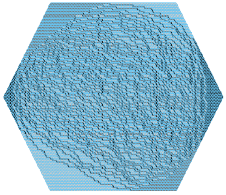
Figure 4. A simulation of a tiling for a hexagon with the sides a=60a=60, b=80b=80, c=60c=60 and parameters κ2=0,001,\kappa^{2}=0,001, q=0.995.q=0.995.

We also want to point out that the qq-Racah tiling model is a source of rich and interesting structures that are worth investigating. In particular, the asymptotic behavior of the height function of the qq-Racah tiling model when the sides of the hexagon become large and simultaneously q→1,κ→κ0q\rightarrow 1,\kappa\rightarrow\kappa_{0}, where κ0∈(0,1)\kappa_{0}\in(0,1) is fixed, was studied in [DK17], (see Figure 4 for a sample tiling in this case), where it was proved that there exists a deterministic limit shape h^\hat{h} and the random height functions hh concentrate near it with high probability as the parameters of the model scale to their critical values. An important feature of that model is that the limit shape develops frozen facets where the height function is linear. In addition, the frozen facets are interpolated by a connected disordered liquid region. In terms of the tiling, a frozen facet corresponds to a region where asymptotically only one type of lozenge is present, and in the liquid region one sees lozenges of all three types, see Figure 4. Similar concentration phenomena for the random height function in the case of the uniform measure and the measure proportional to q−Vq^{-V} are well-understood. In particular, in these cases convergence of the random height function to a deterministic function for a large class of domains was established in [JPS98, CKP01, Des98, DMB97, KO07].

The results of the present paper predict the appearance of the Painlevé transcendents in the limit regime for the fluctuations of the height function near the boundary of the limit shape.

1.2. Moduli spaces of qq-connections

Our approach is based on the ideas introduced in [BB03] and [AB06]. First, using Discrete Riemann-Hilbert Problem formalism of [Bor00, Bor03], we express the gap probability function in terms of the matrix entries of a sequence of matrices As​(z)A_{s}(z) of a certain form. We then describe the general moduli space of matrices of this form (equivalently, the moduli space of qq-connections) and show that its smallest compactification is isomorphic to a A1(1)A_{1}^{(1)}-surface in Sakai’s approach. The evolution As​(z)↦As+1​(z)A_{s}(z)\mapsto A_{s+1}(z) is given by an isomonodromy transformation that can be thought of as an isomorphism between two different surfaces in the A1(1)A_{1}^{(1)}-family, and so it is not surprising that it is given by a discrete qq-P(E7(1)/A1(1))\left(E_{7}^{(1)}/A_{1}^{(1)}\right) Painléve equation. We first identify this equation indirectly through the action of the isomonodromic dynamics on the parameters of the moduli space, and then show how to change coordinates to explicitly transform this equation into the standard form.

One new and interesting aspect of the qq-Racah case is a certain involutive symmetry of the problem. Following the ideas of D. Arinkin and A. Borodin, see also [OR17b], we formalize this involutive symmetry structure via the notion of an elliptic connection.

Definition 1.2.1.

Let ℰ\mathcal{E} be a symmetric bi-quadratic curve in ℙ1×ℙ1\mathbb{P}^{1}\times\mathbb{P}^{1} i.e., ℰ\mathcal{E} a zero locus of a symmetric bi-degree (2,2)(2,2) polynomial. Note that generically ℰ\mathcal{E} is elliptic. An ℰ\mathcal{E}-connection (or an elliptic connection) is a pair (ℒ,𝒜),(\mathcal{L},\mathcal{A}), where ℒ\mathcal{L} is a vector bundle on ℙ1\mathbb{P}^{1}, and where for any point (x,y)∈ℰ(x,y)\in\mathcal{E}, we have a map 𝒜⁡(x,y):ℒy→ℒx\mathcal{A}(x,y):\mathcal{L}_{y}\to\mathcal{L}_{x} such that 𝒜⁡(x,y)\mathcal{A}(x,y) is a rational function of (x,y)∈ℰ(x,y)\in\mathcal{E} satisfying the involutivity condition 𝒜⁡(y,x)=𝒜​(x,y)−1\mathcal{A}(y,x)=\mathcal{A}(x,y)^{-1}.

For our purposes we need to consider a degenerate case when ℰ\mathcal{E} is a nodal rational curve. Namely, let u,q∈(0,1)u,q\in(0,1) be two fixed parameters, and let the curve ℰu\mathcal{E}_{u} be given by the following equation (in the affine chart ℂ1×ℂ1⊂ℙ1×ℙ1\mathbb{C}^{1}\times\mathbb{C}^{1}\subset\mathbb{P}^{1}\times\mathbb{P}^{1}):

ℰu:(x−q​y)​(y−q​x)=u2q2​(1−q)2​(1+q).\mathcal{E}_{u}:\quad(x-qy)(y-qx)=\frac{u^{2}}{q^{2}}(1-q)^{2}(1+q).

This curve has the following rational parameterization in terms of a parameter z∈ℙ1z\in\mathbb{P}^{1}:

x⁡(z)=q−1​z+u2/z,y⁡(z)=z+u2/(q​z)=x⁡(q​z).x(z)=q^{-1}z+u^{2}/z,\quad y(z)=z+u^{2}/(qz)=x(qz).

In this way we can identify 𝒜⁡(x,y)=𝒜⁡(z)\mathcal{A}(x,y)=\mathcal{A}(z), 𝒜⁡(y,x)=𝒜⁡(u2/z)\mathcal{A}(y,x)=\mathcal{A}(u^{2}/z), and the mapping 𝒜⁡(x,y):ℒy→ℒx\mathcal{A}(x,y):\mathcal{L}_{y}\to\mathcal{L}_{x} induces the mapping 𝒜⁡(z):ℒz→ℒq​z\mathcal{A}(z):\mathcal{L}_{z}\to\mathcal{L}_{qz}. The latter mapping is the usual definition of a qq-connection, but the above formalism allows us to incorporate into it the symmetry condition.

Definition 1.2.2.

We say that a point z0∈ℙ1z_{0}\in\mathbb{P}^{1} is a pole of 𝒜\mathcal{A} if 𝒜⁡(z)\mathcal{A}(z) is not regular at z=z0z=z_{0}. We say that z0∈ℙ1z_{0}\in\mathbb{P}^{1} is a zero of 𝒜\mathcal{A} if the map 𝒜−1​(z):ℒq−1​z→ℒz\mathcal{A}^{-1}(z):\mathcal{L}_{q^{-1}z}\rightarrow\mathcal{L}_{z} is not regular at z=z0z=z_{0}. Note that 𝒜\mathcal{A} can have a zero and a pole at the same point.

Definition 1.2.3.

Suppose ℛ:ℒ→ℒ^\mathcal{R}:\mathcal{L}\rightarrow\hat{\mathcal{L}} is a rational isomorphism between two vector bundles on ℰu≃ℙ1\mathcal{E}_{u}\simeq\mathbb{P}^{1}. We say that ℒ^\hat{\mathcal{L}} is a modification of ℒ\mathcal{L} on a finite set S⊂ℰuS\subset\mathcal{E}_{u} if ℛ⁡(z)\mathcal{R}(z) and ℛ−1​(z)\mathcal{R}^{-1}(z) are regular outside SS. We call ℒ^\hat{\mathcal{L}} an upper modification of ℒ\mathcal{L} if ℛ\mathcal{R} is regular (then ℒ\mathcal{L} is called a lower modification of ℒ^\hat{\mathcal{L}}). A ℰu\mathcal{E}_{u}-connection (ℒ,𝒜⁡(z))(\mathcal{L},\mathcal{A}(z)) induces a ℰu\mathcal{E}_{u}-connection (ℒ^,𝒜^​(z))(\hat{\mathcal{L}},\hat{\mathcal{A}}(z)) that we also call a modification of (ℒ,𝒜⁡(z))(\mathcal{L},\mathcal{A}(z)).

A class of ℰu\mathcal{E}_{u}-connections that we consider depends on 88 complex parameters (z1,z2,z3,z4,z5,z6,d1,d2)(z_{1},z_{2},z_{3},z_{4},z_{5},z_{6},d_{1},d_{2}). After choosing a trivialization of ℒ\mathcal{L} over the affine chart ℂ⊂ℙ1\mathbb{C}\subset\mathbb{P}^{1}, the matrix A⁡(z)A(z) of the connection 𝒜\mathcal{A} has the following form (see Section 3):

A⁡(z)=1P⁡(z)​[b11​(z)b12​(z)zb21​(z)b22​(z)],b21​(0)=0,A(z)=\frac{1}{P(z)}\begin{bmatrix}b_{11}(z)&\frac{b_{12}(z)}{z}\\ b_{21}(z)&b_{22}(z)\end{bmatrix},\quad b_{21}(0)=0,

where bi​j​(z)b_{ij}(z) are polynomials with deg⁡(b11​(z))≤6\deg(b_{11}(z))\leq 6, deg⁡(b12​(z))≤8\deg(b_{12}(z))\leq 8, deg⁡(b21​(z))≤5\deg(b_{21}(z))\leq 5, deg⁡(b22​(z))≤6\deg(b_{22}(z))\leq 6, and

detA⁡(z)=Q⁡(z)P⁡(z),P⁡(z)=(z−z1)​(z−u2/z2)​(z−z3)​(z−u2/z4)​(z−z5)​(z−u2/z6),Q⁡(z)=z1​z3​z5z2​z4​z6​(z−u2/z1)​(z−z2)​(z−u2/z3)​(z−z4)​(z−u2/z5)​(z−z6).\det A(z)=\frac{Q(z)}{P(z)},\qquad\begin{aligned} P(z)&=(z-z_{1})(z-u^{2}/z_{2})(z-z_{3})(z-u^{2}/z_{4})(z-z_{5})(z-u^{2}/z_{6}),\\ Q(z)&=\frac{z_{1}z_{3}z_{5}}{z_{2}z_{4}z_{6}}(z-u^{2}/z_{1})(z-z_{2})(z-u^{2}/z_{3})(z-z_{4})(z-u^{2}/z_{5})(z-z_{6}).\end{aligned}

We also require that A⁡(z)A(z) satisfies the asymptotic condition

S⁡(zq+u2z)​A​(z)​S−1​(z+u2q​z)∼[d100d2],whereS⁡(z)=[100z],S\left(\frac{z}{q}+\frac{u^{2}}{z}\right)A(z)S^{-1}\left(z+\frac{u^{2}}{qz}\right)\sim\begin{bmatrix}d_{1}&0\\ 0&d_{2}\end{bmatrix},\qquad\text{where}\quad S(z)=\begin{bmatrix}1&0\\ 0&z\end{bmatrix},

and the involution condition

A⁡(u2/z)=A−1​(z).A(u^{2}/z)=A^{-1}(z).

We consider A⁡(z)A(z) modulo gauge transformations of the form

A^​(z)=R⁡(zq+u2z)​A​(z)​R−1​(z+u2q​z),R⁡(z)=[r11​(z)r12​(z)0r22​(z)],\hat{A}(z)=R\left(\frac{z}{q}+\frac{u^{2}}{z}\right)A(z)R^{-1}\left(z+\frac{u^{2}}{qz}\right),\qquad R(z)=\begin{bmatrix}r_{11}(z)&r_{12}(z)\\ 0&r_{22}(z)\end{bmatrix},

where ri​j​(z)r_{ij}(z) are polynomials with deg⁡(r11​(z))=deg⁡(r22​(z))=0\deg(r_{11}(z))=\deg(r_{22}(z))=0 and deg⁡(r12​(z))≤1\deg(r_{12}(z))\leq 1.

Lemma 1.2.4.

Under certain non-degeneracy conditions on the parameters λ=(z1,z2,…,z6,d1,d2)\lambda=(z_{1},z_{2},\dots,z_{6},d_{1},d_{2}) of a ℰu\mathcal{E}_{u}-connection 𝒜,\mathcal{A}, there exits its unique modification 𝒜¯\overline{\mathcal{A}} of type λ¯=(z1,q​z2,z3,q​z4,z5,z6,q−1​d1,q−1​d2)\overline{\lambda}=(z_{1},qz_{2},z_{3},qz_{4},z_{5},z_{6},q^{-1}d_{1},q^{-1}d_{2}).

Let us assume that the parameters (z1,…,z6,d1,d2)(z_{1},\dots,z_{6},d_{1},d_{2}) are generic; the precise meaning of this condition is explained in Section 3. We show that the moduli space MλM_{\lambda} of qq-connections of type λ=(z1,z2,…,z6,d1,d2)\lambda=(z_{1},z_{2},\dots,z_{6},d_{1},d_{2}) modulo qq-gauge transformations is two-dimensional and its smallest smooth compactification can be identified with ℙ1×ℙ1\mathbb{P}^{1}\times\mathbb{P}^{1} blown-up at eight points; more precisely, it is a Sakai surface of type A1(1)A_{1}^{(1)}. We denote the parameters on this surface by (f,g),(f,g), they are described in (3.9) in terms of the usual spectral coordinates.

Theorem 1.2.5.

Consider the modification of ℒ\mathcal{L} to ℒ^\hat{\mathcal{L}} from Lemma 1.2.4 that shifts

z2→q​z2,z4→q​z4,d1→q−1​d1,d2→q−1​d2.z_{2}\rightarrow qz_{2},\quad z_{4}\rightarrow qz_{4},\quad d_{1}\rightarrow q^{-1}d_{1},\quad d_{2}\rightarrow q^{-1}d_{2}.

Then this modification defines a regular morphism between two moduli spaces MλM_{\lambda} and Mλ¯M_{\overline{\lambda}}. Moreover, the coordinates (f¯,g¯)(\overline{f},\overline{g}) on the moduli space Mλ¯M_{\overline{\lambda}} are related to (f,g)(f,g) by the qq-P(E7(1)/A1(1))\left(E_{7}^{(1)}/A_{1}^{(1)}\right) Painlevé equation

(1.2) {(f​g−κ1κ2)​(f¯​g−κ1q​κ2)(f​g−1)​(f¯​g−1)=(g−ν5κ2)​(g−ν6κ2)​(g−ν7κ2)​(g−ν8κ2)(g−1ν1)​(g−1ν2)​(g−1ν3)​(g−1ν4),(f​g−κ1κ2)​(f​g¯−q​κ1κ2)(f​g−1)​(f​g¯−1)=(f−κ1ν5)​(f−κ1ν6)​(f−κ1ν7)​(f−κ1ν8)(f−ν1)​(f−ν2)​(f−ν3)​(f−ν4).,\left\{\begin{aligned} \frac{\left(fg-\frac{\kappa_{1}}{\kappa_{2}}\right)(\overline{f}g-\frac{\kappa_{1}}{q\kappa_{2}})}{(fg-1)(\overline{f}g-1)}&=\frac{\left(g-\frac{\nu_{5}}{\kappa_{2}}\right)\left(g-\frac{\nu_{6}}{\kappa_{2}}\right)\left(g-\frac{\nu_{7}}{\kappa_{2}}\right)\left(g-\frac{\nu_{8}}{\kappa_{2}}\right)}{\left(g-\frac{1}{\nu_{1}}\right)\left(g-\frac{1}{\nu_{2}}\right)\left(g-\frac{1}{\nu_{3}}\right)\left(g-\frac{1}{\nu_{4}}\right)},\\ \frac{\left(fg-\frac{\kappa_{1}}{\kappa_{2}}\right)(f\underline{g}-\frac{q\kappa_{1}}{\kappa_{2}})}{(fg-1)(f\underline{g}-1)}&=\frac{\left(f-\frac{\kappa_{1}}{\nu_{5}}\right)\left(f-\frac{\kappa_{1}}{\nu_{6}}\right)\left(f-\frac{\kappa_{1}}{\nu_{7}}\right)\left(f-\frac{\kappa_{1}}{\nu_{8}}\right)}{\left(f-\nu_{1}\right)\left(f-\nu_{2}\right)\left(f-\nu_{3}\right)\left(f-\nu_{4}\right)}.\end{aligned}\right.,

where we have the following matching of parameters:

ν1=1z6,ν2=1z1,ν3=1z3,ν4=1z5,ν5=u​z4z2,ν6=u,ν7=d1​z4​z6u,ν8=d2​z4​z6u,κ1=uz2,κ2=z4u.\nu_{1}=\frac{1}{z_{6}},\,\nu_{2}=\frac{1}{z_{1}},\,\nu_{3}=\frac{1}{z_{3}},\,\nu_{4}=\frac{1}{z_{5}},\,\nu_{5}=\frac{uz_{4}}{z_{2}},\,\nu_{6}=u,\,\nu_{7}=\frac{d_{1}z_{4}z_{6}}{u},\,\nu_{8}=\frac{d_{2}z_{4}z_{6}}{u},\,\kappa_{1}=\frac{u}{z_{2}},\,\kappa_{2}=\frac{z_{4}}{u}.
Remark 1.2.6.

The form (1.2) of the standard qq-P(E7(1)/A1(1))\left(E_{7}^{(1)}/A_{1}^{(1)}\right) equation here follows the recent survey monograph [KNY17] (equation (8.7) in 8.1.3). It is given as two maps (f,g)↦(f¯,g)(f,g)\mapsto(\overline{f},g) and (f,g¯)↦(f,g)(f,\underline{g})\mapsto(f,g), which reflects the QRT origin of this equation, but it is easy to rewrite it as a mapping (f,g)↦(f¯,g¯)(f,g)\mapsto(\overline{f},\overline{g}).

We also want to point out that this equation was originally obtained by Grammaticos and Ramani [GR99] (equations (14a) and (14b)), where it is called the the asymmetric qq-PVIP_{\text{VI}} equation.

We believe that important new aspects of the present paper are the following. First, it is a good illustration of the power of Sakai’s geometric theory for applications. Here we show how from just the minimal knowledge of the singularity structure of the connection and the evolution of parameters we can identify our dynamics with the standard discrete Painlevé dynamics and produce the required non-trivial change of coordinates that significantly simplifies the further computations. On one hand, our approach is algorithmic and it is adaptable to other applications, but on the other hand it uses the full power of algebro-geometric theory of discrete Painlevé equations. Second, the qq-Racah weight that we consider is at the top of the degeneration cascade, so other models can be obtained from it through degenerations, as we showed for the qq-Hahn limit. Further, the qq-Racah case was not considered in [BB03], so we needed to adopt the computation of the gap probabilities through the discrete Riemann-Hilbert problems from [BB03] to work for this model.

Acknowledgements

The authors want to thank Dima Arinkin, Alexei Borodin, Kenji Kajiwara, and Tomoyuki Takenawa for many helpful discussions and suggestions. A part of the work was completed when the authors attended the 2017 IAS PCMI Summer Session on Random Matrices, and we are grateful to the organizers for the hospitality and support. AK was partially supported by the NSF grant DMS-1704186. AD was partially supported by the UNCO grant SSI-2018.

2. The qq-Racah Orthogonal Polynomial Ensemble

2.1. Orthogonal Polynomials

Let 𝔛\mathfrak{X} be a finite subset of ℂ\mathbb{C} such that card​(𝔛)=M+1<∞\mbox{card}(\mathfrak{X})=M+1<\infty and ω:𝔛→ℝ>0\omega:\mathfrak{X}\rightarrow\mathbb{R}_{>0} be any function. Using ω\omega as a weight function, we can define an inner product on the space ℂ⁡[z]\mathbb{C}[z] of complex polynomials via

(f,g)ω:=∑x∈𝔛f⁡(x)​g​(x)​ω​(x),f,g∈ℂ⁡[z].\left(f,g\right)_{\omega}:=\sum\limits_{x\in\mathfrak{X}}f(x)g(x)\omega(x),\quad f,g\in\mathbb{C}[z].

Given this inner product, a set {Pn}n=0M\{P_{n}\}_{n=0}^{M} of complex polynomials is called a collection of orthogonal polynomials associated to the weight function ω\omega if

  • •

    PnP_{n} is a polynomial of degree nn for all n=1,…,Mn=1,\dots,M and P0≡c​o​n​s​tP_{0}\equiv const;

  • •

    if m≠nm\neq n then (Pm,Pn)ω=0(P_{m},P_{n})_{\omega}=0.

We always take PnP_{n} to be monic, i.e. Pn​(z)=zn+lower order termsP_{n}(z)=z^{n}+\text{lower order terms}.

It is clear that a collection of orthogonal polynomials {Pn}n=0M\{P_{n}\}_{n=0}^{M} associated to ω\omega and satisfying the condition (Pn,Pn)ω≠0(P_{n},P_{n})_{\omega}\neq 0 for all n=0,…,Mn=0,\dots,M exists if and only if the restriction of (⋅,⋅)ω(\cdot,\cdot)_{\omega} to the space ℂ​[z]≤d\mathbb{C}[z]^{\leq d} of polynomials of degree at most dd is nondegenerate for all d=0,…,Md=0,\dots,M. If this condition holds we say that the weight function ω\omega is nondegenerate, and in that case it is clear that the collection {Pn}n=0M\{P_{n}\}_{n=0}^{M} (with the monic normalization) is unique.

Definition 2.1.1.

Fix N∈{1,…,M+1}.N\in\{1,\dots,M+1\}. Under the above assumptions, an NN-orthogonal discrete polynomial ensemble on 𝔛\mathfrak{X} with the weight function ω\omega is a probability distribution on NN-tuples (χ1,…,χN),(\chi_{1},\dots,\chi_{N}), χi∈𝔛,\chi_{i}\in\mathfrak{X}, that is defined by

(2.1) ℙ⁡(χ1,…,χN)=1Z⁡(N,M)​∏1≤i<j≤N(χi−χj)2⋅∏i=1Nω⁡(χi),\mathbb{P}(\chi_{1},\dots,\chi_{N})=\frac{1}{Z(N,M)}\prod_{1\leq i<j\leq N}\left(\chi_{i}-\chi_{j}\right)^{2}\cdot\prod_{i=1}^{N}{\omega(\chi_{i})},

where Z⁡(N,M)Z(N,M) is the usual normalization constant.

It is well known (see, e.g., [Joh06] or [Kö5]) that such an ensemble is a determinantal point process whose correlation kernel K⁡(x,y)K(x,y) can be written in terms of the orthogonal polynomials,

(2.2) K⁡(x,y)=ω⁡(x)​ω​(y)​∑i=0N−1Pi​(x)​Pi​(y)(Pi,Pi)ω={ω⁡(x)​ω​(y)​ϕ⁡(x)​ψ​(y)−ψ⁡(x)​ϕ​(y)x−y,x≠y,ω⁡(x)​(ϕ′​(x)​ψ​(x)−ϕ⁡(x)​ψ′​(x)),x=y,K(x,y)=\sqrt{\omega(x)\omega(y)}\sum_{i=0}^{N-1}\frac{P_{i}(x)P_{i}(y)}{(P_{i},P_{i})_{\omega}}=\begin{cases}\sqrt{\omega(x)\omega(y)}\frac{\phi(x)\psi(y)-\psi(x)\phi(y)}{x-y},&\quad x\neq y,\\ \omega(x)(\phi^{\prime}(x)\psi(x)-\phi(x)\psi^{\prime}(x)),&\quad x=y,\end{cases}

where ϕ​(z)=PN​(z)\phi(z)=P_{N}(z) and ψ⁡(z)=(PN−1,PN−1)ω−1⋅PN−1​(z)\psi(z)=(P_{N-1},P_{N-1})^{-1}_{\omega}\cdot P_{N-1}(z). The second equality here follows from the observation that K⁡(x,y)K(x,y) is equal to the product of ω⁡(x)​ω​(y)\sqrt{\omega(x)\omega(y)} with the NthN^{\text{th}} Christoffel-Darboux kernel for this system of orthogonal polynomials, see [Sze67].

Let us parametrize the set 𝔛\mathfrak{X} as 𝔛={πx}x=0M\mathfrak{X}=\{\pi_{x}\}^{M}_{x=0}, where πx<πx+1,\pi_{x}<\pi_{x+1}, x=0,…,Mx=0,\dots,M. For any s∈ℕs\in\mathbb{N}, N≤s≤MN\leq s\leq M, let ℨs={πj}j=0s−1\mathfrak{Z}_{s}=\{\pi_{j}\}_{j=0}^{s-1} and let 𝔑s=𝔛∖ℨs={πj}j=sM\mathfrak{N}_{s}=\mathfrak{X}\setminus\mathfrak{Z}_{s}=\{\pi_{j}\}_{j=s}^{M}. It is well-known, see [BB03] or [AGZ10], that the so-called gap probabilities DsD_{s} for to this ensemble, defined below, can be expressed as a Fredholm determinant of the correlation kernel K⁡(x,y)K(x,y) given by (2.2),

Ds=Prob​(max⁡{πi}i=1N<πs)=det(1−Ks),where ​Ks=K|𝔑s×𝔑s.D_{s}=\text{Prob}\left(\max\{\pi_{i}\}_{i=1}^{N}<\pi_{s}\right)=\det(1-K_{s}),\quad\text{where }K_{s}=K|_{\mathfrak{N}_{s}\times\mathfrak{N}_{s}}.

These are the quantities that we are interested in computing.

2.1.1. qq-Racah Orthogonal Polynomial Ensemble

In this section we recall some basic properties of the qq-Racah orthogonal polynomials, cf. [KS96, Section 3.2].

Definition 2.1.2.

Let q∈(0,1),q\in(0,1), M∈ℤ≥0M\in\mathbb{Z}_{\geq 0}, α,β,γ,δ∈ℝ\alpha,\beta,\gamma,\delta\in\mathbb{R} and γ=q−M−1.\gamma=q^{-M-1}. For x=0,1,…,Mx=0,1,\ldots,M, the qq-Racah weight function ωqR​(x)\omega^{\textup{qR}}(x) is defined by

(2.3) ωqR​(x)=(α​q,β​δ​q,γ​q,γ​δ​q,q)x(q,α−1​γ​δ​q,β−1​γ​q,δ​q,q)x​(1−γ​δ​q2​x+1)(α​β​q)x​(1−γ​δ​q),\omega^{\textup{qR}}(x)=\frac{(\alpha q,\beta\delta q,\gamma q,\gamma\delta q;q)_{x}}{(q,\alpha^{-1}\gamma\delta q,\beta^{-1}\gamma q,\delta q;q)_{x}}\frac{(1-\gamma\delta q^{2x+1})}{(\alpha\beta q)^{x}(1-\gamma\delta q)},

where (y1,…,yi;q)k:=(y1;q)k⋯(yi;q)k(y_{1},\dots,y_{i};q)_{k}:=(y_{1};q)_{k}\cdots(y_{i};q)_{k} and (y;q)k:=(1−y)(1−yq)⋯(1−yqk−1)(y;q)_{k}:=(1-y)(1-yq)\cdots(1-yq^{k-1}) is the usual qq-Pochhammer symbol.

Remark 2.1.3.

The condition γ=q−M−1\gamma=q^{-M-1} can be replaced by α=q−M−1\alpha=q^{-M-1} or β​δ=q−M−1\beta\delta=q^{-M-1}. Our choice is due to the fact that under the substitutions γ=q−M−1\gamma=q^{-M-1} and δ=0\delta=0 the qq-Racah weight reduces to the qq-Hahn weight ωqH​(x)=(α​q,q−M,q)x(q,β−1​q−M,q)x​(α​β​q)x\omega^{\textup{qH}}(x)=\frac{(\alpha q,q^{-M};q)_{x}}{(q,\beta^{-1}q^{-M};q)_{x}(\alpha\beta q)^{x}}.

Definition 2.1.4.

Fix N∈ℤ≥1N\in\mathbb{Z}_{\geq 1} and let α,β,γ,δ,q\alpha,\beta,\gamma,\delta,q and MM be as in Definition 2.1.2 with M≥N−1M\geq N-1. Denote by 𝔛N\mathfrak{X}^{N} a collection of NN-tuples of non-negative integers,

𝔛N={(λ1,…,λN)∈ℤN:0≤λ1<λ2<⋯<λN≤M}.\mathfrak{X}^{N}=\{(\lambda_{1},\dots,\lambda_{N})\in\mathbb{Z}^{N}:0\leq\lambda_{1}<\lambda_{2}<\dots<\lambda_{N}\leq M\}.

The qq-Racah ensemble is a probability measure ℙqR\mathbb{P}^{\textup{qR}} on the set 𝔛N\mathfrak{X}^{N} that is given by

(2.4) ℙqR​(λ1,…,λN)=1Z⁡(N,M,α,β,γ,δ,q)​∏1≤i<j≤N(σ⁡(q−λi)−σ⁡(q−λj))2⋅∏i=1Nωq​R​(λi),\mathbb{P}^{\textup{qR}}(\lambda_{1},\dots,\lambda_{N})=\frac{1}{Z(N,M,\alpha,\beta,\gamma,\delta,q)}\prod_{1\leq i<j\leq N}\left(\sigma(q^{-\lambda_{i}})-\sigma(q^{-\lambda_{j}})\right)^{2}\cdot\prod_{i=1}^{N}{\omega^{qR}(\lambda_{i})},

where σ⁡(z)=z+γ​δ​q​z−1\sigma(z)=z+\gamma\delta qz^{-1} and Z⁡(N,M,α,β,γ,δ,q)Z(N,M,\alpha,\beta,\gamma,\delta,q) is the usual probabilistic normalization constant.

For ℙqR\mathbb{P}^{\textup{qR}} to be an actual probability measure, expressions in (2.4) have to be non-negative, and this is not necessarily the case for a generic choice of parameters. Thus, some restrictions on the space of parameters have to be imposed and we make one such possible choice in the following assumption.

Assumption 2.1.5.

We assume that parameters α,β,γ,δ,q∈ℝ\alpha,\beta,\gamma,\delta,q\in\mathbb{R} and M,N∈ℤM,N\in\mathbb{Z} are such that

M≥N−1≥0,1>q>0,α,β>0,δ≥0,γ=q−M−1,1>βδ,β≥γ,α≥γ.M\geq N-1\geq 0,\hskip 5.69054pt1>q>0,\hskip 5.69054pt\alpha,\beta>0,\hskip 5.69054pt\delta\geq 0,\hskip 5.69054pt\gamma=q^{-M-1},\hskip 5.69054pt1>\beta\delta,\hskip 5.69054pt\beta\geq\gamma,\hskip 5.69054pt\alpha\geq\gamma.

Then expressions in (2.4) are non-negative on all of 𝔛N\mathfrak{X}^{N} and indeed define a probability measure ℙqR\mathbb{P}^{\textup{qR}}.

Remark 2.1.6.

Although we chose to consider qq-Racah ensemble as a probability measure on NN-tuples of (λ1,…,λN)(\lambda_{1},\dots,\lambda_{N}), it can also be viewed as a measure on (σ⁡(q−λ1),…,σ⁡(q−λN))(\sigma(q^{-\lambda_{1}}),\dots,\sigma(q^{-\lambda_{N}})), to agree with Definition 2.1.1.

It is well known that ωqR\omega^{\textup{qR}} is a nondegenerate weight function. Orthogonal polynomials {Pn​(z)}n=0M\{P_{n}(z)\}_{n=0}^{M} associated to it are called the qq-Racah orthogonal polynomials. They satisfy the following orthogonality relation, written in the argument σ⁡(q−x):=q−x+γ​δ​qx+1\sigma(q^{-x}):=q^{-x}+\gamma\delta q^{x+1}:

(2.5) ∑x=0MωqR​(x)​Pm​(σ⁡(q−x))​Pn​(σ⁡(q−x))=cn⋅δm​n, where cn=(γ​δ​q2,α−1​β−1​γ,α−1​δ,β−1,q)∞(α−1​γ​δ​q,β−1​γ​q,δ​q,α−1​β−1​q−1,q)∞​(1−α​β​q)​(γ​δ​q)n(1−α​β​q2​n+1)​(q,β​q,α​δ−1​q,α​β​γ−1​q,q)n(α​β​q,α​q,β​δ​q,γ​q,q)n.\begin{split}&\sum_{x=0}^{M}\omega^{\textup{qR}}(x)P_{m}\left(\sigma(q^{-x})\right)P_{n}\left(\sigma(q^{-x})\right)=c_{n}\cdot\delta_{mn},\mbox{ where }\\ &c_{n}=\frac{(\gamma\delta q^{2},\alpha^{-1}\beta^{-1}\gamma,\alpha^{-1}\delta,\beta^{-1};q)_{\infty}}{(\alpha^{-1}\gamma\delta q,\beta^{-1}\gamma q,\delta q,\alpha^{-1}\beta^{-1}q^{-1};q)_{\infty}}\frac{(1-\alpha\beta q)(\gamma\delta q)^{n}}{(1-\alpha\beta q^{2n+1})}\frac{(q,\beta q,\alpha\delta^{-1}q,\alpha\beta\gamma^{-1}q;q)_{n}}{(\alpha\beta q,\alpha q,\beta\delta q,\gamma q;q)_{n}}.\end{split}

A connection between qq-Racah ensemble and the tiling model described in Section 1.1 is given by the following Theorem, see [BGR10].

Theorem 2.1.7.

Consider the tiling of a hexagon with side lengths a,b,ca,b,c. Let N=a,T=b+c,S=cN=a,T=b+c,S=c, and let q∈(0,1)q\in(0,1), κ∈[0,q(T−1)/2)\kappa\in\left[0,q^{(T-1)/2}\right). Fix t∈{0,1,…,T}t\in\{0,1,\dots,T\} and let (x1t,…,xNt)(x^{t}_{1},\dots,x^{t}_{N}) be the corresponding random NN-point configuration, see Figure 2. Then

ℙ⁡(x1t,…,xNt)=ℙqR​(x1t,…,xNt),\mathbb{P}(x^{t}_{1},\dots,x^{t}_{N})=\mathbb{P}^{\textup{qR}}(x^{t}_{1},\dots,x^{t}_{N}),

where the parameters of the qq-Racah ensemble are as follows:

  1. (1)

    for t<St<S, t<T−St<T-S, and 0≤x≤M=t+N−10\leq x\leq M=t+N-1,

    α=q−S−N,β=qS−T−N,γ=q−t−N,δ=κ2​q−S+N;\alpha=q^{-S-N},\quad\beta=q^{S-T-N},\quad\gamma=q^{-t-N},\quad\delta=\kappa^{2}q^{-S+N};
  2. (2)

    for S−1<t<T−S+1S-1<t<T-S+1 and x≤0≤M=S+N−1x\leq 0\leq M=S+N-1,

    α=q−t−N,β=qt−T−N,γ=q−S−N,δ=κ2​q−t+N;\alpha=q^{-t-N},\quad\beta=q^{t-T-N},\quad\gamma=q^{-S-N},\quad\delta=\kappa^{2}q^{-t+N};
  3. (3)

    for T−S+1<t<ST-S+1<t<S and 0≤x−(t+S−T)≤M=T−S+N−10\leq x-(t+S-T)\leq M=T-S+N-1,

    α=q−T−N+t,β=q−T−N,γ=q−T−N+S,δ=κ2​q−T+t+N;\alpha=q^{-T-N+t},\quad\beta=q^{-T-N},\quad\gamma=q^{-T-N+S},\quad\delta=\kappa^{2}q^{-T+t+N};
  4. (4)

    for S−1<tS-1<t, T−S−1<tT-S-1<t, and 0≤x−(t+S−T)≤M=T−t+N−10\leq x-(t+S-T)\leq M=T-t+N-1,

    α=q−T−N+S,β=q−S−N,γ=q−T−N+t,δ=κ2​q−T+S+N.\alpha=q^{-T-N+S},\quad\beta=q^{-S-N},\quad\gamma=q^{-T-N+t},\quad\delta=\kappa^{2}q^{-T+S+N}.

In particular, we can treat the gap probability function for the tiling model as the gap probability function for the qq-Racah ensemble.

2.2. Discrete Riemann-Hilbert Problems and Gap Probabilities

The connection between Discrete Riemann-Hilbert Problems (DRHP) and gap probabilities goes back to [Bor00, Bor03, BB03]. In this section we review some relevant results from [BB03] and also establishes an easier way (compared to [BB03]) to compute gap probabilities through the solution to the corresponding DRHP.

Let 𝔛\mathfrak{X} and ω\omega be as in Section 2.1 and define w:𝔛→Mat⁡(2,ℂ)w:\mathfrak{X}\to\operatorname{Mat}(2,\mathbb{C}) in terms of the weight function ω\omega as

(2.6) w⁡(x)=[0ω⁡(x)00].w(x)=\begin{bmatrix}0&\omega(x)\\ 0&0\end{bmatrix}.
Definition 2.2.1.

An analytic function

m:ℂ∖𝔛→Mat⁡(2,ℂ)m:\mathbb{C}\setminus\mathfrak{X}\to\operatorname{Mat}(2,\mathbb{C})

is a solution of the DRHP (𝔛,w)(\mathfrak{X},w) if mm has simple poles at the points of 𝔛\mathfrak{X} and its residues at these points are given by the residue (or jump) condition

(2.7) Resz=xm​(z)=limz→x(m⁡(z)​w​(x)),x∈𝔛.\residue\limits_{z=x}m(z)=\lim\limits_{z\rightarrow x}\left(m(z)w(x)\right),\quad x\in\mathfrak{X}.

Let us introduce the notation

(2.8) cn:=(Pn,Pn)ω,Hn(z):=∑x∈𝔛Pn​(x)​ω​(x)z−x,n=0,…,M.c_{n}:=\left(P_{n},P_{n}\right)_{\omega},\quad H_{n}(z):=\sum\limits_{x\in\mathfrak{X}}\frac{P_{n}(x)\omega(x)}{z-x},\qquad n=0,\dots,M.

The connection between the collection of orthogonal polynomials {Pn​(z)}n=0M\{P_{n}(z)\}_{n=0}^{M} on 𝔛\mathfrak{X} with the weight function ω\omega and solutions to DRHP(𝔛,w)(\mathfrak{X},w) was established in [BB03].

Theorem 2.2.2.

[BB03, Lemma 2.1 and Theorem 2.4] Let 𝔛\mathfrak{X} be a finite subset of ℂ\mathbb{C}, card⁡(𝔛)=M+1<∞\operatorname{card}(\mathfrak{X})=M+1<\infty, ω:𝔛→ℂ\omega\colon\mathfrak{X}\rightarrow\mathbb{C} a nondegenerate weight function, and ww given by (2.6). Then for any N=1,2,…,MN=1,2,\dots,M the DRHP (𝔛,w)(\mathfrak{X},w) has a unique solution m𝔛​(z)m_{\mathfrak{X}}(z) satisfying an asymptotic condition

(2.9) m𝔛​(z)⋅[z−N00zM]=I+O⁡(z−1)​ as ​z→∞,m_{\mathfrak{X}}(z)\cdot\begin{bmatrix}z^{-N}&0\\ 0&z^{M}\end{bmatrix}=I+O\left(z^{-1}\right)\text{ as }z\rightarrow\infty,

where II is the identity matrix. This solution is explicitly given by

m𝔛​(z)=[PN​(z)HN​(z)cN−1−1​PN−1​(z)cN−1−1​HN−1​(z)],where cn,Hn are as in (2.8).m_{\mathfrak{X}}(z)=\begin{bmatrix}P_{N}(z)&H_{N}(z)\\ c_{N-1}^{-1}P_{N-1}(z)&c_{N-1}^{-1}H_{N-1}(z)\end{bmatrix},\quad\text{where $c_{n},H_{n}$ are as in \eqref{eq:DPEN}}.

Since w⁡(x)w(x) is nilpotent, detm𝔛​(z)\det m_{\mathfrak{X}}(z) is entire. Moreover, since detm𝔛​(z)→1\det m_{\mathfrak{X}}(z)\to 1 as z→∞z\to\infty, detm𝔛​(z)≡1\det m_{\mathfrak{X}}(z)\equiv 1.

Recall that for N≤s≤MN\leq s\leq M, ℨs={πj}j=0s−1\mathfrak{Z}_{s}=\{\pi_{j}\}_{j=0}^{s-1} and 𝔑s=𝔛∖ℨs={πj}j=sM\mathfrak{N}_{s}=\mathfrak{X}\setminus\mathfrak{Z}_{s}=\{\pi_{j}\}_{j=s}^{M}. Let

ms​(z)=[ms11​(z)ms12​(z)ms21​(z)ms22​(z)]m_{s}(z)=\begin{bmatrix}m_{s}^{11}(z)&m_{s}^{12}(z)\\ m_{s}^{21}(z)&m_{s}^{22}(z)\end{bmatrix}

be the unique solution of DRHP (ℨs,ω|ℨs)(\mathfrak{Z}_{s},\omega|_{\mathfrak{Z}_{s}}) such that

(2.10) ms​(z)⋅[z−N00zN]=I+O⁡(z−1)​ as ​z→∞.m_{s}(z)\cdot\begin{bmatrix}z^{-N}&0\\ 0&z^{N}\end{bmatrix}=I+O(z^{-1})\text{ as }z\rightarrow\infty.

Note that ms​(z)m_{s}(z) is analytic on 𝔑s\mathfrak{N}_{s}.

Lemma 2.2.3 ([BB03, Theorem 3.1(a)]).

For each s∈ℕs\in\mathbb{N}, N≤s≤MN\leq s\leq M, there exists a constant nilpotent matrix TsT_{s} such that

(2.11) ms+1​(z)=(I+Tsz−πs)​ms​(z).m_{s+1}(z)=\left(I+\frac{T_{s}}{z-\pi_{s}}\right)m_{s}(z).
Remark 2.2.4.

Note that any 2×22\times 2 nilpotent matrix can be written in the form

(2.12) Ts=[ts11ts12ts21−ts11],(ts11)2+ts12​ts21=0.T_{s}=\begin{bmatrix}t_{s}^{11}&t_{s}^{12}\\ t_{s}^{21}&-t_{s}^{11}\end{bmatrix},\qquad(t_{s}^{11})^{2}+t_{s}^{12}t_{s}^{21}=0.

As explained in [BB03, Proposition 5.5], we can assume that ts11≠0t_{s}^{11}\neq 0 (and hence ts12,ts21≠0t_{s}^{12},t_{s}^{21}\neq 0 as well).

Proposition 2.2.5.

The following formula holds

(2.13) Ds+1Ds=ω⁡(πs)⋅(ms11​(πs))2ts12.\frac{D_{s+1}}{D_{s}}=\omega(\pi_{s})\cdot\frac{(m_{s}^{11}(\pi_{s}))^{2}}{t_{s}^{12}}.
Proof.

From [BB03, Lemma 4.1] it follows that the operator (1−Ks)(1-K_{s}) is invertible, Ds=det(1−Ks)≠0D_{s}=\det(1-K_{s})\neq 0, and the resolvent Rs=Ks​(1−Ks)−1R_{s}=K_{s}(1-K_{s})^{-1} is well-defined. Moreover, the diagonal values of the resolvent RsR_{s} satisfy the important identity (see, for example, [AGZ10, Section 3.4.2])

1+Rs​(πs,πs)=det(1−Ks+1)det(1−Ks)=Ds+1Ds.1+R_{s}(\pi_{s},\pi_{s})=\frac{\det(1-K_{s+1})}{\det(1-K_{s})}=\frac{D_{s+1}}{D_{s}}.

Finally, in [Bor03, Theorem 2.3 applied in Situation 2.2], it was shown that the diagonal values of the resolvent can be computed explicitly by

(2.14) Rs​(πs,πs)=−[0ω⁡(πs)]​ms−1​(πs)​ms′​(πs)​[ω⁡(πs)0]t=−Tr⁡(ms−1​(πs)​ms′​(πs)​[0ω⁡(πs)00]).R_{s}(\pi_{s},\pi_{s})=-\begin{bmatrix}0&\sqrt{\omega(\pi_{s})}\end{bmatrix}m_{s}^{-1}(\pi_{s})m_{s}^{\prime}(\pi_{s})\begin{bmatrix}\sqrt{\omega(\pi_{s})}&0\end{bmatrix}^{t}=-\operatorname{Tr}\left(m_{s}^{-1}(\pi_{s})m_{s}^{\prime}(\pi_{s})\begin{bmatrix}0&\omega(\pi_{s})\\ 0&0\end{bmatrix}\right).

From (2.11) taking residue at z=πsz=\pi_{s} we get

(2.15) Ts[ms11​(πs)ms21​(πs)]=0,in particular, ms11​(πs)ms21​(s)=−ts12ts11.T_{s}\begin{bmatrix}m^{11}_{s}(\pi_{s})\\ m^{21}_{s}(\pi_{s})\end{bmatrix}=0,\quad\text{in particular, }\frac{m_{s}^{11}(\pi_{s})}{m_{s}^{21}(s)}=-\frac{t_{s}^{12}}{t_{s}^{11}}.

Second, multiplying by w⁡(πs)w(\pi_{s}) we get Ts​ms​(πs)​w​(πs)=0.T_{s}m_{s}(\pi_{s})w(\pi_{s})=0. Note that since ts21≠0t^{21}_{s}\neq 0 we have

Ker(Ts)=Spanℂ{Ts[10]=[ts11ts21]},[ms11​(πs)ms21​(πs)]=λ[ts11ts21].\operatorname{Ker}(T_{s})=\operatorname{Span}_{\mathbb{C}}\left\{T_{s}\begin{bmatrix}1\\ 0\end{bmatrix}=\begin{bmatrix}t^{11}_{s}\\ t^{21}_{s}\end{bmatrix}\right\},\quad\begin{bmatrix}m^{11}_{s}(\pi_{s})\\ m^{21}_{s}(\pi_{s})\end{bmatrix}=\lambda\begin{bmatrix}t^{11}_{s}\\ t^{21}_{s}\end{bmatrix}.

Now, on the one hand, using the DRHP residue condition (2.7) and (2.11), we get

(2.16) limz→πsms+1​(z)​w​(πs)=Resz=πsms+1​(z)=Ts​ms​(πs).\lim\limits_{z\to\pi_{s}}m_{s+1}(z)w(\pi_{s})=\residue\limits_{z=\pi_{s}}m_{s+1}(z)=T_{s}m_{s}(\pi_{s}).

On the other hand, using (2.11)

(2.17) limz→πsms+1​(z)​w​(πs)=limz→πs((I+Tsz−πs)​ms​(z)​[0ω⁡(πs)00])=ms​(πs)​w​(πs)+Ts​ms′​(πs)​w​(πs).\lim\limits_{z\to\pi_{s}}m_{s+1}(z)w(\pi_{s})=\lim\limits_{z\to\pi_{s}}\left(\left(I+\frac{T_{s}}{z-\pi_{s}}\right)m_{s}(z)\begin{bmatrix}0&\omega(\pi_{s})\\ 0&0\end{bmatrix}\right)=m_{s}(\pi_{s})w(\pi_{s})+T_{s}m^{\prime}_{s}(\pi_{s})w(\pi_{s}).

Therefore, we get

(2.18) Ts​ms​(πs)−ms​(πs)​w​(πs)=Ts​ms′​(πs)​w​(πs).T_{s}m_{s}(\pi_{s})-m_{s}(\pi_{s})w(\pi_{s})=T_{s}m^{\prime}_{s}(\pi_{s})w(\pi_{s}).

Since TsT_{s} is nilpotent, we can not invert it to find ms′​(πs)​w​(πs)m^{\prime}_{s}(\pi_{s})w(\pi_{s}). However, we see that

Ts​ms′​(πs)​[ω⁡(πs)0]=Ts​[ms12​(πs)ms22​(πs)]−ω⁡(πs)​[ms11​(πs)ms21​(πs)]=Ts​([ms12​(πs)ms22​(πs)]−ω⁡(πs)​λ​[10]).T_{s}m^{\prime}_{s}(\pi_{s})\begin{bmatrix}\omega(\pi_{s})\\ 0\end{bmatrix}=T_{s}\begin{bmatrix}m^{12}_{s}(\pi_{s})\\ m^{22}_{s}(\pi_{s})\end{bmatrix}-\omega(\pi_{s})\begin{bmatrix}m^{11}_{s}(\pi_{s})\\ m^{21}_{s}(\pi_{s})\end{bmatrix}=T_{s}\left(\begin{bmatrix}m^{12}_{s}(\pi_{s})\\ m^{22}_{s}(\pi_{s})\end{bmatrix}-\omega(\pi_{s})\lambda\begin{bmatrix}1\\ 0\end{bmatrix}\right).

Therefore,

ms′​(πs)​[ω⁡(πs)0]=[ms12​(πs)ms22​(πs)]−ω⁡(πs)​λ​[10]+k​[ts11ts21],m^{\prime}_{s}(\pi_{s})\begin{bmatrix}\omega(\pi_{s})\\ 0\end{bmatrix}=\begin{bmatrix}m^{12}_{s}(\pi_{s})\\ m^{22}_{s}(\pi_{s})\end{bmatrix}-\omega(\pi_{s})\lambda\begin{bmatrix}1\\ 0\end{bmatrix}+k\begin{bmatrix}t_{s}^{11}\\ t_{s}^{21}\end{bmatrix},

where the last vector is some vector in the kernel of TsT_{s}. Substituting this in (2.14) and using the fact that detms​(z)≡1\det m_{s}(z)\equiv 1 gives, again using (2.12),

Rs​(πs,πs)\displaystyle R_{s}(\pi_{s},\pi_{s}) =−Tr⁡([ms22​(πs)−ms12​(πs)−ms21​(πs)ms11​(πs)]⋅[0ms12​(πs)−ω⁡(πs)​λ+k​ts110ms22​(πs)+k​ts21])\displaystyle=-\operatorname{Tr}\left(\begin{bmatrix}m^{22}_{s}(\pi_{s})&-m^{12}_{s}(\pi_{s})\\ -m^{21}_{s}(\pi_{s})&m^{11}_{s}(\pi_{s})\end{bmatrix}\cdot\begin{bmatrix}0&m^{12}_{s}(\pi_{s})-\omega(\pi_{s})\lambda+kt_{s}^{11}\\ 0&m^{22}_{s}(\pi_{s})+kt_{s}^{21}\end{bmatrix}\right)
=−detms(πs)−ω(πs)λm21(πs)+k(ms11(πs)ts21−ms21(πs)ts11)\displaystyle=-\det m_{s}(\pi_{s})-\omega(\pi_{s})\lambda m^{21}(\pi_{s})+k\left(m^{11}_{s}(\pi_{s})t_{s}^{21}-m^{21}_{s}(\pi_{s})t_{s}^{11}\right)
=−1+ω⁡(πs)​ms11​(πs)ts11⋅ms11​(πs)​ts11ts12=−1+ω⁡(πs)​(ms11​(πs))2ts12.\displaystyle=-1+\omega(\pi_{s})\frac{m^{11}_{s}(\pi_{s})}{t_{s}^{11}}\cdot\frac{m^{11}_{s}(\pi_{s})t_{s}^{11}}{t_{s}^{12}}=-1+\omega(\pi_{s})\frac{(m^{11}_{s}(\pi_{s}))^{2}}{t_{s}^{12}}.

∎

2.3. Connection matrix for the qq-Racah ensemble

In this section following the steps of [BB03],[AB09] and [Kni16] we introduce a connection matrix for the qq-Racah ensemble which captures all essential information about the gap probability function.

Assumption 2.3.1.

We assume that γ​δ​q∈(0,1)\gamma\delta q\in(0,1). Then σ⁡(q−x)\sigma(q^{-x}) is an increasing function and πx=σ⁡(q−x)\pi_{x}=\sigma(q^{-x}) is an ordered set for x=0,…,Mx=0,\dots,M. Therefore, the framework of the previous two sections, including formula (2.13) for computing gap probabilities, is applicable.

Remark 2.3.2.

For the qq-Racah weight, the DHRP condition (2.7) has to be slightly changed, it now takes the form

(2.19) Resz=πxm​(z)=limz→πx(m⁡(z)​w​(x)),πx=σ⁡(q−x)∈𝔛.\residue\limits_{z=\pi_{x}}m(z)=\lim\limits_{z\rightarrow\pi_{x}}\left(m(z)w(x)\right),\quad\pi_{x}=\sigma(q^{-x})\in\mathfrak{X}.

Let u>0u>0 be defined via u2=γ​δ​q2u^{2}=\gamma\delta q^{2}. Then σ⁡(z)=z+γ​δ​q​z−1=z+u2/(q​z)\sigma(z)=z+\gamma\delta qz^{-1}=z+u^{2}/(qz), and it is easy to see that

(2.20) σ⁡(u2z)=σ⁡(zq),σ⁡(z)−σ⁡(y)=(z−y)​(1−u2y​z​q).\sigma\left(\frac{u^{2}}{z}\right)=\sigma\left(\frac{z}{q}\right),\qquad\sigma(z)-\sigma(y)=(z-y)\left(1-\frac{u^{2}}{yzq}\right).
Remark 2.3.3.

Note that

(2.21) ωqR​(x+1)ωqR​(x)\displaystyle\frac{\omega^{\textup{qR}}(x+1)}{\omega^{\textup{qR}}(x)} =(q−x−α​q)​(q−x−β​δ​q)​(q−x−γ​q)​(q−x−γ​δ​q)​(q−2​x−γ​δ​q3)(q−x−q)​(q−x−α−1​γ​δ​q)​(q−x−β−1​γ​q)​(q−x−δ​q)​(α​β​q)​(q−2​x−γ​δ​q)\displaystyle=\frac{(q^{-x}-\alpha q)(q^{-x}-\beta\delta q)(q^{-x}-\gamma q)(q^{-x}-\gamma\delta q)(q^{-2x}-\gamma\delta q^{3})}{(q^{-x}-q)(q^{-x}-\alpha^{-1}\gamma\delta q)(q^{-x}-\beta^{-1}\gamma q)(q^{-x}-\delta q)(\alpha\beta q)(q^{-2x}-\gamma\delta q)}
=Φ+​(q−x)​(q−2​x−q​u2)q​Φ−​(q−x)​(q−2​x−u2/q),\displaystyle=\frac{\Phi^{+}(q^{-x})(q^{-2x}-qu^{2})}{q\Phi^{-}(q^{-x})(q^{-2x}-u^{2}/q)},

where

(2.22) Φ+​(z)\displaystyle\Phi^{+}(z) =(z−α​q)​(z−β​δ​q)​(z−γ​q)​(z−γ​δ​q),\displaystyle=(z-\alpha q)(z-\beta\delta q)(z-\gamma q)(z-\gamma\delta q),
Φ−​(z)\displaystyle\Phi^{-}(z) =α​β​(z−α−1​γ​δ​q)​(z−β−1​γ​q)​(z−δ​q)​(z−q).\displaystyle=\alpha\beta(z-\alpha^{-1}\gamma\delta q)(z-\beta^{-1}\gamma q)(z-\delta q)(z-q).

The functions Φ±​(z)\Phi^{\pm}(z) appear as coefficients in the Nekrasov’s equation for qq-Racah ensemble, see [DK17] for details.

We are interested in computing the gap probability function for large NN. The degrees of the diagonal entries of ms​(z)m_{s}(z) grow with NN and that presents a serious computational difficulty. To bypass it, we introduce matrix functions As​(z)A_{s}(z), N≤s≤MN\leq s\leq M, as follows:

(2.23) As​(z):=ms​(σ⁡(q−1​z))​D​(z)​ms−1​(σ⁡(z)),whereD⁡(z)=[Φ+​(z)Φ−​(z)001].A_{s}(z):=m_{s}\left(\sigma(q^{-1}z)\right)\,D(z)\,\,m_{s}^{-1}\left(\sigma(z)\right),\qquad\text{where}\quad D(z)=\begin{bmatrix}\frac{\Phi^{+}(z)}{\Phi^{-}(z)}&0\\ 0&1\end{bmatrix}.

In this definition we used the fact that detms​(z)=1\det m_{s}(z)=1, see Theorem 2.2.2, and so ms​(z)m_{s}(z) is invertible. Matrices As​(z)A_{s}(z) play a central role in the arguments below. In what follows we show that the evolution As​(z)↦As+1​(z)A_{s}(z)\mapsto A_{s+1}(z) can be effectively computed using discrete Painlevé equations and also explain how to extract from this dynamics the relevant information about the recursion on gap probabilities DsD_{s}.

Remark 2.3.4.

In [DK17] the trace of matrix AM​(z)A_{M}(z) is linked to the explicit computation of the frozen boundary in the tiling model.

Proposition 2.3.5.

Let

z1​(s)=z2​(s)=q−s+1,z3=q,z4=α​q,z5=δ​q,z6=β​δ​q.z_{1}(s)=z_{2}(s)=q^{-s+1},\quad z_{3}=q,\quad z_{4}=\alpha q,\quad z_{5}=\delta q,\quad z_{6}=\beta\delta q.

Then As​(z)A_{s}(z) has the following properties:

  1. (i)

    As−1​(z)=As​(u2/z)A_{s}^{-1}(z)=A_{s}(u^{2}/z) and A⁡(u)A(u) is an identity matrix;

  2. (ii)

    detAs​(z)=Qs​(z)Ps​(z)\displaystyle\det A_{s}(z)=\frac{Q_{s}(z)}{P_{s}(z)}, where

    Ps​(z)\displaystyle P_{s}(z) =(z−z1​(s))​(z−u2z2​(s))​(z−z3)​(z−u2z4)​(z−z5)​(z−u2z6),\displaystyle=\bigg(z-z_{1}(s)\bigg)\bigg(z-\frac{u^{2}}{z_{2}(s)}\bigg)\bigg(z-z_{3}\bigg)\bigg(z-\frac{u^{2}}{z_{4}}\bigg)\bigg(z-z_{5}\bigg)\bigg(z-\frac{u^{2}}{z_{6}}\bigg),
    Qs​(z)\displaystyle Q_{s}(z) =z1​(s)​z3​z5z2​(s)​z4​z6​(z−u2z1​(s))​(z−z2​(s))​(z−u2z3)​(z−z4)​(z−u2z5)​(z−z6).\displaystyle=\frac{z_{1}(s)z_{3}z_{5}}{z_{2}(s)z_{4}z_{6}}\bigg(z-\frac{u^{2}}{z_{1}(s)}\bigg)\bigg(z-z_{2}(s)\bigg)\bigg(z-\frac{u^{2}}{z_{3}}\bigg)\bigg(z-z_{4}\bigg)\bigg(z-\frac{u^{2}}{z_{5}}\bigg)\bigg(z-z_{6}\bigg).
  3. (iii)

    Matrices As​(z)A_{s}(z) has the form

    As​(z)\displaystyle A_{s}(z) =1Ps​(z)​Bs​(z),where\displaystyle=\frac{1}{P_{s}(z)}B_{s}(z),\qquad\text{where}
    Bs​(z)\displaystyle B_{s}(z) =[∑i=03ni​z6−i+n4​u2​z2+n5​u4​z+n6​u6z⁡(z2−u2)​(m0​z2+m1​z+m0​u2)z⁡(z2−u2)​(k0​z2+k1​z+k0​u2)∑i=03n6−i​z6−i+n2​u2​z2+n1​u4​z+n0​u6].\displaystyle=\begin{bmatrix}\sum\limits_{i=0}^{3}n_{i}z^{6-i}+n_{4}u^{2}z^{2}+n_{5}u^{4}z+n_{6}u^{6}&z(z^{2}-u^{2})\left(m_{0}z^{2}+m_{1}z+m_{0}u^{2}\right)\\ z(z^{2}-u^{2})\left(k_{0}z^{2}+k_{1}z+k_{0}u^{2}\right)&\sum\limits_{i=0}^{3}n_{6-i}z^{6-i}+n_{2}u^{2}z^{2}+n_{1}u^{4}z+n_{0}u^{6}\end{bmatrix}.
Proof.

Using the fact that detms​(z)=1\det m_{s}(z)=1, we see that

detAs​(z)=detD⁡(z)=Φ+​(z)Φ−​(z)=(z−u2z3)​(z−z4)​(z−u2z5)​(z−z6)z4​z6z3​z5​(z−z3)​(z−u2z4)​(z−z5)​(z−u2z6)=Qs​(z)Ps​(z),\det A_{s}(z)=\det D(z)=\frac{\Phi^{+}(z)}{\Phi^{-}(z)}=\frac{\big(z-\frac{u^{2}}{z_{3}}\big)\big(z-z_{4}\big)\big(z-\frac{u^{2}}{z_{5}}\big)\big(z-z_{6}\big)}{\frac{z_{4}z_{6}}{z_{3}z_{5}}\big(z-z_{3}\big)\big(z-\frac{u^{2}}{z_{4}}\big)\big(z-z_{5}\big)\big(z-\frac{u^{2}}{z_{6}}\big)}=\frac{Q_{s}(z)}{P_{s}(z)},

where in the last equation we note some cancelations since z1​(s)=z2​(s)z_{1}(s)=z_{2}(s). Further, since

z−ziz−u2zi|z↝u2z=zi2u2​z−u2ziz−ziand soΦ+​(u2/z)Φ−​(u2/z)=Φ−​(z)Φ+​(z),andσ⁡(u2z)=σ⁡(zq),\left.\frac{z-z_{i}}{z-\frac{u^{2}}{z_{i}}}\right|_{z\rightsquigarrow\frac{u^{2}}{z}}=\frac{z_{i}^{2}}{u^{2}}\frac{z-\frac{u^{2}}{z_{i}}}{z-z_{i}}\quad\text{and so}\quad\frac{\Phi^{+}\left(u^{2}/z\right)}{\Phi^{-}\left(u^{2}/z\right)}=\frac{\Phi^{-}(z)}{\Phi^{+}(z)},\qquad\text{and}\quad\sigma\left(\frac{u^{2}}{z}\right)=\sigma\left(\frac{z}{q}\right),

we immediately see that D−1​(z)=D⁡(u2/z)D^{-1}(z)=D(u^{2}/z) and As−1​(z)=As​(u2/z)A_{s}^{-1}(z)=A_{s}(u^{2}/z).

To complete the proof, we need to understand the singularity structure of As​(z)A_{s}(z). We see that D⁡(z)D(z) has simple poles at z=q=z3z=q=z_{3}, z=δ​q=z5z=\delta q=z_{5}, z=β−1​γ​q=u2/z6z=\beta^{-1}\gamma q=u^{2}/z_{6}, and z=α−1​γ​δ​q=u2/z4z=\alpha^{-1}\gamma\delta q=u^{2}/z_{4}. Thus, to show that As​(z)=1Ps​(z)​Bs​(z)A_{s}(z)=\frac{1}{P_{s}(z)}B_{s}(z) where Bs​(z)B_{s}(z) is regular, we need to show that the only remaining possible poles of As​(z)A_{s}(z) are z1​(s)=q−s+1z_{1}(s)=q^{-s+1} and u2/z2​(s)=u2​qs−1u^{2}/z_{2}(s)=u^{2}q^{s-1}.

Recall that from the DRHP, ms​(z)m_{s}(z) has simple poles at πx=σ⁡(q−x)\pi_{x}=\sigma(q^{-x}) for 0≤x≤s−10\leq x\leq s-1,

ms​(z)=A−1​(z−πx)−1+A0+A1​(z−πx)+⋯.m_{s}(z)=A_{-1}(z-\pi_{x})^{-1}+A_{0}+A_{1}(z-\pi_{x})+\cdots.

Moreover,

Resz=πxms​(z)=A−1=limz→πx(m⁡(z)​w​(x))=A0​w​(x)andA−1​w​(x)=A0​w​(x)2=0,\residue\limits_{z=\pi_{x}}m_{s}(z)=A_{-1}=\lim\limits_{z\rightarrow\pi_{x}}\left(m(z)w(x)\right)=A_{0}w(x)\qquad\text{and}\quad A_{-1}w(x)=A_{0}w(x)^{2}=0,

since w⁡(x)w(x) is nilpotent. Thus,

ms​(z)=A0​w​(x)​(z−πx)−1+A0+A1​(z−πx)+⋯=F⁡(z)​(I+w⁡(x)z−πx),m_{s}(z)=A_{0}w(x)(z-\pi_{x})^{-1}+A_{0}+A_{1}(z-\pi_{x})+\cdots=F(z)\left(I+\frac{w(x)}{z-\pi_{x}}\right),

where F⁡(z)F(z) is regular at πx\pi_{x} and F0=A0F_{0}=A_{0}. Since detms​(z)=1\det m_{s}(z)=1, ms−1​(z)m_{s}^{-1}(z) also has simple poles at πx=σ⁡(q−x)\pi_{x}=\sigma(q^{-x}) for 0≤x≤s−10\leq x\leq s-1 and

ms−1​(z)=(I−w⁡(x)z−πx)​F−1​(z),wherem_{s}^{-1}(z)=\left(I-\frac{w(x)}{z-\pi_{x}}\right)F^{-1}(z),\qquad\text{where}

F−1​(z)F^{-1}(z) is regular at πx\pi_{x}.

From (2.20) we see that σ⁡(z)=σ⁡(y)\sigma(z)=\sigma(y) if z=yz=y or z=u2/(y​q)z=u^{2}/(yq). Thus, the first factor ms​(σ⁡(q−1​z))m_{s}\left(\sigma(q^{-1}z)\right) has simple poles when z=q−(x−1)z=q^{-(x-1)}, then σ⁡(q−1​z)=πx\sigma(q^{-1}z)=\pi_{x} and σ⁡(z)=πx−1\sigma(z)=\pi_{x-1}, or when z=u2​qxz=u^{2}q^{x} and then σ⁡(q−1​z)=πx\sigma(q^{-1}z)=\pi_{x} and σ⁡(z)=πx+1\sigma(z)=\pi_{x+1}. Similarly, the second factor ms−1​(σ⁡(z))m_{s}^{-1}\left(\sigma(z)\right) has simple poles when z=q−xz=q^{-x}, then σ⁡(q−1​z)=πx+1\sigma(q^{-1}z)=\pi_{x+1} and σ⁡(z)=πx\sigma(z)=\pi_{x}, or when z=u2​qx−1z=u^{2}q^{x-1} and then σ⁡(q−1​z)=πx−1\sigma(q^{-1}z)=\pi_{x-1} and σ⁡(z)=πx\sigma(z)=\pi_{x}.

We need to distinguish between the situation when both factors are singular, which happens when either z=q−xz=q^{-x} or z=u2​qxz=u^{2}q^{x}, 0≤x≤s−20\leq x\leq s-2, and the boundary case when only one factor is singular.

For zz near q−xq^{-x}, 0≤x≤s−20\leq x\leq s-2, the matrix As​(z)A_{s}(z) takes the form

As​(z)\displaystyle A_{s}(z) =F⁡(σ⁡(q−1​z))​(I+w⁡(x+1)σ⁡(q−1​z)−σ⁡(q−(x+1)))​D​(z)​(I−w⁡(x)σ⁡(z)−σ⁡(q−x))​F−1​(σ⁡(z))\displaystyle=F(\sigma(q^{-1}z))\left(I+\frac{w(x+1)}{\sigma(q^{-1}z)-\sigma(q^{-(x+1)})}\right)D(z)\left(I-\frac{w(x)}{\sigma(z)-\sigma(q^{-x})}\right)F^{-1}(\sigma(z))
=F⁡(σ⁡(q−1​z))​[Φ+​(z)Φ−​(z)q−x​z​h​(z)z−q−x01]​F−1​(σ⁡(z)),where\displaystyle=F(\sigma(q^{-1}z))\begin{bmatrix}\frac{\Phi^{+}(z)}{\Phi^{-}(z)}&\frac{q^{-x}zh(z)}{z-q^{-x}}\\ 0&1\end{bmatrix}F^{-1}(\sigma(z)),\qquad\text{where}
h⁡(z)\displaystyle h(z) =ωqR​(x+1)q−1​(z​q−x−u2​q)−Φ+​(z)Φ−​(z)​ωqR​(x)(z​q−x−u2/q).\displaystyle=\frac{\omega^{\textup{qR}}(x+1)}{q^{-1}(zq^{-x}-u^{2}q)}-\frac{\Phi^{+}(z)}{\Phi^{-}(z)}\frac{\omega^{\textup{qR}}(x)}{(zq^{-x}-u^{2}/q)}.

From (2.21) we see that h⁡(q−x)=0h(q^{-x})=0, and so As​(z)A_{s}(z) is regular at q−xq^{-x}.

Similarly, for zz near u2​qxu^{2}q^{x}, 0≤x≤s−20\leq x\leq s-2, the matrix As​(z)A_{s}(z) takes the form

As​(z)\displaystyle A_{s}(z) =F⁡(σ⁡(q−1​z))​(I+w⁡(x)σ⁡(q−1​z)−σ⁡(q−x))​D​(z)​(I−w⁡(x+1)σ⁡(z)−σ⁡(q−(x+1)))​F−1​(σ⁡(z))\displaystyle=F(\sigma(q^{-1}z))\left(I+\frac{w(x)}{\sigma(q^{-1}z)-\sigma(q^{-x})}\right)D(z)\left(I-\frac{w(x+1)}{\sigma(z)-\sigma(q^{-(x+1)})}\right)F^{-1}(\sigma(z))
=F⁡(σ⁡(q−1​z))​[Φ+​(z)Φ−​(z)q−x​z​h​(z)z​q−x−u201]​F−1​(σ⁡(z)),where\displaystyle=F(\sigma(q^{-1}z))\begin{bmatrix}\frac{\Phi^{+}(z)}{\Phi^{-}(z)}&\frac{q^{-x}zh(z)}{zq^{-x}-u^{2}}\\ 0&1\end{bmatrix}F^{-1}(\sigma(z)),\qquad\text{where}
h⁡(z)\displaystyle h(z) =ωqR​(x)q−1​z−q−x−Φ+​(z)Φ−​(z)​ωqR​(x+1)(z−q−(x+1)),h⁡(u2z)=z⁡(ωqR​(x)q−1​u2−q−x​z−Φ−​(z)Φ+​(z)​q​ωqR​(x+1)(q​u2−q−x​z)).\displaystyle=\frac{\omega^{\textup{qR}}(x)}{q^{-1}z-q^{-x}}-\frac{\Phi^{+}(z)}{\Phi^{-}(z)}\frac{\omega^{\textup{qR}}(x+1)}{(z-q^{-(x+1)})},\quad h\left(\frac{u^{2}}{z}\right)=z\left(\frac{\omega^{\textup{qR}}(x)}{q^{-1}u^{2}-q^{-x}z}-\frac{\Phi^{-}(z)}{\Phi^{+}(z)}\frac{q\omega^{\textup{qR}}(x+1)}{(qu^{2}-q^{-x}z)}\right).

Using (2.21) again we see that h⁡(u2​qx)=h⁡(u2/q−x)=0h(u^{2}q^{x})=h(u^{2}/q^{-x})=0, and so As​(z)A_{s}(z) is regular at u2​qxu^{2}q^{x}.

Consider now the boundary cases. There are four possibilities: when z=qz=q (resp. z=u2​qs−1z=u^{2}q^{s-1}), the first factor ms​(σ⁡(q−1​z))m_{s}(\sigma(q^{-1}z)) has a simple pole at π0\pi_{0} (resp. πs−1\pi_{s-1}) and the last factor ms−1​(σ⁡(z))m_{s}^{-1}(\sigma(z)) is regular; when z=q−(s−1)z=q^{-(s-1)} (resp. z=u2​q−1z=u^{2}q^{-1}), the last factor has poles at πs−1\pi_{s-1} (resp. π0\pi_{0}) and the first factor is regular.

Near z=qz=q, we have

As​(z)\displaystyle A_{s}(z) =F⁡(σ⁡(q−1​z))​[1ωqR​(0)σ⁡(q−1​z)−π001]​[Φ+​(z)Φ−​(z)001]​ms−1​(σ⁡(z))=F⁡(σ⁡(q−1​z))​[Φ+​(z)Φ−​(z)ωqR​(0)σ⁡(q−1​z)−π001]​ms−1​(σ⁡(z)),\displaystyle=F(\sigma(q^{-1}z))\begin{bmatrix}1&\frac{\omega^{\textup{qR}}(0)}{\sigma(q^{-1}z)-\pi_{0}}\\ 0&1\end{bmatrix}\begin{bmatrix}\frac{\Phi^{+}(z)}{\Phi^{-}(z)}&0\\ 0&1\end{bmatrix}m_{s}^{-1}(\sigma(z))=F(\sigma(q^{-1}z))\begin{bmatrix}\frac{\Phi^{+}(z)}{\Phi^{-}(z)}&\frac{\omega^{\textup{qR}}(0)}{\sigma(q^{-1}z)-\pi_{0}}\\ 0&1\end{bmatrix}m_{s}^{-1}(\sigma(z)),

and so both matrix elements in the top row of the central matrix have a simple pole at q=z3q=z_{3} and it is already accounted for. Near z=u2​q−1z=u^{2}q^{-1} we have

As​(z)\displaystyle A_{s}(z) =ms​(σ⁡(z))​[Φ+​(z)Φ−​(z)001]​[1−ωqR​(0)σ⁡(z)−π001]​F−1​(σ⁡(z))=ms​(σ⁡(z))​[Φ+​(z)Φ−​(z)−Φ+​(z)​ωqR​(0)Φ−​(z)​(σ⁡(z)−π0)01]​F−1​(σ⁡(z)),\displaystyle=m_{s}(\sigma(z))\begin{bmatrix}\frac{\Phi^{+}(z)}{\Phi^{-}(z)}&0\\ 0&1\end{bmatrix}\begin{bmatrix}1&\frac{-\omega^{\textup{qR}}(0)}{\sigma(z)-\pi_{0}}\\ 0&1\end{bmatrix}F^{-1}(\sigma(z))=m_{s}(\sigma(z))\begin{bmatrix}\frac{\Phi^{+}(z)}{\Phi^{-}(z)}&\frac{-\Phi^{+}(z)\omega^{\textup{qR}}(0)}{\Phi^{-}(z)(\sigma(z)-\pi_{0})}\\ 0&1\end{bmatrix}F^{-1}(\sigma(z)),

and the zero of Φ+​(z)\Phi^{+}(z) at u2/z3=u2​q−1u^{2}/z^{3}=u^{2}q^{-1} cancels the corresponding simple zero of (σ⁡(z)−π0)(\sigma(z)-\pi_{0}) and so As​(z)A_{s}(z) is regular at that point. Thus, the only new remaining possible poles are at u2/z2=u2​qs−1u^{2}/z_{2}=u^{2}q^{s-1} and z1=q−(s−1)z_{1}=q^{-(s-1)}, as we claimed.

Thus, matrix entries of Bs​(z)B_{s}(z) are polynomials and the condition As−1​(z)=As​(u2/z)A_{s}^{-1}(z)=A_{s}(u^{2}/z) becomes

[bs22​(z)−bs12​(z)−bs21​(z)b11​(z)]=z6u6​[bs11​(u2/z)bs12​(u2/z)bs21​(u2/z)bs22​(u2/z)].\begin{bmatrix}b_{s}^{22}(z)&-b_{s}^{12}(z)\\ -b_{s}^{21}(z)&b^{11}(z)\end{bmatrix}=\frac{z^{6}}{u^{6}}\begin{bmatrix}b_{s}^{11}(u^{2}/z)&b_{s}^{12}(u^{2}/z)\\ b_{s}^{21}(u^{2}/z)&b_{s}^{22}(u^{2}/z)\end{bmatrix}.

From here it is immediate that deg⁡bsi​j​(z)≤6\deg b_{s}^{ij}(z)\leq 6. Moreover, if we slightly adjust the coefficients and write

bs11​(z)\displaystyle b_{s}^{11}(z) =n0​z6+n1​z5+n2​z4+n3​z3+n4​u2​z2+n5​u4​z+n6​u6\displaystyle=n_{0}z^{6}+n_{1}z^{5}+n_{2}z^{4}+n_{3}z^{3}+n_{4}u^{2}z^{2}+n_{5}u^{4}z+n_{6}u^{6}
b222​(z)\displaystyle b_{2}^{22}(z) =z6u6​bs11​(z)=n6​z6+n5​z5+n4​z4+n3​z3+n2​u2​z2+n1​u4​z+n0​u6,\displaystyle=\frac{z^{6}}{u^{6}}b_{s}^{11}(z)=n_{6}z^{6}+n_{5}z^{5}+n_{4}z^{4}+n_{3}z^{3}+n_{2}u^{2}z^{2}+n_{1}u^{4}z+n_{0}u^{6},

as claimed. In the same way we can see that

bs12=(z2−u2)​(m4​(z4+u2​z2+u4)+m0​z​(z2+u2)+m1​z2),b_{s}^{12}=(z^{2}-u^{2})(m_{4}(z^{4}+u^{2}z^{2}+u^{4})+m_{0}z(z^{2}+u^{2})+m_{1}z^{2}),

but since As​(z)A_{s}(z) is asymptotic to a diagonal matrix when z→∞z\to\infty, deg⁡bs12​(z)≤5\deg b_{s}^{12}(z)\leq 5, and hence m4=0m_{4}=0 and we get bs12​(z)=z⁡(z2−u2)​(m0​z2+m1​z+m0​u2)b_{s}^{12}(z)=z(z^{2}-u^{2})\left(m_{0}z^{2}+m_{1}z+m_{0}u^{2}\right). The argument for bs21​(z)b_{s}^{21}(z) is similar, and this completes the proof.

∎

2.4. Initial conditions

Our strategy for computing gap probabilities DsD_{s} is to use the recursion. In this section we compute the initial conditions for this recursion in the qq-Racah case. First, we need the following result.

Lemma 2.4.1 ([BB03, Proposition 6.1]).

The solution mN​(z)m_{N}(z) of the DRHP({π0,…,πN−1},ω|{π0,…,πN−1}\{\pi_{0},\dots,\pi_{N-1}\},\omega|_{\{\pi_{0},\dots,\pi_{N-1}\}}) with the asymptotics mN​(z)∼[zN00z−N]m_{N}(z)\sim\begin{bmatrix}z^{N}&0\\ 0&z^{-N}\end{bmatrix} as z→∞z\to\infty is given by

(2.24) mN​(z)=[Π⁡(z)0Π⁡(z)​∑x=0N−1ρxz−πx1Π⁡(z)],whereΠ⁡(z)=∏m=0N−1(z−πm),m_{N}(z)=\begin{bmatrix}\Pi(z)&0\\ \Pi(z)\,\sum\limits_{x=0}^{N-1}\frac{\rho_{x}}{z-\pi_{x}}&\frac{1}{\Pi(z)}\end{bmatrix},\qquad\text{where}\quad\Pi(z)=\prod\limits_{m=0}^{N-1}(z-\pi_{m}),

and where

ρx=ω​(x)−1⋅∏0≤m≤N−1m≠x(πx−πm)−2,0≤x≤N−1.\rho_{x}=\omega(x)^{-1}\cdot\prod\limits_{\begin{smallmatrix}0\leq m\leq N-1\\ m\neq x\end{smallmatrix}}(\pi_{x}-\pi_{m})^{-2},\quad 0\leq x\leq N-1.

Now we are ready to compute the initial conditions for the qq-Racah case by evaluating the matrix AN​(z)A_{N}(z). It still has the overall structure described in Proposition 2.3.5, with z1​(N)=z2​(N)=q−N+1z_{1}(N)=z_{2}(N)=q^{-N+1}, but using Lemma 2.4.1, we can now give an explicit formula for AN​(z)A_{N}(z).

Lemma 2.4.2.

The matrix AN​(z)A_{N}(z) has the following form:

AN​(z)\displaystyle A_{N}(z) =1PN​(z)​BN​(z)=1PN​(z)​[bN11​(z)bN12​(z)bN21​(z)bN22​(z)],where\displaystyle=\frac{1}{P_{N}(z)}B_{N}(z)=\frac{1}{P_{N}(z)}\begin{bmatrix}b_{N}^{11}(z)&b_{N}^{12}(z)\\[3.0pt] b_{N}^{21}(z)&b_{N}^{22}(z)\end{bmatrix},\qquad\text{where}
bN11​(z)\displaystyle b_{N}^{11}(z) =q−N​z3​z5z4​z6​(z−u2z1​(N))​(z−u2z2​(N))​(z−z3)​(z−z4)​(z−u2z5)​(z−z6),\displaystyle=q^{-N}\frac{z_{3}z_{5}}{z_{4}z_{6}}\bigg(z-\frac{u^{2}}{z_{1}(N)}\bigg)\bigg(z-\frac{u^{2}}{z_{2}(N)}\bigg)\bigg(z-z_{3}\bigg)\bigg(z-z_{4}\bigg)\bigg(z-\frac{u^{2}}{z_{5}}\bigg)\bigg(z-z_{6}\bigg),
bN12​(z)\displaystyle b_{N}^{12}(z) =0,\displaystyle=0,
bN21​(z)\displaystyle b_{N}^{21}(z) =z⁡(z2−u2)​(k0​z2+k1​z+k0​u2),where ​k0=∑x=0N−1q​ρx​(q−Nα​β−qN−1),α​β=z4​z6z3​z5,\displaystyle=z(z^{2}-u^{2})(k_{0}z^{2}+k_{1}z+k_{0}u^{2}),\quad\text{where }k_{0}=\sum_{x=0}^{N-1}q\rho_{x}\left(\frac{q^{-N}}{\alpha\beta}-q^{N-1}\right),\quad\alpha\beta=\frac{z_{4}z_{6}}{z_{3}z_{5}},
k1\displaystyle k_{1} =∑x=0N−1q​ρx​(q−Nα​β​(q​σ​(q−x)−u2z1​(N)−u2z2​(N)−z3−z4−u2z5−z6)CLOSE\displaystyle=\sum_{x=0}^{N-1}q\rho_{x}\left(\frac{q^{-N}}{\alpha\beta}\left(q\sigma(q^{-x})-\frac{u^{2}}{z_{1}(N)}-\frac{u^{2}}{z_{2}(N)}-z_{3}-z_{4}-\frac{u^{2}}{z_{5}}-z_{6}\right)\right.
OPEN−qN−1​(σ⁡(q−x)−z1​(N)−z2​(N)−u2z3−u2z4−z5−u2z6)),\displaystyle\qquad\left.-q^{N-1}\left(\sigma(q^{-x})-z_{1}(N)-z_{2}(N)-\frac{u^{2}}{z_{3}}-\frac{u^{2}}{z_{4}}-z_{5}-\frac{u^{2}}{z_{6}}\right)\right),
bN22​(z)\displaystyle b_{N}^{22}(z) =qN​(z−z1​(N))​(z−z2​(N))​(z−u2z3)​(z−u2z4)​(z−z5)​(z−u2z6).\displaystyle=q^{N}\bigg(z-z_{1}(N)\bigg)\bigg(z-z_{2}(N)\bigg)\bigg(z-\frac{u^{2}}{z_{3}}\bigg)\bigg(z-\frac{u^{2}}{z_{4}}\bigg)\bigg(z-z_{5}\bigg)\bigg(z-\frac{u^{2}}{z_{6}}\bigg).
Proof.

From Lemma 2.4.1 we get

AN​(z)\displaystyle A_{N}(z) =mN​(σ⁡(q−1​z))​D​(z)​mN−1​(σ⁡(z))\displaystyle=m_{N}(\sigma(q^{-1}z))\,D(z)\,m_{N}^{-1}(\sigma(z))
=[Φ+​(z)​Π​(σ⁡(q−1​z))Φ−​(z)​Π​(σ⁡(z))0Φ+​(z)​Π​(σ⁡(q−1​z))Φ−​(z)​Π​(σ⁡(z))​∑x=0N−1ρxσ⁡(q−1​z)−πx−Π⁡(σ⁡(z))Π⁡(σ⁡(q−1​z))​∑x=0N−1ρxσ⁡(z)−πxΠ⁡(σ⁡(z))Π⁡(σ⁡(q−1​z))].\displaystyle=\begin{bmatrix}\frac{\Phi^{+}(z)\Pi(\sigma(q^{-1}z))}{\Phi^{-}(z)\Pi(\sigma(z))}&0\\ \frac{\Phi^{+}(z)\Pi(\sigma(q^{-1}z))}{\Phi^{-}(z)\Pi(\sigma(z))}\sum\limits_{x=0}^{N-1}\frac{\rho_{x}}{\sigma(q^{-1}z)-\pi_{x}}-\frac{\Pi(\sigma(z))}{\Pi(\sigma(q^{-1}z))}\sum\limits_{x=0}^{N-1}\frac{\rho_{x}}{\sigma(z)-\pi_{x}}\quad&\frac{\Pi(\sigma(z))}{\Pi(\sigma(q^{-1}z))}\end{bmatrix}.

Direct computation shows that

Π⁡(σ⁡(q−1​z))Π⁡(σ⁡(z))=q−N​(z−q)​(z−u2​qN−1)(z−u2​q−1)​(z−q−N+1)=q−N​(z−u2z1​(N))​(z−z3)(z−z1​(N))​(z−u2z3),\frac{\Pi(\sigma(q^{-1}z))}{\Pi(\sigma(z))}=\frac{q^{-N}(z-q)(z-u^{2}q^{N-1})}{(z-u^{2}q^{-1})(z-q^{-N+1})}=\frac{q^{-N}\big(z-\frac{u^{2}}{z_{1}(N)}\big)\big(z-z_{3}\big)}{\big(z-z_{1}(N)\big)\big(z-\frac{u^{2}}{z_{3}}\big)},

and the expressions for bN11​(z)b_{N}^{11}(z) and bN22​(z)b_{N}^{22}(z) immediately follow. From Proposition 2.3.5(iii) we know that bN21​(z)=z⁡(z2−u2)​(k0​z2+k1​z+k0​u2)b_{N}^{21}(z)=z(z^{2}-u^{2})(k_{0}z^{2}+k_{1}z+k_{0}u^{2}). Moreover, for bN21​(z)b_{N}^{21}(z) we have

bN21​(z)=z⁡(z2−u2)​(k0​z2+k1​z+k0​u2)=z​q​∑x=0N−1ρx​(bN11​(z)(z−q−(x−1))​(z−qx​u2)−bN22​(z)(z−q−x)​(q​z−qx​u2)),b_{N}^{21}(z)=z(z^{2}-u^{2})(k_{0}z^{2}+k_{1}z+k_{0}u^{2})=zq\sum\limits_{x=0}^{N-1}\rho_{x}\left(\frac{b_{N}^{11}(z)}{(z-q^{-(x-1)})(z-q^{x}u^{2})}-\frac{b_{N}^{22}(z)}{(z-q^{-x})(qz-q^{x}u^{2})}\right),

and therefore

k0\displaystyle k_{0} =qu6​∑x=0N−1ρx​(bN22​(0)−bN11​(0)q)=∑x=0N−1q​ρx​(qN​z1​(N)​z2​(N)​z5z3​z4​z6−q−N​z32z1​(N)​z2​(N))\displaystyle=\frac{q}{u^{6}}\sum_{x=0}^{N-1}\rho_{x}\left(b_{N}^{22}(0)-\frac{b_{N}^{11}(0)}{q}\right)=\sum_{x=0}^{N-1}q\rho_{x}\left(\frac{q^{N}z_{1}(N)z_{2}(N)z_{5}}{z_{3}z_{4}z_{6}}-\frac{q^{-N}z_{3}^{2}}{z_{1}(N)z_{2}(N)}\right)
=∑x=0N−1q​ρx​(q−Nα​β−qN−1),\displaystyle=\sum_{x=0}^{N-1}q\rho_{x}\left(\frac{q^{-N}}{\alpha\beta}-q^{N-1}\right),

where α​β=z4​z6z3​z5\alpha\beta=\frac{z_{4}z_{6}}{z_{3}z_{5}}. Similarly,

k1\displaystyle k_{1} =−1u2​limz→0∑x=0N−1q​ρxz​(bN11​(z)(z−q−(x−1))​(z−qx​u2)−bN22​(z)(z−q−x)​(q​z−qx​u2)−(bN22​(0)−bN11​(0)q)​z2−u2u4)\displaystyle=\frac{-1}{u^{2}}\lim_{z\to 0}\sum_{x=0}^{N-1}\frac{q\rho_{x}}{z}\left(\frac{b_{N}^{11}(z)}{(z-q^{-(x-1)})(z-q^{x}u^{2})}-\frac{b_{N}^{22}(z)}{(z-q^{-x})(qz-q^{x}u^{2})}-\left(b_{N}^{22}(0)-\frac{b_{N}^{11}(0)}{q}\right)\frac{z^{2}-u^{2}}{u^{4}}\right)
=∑x=0N−1q​ρx​(q−Nα​β​(q​σ​(q−x)−u2z1​(N)−u2z2​(N)−z3−z4−u2z5−z6)CLOSE\displaystyle=\sum_{x=0}^{N-1}q\rho_{x}\left(\frac{q^{-N}}{\alpha\beta}\left(q\sigma(q^{-x})-\frac{u^{2}}{z_{1}(N)}-\frac{u^{2}}{z_{2}(N)}-z_{3}-z_{4}-\frac{u^{2}}{z_{5}}-z_{6}\right)\right.
OPEN−qN−1​(σ⁡(q−x)−z1​(N)−z2​(N)−u2z3−u2z4−z5−u2z6)).\displaystyle\qquad\left.-q^{N-1}\left(\sigma(q^{-x})-z_{1}(N)-z_{2}(N)-\frac{u^{2}}{z_{3}}-\frac{u^{2}}{z_{4}}-z_{5}-\frac{u^{2}}{z_{6}}\right)\right).

∎

2.5. The Lax Pair

Equations (2.11) and (2.23) constitute the Lax Pair for solutions of DRHP, c.f. [BB03, Section 3],

(2.25) {ms+1​(σ​(z))=(I+Tsσ⁡(z)−πs)​ms​(σ⁡(z)),ms​(σ⁡(q−1​z))=As​(z)​ms​(σ⁡(z))​D−1​(z)\left\{\begin{aligned} m_{s+1}(\sigma(z))&=\left(I+\frac{T_{s}}{\sigma(z)-\pi_{s}}\right)m_{s}(\sigma(z)),\\ m_{s}(\sigma(q^{-1}z))&=A_{s}(z)m_{s}(\sigma(z))D^{-1}(z)\end{aligned}\right.

This Lax Pair in turn gives rise to the isomonodromic dynamics for the matrices As​(z)A_{s}(z),

(2.26) As+1​(z)=(I+Tsσ⁡(q−1​z)−πs)​As​(z)​(I−Tsσ⁡(z)−πs).A_{s+1}(z)=\left(I+\frac{T_{s}}{\sigma(q^{-1}z)-\pi_{s}}\right)A_{s}(z)\left(I-\frac{T_{s}}{\sigma(z)-\pi_{s}}\right).

To run the recursion computing the gap probability function we will need the values of Dk​(k),D_{k}(k), Dk​(k+1)D_{k}(k+1) computed in the next proposition.

Proposition 2.5.1.

(([BB03], Proposition 6.6)) Let 𝔛⊂ℝ\mathfrak{X}\subset\mathbb{R} be a discrete set, let {Pn​(z)}\{P_{n}(z)\} be the family of orthogonal polynomials corresponding to a strictly positive weight function ω:𝔛={π0,…,πN}→ℝ\omega:\mathfrak{X}=\{\pi_{0},\dots,\pi_{N}\}\rightarrow\mathbb{R}. Then

(2.27) Dk=1Z⋅∏0≤i≤j≤k​−​1(πi−πj)2⋅∏l=0k−1ω⁡(πl),D_{k}=\frac{1}{Z}\cdot\prod\limits_{0\leq i\leq j\leq k−1}(\pi_{i}-\pi_{j})^{2}\cdot\prod\limits_{l=0}^{k-1}\omega(\pi_{l}),
(2.28) Dk+1=ω⁡(πk)⋅hk−1⋅Dk​(k)⋅∏l=0k−1(πk−πl)2,D_{k+1}=\omega(\pi_{k})\cdot h_{k}^{-1}\cdot D_{k}(k)\cdot\prod\limits_{l=0}^{k-1}(\pi_{k}-\pi_{l})^{2},

where hkh_{k} is given by

hk=ρk+∑m=0k−1ρm(πk−πm)2h_{k}=\rho_{k}+\sum\limits_{m=0}^{k-1}\frac{\rho_{m}}{(\pi_{k}-\pi_{m})^{2}}

and ρk\rho_{k} is defined in (2.4.1).

3. Moduli Space of Elliptic Connections and Discrete Painlevé Equations

It is possible to consider As​(z)A_{s}(z) as a matrix representation, with respect to some trivialization, of an ℰu\mathcal{E}_{u}-connection on the vector bundle ℒ=𝒪⊕𝒪⁡(−1)\mathcal{L}=\mathcal{O}\oplus\mathcal{O}(-1).

Remark 3.0.1.

Here we follow the approach of [AB06] and twist from the trivial vector bundle to ℒ\mathcal{L}, since 𝒪⊕𝒪⁡(−1)\mathcal{O}\oplus\mathcal{O}(-1) has more gauge automorphisms, and this results in significant simplifications in computations.

Thus, we consider the following class of ℰu\mathcal{E}_{u}-connections.

(3.1) A⁡(z)=1P⁡(z)​[b11​(z)b12​(z)zb21​(z)b22​(z)],b21​(0)=0,A(z)=\frac{1}{P(z)}\begin{bmatrix}b_{11}(z)&\frac{b_{12}(z)}{z}\\ b_{21}(z)&b_{22}(z)\end{bmatrix},\quad b_{21}(0)=0,

where deg⁡(b11​(z))≤6\deg(b_{11}(z))\leq 6, deg⁡(b12​(z))≤8\deg(b_{12}(z))\leq 8, deg⁡(b21​(z))≤5\deg(b_{21}(z))\leq 5, deg⁡(b22​(z))≤6\deg(b_{22}(z))\leq 6 and

detA⁡(z)=Q⁡(z)P⁡(z),P⁡(z)=(z−z1)​(z−u2/z2)​(z−z3)​(z−u2/z4)​(z−z5)​(z−u2/z6),Q⁡(z)=z1​z3​z5z2​z4​z6​(z−u2/z1)​(z−z2)​(z−u2/z3)​(z−z4)​(z−u2/z5)​(z−z6).\det A(z)=\frac{Q(z)}{P(z)},\qquad\begin{aligned} P(z)&=(z-z_{1})(z-u^{2}/z_{2})(z-z_{3})(z-u^{2}/z_{4})(z-z_{5})(z-u^{2}/z_{6}),\\ Q(z)&=\frac{z_{1}z_{3}z_{5}}{z_{2}z_{4}z_{6}}(z-u^{2}/z_{1})(z-z_{2})(z-u^{2}/z_{3})(z-z_{4})(z-u^{2}/z_{5})(z-z_{6}).\end{aligned}

We also require that A⁡(z)A(z) satisfies the asymptotic condition

S⁡(zq+u2z)​A​(z)​S−1​(z+u2q​z)∼[d100d2],whereS⁡(z)=[100z],S\left(\frac{z}{q}+\frac{u^{2}}{z}\right)A(z)S^{-1}\left(z+\frac{u^{2}}{qz}\right)\sim\begin{bmatrix}d_{1}&0\\ 0&d_{2}\end{bmatrix},\qquad\text{where}\quad S(z)=\begin{bmatrix}1&0\\ 0&z\end{bmatrix},

and the involution condition

A(u2/z)=A−1(z) and A(u) is an identity matrix.A(u^{2}/z)=A^{-1}(z)\text{ and }A(u)\text{ is an identity matrix}.
Remark 3.0.2.

We need to fix that either A⁡(u)A(u) is an identity or minus identity to work with a connected component of the moduli space.

Such matrix representation of a connection is not unique, since the choice of the trivialization of ℒ\mathcal{L} can be composed with an automorphism of the bundle. Such automorphism can be written as a matrix

(3.2) R=[r11r120r22],r11,r22∈ℂ−{0},r12∈Γ⁡(ℙ1,𝒪⁡(1)).R=\left[\begin{array}[]{cc}r_{11}&r_{12}\\ 0&r_{22}\end{array}\right],\\ \quad r_{11},r_{22}\in\mathbb{C}-\{0\},\quad r_{12}\in\Gamma(\mathbb{P}^{1},\mathcal{O}(1)).

As usual, this matrix ansatz is described using the so-called spectral coordinates. To introduce them, we first observe that, using gauge transformations, we can reduce b21​(z)b_{21}(z) to

b21​(z)=z⁡(z−u2)​(z−t)​(z2−u2t).b_{21}(z)=z(z-u^{2})(z-t)\Big(z^{2}-\frac{u^{2}}{t}\Big).

and so we put t=t1/t2t=t_{1}/t_{2} to be our first spectral coordinate. The second spectral coordinate pp is the (1,1)(1,1)-entry of A⁡(z)A(z) at tt, p=b11​(t)/P⁡(t)p=b_{11}(t)/P(t). Imposing the remaining conditions, such as the asymptotic condition and the determinant condition, allows us the express the remaining entries of A⁡(z)A(z) as rational functions of the spectral coordinates. Those rational functions become indeterminate at certain points, and resolving these indeterminacies via blowups and compactifying identifies our moduli space of qq-connections with (a blowup of) one of the Spaces of Initial Conditions in Sakai’s classification scheme for discrete Painevé equations, [Sak01].

However, the new feature of this example is that the involution condition above induces the involution on parameters, t↔u2/tt\leftrightarrow u^{2}/t and p↔1/pp\leftrightarrow 1/p. As a result, in the spectral coordinates (t,p)(t,p) we get more than the usual 8 points. Specifically, we get the following six pairs of involution-conjugated points:

(u2z1,0),(z1,∞),\displaystyle\left(\frac{u^{2}}{z_{1}},0\right),\left(z_{1},\infty\right), (u2z3,0),(z3,∞),\displaystyle\left(\frac{u^{2}}{z_{3}},0\right),\left(z_{3},\infty\right), (u2z5,0),(z5,∞),\displaystyle\left(\frac{u^{2}}{z_{5}},0\right),\left(z_{5},\infty\right),
(z2,0),(u2z2,∞),\displaystyle\left(z_{2},0\right),\left(\frac{u^{2}}{z_{2}},\infty\right), (z4,0),(u2z4,∞),\displaystyle\left(z_{4},0\right),\left(\frac{u^{2}}{z_{4}},\infty\right), (z6,0),(u2z6,∞),\displaystyle\left(z_{6},0\right),\left(\frac{u^{2}}{z_{6}},\infty\right),

as well as points (u,1)(u,1) and (−u,−1)(-u,-1), and points (∞,−ρ1=d)\left(\infty,-\rho_{1}=d\right) and (∞,−ρ2=z1​z3​z5z2​z4​z6​q​d)\left(\infty,-\rho_{2}=\frac{z_{1}z_{3}z_{5}}{z_{2}z_{4}z_{6}qd}\right). Note that from the viewpoint of computations of the moduli space we can interchange d1d_{1} and d2d_{2} and by dd we denote one of the choices. In the same way ρ1\rho_{1} and ρ2\rho_{2} are also interchangeable.

C0C_{0}C1C_{1}π1\pi_{1}π1′\pi_{1}^{\prime}π2′\pi_{2}^{\prime}π2\pi_{2}π3\pi_{3}π3′\pi_{3}^{\prime}π4′\pi_{4}^{\prime}π4\pi_{4}π5\pi_{5}π5′\pi_{5}^{\prime}π6′\pi_{6}^{\prime}π6\pi_{6}π7\pi_{7}π8\pi_{8}π9\pi_{9}
Figure 5. The base points of the moduli space of qq-connections for the qq-Racah ensemble

To fix this, we need to introduce the involution-invariant coordinates x=t+u2tx=t+\frac{u^{2}}{t} and y=p​t−up​u−ty=\frac{pt-u}{pu-t} gluing these pairs of points together. In the involution-invariant (x,y)(x,y)-coordinates we get the point configuration shown on Figure 5. The points

π7​(∞,ρ1=−d),π8​(∞,ρ2=−z1​z3​z5z2​z4​z6​q​d)\pi_{7}\left(\infty,\rho_{1}=-d\right),\qquad\pi_{8}\left(\infty,\rho_{2}=-\frac{z_{1}z_{3}z_{5}}{z_{2}z_{4}z_{6}qd}\right)

lie on the (1,0)(1,0)-curve C1=V⁡(X=1/x)C_{1}=V(X=1/x), and the points

πi​(zi+u2zi,ziu),i=1,3,5;πi​(zi+u2zi,uzi),i=2,4,6\pi_{i}\left(z_{i}+\frac{u^{2}}{z_{i}},\frac{z_{i}}{u}\right),\quad i=1,3,5;\qquad\pi_{i}\left(z_{i}+\frac{u^{2}}{z_{i}},\frac{u}{z_{i}}\right),\quad i=2,4,6

lie on the (1,2)(1,2)-curve C0=V⁡(u⁡(y2+1)−x​y)C_{0}=V(u(y^{2}+1)-xy); note also that when x=zi+u2zix=z_{i}+\frac{u^{2}}{z_{i}}, the equation u⁡(y2+1)−x​yu(y^{2}+1)-xy factors as u⁡(y2+1)−x​y=u⁡(y−y⁡(πi))​(y−y⁡(πi′))u(y^{2}+1)-xy=u(y-y(\pi_{i}))(y-y(\pi_{i}^{\prime})), where the conjugated points πi′\pi_{i}^{\prime} are given by

πi′​(zi+u2zi,uzi),i=1,3,5;πi′​(zi+u2zi,ziu),i=2,4,6.\pi_{i}^{\prime}\left(z_{i}+\frac{u^{2}}{z_{i}},\frac{u}{z_{i}}\right),\quad i=1,3,5;\qquad\pi_{i}^{\prime}\left(z_{i}+\frac{u^{2}}{z_{i}},\frac{z_{i}}{u}\right),\quad i=2,4,6.

The remaining two points (t,p)=±(u,1)(t,p)=\pm(u,1) are fixed points of the involution and are also base points of the coordinate pp. We get one final base point π9​(−2​u,−1)\pi_{9}(-2u,-1), similar to the qq-Hahn case. The reason why we are left only with this point in the computation is because due to involution-invariant change of coordinates the singularity at t=ut=u gets resolved (note that for t=ut=u we necessarily have p=1p=1).

3.1. Reference Example of qq-P⁡(A1(1))P\left(A_{1}^{(1)}\right)

The goal of this section is to show that the isomonodromic dynamics corresponding to the parameter evolution

(3.3) z¯2=q​z2,z¯4=q​z4,d¯=q−1​d,z¯i=zi​ otherwise. \bar{z}_{2}=qz_{2},\quad\bar{z}_{4}=qz_{4},\quad\bar{d}=q^{-1}d,\quad\bar{z}_{i}=z_{i}\text{ otherwise. }

is in fact equivalent to the standard qq-P⁡(A1(1))P(A_{1}^{(1)}) discrete Painlevé dynamic and to give the explicit change of variables from the involution-invariant spectral coordinates (x,y)(x,y) to the Painlevé coordinates (f,g)(f,g). The approach here is similar to that of [DT18], so we shall be brief and refer the reader to that paper for details. Below we review the geometric setting of Sakai’s theory, as well as introduce some notation. We only consider a generic setup here, see [Sak01] and especially [KNY17] for careful and detailed exposition that also includes special cases.

3.1.1. The Root Data

A discrete Painlevé equation describes dynamics on a certain family 𝕏\mathbb{X} of rational algebraic surfaces obtained by blowing up ℙ1×ℙ1\mathbb{P}^{1}\times\mathbb{P}^{1} at eight, possibly infinitely close, points pip_{i} that lie on a, possibly reducible, bi-quadratic curve Γ\Gamma. Let ([f0:f1],[g0:g1])([f_{0}:f_{1}],[g_{0}:g_{1}]) be homogeneous coordinates on ℙ1×ℙ1\mathbb{P}^{1}\times\mathbb{P}^{1}. Then ℙ1×ℙ1\mathbb{P}^{1}\times\mathbb{P}^{1} is covered by four affine charts, (f=f0/f1,g=g0/g1)(f=f_{0}/f_{1},g=g_{0}/g_{1}), (F=1/f,g)(F=1/f,g), (f,G=1/g)(f,G=1/g), and (F,G)(F,G). Parameters 𝐛={bi}\mathbf{b}=\{b_{i}\} of the family are essentially the coordinates of the blowup points. However, since we need to account for various gauge actions, a better choice of parameters is given by the so-called root variables 𝐚={ai}\mathbf{a}=\{a_{i}\}, as we explain later. Then a typical surface in the family is 𝒳𝐛=Blp1,…,p8⁡(ℙ1×ℙ1)​→𝜂​ℙ1×ℙ1\mathcal{X}_{\mathbf{b}}=\operatorname{Bl}_{p_{1},\ldots,p_{8}}(\mathbb{P}^{1}\times\mathbb{P}^{1})\overset{\eta}{\to}\mathbb{P}^{1}\times\mathbb{P}^{1}. The Picard lattices for all of these surfaces are isomorphic,

Pic⁡(𝒳𝐛)≃Pic⁡(𝒳)=H1​(𝒳,𝒪𝒳∗)=Div⁡(𝒳)/P⁡(𝒳)=Spanℤ⁡{ℋf,ℋg,ℱ1,…,ℱ8},\operatorname{Pic}(\mathcal{X}_{\mathbf{b}})\simeq\operatorname{Pic}(\mathcal{X})=H^{1}(\mathcal{X},\mathcal{O}_{\mathcal{X}}^{*})=\operatorname{Div}(\mathcal{X})/\operatorname{P}(\mathcal{X})=\operatorname{Span}_{\mathbb{Z}}\{\mathcal{H}_{f},\mathcal{H}_{g},\mathcal{F}_{1},\ldots,\mathcal{F}_{8}\},

where ℋf\mathcal{H}_{f} (resp. ℋg\mathcal{H}_{g}) are the classes of the total transforms of the vertical (resp. horizontal) lines on ℙ1×ℙ1\mathbb{P}^{1}\times\mathbb{P}^{1} and ℱi\mathcal{F}_{i} are the classes of the total transforms of the exceptional divisors of the blowup at pip_{i} under the full blowup map η\eta. A generic surface 𝒳𝐛\mathcal{X}_{\mathbf{b}} in the family is then a generalized Halphen surface, i.e., it has a unique anti-canonical divisor −K𝒳=η∗​(Γ)-K_{\mathcal{X}}=\eta^{*}(\Gamma) of canonical type. That is, if

−K𝒳=2​Hf+2​Hg−F1−⋯−F8=∑imi​di,-K_{\mathcal{X}}=2H_{f}+2H_{g}-F_{1}-\cdots-F_{8}=\sum_{i}m_{i}d_{i},

is the decomposition of the anti-canonical divisor into irreducible components did_{i} with the multiplicities mim_{i}, then did_{i} is orthogonal to −K𝒳-K_{\mathcal{X}} w.r.t. the intersection form, di∙(−K𝒳)=0d_{i}\bullet(-K_{\mathcal{X}})=0.

We associate with this geometric data two sub-latticed in the Picard lattice Pic⁡(𝒳)\operatorname{Pic}(\mathcal{X}): the surface sub-lattice Π(R)=Spanℤ{δi=[di]}⊲Pic(𝒳)\Pi(R)=\operatorname{Span}_{\mathbb{Z}}\{\delta_{i}=[d_{i}]\}\triangleleft\operatorname{Pic}(\mathcal{X}) that encodes the geometry of the point configuration, and its orthogonal complement QQ in Pic⁡(𝒳)\operatorname{Pic}(\mathcal{X}), which is called the symmetry sub-lattice. Both of these sub-lattices are root lattices, i.e., they have bases of simple roots, R={δi∣δi2=−2}R=\{\delta_{i}\mid\delta_{i}^{2}=-2\}, and R⟂={αj∣αj2=−2,αj∙δi=0}R^{\perp}=\{\alpha_{j}\mid\alpha_{j}^{2}=-2,\alpha_{j}\bullet\delta_{i}=0\}. Then Q=Π⁡(R⟂)=Spanℤ⁡{αi}Q=\Pi(R^{\perp})=\operatorname{Span}_{\mathbb{Z}}\{\alpha_{i}\}. Further, RR and R⟂R^{\perp} can be described by affine Dynkin diagrams 𝒟1\mathcal{D}_{1} and 𝒟2\mathcal{D}_{2}, whose types are then called the surface (resp. symmetry) type of the corresponding discrete Painlevé equation (and the surface family). To the symmetry root diagram 𝒟2\mathcal{D}_{2} we can associate an affine Weyl group W⁡(𝒟2)W(\mathcal{D}_{2}) whose action on Pic⁡(𝒳)\operatorname{Pic}(\mathcal{X}) is generated by reflections in the basis symmetry roots, wi:𝒞↦wi​(𝒞)=𝒞+(αi∙𝒞)​αiw_{i}:\mathcal{C}\mapsto w_{i}(\mathcal{C})=\mathcal{C}+(\alpha_{i}\bullet\mathcal{C})\alpha_{i}. Extending this group by the group of automorphism of the Dynkin diagram (same for both 𝒟i\mathcal{D}_{i}) we get the full extended affine Weyl group W~​(𝒟2)=Aut⁡(𝒟2)⋉W⁡(𝒟2)\widetilde{W}\left(\mathcal{D}_{2}\right)=\operatorname{Aut}\left(\mathcal{D}_{2}\right)\ltimes W\left(\mathcal{D}_{2}\right), again acting on Pic⁡(𝒳)\operatorname{Pic}(\mathcal{X}) and preserving both sub-lattices (and thus preserving the surface family, that’s why it is called the symmetry group). In the cases we are interested in, this group coincides with the group of Cremona isometries of 𝒳\mathcal{X}, its action on Pic⁡(𝒳)\operatorname{Pic}(\mathcal{X}) can be extended to maps on the family, and a discrete Painlevé equation is a discrete dynamical system on 𝕏\mathbb{X} that corresponds to a translation element of Cr⁡(𝒳)\operatorname{Cr}(\mathcal{X}).

Let us now consider a particular example of the qq-P⁡(A1(1))P(A_{1}^{(1)})-equation, as written in [KNY17]. It is characterized by the following Dynkin diagrams (where the numbers at the nodes are the coefficients of the linear combination describing the class of the anti-canonical divisor δ=−𝒦X\delta=-\mathcal{K}_{X} in terms of the root classes):

δ0\delta_{0}δ1\delta_{1}1111   α1\alpha_{1}α2\alpha_{2}α3\alpha_{3}α4\alpha_{4}α5\alpha_{5}α6\alpha_{6}α7\alpha_{7}α0\alpha_{0}2211223344332211
Dynkin diagram A1(1)A_{1}^{(1)} Dynkin diagram E7(1)E_{7}^{(1)}
δ0=ℋf+ℋg−ℱ1−ℱ2−ℱ3−ℱ4δ1=ℋf+ℋg−ℱ5−ℱ6−ℱ7−ℱ8\begin{aligned} \delta_{0}&=\mathcal{H}_{f}+\mathcal{H}_{g}-\mathcal{F}_{1}-\mathcal{F}_{2}-\mathcal{F}_{3}-\mathcal{F}_{4}\\ \delta_{1}&=\mathcal{H}_{f}+\mathcal{H}_{g}-\mathcal{F}_{5}-\mathcal{F}_{6}-\mathcal{F}_{7}-\mathcal{F}_{8}\\ \qquad\\ \qquad\\ \end{aligned} α0=ℋf−ℋgα4=ℋg−ℱ1−ℱ5α1=ℱ3−ℱ4α5=ℱ5−ℱ6α2=ℱ2−ℱ3α6=ℱ6−ℱ7α3=ℱ1−ℱ2α7=ℱ7−ℱ8\begin{aligned} \alpha_{0}&=\mathcal{H}_{f}-\mathcal{H}_{g}&\quad\alpha_{4}&=\mathcal{H}_{g}-\mathcal{F}_{1}-\mathcal{F}_{5}\\ \alpha_{1}&=\mathcal{F}_{3}-\mathcal{F}_{4}&\alpha_{5}&=\mathcal{F}_{5}-\mathcal{F}_{6}\\ \alpha_{2}&=\mathcal{F}_{2}-\mathcal{F}_{3}&\alpha_{6}&=\mathcal{F}_{6}-\mathcal{F}_{7}\\ \alpha_{3}&=\mathcal{F}_{1}-\mathcal{F}_{2}&\alpha_{7}&=\mathcal{F}_{7}-\mathcal{F}_{8}\end{aligned}
The surface data The symmetry data

3.1.2. The Point Configuration

To describe a model A1(1)A_{1}^{(1)}-surface, we start with the following point configuration on ℙ1×ℙ1\mathbb{P}^{1}\times\mathbb{P}^{1}. Take two divisors di∈δid_{i}\in\delta_{i} and consider their pushdown η∗​(di)\eta_{*}(d_{i}) on ℙ1×ℙ1\mathbb{P}^{1}\times\mathbb{P}^{1}. In the affine chart (f,g)(f,g) these divisors are given by

η∗(di)=V(Aifg+Bif+Cig+Di),i=0,1.\eta_{*}(d_{i})=V(A_{i}fg+B_{i}f+C_{i}g+D_{i}),\qquad i=0,1.

Since δ0∙δ1=2\delta_{0}\bullet\delta_{1}=2, generically |η∗​(d0)∩η∗​(d1)|=2|\eta_{*}(d_{0})\cap\eta_{*}(d_{1})|=2 and we can assume that these two points do not lie on the same horizontal or vertical line. Then, using the 𝐏𝐆𝐋2×𝐏𝐆𝐋2\mathbf{PGL}_{2}\times\mathbf{PGL}_{2} action, we can arrange that the intersection points are (0,∞)(0,\infty) (thus, Ci=0C_{i}=0) and (∞,0)(\infty,0) (thus, Bi=0B_{i}=0). Using rescaling, we can arrange

η∗​(d0)=V⁡(f​g−1)​ and ​η∗​(d1)=V⁡(f​g−κ), where κ=κ1/κ2 is some parameter.\eta_{*}(d_{0})=V(fg-1)\text{ and }\eta_{*}(d_{1})=V(fg-\kappa),\text{ where $\kappa=\kappa_{1}/\kappa_{2}$ is some parameter.}

Assigning four blowup points to each of the curves,

pi​(νi,1νi),i=1,…,4;pi​(κ1νi,νiκ2),i=5,…,8.p_{i}\left(\nu_{i},\frac{1}{\nu_{i}}\right),\quad i=1,\dots,4;\qquad p_{i}\left(\frac{\kappa_{1}}{\nu_{i}},\frac{\nu_{i}}{\kappa_{2}}\right),\quad i=5,\dots,8.

we get the A1(1)A_{1}^{(1)} point configuration as in [KNY17], see Figure 6.

η∗​(d0)\eta_{*}(d_{0})η∗​(d1)\eta_{*}(d_{1})p1p_{1}p2p_{2}p3p_{3}p4p_{4}p5p_{5}p6p_{6}p7p_{7}p8p_{8}
Figure 6. The standard point configuration for the A1(1)A_{1}^{(1)}-surface

This point configuration has 1010 parameters, νi\nu_{i}, i=1,…​8i=1,\dots 8 and κ1\kappa_{1}, κ2\kappa_{2}, however, there are two rescaling actions, one is internal on the parameters (κ1,κ2)∼(μ​κ1,μ​κ2)(\kappa_{1},\kappa_{2})\sim(\mu\kappa_{1},\mu\kappa_{2}), and the other is the scaling of the axes preserving the curve f​g=1fg=1,

(ν1ν2ν3ν4ν5ν6ν7ν8;κ1κ2;fg)∼(λ​ν1λ​ν2λ​ν3λ​ν41λ​ν51λ​ν61λ​ν71λ​ν8;μ​κ1μ​κ2;λ​f1λ​g),\left(\begin{matrix}\nu_{1}&\nu_{2}&\nu_{3}&\nu_{4}\\ \nu_{5}&\nu_{6}&\nu_{7}&\nu_{8}\end{matrix};\quad\begin{matrix}\kappa_{1}\\ \kappa_{2}\end{matrix};\quad\begin{matrix}f\\ g\end{matrix}\right)\sim\left(\begin{matrix}\lambda\nu_{1}&\lambda\nu_{2}&\lambda\nu_{3}&\lambda\nu_{4}\\ \frac{1}{\lambda}\nu_{5}&\frac{1}{\lambda}\nu_{6}&\frac{1}{\lambda}\nu_{7}&\frac{1}{\lambda}\nu_{8}\end{matrix};\quad\begin{matrix}\mu\kappa_{1}\\ \mu\kappa_{2}\end{matrix};\quad\begin{matrix}\lambda f\\ \frac{1}{\lambda}g\end{matrix}\right),

so the actual number of parameters is 88. As usual, the invariant parameterization is given by the root variables aia_{i} that can be obtained using the period map.

3.1.3. The Period Map

Proposition 3.1.1.

For our model of the A1(1)∗A_{1}^{(1)*}-surface, the period map and the root variables ai=χ⁡(αi)a_{i}=\chi(\alpha_{i}) are given by

(3.4) a0=κ1κ2,a1=ν3ν4,a2=ν2ν3,a3=ν1ν2,a4=κ2ν1​ν5,a5=ν5ν6,a6=ν6ν7,a7=ν7ν8.a_{0}=\frac{\kappa_{1}}{\kappa_{2}},\quad a_{1}=\frac{\nu_{3}}{\nu_{4}},\quad a_{2}=\frac{\nu_{2}}{\nu_{3}},\quad a_{3}=\frac{\nu_{1}}{\nu_{2}},\quad a_{4}=\frac{\kappa_{2}}{\nu_{1}\nu_{5}},\quad a_{5}=\frac{\nu_{5}}{\nu_{6}},\quad a_{6}=\frac{\nu_{6}}{\nu_{7}},\quad a_{7}=\frac{\nu_{7}}{\nu_{8}}.

This gives us the following parameterization by the root variables aia_{i}

(ν1ν2ν3ν4ν5ν6ν7ν8;κ1κ2;fg)=(ν1ν1a3ν1a2​a3ν1a1​a2​a3ν5ν5a5ν5a5​a6ν5a5​a6​a7;a4​ν1​ν5a0​a4​ν1​ν5;fg).\left(\begin{matrix}\nu_{1}&\nu_{2}&\nu_{3}&\nu_{4}\\ \nu_{5}&\nu_{6}&\nu_{7}&\nu_{8}\end{matrix};\quad\begin{matrix}\kappa_{1}\\ \kappa_{2}\end{matrix};\quad\begin{matrix}f\\ g\end{matrix}\right)=\left(\begin{matrix}\nu_{1}&\frac{\nu_{1}}{a_{3}}&\frac{\nu_{1}}{a_{2}a_{3}}&\frac{\nu_{1}}{a_{1}a_{2}a_{3}}\\ \nu_{5}&\frac{\nu_{5}}{a_{5}}&\frac{\nu_{5}}{a_{5}a_{6}}&\frac{\nu_{5}}{a_{5}a_{6}a_{7}}\\ \end{matrix};\quad\begin{matrix}a_{4}\nu_{1}\nu_{5}\\ a_{0}a_{4}\nu_{1}\nu_{5}\end{matrix};\quad\begin{matrix}f\\ g\end{matrix}\right).
Proof.

To compute the period map, we first need to define a symplectic form ω\omega whose pole divisor is η∗​(d0)+η∗​(d1)\eta_{*}(d_{0})+\eta_{*}(d_{1}). Let us put s=f​gs=fg. Then, up to a normalization constant CC, we can take ω\omega (in the affine (f,g)(f,g)-chart) to be

ω\displaystyle\omega =C​d​f∧d​g(f​g−1)​(f​g−κ)=C​d​f∧d​sf​(s−1)​(s−κ)=C​d​s∧d​gg​(s−1)​(s−κ),\displaystyle=C\frac{df\wedge dg}{(fg-1)(fg-\kappa)}=C\frac{df\wedge ds}{f(s-1)(s-\kappa)}=C\frac{ds\wedge dg}{g(s-1)(s-\kappa)},
resη∗​(d0)⁡ω\displaystyle\operatorname{res}_{\eta_{*}(d_{0})}\omega =Cκ−1​d​ff=−Cκ−1​d​gg,resη∗​(d1)⁡ω=−Cκ−1​d​ff=Cκ−1​d​gg.\displaystyle=\frac{C}{\kappa-1}\frac{df}{f}=-\frac{C}{\kappa-1}\frac{dg}{g},\qquad\operatorname{res}_{\eta_{*}(d_{1})}\omega=-\frac{C}{\kappa-1}\frac{df}{f}=\frac{C}{\kappa-1}\frac{dg}{g}.

Then

χ⁡(α0)\displaystyle\chi(\alpha_{0}) =χ(ℋf−ℋg)=χ([Hf−F1]−[Hg−F1])=∫(Hg−F1)∩η∗​(d1)(Hf−F1)∩η∗​(d1)resπ∗​(d1)ω=−Cκ−1∫κ​ν1ν1d​ff\displaystyle=\chi(\mathcal{H}_{f}-\mathcal{H}_{g})=\chi([H_{f}-F_{1}]-[H_{g}-F_{1}])=\int\limits_{(H_{g}-F_{1})\cap\eta_{*}(d_{1})}^{(H_{f}-F_{1})\cap\eta_{*}(d_{1})}\operatorname{res}_{\pi_{*}(d_{1})}\omega=-\frac{C}{\kappa-1}\int_{\kappa\nu_{1}}^{\nu_{1}}\frac{df}{f}
=Cκ−1​log⁡(κ1κ2),\displaystyle=\frac{C}{\kappa-1}\log\left(\frac{\kappa_{1}}{\kappa_{2}}\right),
χ⁡(α1)\displaystyle\chi(\alpha_{1}) =χ⁡(ℱ3−ℱ4)=χ⁡([F3]−[F4])=∫p3p4resπ∗​(d0)⁡ω=Cκ−1​log⁡(ν3ν4),\displaystyle=\chi(\mathcal{F}_{3}-\mathcal{F}_{4})=\chi([F_{3}]-[F_{4}])=\int\limits_{p_{3}}^{p_{4}}\operatorname{res}_{\pi_{*}(d_{0})}\omega=\frac{C}{\kappa-1}\log\left(\frac{\nu_{3}}{\nu_{4}}\right),
χ⁡(α2)\displaystyle\chi(\alpha_{2}) =χ⁡(ℱ2−ℱ3)=Cκ−1​log⁡(ν2ν3),χ⁡(α3)=χ⁡(ℱ1−ℱ2)=Cκ−1​log⁡(ν1ν2),\displaystyle=\chi(\mathcal{F}_{2}-\mathcal{F}_{3})=\frac{C}{\kappa-1}\log\left(\frac{\nu_{2}}{\nu_{3}}\right),\qquad\chi(\alpha_{3})=\chi(\mathcal{F}_{1}-\mathcal{F}_{2})=\frac{C}{\kappa-1}\log\left(\frac{\nu_{1}}{\nu_{2}}\right),
χ⁡(α4)\displaystyle\chi(\alpha_{4}) =χ⁡(ℋg−ℱ1−ℱ5)=χ⁡([Hg−F1]−[F5])=∫(Hg−F1)∩π∗​(d1)F5∩η∗​(d1)resη∗​(d1)⁡ω=Cκ−1​∫1ν1ν5κ2d​gg\displaystyle=\chi(\mathcal{H}_{g}-\mathcal{F}_{1}-\mathcal{F}_{5})=\chi([H_{g}-F_{1}]-[F_{5}])=\int\limits_{(H_{g}-F_{1})\cap\pi_{*}(d_{1})}^{F_{5}\cap\eta_{*}(d_{1})}\operatorname{res}_{\eta_{*}(d_{1})}\omega=\frac{C}{\kappa-1}\int_{\frac{1}{\nu_{1}}}^{\frac{\nu_{5}}{\kappa_{2}}}\frac{dg}{g}
=Cκ−1​log⁡(κ2ν1​ν2),\displaystyle=\frac{C}{\kappa-1}\log\left(\frac{\kappa_{2}}{\nu_{1}\nu_{2}}\right),
χ⁡(α5)\displaystyle\chi(\alpha_{5}) =χ⁡(ℱ5−ℱ6)=χ⁡([F5]−[F6])=∫p5p6resπ∗​(d1)⁡ω=Cκ−1​log⁡(ν5ν6),\displaystyle=\chi(\mathcal{F}_{5}-\mathcal{F}_{6})=\chi([F_{5}]-[F_{6}])=\int\limits_{p_{5}}^{p_{6}}\operatorname{res}_{\pi_{*}(d_{1})}\omega=\frac{C}{\kappa-1}\log\left(\frac{\nu_{5}}{\nu_{6}}\right),
χ⁡(α6)\displaystyle\chi(\alpha_{6}) =χ⁡(ℱ6−ℱ7)=Cκ−1​log⁡(ν6ν7),χ⁡(α7)=χ⁡(ℱ7−ℱ8)=Cκ−1​log⁡(ν7ν8).\displaystyle=\chi(\mathcal{F}_{6}-\mathcal{F}_{7})=\frac{C}{\kappa-1}\log\left(\frac{\nu_{6}}{\nu_{7}}\right),\qquad\chi(\alpha_{7})=\chi(\mathcal{F}_{7}-\mathcal{F}_{8})=\frac{C}{\kappa-1}\log\left(\frac{\nu_{7}}{\nu_{8}}\right).

From these computations we see that it is convenient to choose the normalization constant C=κ−1C=\kappa-1, which gives (3.4). Also, note that, using the decomposition of the anti-canonical divisor class, δ=δ0+δ1=2​α0+α1+2​α2+3​α3+4​α4+3​α5+2​α6+α7\delta=\delta_{0}+\delta_{1}=2\alpha_{0}+\alpha_{1}+2\alpha_{2}+3\alpha_{3}+4\alpha_{4}+3\alpha_{5}+2\alpha_{6}+\alpha_{7}, we get the following expression for the step qq of the dynamics:

q=exp⁡(χ⁡(δ))=a02​a1​a22​a33​a44​a53​a62​a7=κ12​κ22ν1​ν2​ν3​ν4​ν5​ν6​ν7​ν8.q=\exp(\chi(\delta))=a_{0}^{2}a_{1}a_{2}^{2}a_{3}^{3}a_{4}^{4}a_{5}^{3}a_{6}^{2}a_{7}=\frac{\kappa_{1}^{2}\kappa_{2}^{2}}{\nu_{1}\nu_{2}\nu_{3}\nu_{4}\nu_{5}\nu_{6}\nu_{7}\nu_{8}}.

∎

3.1.4. The Symmetry Group

The symmetry group of the A1(1)∗A_{1}^{(1)*}-surface family is the extended affine Weyl group W~​(E7(1))=Aut⁡(E7(1))⋉W⁡(E7(1))\widetilde{W}\left(E_{7}^{(1)}\right)=\operatorname{Aut}\left(E_{7}^{(1)}\right)\ltimes W\left(E_{7}^{(1)}\right), where Aut⁡(E7(1))≃ℤ2\operatorname{Aut}\left(E_{7}^{(1)}\right)\simeq\mathbb{Z}_{2} and the affine Weyl group W⁡(E7(1))W\left(E_{7}^{(1)}\right) is defined in terms of generators wi=wαiw_{i}=w_{\alpha_{i}} and relations that are encoded by the affine Dynkin diagram E7(1)E_{7}^{(1)},

W(E7(1))=W(                              α0   α1   α2   α3   α4   α5   α6   α7     )=⟨w0,…,w6|wi2=e,wi∘wj=wj∘wi when            αi   αj     wi∘wj∘wi=wj∘wi∘wj when             αi   αj     ⟩.W\left(E_{7}^{(1)}\right)=W\left(\raisebox{-12.0pt}{\hbox to94.37pt{\vbox to32.93pt{\pgfpicture\makeatletter\hbox{\hskip 47.18538pt\lower-13.89108pt\hbox to0.0pt{\lxSVG@begingroup@{_scopebegin} \lxSVG@begingroup@{stroke} \lxSVG@begingroup@{fill} \lxSVG@setlinewidth{\the\pgflinewidth}\lxSVG@begingroup@{stroke-width} \lx@inpgf@ignorespaces\nullfont\hbox to0.0pt{\lxSVG@begingroup@{_scopebegin} {{\lx@inpgf@ignorespaces}} {}{{}}{}{{}}{}{{}}{}{{}}{}{{}}{}{{}}{}{{}}{}{{}}{}{{}}{}{{}}{}{{}}{}{{}}{}{{}}{}{{}}{}{{}}{}{{}}\lx@inpgf@ignorespaces\hbox{\hbox{\hbox{\hbox{\hbox{\hbox{\hbox{\hbox{\hbox{{\lxSVG@begingroup@{_scopebegin} \lxSVG@begingroup@{stroke} \lxSVG@setlinewidth{\the\pgflinewidth}\lxSVG@begingroup@{stroke-width} \lx@inpgf@ignorespaces{{}{{{}}}{{}}{}{}{\lx@inpgf@ignorespaces}{\lx@inpgf@ignorespaces}{}{}{}{}{}{\lxSVG@begingroup@{_scopebegin} \lxSVG@begingroup@{stroke} \lxSVG@setlinewidth{\the\pgflinewidth}\lxSVG@begingroup@{stroke-width} \lx@inpgf@ignorespaces{}\lxSVG@stroke\lxSVG@drawpath@unclipped{M -50.2 0 C -50.2 1.63 -51.52 2.95 -53.15 2.95 C -54.78 2.95 -56.1 1.63 -56.1 0 C -56.1 -1.63 -54.78 -2.95 -53.15 -2.95 C -51.52 -2.95 -50.2 -1.63 -50.2 0 Z M -53.15 0}{fill:none} \lx@inpgf@ignorespaces \lxSVG@closescope }{{{{\lx@inpgf@ignorespaces}}\lxSVG@begingroup@{_scopebegin} \lxSVG@transformcm{1.0}{0.0}{0.0}{1.0}{-38.41095pt}{0.0pt}\lxSVG@begingroup@{transform} \pgfsys@hbox{58}\lxSVG@closescope }}} \lxSVG@closescope }}}\hbox{{\lxSVG@begingroup@{_scopebegin} \lxSVG@begingroup@{stroke} \lxSVG@setlinewidth{\the\pgflinewidth}\lxSVG@begingroup@{stroke-width} \lx@inpgf@ignorespaces{{}{{{}}}{{}}{}{}{\lx@inpgf@ignorespaces}{\lx@inpgf@ignorespaces}{}{}{}{}{}{\lxSVG@begingroup@{_scopebegin} \lxSVG@begingroup@{stroke} \lxSVG@setlinewidth{\the\pgflinewidth}\lxSVG@begingroup@{stroke-width} \lx@inpgf@ignorespaces{}\lxSVG@stroke\lxSVG@drawpath@unclipped{M -32.48 0 C -32.48 1.63 -33.8 2.95 -35.43 2.95 C -37.06 2.95 -38.39 1.63 -38.39 0 C -38.39 -1.63 -37.06 -2.95 -35.43 -2.95 C -33.8 -2.95 -32.48 -1.63 -32.48 0 Z M -35.43 0}{fill:none} \lx@inpgf@ignorespaces \lxSVG@closescope }{{{{\lx@inpgf@ignorespaces}}\lxSVG@begingroup@{_scopebegin} \lxSVG@transformcm{1.0}{0.0}{0.0}{1.0}{-25.6073pt}{0.0pt}\lxSVG@begingroup@{transform} \pgfsys@hbox{58}\lxSVG@closescope }}} \lxSVG@closescope }}}\hbox{{\lxSVG@begingroup@{_scopebegin} \lxSVG@begingroup@{stroke} \lxSVG@setlinewidth{\the\pgflinewidth}\lxSVG@begingroup@{stroke-width} \lx@inpgf@ignorespaces{{}{{{}}}{{}}{}{}{\lx@inpgf@ignorespaces}{\lx@inpgf@ignorespaces}{}{}{}{}{}{\lxSVG@begingroup@{_scopebegin} \lxSVG@begingroup@{stroke} \lxSVG@setlinewidth{\the\pgflinewidth}\lxSVG@begingroup@{stroke-width} \lx@inpgf@ignorespaces{}\lxSVG@stroke\lxSVG@drawpath@unclipped{M -14.76 0 C -14.76 1.63 -16.09 2.95 -17.72 2.95 C -19.35 2.95 -20.67 1.63 -20.67 0 C -20.67 -1.63 -19.35 -2.95 -17.72 -2.95 C -16.09 -2.95 -14.76 -1.63 -14.76 0 Z M -17.72 0}{fill:none} \lx@inpgf@ignorespaces \lxSVG@closescope }{{{{\lx@inpgf@ignorespaces}}\lxSVG@begingroup@{_scopebegin} \lxSVG@transformcm{1.0}{0.0}{0.0}{1.0}{-12.80365pt}{0.0pt}\lxSVG@begingroup@{transform} \pgfsys@hbox{58}\lxSVG@closescope }}} \lxSVG@closescope }}}\hbox{{\lxSVG@begingroup@{_scopebegin} \lxSVG@begingroup@{stroke} \lxSVG@setlinewidth{\the\pgflinewidth}\lxSVG@begingroup@{stroke-width} \lx@inpgf@ignorespaces{{}{{{}}}{{}}{}{}{\lx@inpgf@ignorespaces}{\lx@inpgf@ignorespaces}{}{}{}{}{}{\lxSVG@begingroup@{_scopebegin} \lxSVG@begingroup@{stroke} \lxSVG@setlinewidth{\the\pgflinewidth}\lxSVG@begingroup@{stroke-width} \lx@inpgf@ignorespaces{}\lxSVG@stroke\lxSVG@drawpath@unclipped{M 2.95 0 C 2.95 1.63 1.63 2.95 0 2.95 C -1.63 2.95 -2.95 1.63 -2.95 0 C -2.95 -1.63 -1.63 -2.95 0 -2.95 C 1.63 -2.95 2.95 -1.63 2.95 0 Z M 0 0}{fill:none} \lx@inpgf@ignorespaces \lxSVG@closescope }{{{{\lx@inpgf@ignorespaces}}\lxSVG@begingroup@{_scopebegin} \lxSVG@transformcm{1.0}{0.0}{0.0}{1.0}{0.0pt}{0.0pt}\lxSVG@begingroup@{transform} \pgfsys@hbox{58}\lxSVG@closescope }}} \lxSVG@closescope }}}\hbox{{\lxSVG@begingroup@{_scopebegin} \lxSVG@begingroup@{stroke} \lxSVG@setlinewidth{\the\pgflinewidth}\lxSVG@begingroup@{stroke-width} \lx@inpgf@ignorespaces{{}{{{}}}{{}}{}{}{\lx@inpgf@ignorespaces}{\lx@inpgf@ignorespaces}{}{}{}{}{}{\lxSVG@begingroup@{_scopebegin} \lxSVG@begingroup@{stroke} \lxSVG@setlinewidth{\the\pgflinewidth}\lxSVG@begingroup@{stroke-width} \lx@inpgf@ignorespaces{}\lxSVG@stroke\lxSVG@drawpath@unclipped{M 20.67 0 C 20.67 1.63 19.35 2.95 17.72 2.95 C 16.09 2.95 14.76 1.63 14.76 0 C 14.76 -1.63 16.09 -2.95 17.72 -2.95 C 19.35 -2.95 20.67 -1.63 20.67 0 Z M 17.72 0}{fill:none} \lx@inpgf@ignorespaces \lxSVG@closescope }{{{{\lx@inpgf@ignorespaces}}\lxSVG@begingroup@{_scopebegin} \lxSVG@transformcm{1.0}{0.0}{0.0}{1.0}{12.80365pt}{0.0pt}\lxSVG@begingroup@{transform} \pgfsys@hbox{58}\lxSVG@closescope }}} \lxSVG@closescope }}}\hbox{{\lxSVG@begingroup@{_scopebegin} \lxSVG@begingroup@{stroke} \lxSVG@setlinewidth{\the\pgflinewidth}\lxSVG@begingroup@{stroke-width} \lx@inpgf@ignorespaces{{}{{{}}}{{}}{}{}{\lx@inpgf@ignorespaces}{\lx@inpgf@ignorespaces}{}{}{}{}{}{\lxSVG@begingroup@{_scopebegin} \lxSVG@begingroup@{stroke} \lxSVG@setlinewidth{\the\pgflinewidth}\lxSVG@begingroup@{stroke-width} \lx@inpgf@ignorespaces{}\lxSVG@stroke\lxSVG@drawpath@unclipped{M 38.39 0 C 38.39 1.63 37.06 2.95 35.43 2.95 C 33.8 2.95 32.48 1.63 32.48 0 C 32.48 -1.63 33.8 -2.95 35.43 -2.95 C 37.06 -2.95 38.39 -1.63 38.39 0 Z M 35.43 0}{fill:none} \lx@inpgf@ignorespaces \lxSVG@closescope }{{{{\lx@inpgf@ignorespaces}}\lxSVG@begingroup@{_scopebegin} \lxSVG@transformcm{1.0}{0.0}{0.0}{1.0}{25.6073pt}{0.0pt}\lxSVG@begingroup@{transform} \pgfsys@hbox{58}\lxSVG@closescope }}} \lxSVG@closescope }}}\hbox{{\lxSVG@begingroup@{_scopebegin} \lxSVG@begingroup@{stroke} \lxSVG@setlinewidth{\the\pgflinewidth}\lxSVG@begingroup@{stroke-width} \lx@inpgf@ignorespaces{{}{{{}}}{{}}{}{}{\lx@inpgf@ignorespaces}{\lx@inpgf@ignorespaces}{}{}{}{}{}{\lxSVG@begingroup@{_scopebegin} \lxSVG@begingroup@{stroke} \lxSVG@setlinewidth{\the\pgflinewidth}\lxSVG@begingroup@{stroke-width} \lx@inpgf@ignorespaces{}\lxSVG@stroke\lxSVG@drawpath@unclipped{M 56.1 0 C 56.1 1.63 54.78 2.95 53.15 2.95 C 51.52 2.95 50.2 1.63 50.2 0 C 50.2 -1.63 51.52 -2.95 53.15 -2.95 C 54.78 -2.95 56.1 -1.63 56.1 0 Z M 53.15 0}{fill:none} \lx@inpgf@ignorespaces \lxSVG@closescope }{{{{\lx@inpgf@ignorespaces}}\lxSVG@begingroup@{_scopebegin} \lxSVG@transformcm{1.0}{0.0}{0.0}{1.0}{38.41095pt}{0.0pt}\lxSVG@begingroup@{transform} \pgfsys@hbox{58}\lxSVG@closescope }}} \lxSVG@closescope }}}\hbox{{\lxSVG@begingroup@{_scopebegin} \lxSVG@begingroup@{stroke} \lxSVG@setlinewidth{\the\pgflinewidth}\lxSVG@begingroup@{stroke-width} \lx@inpgf@ignorespaces{{}{{{}}}{{}}{}{}{\lx@inpgf@ignorespaces}{\lx@inpgf@ignorespaces}{}{}{}{}{}{\lxSVG@begingroup@{_scopebegin} \lxSVG@begingroup@{stroke} \lxSVG@setlinewidth{\the\pgflinewidth}\lxSVG@begingroup@{stroke-width} \lx@inpgf@ignorespaces{}\lxSVG@stroke\lxSVG@drawpath@unclipped{M 2.95 17.72 C 2.95 19.35 1.63 20.67 0 20.67 C -1.63 20.67 -2.95 19.35 -2.95 17.72 C -2.95 16.09 -1.63 14.76 0 14.76 C 1.63 14.76 2.95 16.09 2.95 17.72 Z M 0 17.72}{fill:none} \lx@inpgf@ignorespaces \lxSVG@closescope }{{{{\lx@inpgf@ignorespaces}}\lxSVG@begingroup@{_scopebegin} \lxSVG@transformcm{1.0}{0.0}{0.0}{1.0}{0.0pt}{12.80365pt}\lxSVG@begingroup@{transform} \pgfsys@hbox{58}\lxSVG@closescope }}} \lxSVG@closescope }}} {{}}{}{{}} {{{{{}}{}{}{}{}{{}}}}}{}{{{{{}}{}{}{}{}{{}}}}}{{}}{}{}{}{{}} {{{{{}}{}{}{}{}{{}}}}}{}{{{{{}}{}{}{}{}{{}}}}}{{}}{}{}{}{{}} {{{{{}}{}{}{}{}{{}}}}}{}{{{{{}}{}{}{}{}{{}}}}}{{}}{}{}{}{{}} {{{{{}}{}{}{}{}{{}}}}}{}{{{{{}}{}{}{}{}{{}}}}}{{}}{}{}{}{{}} {{{{{}}{}{}{}{}{{}}}}}{}{{{{{}}{}{}{}{}{{}}}}}{{}}{}{}{}{{}} {{{{{}}{}{}{}{}{{}}}}}{}{{{{{}}{}{}{}{}{{}}}}}{{}}{}{}{}{{}}{}{{}} {{{{{}}{}{}{}{}{{}}}}}{}{{{{{}}{}{}{}{}{{}}}}}{{}}{}{}{}\lxSVG@begingroup@{_scopebegin} \color[rgb]{0,0,0}{}\lxSVG@stroke\lxSVG@drawpath@unclipped{M -49.64 0 L -38.94 0 M -31.93 0 L -21.22 0 M -14.21 0 L -3.51 0 M 3.51 0 L 14.21 0 M 21.22 0 L 31.93 0 M 38.94 0 L 49.64 0 M 0 3.51 L 0 14.21}{fill:none} \lx@inpgf@ignorespaces \lxSVG@closescope {{}}{}{}{{}}\lx@inpgf@ignorespaces\hbox{\hbox{{\lxSVG@begingroup@{_scopebegin} {{}{}{{ {}{}}}{ {}{}} {{}{{\lx@inpgf@ignorespaces}}}{{}{\lx@inpgf@ignorespaces}}{}{{}{\lx@inpgf@ignorespaces}} {\lx@inpgf@ignorespaces }{{{{\lx@inpgf@ignorespaces}}\lxSVG@begingroup@{_scopebegin} \lxSVG@transformcm{1.0}{0.0}{0.0}{1.0}{4.77461pt}{11.40082pt}\lxSVG@begingroup@{transform} \pgfsys@hbox{58}\lxSVG@closescope }}} \lxSVG@closescope }}} {{}}{}{}{{}}\lx@inpgf@ignorespaces\hbox{\hbox{{\lxSVG@begingroup@{_scopebegin} {{}{}{{ {}{}}}{ {}{}} {{}{{\lx@inpgf@ignorespaces}}}{{}{\lx@inpgf@ignorespaces}}{}{{}{\lx@inpgf@ignorespaces}} {\lx@inpgf@ignorespaces }{{{{\lx@inpgf@ignorespaces}}\lxSVG@begingroup@{_scopebegin} \lxSVG@transformcm{1.0}{0.0}{0.0}{1.0}{-43.85237pt}{-9.05807pt}\lxSVG@begingroup@{transform} \pgfsys@hbox{58}\lxSVG@closescope }}} \lxSVG@closescope }}} {{}}{}{}{{}}\lx@inpgf@ignorespaces\hbox{\hbox{{\lxSVG@begingroup@{_scopebegin} {{}{}{{ {}{}}}{ {}{}} {{}{{\lx@inpgf@ignorespaces}}}{{}{\lx@inpgf@ignorespaces}}{}{{}{\lx@inpgf@ignorespaces}} {\lx@inpgf@ignorespaces }{{{{\lx@inpgf@ignorespaces}}\lxSVG@begingroup@{_scopebegin} \lxSVG@transformcm{1.0}{0.0}{0.0}{1.0}{-31.04877pt}{-9.05807pt}\lxSVG@begingroup@{transform} \pgfsys@hbox{58}\lxSVG@closescope }}} \lxSVG@closescope }}} {{}}{}{}{{}}\lx@inpgf@ignorespaces\hbox{\hbox{{\lxSVG@begingroup@{_scopebegin} {{}{}{{ {}{}}}{ {}{}} {{}{{\lx@inpgf@ignorespaces}}}{{}{\lx@inpgf@ignorespaces}}{}{{}{\lx@inpgf@ignorespaces}} {\lx@inpgf@ignorespaces }{{{{\lx@inpgf@ignorespaces}}\lxSVG@begingroup@{_scopebegin} \lxSVG@transformcm{1.0}{0.0}{0.0}{1.0}{-18.24516pt}{-9.05807pt}\lxSVG@begingroup@{transform} \pgfsys@hbox{58}\lxSVG@closescope }}} \lxSVG@closescope }}} {{}}{}{}{{}}\lx@inpgf@ignorespaces\hbox{\hbox{{\lxSVG@begingroup@{_scopebegin} {{}{}{{ {}{}}}{ {}{}} {{}{{\lx@inpgf@ignorespaces}}}{{}{\lx@inpgf@ignorespaces}}{}{{}{\lx@inpgf@ignorespaces}} {\lx@inpgf@ignorespaces }{{{{\lx@inpgf@ignorespaces}}\lxSVG@begingroup@{_scopebegin} \lxSVG@transformcm{1.0}{0.0}{0.0}{1.0}{-5.44157pt}{-9.05807pt}\lxSVG@begingroup@{transform} \pgfsys@hbox{58}\lxSVG@closescope }}} \lxSVG@closescope }}} {{}}{}{}{{}}\lx@inpgf@ignorespaces\hbox{\hbox{{\lxSVG@begingroup@{_scopebegin} {{}{}{{ {}{}}}{ {}{}} {{}{{\lx@inpgf@ignorespaces}}}{{}{\lx@inpgf@ignorespaces}}{}{{}{\lx@inpgf@ignorespaces}} {\lx@inpgf@ignorespaces }{{{{\lx@inpgf@ignorespaces}}\lxSVG@begingroup@{_scopebegin} \lxSVG@transformcm{1.0}{0.0}{0.0}{1.0}{7.36201pt}{-9.05807pt}\lxSVG@begingroup@{transform} \pgfsys@hbox{58}\lxSVG@closescope }}} \lxSVG@closescope }}} {{}}{}{}{{}}\lx@inpgf@ignorespaces\hbox{\hbox{{\lxSVG@begingroup@{_scopebegin} {{}{}{{ {}{}}}{ {}{}} {{}{{\lx@inpgf@ignorespaces}}}{{}{\lx@inpgf@ignorespaces}}{}{{}{\lx@inpgf@ignorespaces}} {\lx@inpgf@ignorespaces }{{{{\lx@inpgf@ignorespaces}}\lxSVG@begingroup@{_scopebegin} \lxSVG@transformcm{1.0}{0.0}{0.0}{1.0}{20.16562pt}{-9.05807pt}\lxSVG@begingroup@{transform} \pgfsys@hbox{58}\lxSVG@closescope }}} \lxSVG@closescope }}} {{}}{}{}{{}}\lx@inpgf@ignorespaces\hbox{\hbox{{\lxSVG@begingroup@{_scopebegin} {{}{}{{ {}{}}}{ {}{}} {{}{{\lx@inpgf@ignorespaces}}}{{}{\lx@inpgf@ignorespaces}}{}{{}{\lx@inpgf@ignorespaces}} {\lx@inpgf@ignorespaces }{{{{\lx@inpgf@ignorespaces}}\lxSVG@begingroup@{_scopebegin} \lxSVG@transformcm{1.0}{0.0}{0.0}{1.0}{32.96922pt}{-9.05807pt}\lxSVG@begingroup@{transform} \pgfsys@hbox{58}\lxSVG@closescope }}} \lxSVG@closescope }}} \lxSVG@closescope {\lx@inpgf@ignorespaces}{\lx@inpgf@ignorespaces}{\lx@inpgf@ignorespaces}\hss}\lxSVG@discardpath\lxSVG@closescope \hss}}\lxSVG@closescope\endpgfpicture}}}\right)=\left\langle w_{0},\dots,w_{6}\left|\begin{aligned} w_{i}^{2}=e,\quad w_{i}\circ w_{j}&=w_{j}\circ w_{i}&&\text{ when \raisebox{-5.78172pt}{\hbox to31.06pt{\vbox to17.67pt{\pgfpicture\makeatletter\hbox{\hskip 8.19615pt\lower-15.14073pt\hbox to0.0pt{\lxSVG@begingroup@{_scopebegin} \lxSVG@begingroup@{stroke} \lxSVG@begingroup@{fill} \lxSVG@setlinewidth{\the\pgflinewidth}\lxSVG@begingroup@{stroke-width} \lx@inpgf@ignorespaces\nullfont\hbox to0.0pt{\lxSVG@begingroup@{_scopebegin} {}{{}}{}{{}}{}{{}}{}{{}}\lx@inpgf@ignorespaces\hbox{\hbox{\hbox{{\lxSVG@begingroup@{_scopebegin} \lxSVG@begingroup@{stroke} \lxSVG@setlinewidth{\the\pgflinewidth}\lxSVG@begingroup@{stroke-width} \lx@inpgf@ignorespaces{{}{{{}}}{{}}{}{}{\lx@inpgf@ignorespaces}{\lx@inpgf@ignorespaces}{}{}{}{}{}{\lxSVG@begingroup@{_scopebegin} \lxSVG@begingroup@{stroke} \lxSVG@setlinewidth{\the\pgflinewidth}\lxSVG@begingroup@{stroke-width} \lx@inpgf@ignorespaces{}\lxSVG@stroke\lxSVG@drawpath@unclipped{M 2.95 0 C 2.95 1.63 1.63 2.95 0 2.95 C -1.63 2.95 -2.95 1.63 -2.95 0 C -2.95 -1.63 -1.63 -2.95 0 -2.95 C 1.63 -2.95 2.95 -1.63 2.95 0 Z M 0 0}{fill:none} \lx@inpgf@ignorespaces \lxSVG@closescope }{{{{\lx@inpgf@ignorespaces}}\lxSVG@begingroup@{_scopebegin} \lxSVG@transformcm{1.0}{0.0}{0.0}{1.0}{0.0pt}{0.0pt}\lxSVG@begingroup@{transform} \pgfsys@hbox{58}\lxSVG@closescope }}} \lxSVG@closescope }}}\hbox{{\lxSVG@begingroup@{_scopebegin} \lxSVG@begingroup@{stroke} \lxSVG@setlinewidth{\the\pgflinewidth}\lxSVG@begingroup@{stroke-width} \lx@inpgf@ignorespaces{{}{{{}}}{{}}{}{}{\lx@inpgf@ignorespaces}{\lx@inpgf@ignorespaces}{}{}{}{}{}{\lxSVG@begingroup@{_scopebegin} \lxSVG@begingroup@{stroke} \lxSVG@setlinewidth{\the\pgflinewidth}\lxSVG@begingroup@{stroke-width} \lx@inpgf@ignorespaces{}\lxSVG@stroke\lxSVG@drawpath@unclipped{M 22.64 0 C 22.64 1.63 21.32 2.95 19.69 2.95 C 18.05 2.95 16.73 1.63 16.73 0 C 16.73 -1.63 18.05 -2.95 19.69 -2.95 C 21.32 -2.95 22.64 -1.63 22.64 0 Z M 19.69 0}{fill:none} \lx@inpgf@ignorespaces \lxSVG@closescope }{{{{\lx@inpgf@ignorespaces}}\lxSVG@begingroup@{_scopebegin} \lxSVG@transformcm{1.0}{0.0}{0.0}{1.0}{14.22638pt}{0.0pt}\lxSVG@begingroup@{transform} \pgfsys@hbox{58}\lxSVG@closescope }}} \lxSVG@closescope }}} {{}}{}{{}}{}\lxSVG@begingroup@{_scopebegin} \color[rgb]{0,0,0}{}\lxSVG@stroke\lxSVG@drawpath@unclipped{}{fill:none} \lx@inpgf@ignorespaces \lxSVG@closescope {{}}{}{}{{}}\lx@inpgf@ignorespaces\hbox{\hbox{{\lxSVG@begingroup@{_scopebegin} {{}{}{{ {}{}}}{ {}{}} {{}{{\lx@inpgf@ignorespaces}}}{{}{\lx@inpgf@ignorespaces}}{}{{}{\lx@inpgf@ignorespaces}} {\lx@inpgf@ignorespaces }{{{{\lx@inpgf@ignorespaces}}\lxSVG@begingroup@{_scopebegin} \lxSVG@transformcm{1.0}{0.0}{0.0}{1.0}{-4.86314pt}{-9.62718pt}\lxSVG@begingroup@{transform} \pgfsys@hbox{58}\lxSVG@closescope }}} \lxSVG@closescope }}} {{}}{}{}{{}}\lx@inpgf@ignorespaces\hbox{\hbox{{\lxSVG@begingroup@{_scopebegin} {{}{}{{ {}{}}}{ {}{}} {{}{{\lx@inpgf@ignorespaces}}}{{}{\lx@inpgf@ignorespaces}}{}{{}{\lx@inpgf@ignorespaces}} {\lx@inpgf@ignorespaces }{{{{\lx@inpgf@ignorespaces}}\lxSVG@begingroup@{_scopebegin} \lxSVG@transformcm{1.0}{0.0}{0.0}{1.0}{8.9211pt}{-8.94664pt}\lxSVG@begingroup@{transform} \pgfsys@hbox{58}\lxSVG@closescope }}} \lxSVG@closescope }}} \lxSVG@closescope {\lx@inpgf@ignorespaces}{\lx@inpgf@ignorespaces}{\lx@inpgf@ignorespaces}\hss}\lxSVG@discardpath\lxSVG@closescope \hss}}\lxSVG@closescope\endpgfpicture}}}}\\ w_{i}\circ w_{j}\circ w_{i}&=w_{j}\circ w_{i}\circ w_{j}&&\text{ when \raisebox{-12.28577pt}{\hbox to31.06pt{\vbox to17.67pt{\pgfpicture\makeatletter\hbox{\hskip 8.19615pt\lower-15.14073pt\hbox to0.0pt{\lxSVG@begingroup@{_scopebegin} \lxSVG@begingroup@{stroke} \lxSVG@begingroup@{fill} \lxSVG@setlinewidth{\the\pgflinewidth}\lxSVG@begingroup@{stroke-width} \lx@inpgf@ignorespaces\nullfont\hbox to0.0pt{\lxSVG@begingroup@{_scopebegin} {}{{}}{}{{}}{}{{}}{}{{}}\lx@inpgf@ignorespaces\hbox{\hbox{\hbox{{\lxSVG@begingroup@{_scopebegin} \lxSVG@begingroup@{stroke} \lxSVG@setlinewidth{\the\pgflinewidth}\lxSVG@begingroup@{stroke-width} \lx@inpgf@ignorespaces{{}{{{}}}{{}}{}{}{\lx@inpgf@ignorespaces}{\lx@inpgf@ignorespaces}{}{}{}{}{}{\lxSVG@begingroup@{_scopebegin} \lxSVG@begingroup@{stroke} \lxSVG@setlinewidth{\the\pgflinewidth}\lxSVG@begingroup@{stroke-width} \lx@inpgf@ignorespaces{}\lxSVG@stroke\lxSVG@drawpath@unclipped{M 2.95 0 C 2.95 1.63 1.63 2.95 0 2.95 C -1.63 2.95 -2.95 1.63 -2.95 0 C -2.95 -1.63 -1.63 -2.95 0 -2.95 C 1.63 -2.95 2.95 -1.63 2.95 0 Z M 0 0}{fill:none} \lx@inpgf@ignorespaces \lxSVG@closescope }{{{{\lx@inpgf@ignorespaces}}\lxSVG@begingroup@{_scopebegin} \lxSVG@transformcm{1.0}{0.0}{0.0}{1.0}{0.0pt}{0.0pt}\lxSVG@begingroup@{transform} \pgfsys@hbox{58}\lxSVG@closescope }}} \lxSVG@closescope }}}\hbox{{\lxSVG@begingroup@{_scopebegin} \lxSVG@begingroup@{stroke} \lxSVG@setlinewidth{\the\pgflinewidth}\lxSVG@begingroup@{stroke-width} \lx@inpgf@ignorespaces{{}{{{}}}{{}}{}{}{\lx@inpgf@ignorespaces}{\lx@inpgf@ignorespaces}{}{}{}{}{}{\lxSVG@begingroup@{_scopebegin} \lxSVG@begingroup@{stroke} \lxSVG@setlinewidth{\the\pgflinewidth}\lxSVG@begingroup@{stroke-width} \lx@inpgf@ignorespaces{}\lxSVG@stroke\lxSVG@drawpath@unclipped{M 22.64 0 C 22.64 1.63 21.32 2.95 19.69 2.95 C 18.05 2.95 16.73 1.63 16.73 0 C 16.73 -1.63 18.05 -2.95 19.69 -2.95 C 21.32 -2.95 22.64 -1.63 22.64 0 Z M 19.69 0}{fill:none} \lx@inpgf@ignorespaces \lxSVG@closescope }{{{{\lx@inpgf@ignorespaces}}\lxSVG@begingroup@{_scopebegin} \lxSVG@transformcm{1.0}{0.0}{0.0}{1.0}{14.22638pt}{0.0pt}\lxSVG@begingroup@{transform} \pgfsys@hbox{58}\lxSVG@closescope }}} \lxSVG@closescope }}} {{}}{}{{}} {{{{{}}{}{}{}{}{{}}}}}{}{{{{{}}{}{}{}{}{{}}}}}{{}}{}{}{}\lxSVG@begingroup@{_scopebegin} \color[rgb]{0,0,0}{}\lxSVG@stroke\lxSVG@drawpath@unclipped{M 3.51 0 L 16.18 0}{fill:none} \lx@inpgf@ignorespaces \lxSVG@closescope {{}}{}{}{{}}\lx@inpgf@ignorespaces\hbox{\hbox{{\lxSVG@begingroup@{_scopebegin} {{}{}{{ {}{}}}{ {}{}} {{}{{\lx@inpgf@ignorespaces}}}{{}{\lx@inpgf@ignorespaces}}{}{{}{\lx@inpgf@ignorespaces}} {\lx@inpgf@ignorespaces }{{{{\lx@inpgf@ignorespaces}}\lxSVG@begingroup@{_scopebegin} \lxSVG@transformcm{1.0}{0.0}{0.0}{1.0}{-4.86314pt}{-9.62718pt}\lxSVG@begingroup@{transform} \pgfsys@hbox{58}\lxSVG@closescope }}} \lxSVG@closescope }}} {{}}{}{}{{}}\lx@inpgf@ignorespaces\hbox{\hbox{{\lxSVG@begingroup@{_scopebegin} {{}{}{{ {}{}}}{ {}{}} {{}{{\lx@inpgf@ignorespaces}}}{{}{\lx@inpgf@ignorespaces}}{}{{}{\lx@inpgf@ignorespaces}} {\lx@inpgf@ignorespaces }{{{{\lx@inpgf@ignorespaces}}\lxSVG@begingroup@{_scopebegin} \lxSVG@transformcm{1.0}{0.0}{0.0}{1.0}{8.9211pt}{-8.94664pt}\lxSVG@begingroup@{transform} \pgfsys@hbox{58}\lxSVG@closescope }}} \lxSVG@closescope }}} \lxSVG@closescope {\lx@inpgf@ignorespaces}{\lx@inpgf@ignorespaces}{\lx@inpgf@ignorespaces}\hss}\lxSVG@discardpath\lxSVG@closescope \hss}}\lxSVG@closescope\endpgfpicture}}}}\end{aligned}\right.\right\rangle.

3.1.5. The Standard Dynamic

The evolution of the parameters considered in [KNY17] is κ¯1=κ1q\overline{\kappa}_{1}=\frac{\kappa_{1}}{q}, κ¯2=q​κ2\overline{\kappa}_{2}=q\kappa_{2}, and ν¯i=νi\overline{\nu}_{i}=\nu_{i} for all ii which, in the qq-P⁡(A1(1))P\left(A_{1}^{(1)}\right)-case gives us equations (8.7) in Section 8.1.3 of [KNY17]:

(3.5) {(f​g−κ1κ2)​(f¯​g−κ1q​κ2)(f​g−1)​(f¯​g−1)=(g−ν5κ2)​(g−ν6κ2)​(g−ν7κ2)​(g−ν8κ2)(g−1ν1)​(g−1ν2)​(g−1ν3)​(g−1ν4),(f​g−κ1κ2)​(f​g¯−q​κ1κ2)(f​g−1)​(f​g¯−1)=(f−κ1ν5)​(f−κ1ν6)​(f−κ1ν7)​(f−κ1ν8)(f−ν1)​(f−ν2)​(f−ν3)​(f−ν4).\left\{\begin{aligned} \frac{\left(fg-\frac{\kappa_{1}}{\kappa_{2}}\right)(\overline{f}g-\frac{\kappa_{1}}{q\kappa_{2}})}{(fg-1)(\overline{f}g-1)}&=\frac{\left(g-\frac{\nu_{5}}{\kappa_{2}}\right)\left(g-\frac{\nu_{6}}{\kappa_{2}}\right)\left(g-\frac{\nu_{7}}{\kappa_{2}}\right)\left(g-\frac{\nu_{8}}{\kappa_{2}}\right)}{\left(g-\frac{1}{\nu_{1}}\right)\left(g-\frac{1}{\nu_{2}}\right)\left(g-\frac{1}{\nu_{3}}\right)\left(g-\frac{1}{\nu_{4}}\right)},\\ \frac{\left(fg-\frac{\kappa_{1}}{\kappa_{2}}\right)(f\underline{g}-\frac{q\kappa_{1}}{\kappa_{2}})}{(fg-1)(f\underline{g}-1)}&=\frac{\left(f-\frac{\kappa_{1}}{\nu_{5}}\right)\left(f-\frac{\kappa_{1}}{\nu_{6}}\right)\left(f-\frac{\kappa_{1}}{\nu_{7}}\right)\left(f-\frac{\kappa_{1}}{\nu_{8}}\right)}{\left(f-\nu_{1}\right)\left(f-\nu_{2}\right)\left(f-\nu_{3}\right)\left(f-\nu_{4}\right)}.\end{aligned}\right.

Further, we get the following action on the root variables: a¯0=q−2​a0\overline{a}_{0}=q^{-2}a_{0}, a¯4=q​a4\overline{a}_{4}=qa_{4} and a¯i=ai\overline{a}_{i}=a_{i} otherwise.

Remark 3.1.2.

In computing the birational representation, the following observation is very helpful. Let w∈W~​(E6(1))w\in\widetilde{W}\left(E_{6}^{(1)}\right), and let η:𝒳𝐛→𝒳𝐛¯\eta:\mathcal{X}_{\mathbf{b}}\to\mathcal{X}_{\bar{\mathbf{b}}} be the corresponding mapping, i.e., w=η∗w=\eta_{*} and w−1=η∗w^{-1}=\eta^{*}, where η∗\eta_{*} and η∗\eta^{*} are the induced push-forward and pull-back actions on the divisors (and hence on Pic⁡(𝒳)\operatorname{Pic(\mathcal{X})}) that are inverses of each other. Since η\eta is just a change of the blowdown structure that the period map χ\chi does not depend on, χ𝒳​(αi)=χη⁡(𝒳)​(η∗​(αi))\chi_{\mathcal{X}}(\alpha_{i})=\chi_{\eta(\mathcal{X})}(\eta_{*}(\alpha_{i})). Thus, we can compute the evolution of the root variables directly from the action on Pic⁡(𝒳)\operatorname{Pic}(\mathcal{X}) via the formula

(3.6) a¯i=χη⁡(𝒳)​(α¯i)=χ𝒳​(η∗​(α¯i))=χ𝒳​(w−1​(α¯i)).\bar{a}_{i}=\chi_{\eta(\mathcal{X})}(\bar{\alpha}_{i})=\chi_{\mathcal{X}}(\eta^{*}(\bar{\alpha}_{i}))=\chi_{\mathcal{X}}(w^{-1}(\bar{\alpha}_{i})).

Thus the action of η\eta on the root variables is inverse to the action of ww on the roots. This is not essential for the generating reflections, that are involutions, but it is important for composed maps.

In view of Remark 3.1.2, we can now identify the translation element in W~​(E7(1))\widetilde{W}\left(E_{7}^{(1)}\right) (w.r.t. the given choice of root vectors) through its action on the symmetry roots:

(3.7) φ∗:α=⟨α0,α1,α2,α3,α4,α5,α6,α7⟩↦α¯=α+⟨2,0,0,0,−1,0,0,0⟩​δ.\varphi_{*}:\upalpha=\langle\alpha_{0},\alpha_{1},\alpha_{2},\alpha_{3},\alpha_{4},\alpha_{5},\alpha_{6},\alpha_{7}\rangle\mapsto\overline{\upalpha}=\upalpha+\langle 2,0,0,0,-1,0,0,0\rangle\delta.
Proposition 3.1.3.

The qq-P⁡(A1(1))P\left(A_{1}^{(1)}\right) discrete Painlevé dynamics, given our choses, corresponds to the following element of the W~​(E7(1))\widetilde{W}\left(E_{7}^{(1)}\right), written in terms of the generators

(3.8) φ∗=w0​w4​w5​w3​w4​w6​w5​w2​w3​w4​w1​w2​w3​w0​w4​w7​w6​w5​w4​w3​w0​w4​w6​w5​w2​w3​w4​w7​w6​w5​w1​w2​w3​w4.\varphi_{*}=w_{0}w_{4}w_{5}w_{3}w_{4}w_{6}w_{5}w_{2}w_{3}w_{4}w_{1}w_{2}w_{3}w_{0}w_{4}w_{7}w_{6}w_{5}w_{4}w_{3}w_{0}w_{4}w_{6}w_{5}w_{2}w_{3}w_{4}w_{7}w_{6}w_{5}w_{1}w_{2}w_{3}w_{4}.
Proof.

The proof of this statement is a standard computation, see [DT18] for an example. ∎

Remark 3.1.4.

Note that this representation of the dynamic allows us to recover the action of the mapping on Pic⁡(X)\operatorname{Pic}(X) and, provided that we know the bitrational representation of the symmetry group W~​(E7(1))\widetilde{W}\left(E_{7}^{(1)}\right), the equation itself (although there are better ways of obtaining the equation).

3.2. Matching the Isomonodromic and the Standard Dynamic

We are now ready to prove the following Theorem.

Theorem 3.2.1.

The isomonodromic dynamics corresponding to the parameter evolution (3.3) is equivalent to the standard dynamics through the following change of coordinates from isomonodromic to Painlevé:

(3.9) f⁡(x,y)\displaystyle f(x,y) =σ3​(x​y+u⁡(y−1))−u2​(x2−σ1​x+σ2​(y+1))+u3​(1−y)​(σ1−x)+u4​(1+y)σ3​x​(x​y+u⁡(y−1))−u2​(σ2​x​y+σ3​(y+1))+u3​σ2​(1−y)+u4​(σ1​(1+y)−x)+u5​(y−1),\displaystyle=\frac{\sigma_{3}(xy+u(y-1))-u^{2}(x^{2}-\sigma_{1}x+\sigma_{2}(y+1))+u^{3}(1-y)(\sigma_{1}-x)+u^{4}(1+y)}{\sigma_{3}x(xy+u(y-1))-u^{2}(\sigma_{2}xy+\sigma_{3}(y+1))+u^{3}\sigma_{2}(1-y)+u^{4}(\sigma_{1}(1+y)-x)+u^{5}(y-1)},
g⁡(x,y)\displaystyle g(x,y) =x​y​z6+u​z6​(y−1)−u2​(1+y)z6​(1+y)−x−u⁡(1+y),\displaystyle=\frac{xyz_{6}+uz_{6}(y-1)-u^{2}(1+y)}{z_{6}(1+y)-x-u(1+y)},

where σi\sigma_{i} are the standard symmetric functions, σ1=z2+z4+z6\sigma_{1}=z_{2}+z_{4}+z_{6}, σ2=z2​z4+z4​z6+z6​z2\sigma_{2}=z_{2}z_{4}+z_{4}z_{6}+z_{6}z_{2}, and σ3=z2​z4​z6\sigma_{3}=z_{2}z_{4}z_{6}. The inverse change of coordinates is given by

(3.10) x⁡(f,g)\displaystyle x(f,g) =(κ1−κ2)​g+ν6​(1+κ1​κ2)​(1−f​g)+ν62​(κ1−κ2)​fκ1−κ2​f​g,\displaystyle=\frac{(\kappa_{1}-\kappa_{2})g+\nu_{6}(1+\kappa_{1}\kappa_{2})(1-fg)+\nu_{6}^{2}(\kappa_{1}-\kappa_{2})f}{\kappa_{1}-\kappa_{2}fg},
(3.11) y⁡(f,g)\displaystyle y(f,g) =ν1​ν6​(1−f​g)​(ν6​κ1−(1+κ1​κ2)​g)+κ2​f​g​((ν1​ν6−1)​g−ν6)+ν1​κ2​g2+κ1​(1−ν1​g)​(g+ν6)(1−f​g)​(ν6−κ2​(g−ν6​κ1))−ν6​((g+ν6)​(κ1​ν1+κ2​f​(1−g​ν1))−κ1​(1+ν6​f)).\displaystyle=\frac{\nu_{1}\nu_{6}(1-fg)(\nu_{6}\kappa_{1}-(1+\kappa_{1}\kappa_{2})g)+\kappa_{2}fg((\nu_{1}\nu_{6}-1)g-\nu_{6})+\nu_{1}\kappa_{2}g^{2}+\kappa_{1}(1-\nu_{1}g)(g+\nu_{6})}{(1-fg)(\nu_{6}-\kappa_{2}(g-\nu_{6}\kappa_{1}))-\nu_{6}((g+\nu_{6})(\kappa_{1}\nu_{1}+\kappa_{2}f(1-g\nu_{1}))-\kappa_{1}(1+\nu_{6}f))}.

Corresponding to these changes of coordinates we have the following matching of parameters:

(3.12) ν1=1z6,ν2=1z1,ν3=1z3,ν4=1z5,ν5=u​z4z2,ν6=u,ν7=−ρ1​z4​z6u,ν8=−ρ2​z4​z6u,κ1=uz2,κ2=z4u.\nu_{1}=\frac{1}{z_{6}},\,\nu_{2}=\frac{1}{z_{1}},\,\nu_{3}=\frac{1}{z_{3}},\,\nu_{4}=\frac{1}{z_{5}},\,\nu_{5}=\frac{uz_{4}}{z_{2}},\,\nu_{6}=u,\,\nu_{7}=\frac{-\rho_{1}z_{4}z_{6}}{u},\,\nu_{8}=\frac{-\rho_{2}z_{4}z_{6}}{u},\,\kappa_{1}=\frac{u}{z_{2}},\,\kappa_{2}=\frac{z_{4}}{u}.
Proof.

Looking at the point configuration for the moduli space of the qq-connections in the qq-Racah case, we see that it is not minimal (the divisor Δ0\Delta_{0} has self-intersection degree −3-3), so we need to blow down one of the −1-1-curves. Instead, it is easier to blow up a point on one of the curves η∗​(di)\eta_{*}(d_{i}) for the A1(1)A_{1}^{(1)}-surface model. Without loss of generality, we can let this point p9p_{9} be on the curve η∗​(d0)\eta_{*}(d_{0}), see Figure 7.

C0=η∗​(Δ0)C_{0}=\eta_{*}(\Delta_{0})C1=η∗​(Δ1)C_{1}=\eta_{*}(\Delta_{1})π1\pi_{1}π1′\pi_{1}^{\prime}π2′\pi_{2}^{\prime}π2\pi_{2}π3\pi_{3}π3′\pi_{3}^{\prime}π4′\pi_{4}^{\prime}π4\pi_{4}π5\pi_{5}π5′\pi_{5}^{\prime}π6′\pi_{6}^{\prime}π6\pi_{6}π7\pi_{7}π8\pi_{8}π9\pi_{9}
η∗​(d0)\eta_{*}(d_{0})η∗​(d1)\eta_{*}(d_{1})p1p_{1}p2p_{2}p3p_{3}p4p_{4}p9p_{9}p5p_{5}p6p_{6}p7p_{7}p8p_{8}
Figure 7. Matching the moduli spaces of qq-connections with A1(1)A_{1}^{(1)}-surface

Next, we need to find a map (change of basis) from Pic⁡(𝒳R)\operatorname{Pic}(\mathcal{X}^{R}) to Pic⁡(𝒳P)\operatorname{Pic}(\mathcal{X}^{P}) that will transform the components of the anti-canonical divisor class Δi\Delta_{i} to did_{i} and then extend this map to the isomorphism between the surfaces, which, when written as a birational map (x,y)⇢(f,g)(x,y)\dashrightarrow(f,g), will give us the required change of variables. However, finding such an identification between the surfaces does not guarantee that the dynamics will also match. First, it may turn out that the dynamics are non-equivalent. Second, even if they are equivalent, our preliminary change of variables may result in a conjugated translation vector. Below we explain that there is a systematic procedure that resolves this issue.

First, comparing the expressions for the irreducible components of the anti-canonical divisor class in Pic⁡(𝒳R)\operatorname{Pic}(\mathcal{X}^{R}) and Pic⁡(𝒳P)\operatorname{Pic}(\mathcal{X}^{P}),

δ0\displaystyle\delta_{0} =ℋf+ℋg−ℱ1−ℱ2−ℱ3−ℱ4−ℱ9=ℋx+2​ℋy−ℰ1−ℰ2−ℰ3−ℰ4−ℰ5−ℰ6−ℰ9,\displaystyle=\mathcal{H}_{f}+\mathcal{H}_{g}-\mathcal{F}_{1}-\mathcal{F}_{2}-\mathcal{F}_{3}-\mathcal{F}_{4}-\mathcal{F}_{9}=\mathcal{H}_{x}+2\mathcal{H}_{y}-\mathcal{E}_{1}-\mathcal{E}_{2}-\mathcal{E}_{3}-\mathcal{E}_{4}-\mathcal{E}_{5}-\mathcal{E}_{6}-\mathcal{E}_{9},
δ1\displaystyle\delta_{1} =ℋf+ℋg−ℱ5−ℱ6−ℱ7−ℱ8=ℋx−ℰ7−ℰ8,\displaystyle=\mathcal{H}_{f}+\mathcal{H}_{g}-\mathcal{F}_{5}-\mathcal{F}_{6}-\mathcal{F}_{7}-\mathcal{F}_{8}=\mathcal{H}_{x}-\mathcal{E}_{7}-\mathcal{E}_{8},

we see that we can preliminary do the following change of bases:

ℋf\displaystyle\mathcal{H}_{f} =ℋx+ℋy−ℰ2−ℰ9,\displaystyle=\mathcal{H}_{x}+\mathcal{H}_{y}-\mathcal{E}_{2}-\mathcal{E}_{9},\qquad ℋx\displaystyle\mathcal{H}_{x} =ℋf+ℋg−ℱ7−ℱ8,\displaystyle=\mathcal{H}_{f}+\mathcal{H}_{g}-\mathcal{F}_{7}-\mathcal{F}_{8},
ℋg\displaystyle\mathcal{H}_{g} =ℋx+ℋy−ℰ4−ℰ9,\displaystyle=\mathcal{H}_{x}+\mathcal{H}_{y}-\mathcal{E}_{4}-\mathcal{E}_{9},\qquad ℋy\displaystyle\mathcal{H}_{y} =ℋf+ℋg−ℱ7−ℱ9,\displaystyle=\mathcal{H}_{f}+\mathcal{H}_{g}-\mathcal{F}_{7}-\mathcal{F}_{9},
ℱ1\displaystyle\mathcal{F}_{1} =ℰ1,\displaystyle=\mathcal{E}_{1},\qquad ℰ1\displaystyle\mathcal{E}_{1} =ℱ2,\displaystyle=\mathcal{F}_{2},\
ℱ2\displaystyle\mathcal{F}_{2} =ℰ6,\displaystyle=\mathcal{E}_{6},\qquad ℰ2\displaystyle\mathcal{E}_{2} =ℋg−ℱ7,\displaystyle=\mathcal{H}_{g}-\mathcal{F}_{7},
ℱ3\displaystyle\mathcal{F}_{3} =ℰ3,\displaystyle=\mathcal{E}_{3},\qquad ℰ3\displaystyle\mathcal{E}_{3} =ℱ3,\displaystyle=\mathcal{F}_{3},
ℱ4\displaystyle\mathcal{F}_{4} =ℰ5,\displaystyle=\mathcal{E}_{5},\qquad ℰ4\displaystyle\mathcal{E}_{4} =ℋf−ℱ7,\displaystyle=\mathcal{H}_{f}-\mathcal{F}_{7},
ℱ5\displaystyle\mathcal{F}_{5} =ℰ7,\displaystyle=\mathcal{E}_{7},\qquad ℰ5\displaystyle\mathcal{E}_{5} =ℱ4,\displaystyle=\mathcal{F}_{4},
ℱ6\displaystyle\mathcal{F}_{6} =ℰ8,\displaystyle=\mathcal{E}_{8},\qquad ℰ6\displaystyle\mathcal{E}_{6} =ℱ1,\displaystyle=\mathcal{F}_{1},
ℱ7\displaystyle\mathcal{F}_{7} =ℋx+ℋy−ℰ2−ℰ4−ℰ9,\displaystyle=\mathcal{H}_{x}+\mathcal{H}_{y}-\mathcal{E}_{2}-\mathcal{E}_{4}-\mathcal{E}_{9},\qquad ℰ7\displaystyle\mathcal{E}_{7} =ℱ5,\displaystyle=\mathcal{F}_{5},
ℱ8\displaystyle\mathcal{F}_{8} =ℋy−ℰ9,\displaystyle=\mathcal{H}_{y}-\mathcal{E}_{9},\qquad ℰ8\displaystyle\mathcal{E}_{8} =ℱ6,\displaystyle=\mathcal{F}_{6},
ℱ9\displaystyle\mathcal{F}_{9} =ℋx−ℰ9,\displaystyle=\mathcal{H}_{x}-\mathcal{E}_{9},\qquad ℰ9\displaystyle\mathcal{E}_{9} =ℋf+ℋg−ℱ7−ℱ8−ℱ9.\displaystyle=\mathcal{H}_{f}+\mathcal{H}_{g}-\mathcal{F}_{7}-\mathcal{F}_{8}-\mathcal{F}_{9}.

From this correspondence we see that the ff is a coordinate on a pencil of (1,1)(1,1)-curves in the (x,y)(x,y)-plane passing through the points π2\pi_{2} and π9\pi_{9}. Taking u2​(y+1)−z2​(x​y+u⁡(y−1))u^{2}(y+1)-z_{2}(xy+u(y-1)) and z2​(y+1)−x+u⁡(y−1)z_{2}(y+1)-x+u(y-1) to be the basis of this pencil, we get

f\displaystyle f =f0f1=A⁡(u2​(y+1)−z2​(x​y+u⁡(y−1)))+B⁡(z2​(y+1)−x+u⁡(y−1))C⁡(u2​(y+1)−z2​(x​y+u⁡(y−1)))+D⁡(z2​(y+1)−x+u⁡(y−1)).\displaystyle=\frac{f_{0}}{f_{1}}=\frac{A(u^{2}(y+1)-z_{2}(xy+u(y-1)))+B(z_{2}(y+1)-x+u(y-1))}{C(u^{2}(y+1)-z_{2}(xy+u(y-1)))+D(z_{2}(y+1)-x+u(y-1))}.
Similarly,
g\displaystyle g =g0g1=K⁡(u2​(y+1)−z4​(x​y+u⁡(y−1)))+L⁡(z4​(y+1)−x+u⁡(y−1))M⁡(u2​(y+1)−z4​(x​y+u⁡(y−1)))+N⁡(z4​(y+1)−x+u⁡(y−1)).\displaystyle=\frac{g_{0}}{g_{1}}=\frac{K(u^{2}(y+1)-z_{4}(xy+u(y-1)))+L(z_{4}(y+1)-x+u(y-1))}{M(u^{2}(y+1)-z_{4}(xy+u(y-1)))+N(z_{4}(y+1)-x+u(y-1))}.

Adjusting the coefficients AA, BB, CC, DD, KK, LL, MM, and NN of the Möbius transformations using the mapping between exceptional divisors, we get the following change of coordinates:

f=x−u⁡(y−1)−z2​(y+1)u2​(y+1)−z2​(x​y+u⁡(y−1)),g=u2​(y+1)−z4​(x​y+u⁡(y−1))x−u⁡(y−1)−z4​(y+1).f=\frac{x-u(y-1)-z_{2}(y+1)}{u^{2}(y+1)-z_{2}(xy+u(y-1))},\qquad g=\frac{u^{2}(y+1)-z_{4}(xy+u(y-1))}{x-u(y-1)-z_{4}(y+1)}.

This change of variables results in the following identification between two sets of parameters:

ν1=z6u2,ν2=1z1,ν3=1z3,ν4=1z5,ν5=−ρ1​z2​z4,ν6=−ρ2​z2​z4,ν7=u2,ν8=z2​z4,κ1=z4,κ2=z2.\nu_{1}=\frac{z_{6}}{u^{2}},\,\nu_{2}=\frac{1}{z_{1}},\,\nu_{3}=\frac{1}{z_{3}},\,\nu_{4}=\frac{1}{z_{5}},\,\nu_{5}=-\rho_{1}z_{2}z_{4},\,\nu_{6}=-\rho_{2}z_{2}z_{4},\,\nu_{7}=u^{2},\,\nu_{8}=z_{2}z_{4},\,\kappa_{1}=z_{4},\,\kappa_{2}=z_{2}.

From here, using (3.4), we can recompute the root variables in terms of the parameters of qq-Racah setting,

a0=z4z2,a1=z5z3,a2=z3z1,a3=z1​z6u2,a4=−u2ρ1​z4​z6,a5=ρ1ρ2,a6=−ρ2​z2​z4u2,a7=u2z2​z4,a_{0}=\frac{z_{4}}{z_{2}},\,a_{1}=\frac{z_{5}}{z_{3}},\,a_{2}=\frac{z_{3}}{z_{1}},\,a_{3}=\frac{z_{1}z_{6}}{u^{2}},\,a_{4}=-\frac{u^{2}}{\rho_{1}z_{4}z_{6}},\,a_{5}=\frac{\rho_{1}}{\rho_{2}},\,a_{6}=-\frac{\rho_{2}z_{2}z_{4}}{u^{2}},\,a_{7}=\frac{u^{2}}{z_{2}z_{4}},

we see, using Remark 3.1.2, that the corresponding translation vector is

ψ∗:α=⟨α0,α1,α2,α3,α4,α5,α6,α7⟩↦α¯=α+⟨0,0,0,0,0,0,−1,2⟩​δ,\psi_{*}:\upalpha=\langle\alpha_{0},\alpha_{1},\alpha_{2},\alpha_{3},\alpha_{4},\alpha_{5},\alpha_{6},\alpha_{7}\rangle\mapsto\overline{\upalpha}=\upalpha+\langle 0,0,0,0,0,0,-1,2\rangle\delta,

and that it turns out to be different from the standard translation vector

φ∗:α=⟨α0,α1,α2,α3,α4,α5,α6,α7⟩↦α¯=α+⟨2,0,0,0,−1,0,0,0⟩​δ.\varphi_{*}:\upalpha=\langle\alpha_{0},\alpha_{1},\alpha_{2},\alpha_{3},\alpha_{4},\alpha_{5},\alpha_{6},\alpha_{7}\rangle\mapsto\overline{\upalpha}=\upalpha+\langle 2,0,0,0,-1,0,0,0\rangle\delta.

However, these elements are conjugated. This can be observed, for example, by looking at the corresponding words in the affine Weyl symmetry group:

ψ∗:w7​w6​w5​w4​w3​w0​w4​(w5​w2​w3​w4​w1​w2​w3​w0​w4​w6​w5​w4​w3​w0​w4​w6​w5​w2​w3​w4​w1​w2​w3)​w0​w4​w5​w6,\displaystyle\psi_{*}:w_{7}w_{6}w_{5}w_{4}w_{3}w_{0}w_{4}(w_{5}w_{2}w_{3}w_{4}w_{1}w_{2}w_{3}w_{0}w_{4}w_{6}w_{5}w_{4}w_{3}w_{0}w_{4}w_{6}w_{5}w_{2}w_{3}w_{4}w_{1}w_{2}w_{3})w_{0}w_{4}w_{5}w_{6},
φ∗:w0​w4​w5​w3​w4​w6​w7​(w5​w2​w3​w4​w1​w2​w3​w0​w4​w6​w5​w4​w3​w0​w4​w6​w5​w2​w3​w4​w1​w2​w3)​w7​w6​w5​w4,\displaystyle\varphi_{*}:w_{0}w_{4}w_{5}w_{3}w_{4}w_{6}w_{7}(w_{5}w_{2}w_{3}w_{4}w_{1}w_{2}w_{3}w_{0}w_{4}w_{6}w_{5}w_{4}w_{3}w_{0}w_{4}w_{6}w_{5}w_{2}w_{3}w_{4}w_{1}w_{2}w_{3})w_{7}w_{6}w_{5}w_{4},

and then using the far commutativity and the braid relations in W⁡(E7(1)){W}\left(E_{7}^{(1)}\right) to write

ψ∗\displaystyle\psi_{*} =(w6​w5​w4​w0​w7​w6​w5​w4)​φ∗​(w6​w5​w4​w0​w7​w6​w5​w4)−1.\displaystyle=(w_{6}w_{5}w_{4}w_{0}w_{7}w_{6}w_{5}w_{4})\varphi_{*}(w_{6}w_{5}w_{4}w_{0}w_{7}w_{6}w_{5}w_{4})^{-1}.

Conjugating by the element w6​w5​w4​w0​w7​w6​w5​w4w_{6}w_{5}w_{4}w_{0}w_{7}w_{6}w_{5}w_{4} adjusts the divisor matching as

ℋf\displaystyle\mathcal{H}_{f} =2​ℋx+ℋy−ℰ2−ℰ4−ℰ6−ℰ9,\displaystyle=2\mathcal{H}_{x}+\mathcal{H}_{y}-\mathcal{E}_{2}-\mathcal{E}_{4}-\mathcal{E}_{6}-\mathcal{E}_{9},\qquad ℋx\displaystyle\mathcal{H}_{x} =ℋf+ℋg−ℱ5−ℱ6,\displaystyle=\mathcal{H}_{f}+\mathcal{H}_{g}-\mathcal{F}_{5}-\mathcal{F}_{6},
ℋg\displaystyle\mathcal{H}_{g} =ℋx+ℋy−ℰ6−ℰ9,\displaystyle=\mathcal{H}_{x}+\mathcal{H}_{y}-\mathcal{E}_{6}-\mathcal{E}_{9},\qquad ℋy\displaystyle\mathcal{H}_{y} =ℋf+2​ℋg−ℱ1−ℱ5−ℱ6−ℱ9,\displaystyle=\mathcal{H}_{f}+2\mathcal{H}_{g}-\mathcal{F}_{1}-\mathcal{F}_{5}-\mathcal{F}_{6}-\mathcal{F}_{9},
ℱ1\displaystyle\mathcal{F}_{1} =ℋx−ℰ6,\displaystyle=\mathcal{H}_{x}-\mathcal{E}_{6},\qquad ℰ1\displaystyle\mathcal{E}_{1} =ℱ2,\displaystyle=\mathcal{F}_{2},\
ℱ2\displaystyle\mathcal{F}_{2} =ℰ1,\displaystyle=\mathcal{E}_{1},\qquad ℰ2\displaystyle\mathcal{E}_{2} =ℋg−ℱ5,\displaystyle=\mathcal{H}_{g}-\mathcal{F}_{5},
ℱ3\displaystyle\mathcal{F}_{3} =ℰ3,\displaystyle=\mathcal{E}_{3},\qquad ℰ3\displaystyle\mathcal{E}_{3} =ℱ3,\displaystyle=\mathcal{F}_{3},
ℱ4\displaystyle\mathcal{F}_{4} =ℰ5,\displaystyle=\mathcal{E}_{5},\qquad ℰ4\displaystyle\mathcal{E}_{4} =ℋg−ℱ6,\displaystyle=\mathcal{H}_{g}-\mathcal{F}_{6},
ℱ5\displaystyle\mathcal{F}_{5} =ℋx+ℋy−ℰ2−ℰ6−ℰ9,\displaystyle=\mathcal{H}_{x}+\mathcal{H}_{y}-\mathcal{E}_{2}-\mathcal{E}_{6}-\mathcal{E}_{9},\qquad ℰ5\displaystyle\mathcal{E}_{5} =ℱ4,\displaystyle=\mathcal{F}_{4},
ℱ6\displaystyle\mathcal{F}_{6} =ℋx+ℋy−ℰ4−ℰ6−ℰ9,\displaystyle=\mathcal{H}_{x}+\mathcal{H}_{y}-\mathcal{E}_{4}-\mathcal{E}_{6}-\mathcal{E}_{9},\qquad ℰ6\displaystyle\mathcal{E}_{6} =ℋf+ℋg−ℱ1−ℱ5−ℱ6,\displaystyle=\mathcal{H}_{f}+\mathcal{H}_{g}-\mathcal{F}_{1}-\mathcal{F}_{5}-\mathcal{F}_{6},
ℱ7\displaystyle\mathcal{F}_{7} =ℰ7,\displaystyle=\mathcal{E}_{7},\qquad ℰ7\displaystyle\mathcal{E}_{7} =ℱ7,\displaystyle=\mathcal{F}_{7},
ℱ8\displaystyle\mathcal{F}_{8} =ℰ8,\displaystyle=\mathcal{E}_{8},\qquad ℰ8\displaystyle\mathcal{E}_{8} =ℱ8,\displaystyle=\mathcal{F}_{8},
ℱ9\displaystyle\mathcal{F}_{9} =ℋx−ℰ9,\displaystyle=\mathcal{H}_{x}-\mathcal{E}_{9},\qquad ℰ9\displaystyle\mathcal{E}_{9} =ℋf+ℋg−ℱ5−ℱ6−ℱ9.\displaystyle=\mathcal{H}_{f}+\mathcal{H}_{g}-\mathcal{F}_{5}-\mathcal{F}_{6}-\mathcal{F}_{9}.

Proceeding as before, we get the final change of variables (3.9), as well as the matching of parameters (3.12). The inverse change of variables (3.10) can be computed in a similar way.

Finally, it is now easy to verify that the parameter dynamic z¯2=q​z2\bar{z}_{2}=qz_{2}, z¯4=q​z4\bar{z}_{4}=qz_{4}, d¯=q−1​d\bar{d}=q^{-1}d (and so ρ¯i=q−1​ρi\bar{\rho}_{i}=q^{-1}\rho_{i}) gives us the correct translation element:

ψ∗:α=⟨α0,α1,α2,α3,α4,α5,α6,α7⟩↦α¯=α+⟨2,0,0,0,−1,0,0,0⟩​δ.\psi_{*}:\upalpha=\langle\alpha_{0},\alpha_{1},\alpha_{2},\alpha_{3},\alpha_{4},\alpha_{5},\alpha_{6},\alpha_{7}\rangle\mapsto\overline{\upalpha}=\upalpha+\langle 2,0,0,0,-1,0,0,0\rangle\delta.

∎

4. Degeneration from the qq-Racah to the qq-Hahn case

Note that, as shown in Figure 3, there exists a degeneration cascade for the qq-Racah weight that matches (a part of) the degeneration scheme of discrete Painlevé equations. In this section we show that our choice of coordinates is compatible with the weight degeneration from the qq-Racah to the qq-Hahn case. We plan to consider the degenerations to Racah and Hahn cases in a separate publication. The qq-Hahn case was considered in detail in [Kni16], however, to match the qq-P⁡(A2(1))P\left(A_{2}^{(1)}\right)-equation as written in [KNY17], we need to make a slightly different change of coordinates. Below we briefly summarize the relevant data.

4.1. Reference Example of qq-P⁡(A2(1))P(A_{2}^{(1)})

4.1.1. The Root Data

As before, we take the standard example of the qq-P⁡(A2(1))P(A_{2}^{(1)})-equation from [KNY17]. It is characterized by the following Dynkin diagrams:

δ1\delta_{1}δ2\delta_{2}δ0\delta_{0}111111   α1\alpha_{1}α2\alpha_{2}α3\alpha_{3}α4\alpha_{4}α5\alpha_{5}α6\alpha_{6}α0\alpha_{0}11112233221122
Dynkin diagram A2(1)A_{2}^{(1)} Dynkin diagram E6(1)E_{6}^{(1)}
δ0=ℋf+ℋg−ℱ1−ℱ2−ℱ3−ℱ4δ1=ℋf−ℱ5−ℱ6δ2=ℋg−ℱ7−ℱ8\begin{aligned} \delta_{0}&=\mathcal{H}_{f}+\mathcal{H}_{g}-\mathcal{F}_{1}-\mathcal{F}_{2}-\mathcal{F}_{3}-\mathcal{F}_{4}\\ \delta_{1}&=\mathcal{H}_{f}-\mathcal{F}_{5}-\mathcal{F}_{6}\\ \delta_{2}&=\mathcal{H}_{g}-\mathcal{F}_{7}-\mathcal{F}_{8}\\ \qquad\\ \qquad\\ \end{aligned} α0=ℱ7−ℱ8α4=ℱ2−ℱ3α1=ℱ6−ℱ5α5=ℱ3−ℱ4α2=ℋg−ℱ1−ℱ6α6=ℋf−ℱ1−ℱ7α3=ℱ1−ℱ2\begin{aligned} \alpha_{0}&=\mathcal{F}_{7}-\mathcal{F}_{8}&\quad\alpha_{4}&=\mathcal{F}_{2}-\mathcal{F}_{3}\\ \alpha_{1}&=\mathcal{F}_{6}-\mathcal{F}_{5}&\alpha_{5}&=\mathcal{F}_{3}-\mathcal{F}_{4}\\ \alpha_{2}&=\mathcal{H}_{g}-\mathcal{F}_{1}-\mathcal{F}_{6}&\alpha_{6}&=\mathcal{H}_{f}-\mathcal{F}_{1}-\mathcal{F}_{7}\\ \alpha_{3}&=\mathcal{F}_{1}-\mathcal{F}_{2}&\end{aligned}
The surface data The symmetry data

4.1.2. The Point Configuration

Our model A2(1)A_{2}^{(1)}-surface is obtained from the A1(1)A_{1}^{(1)}-surface on Figure 6 via the following degeneration. We rescale parameters κ1↝ε​κ1\kappa_{1}\rightsquigarrow\varepsilon\kappa_{1}, ν7↝ε​ν7\nu_{7}\rightsquigarrow\varepsilon\nu_{7}, and ν8↝ε​ν8\nu_{8}\rightsquigarrow\varepsilon\nu_{8} and then let ε→0\varepsilon\to 0. Under this degeneration, η∗​(d1)=V⁡(f​g−κ1/κ2)=V⁡(f)+V⁡(g)\eta_{*}(d_{1})=V(fg-\kappa_{1}/\kappa_{2})=V(f)+V(g) decomposes into η∗​(d1)=V⁡(f)=Hf−F5−F6\eta_{*}(d_{1})=V(f)=H_{f}-F_{5}-F_{6} and η∗​(d2)=V⁡(g)=Hg−F7−F8\eta_{*}(d_{2})=V(g)=H_{g}-F_{7}-F_{8}, η∗​(d0)=Hf+Hg−F1−F2−F3−F4\eta_{*}(d_{0})=H_{f}+H_{g}-F_{1}-F_{2}-F_{3}-F_{4} remains unchanged, and the new point configuration becomes

pi​(νi,1νi),i=1,…,4;pi​(0,νiκ2),i=5,6;pi​(κ1νi,0),i=7,8.p_{i}\left(\nu_{i},\frac{1}{\nu_{i}}\right),\quad i=1,\dots,4;\qquad p_{i}\left(0,\frac{\nu_{i}}{\kappa_{2}}\right),\quad i=5,6;\qquad p_{i}\left(\frac{\kappa_{1}}{\nu_{i}},0\right),\quad i=7,8.

see Figure 8.

η∗​(d0)\eta_{*}(d_{0})η∗​(d2)\eta_{*}(d_{2})η∗​(d1)\eta_{*}(d_{1})p1p_{1}p2p_{2}p3p_{3}p4p_{4}p5p_{5}p6p_{6}p7p_{7}p8p_{8}
Figure 8. The standard point configuration for the A2(1)A_{2}^{(1)}-surface

4.1.3. The Period Map

The A1(1)A_{1}^{(1)} symplectic form ω\omega degenerates (in the affine (f,g)(f,g)-chart) to

ω\displaystyle\omega =(κ−1)​d​f∧d​g(f​g−1)​(f​g−κ)↝ω=−d​f∧d​gf​g​(f​g−1)\displaystyle=(\kappa-1)\frac{df\wedge dg}{(fg-1)(fg-\kappa)}\rightsquigarrow\omega=-\frac{df\wedge dg}{fg(fg-1)}
resη∗​(d0)⁡ω\displaystyle\operatorname{res}_{\eta_{*}(d_{0})}\omega =d​ff=−d​gg,resη∗​(d1)⁡ω=d​gg,resη∗​(d1)⁡ω=−d​gg.\displaystyle=\frac{df}{f}=-\frac{dg}{g},\qquad\operatorname{res}_{\eta_{*}(d_{1})}\omega=\frac{dg}{g},\qquad\operatorname{res}_{\eta_{*}(d_{1})}\omega=-\frac{dg}{g}.

The same computation as before gives us the following root variables ai=exp⁡(χ⁡(αi))a_{i}=\exp(\chi(\alpha_{i})):

a0=ν7ν8,a1=ν6ν5,a2=κ2ν1​ν6,a3=ν1ν2,a4=ν2ν3,a5=ν3ν4.a6=κ1ν1​ν7,a_{0}=\frac{\nu_{7}}{\nu_{8}},\quad a_{1}=\frac{\nu_{6}}{\nu_{5}},\quad a_{2}=\frac{\kappa_{2}}{\nu_{1}\nu_{6}},\quad a_{3}=\frac{\nu_{1}}{\nu_{2}},\quad a_{4}=\frac{\nu_{2}}{\nu_{3}},\quad a_{5}=\frac{\nu_{3}}{\nu_{4}}.\quad a_{6}=\frac{\kappa_{1}}{\nu_{1}\nu_{7}},

To reduce the number of parameters, it is convenient to introduce the variables bib_{i} for the coordinates of the blowup points as follows:

pi​(bi=νi,1bi),i=1,…,4;pi​(0,1bi=νiκ2),i=5,6;pi​(bi=κ1νi,0),i=7,8.p_{i}\left(b_{i}=\nu_{i},\frac{1}{b_{i}}\right),\quad i=1,\dots,4;\qquad p_{i}\left(0,\frac{1}{b_{i}}=\frac{\nu_{i}}{\kappa_{2}}\right),\quad i=5,6;\qquad p_{i}\left(b_{i}=\frac{\kappa_{1}}{\nu_{i}},0\right),\quad i=7,8.

This gives us 88 parameters, however, there is still a rescaling action of the axes preserving the curve f​g=1fg=1,

(b1b2b3b4b5b6b7b8,f,g)∼(λ​b1λ​b2λ​b3λ​b4λ​b5λ​b6λ​b7λ​b8,λ​f,1λ​g),\left(\begin{matrix}b_{1}&b_{2}&b_{3}&b_{4}\\ b_{5}&b_{6}&b_{7}&b_{8}\end{matrix};\ f,g\right)\sim\left(\begin{matrix}\lambda b_{1}&\lambda b_{2}&\lambda b_{3}&\lambda b_{4}\\ \lambda b_{5}&\lambda b_{6}&\lambda b_{7}&\lambda b_{8}\end{matrix};\ \lambda f,\frac{1}{\lambda}g\right),

so the true number of parameters is 77 and they are given by the root variables aia_{i}. We use the parameter b4b_{4} as a free parameter and normalize birational maps to keep it fixed. We then have the following relationship between bib_{i} and the root variables aia_{i}:

(4.1) a0=b8b7,a1=b5b6,a2=b6b1,a3=b1b2,a4=b2b3,a5=b3b4,a6=b7b1,a_{0}=\frac{b_{8}}{b_{7}},\quad a_{1}=\frac{b_{5}}{b_{6}},\quad a_{2}=\frac{b_{6}}{b_{1}},\quad a_{3}=\frac{b_{1}}{b_{2}},\quad a_{4}=\frac{b_{2}}{b_{3}},\quad a_{5}=\frac{b_{3}}{b_{4}},\quad a_{6}=\frac{b_{7}}{b_{1}},

and the root variable parameterization

(4.2) (b1b2b3b4b5b6b7b8,f,g)=(a3​a4​a5​b4a4​a5​b4a5​b4b4a2​a3​a4​a5​b4a1​a2​a3​a4​a5​b4a3​a4​a5​a6​b4a0​a3​a4​a5​a6​b4,f,g).\left(\begin{matrix}b_{1}&b_{2}&b_{3}&b_{4}\\ b_{5}&b_{6}&b_{7}&b_{8}\end{matrix};\ f,g\right)=\left(\begin{matrix}a_{3}a_{4}a_{5}b_{4}&a_{4}a_{5}b_{4}&a_{5}b_{4}&b_{4}\\ a_{2}a_{3}a_{4}a_{5}b_{4}&a_{1}a_{2}a_{3}a_{4}a_{5}b_{4}&a_{3}a_{4}a_{5}a_{6}b_{4}&a_{0}a_{3}a_{4}a_{5}a_{6}b_{4}\end{matrix};\ f,g\right).

Using the decomposition of the anti-canonical divisor class, δ=δ0+δ1+δ2=α0+α1+2​α2+3​α3+2​α4+α5+2​α6\delta=\delta_{0}+\delta_{1}+\delta_{2}=\alpha_{0}+\alpha_{1}+2\alpha_{2}+3\alpha_{3}+2\alpha_{4}+\alpha_{5}+2\alpha_{6}, we get the following expression for the step qq of the dynamics:

q=exp⁡(χ⁡(δ))=a0​a1​a22​a33​a42​a5​a62=κ12​κ22ν1​ν2​ν3​ν4​ν5​ν6​ν7​ν8=b5​b6​b7​b8b1​b2​b3​b4.q=\exp(\chi(\delta))=a_{0}a_{1}a_{2}^{2}a_{3}^{3}a_{4}^{2}a_{5}a_{6}^{2}=\frac{\kappa_{1}^{2}\kappa_{2}^{2}}{\nu_{1}\nu_{2}\nu_{3}\nu_{4}\nu_{5}\nu_{6}\nu_{7}\nu_{8}}=\frac{b_{5}b_{6}b_{7}b_{8}}{b_{1}b_{2}b_{3}b_{4}}.

4.1.4. The Standard Dynamic

Using the same parameter evolution as in the A1(1)A_{1}^{(1)}-case, κ¯1=κ1q\overline{\kappa}_{1}=\frac{\kappa_{1}}{q}, κ¯2=q​κ2\overline{\kappa}_{2}=q\kappa_{2}, and ν¯i=νi\overline{\nu}_{i}=\nu_{i} for all ii, gives us the evolution a¯2=q​a2\bar{a}_{2}=qa_{2}, a¯6=q−1​a6\bar{a}_{6}=q^{-1}a_{6}, a¯i=ai\bar{a}_{i}=a_{i} otherwise. This, in view of Remark 3.1.2, gives us the translation

(4.3) ϕ∗:α=⟨α0,α1,α2,α3,α4,α5,α6⟩↦α¯=α+⟨0,0,−1,0,0,0,1⟩​δ.\phi_{*}:\upalpha=\langle\alpha_{0},\alpha_{1},\alpha_{2},\alpha_{3},\alpha_{4},\alpha_{5},\alpha_{6}\rangle\mapsto\overline{\upalpha}=\upalpha+\langle 0,0,-1,0,0,0,1\rangle\delta.

on the symmetry sub-lattice which, when written in terms of generators of W~​(E6(1))\widetilde{W}\left(E_{6}^{(1)}\right), becomes

ϕ∗=r​w2​w3​w1​w2​w6​w3​w4​w0​w6​w3​w5​w4​w2​w3​w1​w2,\phi_{*}=rw_{2}w_{3}\,w_{1}w_{2}w_{6}\,w_{3}w_{4}w_{0}\,w_{6}w_{3}w_{5}\,w_{4}w_{2}w_{3}\,w_{1}w_{2},

where r=(δ0​δ1​δ2)=(α0​α5​α1)​(α2​α6​α4)r=(\delta_{0}\delta_{1}\delta_{2})=(\alpha_{0}\alpha_{5}\alpha_{1})(\alpha_{2}\alpha_{6}\alpha_{4}) is a Dynkin diagram automorphism corresponding to the counterclockwise rotation of the diagram. The resulting dynamics, written in the affine chart (f,g)(f,g), is given by equations (8.8) in Section 8.1.3 of [KNY17]:

{(f​g−1)​(f¯​g−1)f​f¯=(g−1ν1)​(g−1ν2)​(g−1ν3)​(g−1ν4)(g−ν5k2)​(g−ν6k2)(f​g−1)​(f​g¯−1)g​g¯=(f−ν1)​(f−ν2)​(f−ν3)​(f−ν4)(f−k1ν7)​(f−k1ν8).\left\{\begin{aligned} \frac{(fg-1)(\bar{f}g-1)}{f\bar{f}}&=\frac{\left(g-\frac{1}{\nu_{1}}\right)\left(g-\frac{1}{\nu_{2}}\right)\left(g-\frac{1}{\nu_{3}}\right)\left(g-\frac{1}{\nu_{4}}\right)}{\left(g-\frac{\nu_{5}}{k_{2}}\right)\left(g-\frac{\nu_{6}}{k_{2}}\right)}\\ \frac{(fg-1)(f\underline{g}-1)}{g\underline{g}}&=\frac{(f-\nu_{1})(f-\nu_{2})(f-\nu_{3})(f-\nu_{4})}{\left(f-\frac{k_{1}}{\nu_{7}}\right)\left(f-\frac{k_{1}}{\nu_{8}}\right)}\end{aligned}.\right.

4.2. Moduli space for the qq-Hahn connections

As shown in [Kni16], the qq-Hahn case corresponds to the moduli space of qq-connections of type λ=(z1,…,z6,𝐮,q​v,w,w,3)\lambda=(z_{1},\dots,z_{6};{\bf u},qv,w,w;3) on the 𝒪⊕𝒪⁡(−1)\mathcal{O}\oplus\mathcal{O}(-1) bundle over ℙ1\mathbb{P}^{1}. (We write here 𝐮{\bf u} in bold to distinguish it from the parameter uu in the context of the present paper). After a trivialization, a generic connection of this type is represented by a matrix A⁡(z)A(z) that has the following form:

A⁡(z)=[a11​(z)a12​(z)a21​(z)a22​(z)],A⁡(0)=[w00w],A(z)=\begin{bmatrix}a_{11}(z)&a_{12}(z)\\ a_{21}(z)&a_{22}(z)\end{bmatrix},\quad A(0)=\begin{bmatrix}w&0\\ 0&w\end{bmatrix},

where deg⁡(a11)≤3\deg(a_{11})\leq 3, deg⁡(a12)≤2\deg(a_{12})\leq 2, deg⁡(a21)≤2\deg(a_{21})\leq 2, deg⁡(a22)≤3\deg(a_{22})\leq 3 and

detA⁡(z)=𝐮​v​(z−z1)​(z−z2)​(z−z3)​(z−z4)​(z−z5)​(z−z6).\det A(z)={\bf u}v(z-z_{1})(z-z_{2})(z-z_{3})(z-z_{4})(z-z_{5})(z-z_{6}).

We also impose the following asymptotic conditions:

detdet⁡(S−1​(q​z)​A​(z)​S​(z))=q​𝐮​v​z6+𝒪⁡(z5)tr⁡(S−1​(q​z)​A​(z)​S​(z))=(𝐮+q​v)​z3+𝒪⁡(z2),\det\det(S^{-1}(qz)A(z)S(z))=q{\bf u}vz^{6}+\mathcal{O}(z^{5})\qquad\operatorname{tr}(S^{-1}(qz)A(z)S(z))=({\bf u}+qv)z^{3}+\mathcal{O}(z^{2}),

where S⁡(z)=[100z−1]S(z)=\begin{bmatrix}1&0\\ 0&z^{-1}\end{bmatrix} gives the trivialization of the bundle in the neighborhood of z=∞z=\infty. We consider these matrices modulo gauge transformations of the form A^​(z)=R⁡(q​z)​A​(z)​R−1​(z)\hat{A}(z)=R(qz)A(z)R^{-1}(z), where the gauge matrix R⁡(z)R(z) has the form

R⁡(z)=[r11​(z)r12​(z)0r22​(z)],deg⁡(r11)≤1,deg⁡(r12)≤2,deg⁡(r22)≤1.R(z)=\begin{bmatrix}r_{11}(z)&r_{12}(z)\\ 0&r_{22}(z)\end{bmatrix},\qquad\deg(r_{11})\leq 1,\ \deg(r_{12})\leq 2,\ \deg(r_{22})\leq 1.

The isomonodromic dynamic A​(z)→A¯​(z)A(z)\rightarrow\overline{A}(z) that we consider corresponds to the following parameter evolution:

(z1,z2,…,z6,𝐮s,vs,ws)→(z¯1,z¯2,…,z¯6,u¯,v¯,w¯)=(z1,q​z2,z3,q​z4,z5,z6,𝐮,v,q​w).(z_{1},z_{2},\dots,z_{6},{\bf u}_{s},v_{s},w_{s})\rightarrow(\overline{z}_{1},\overline{z}_{2},\dots,\overline{z}_{6},\overline{u},\overline{v},\overline{w})=({z}_{1},q{z}_{2},z_{3},qz_{4},z_{5},{z}_{6},{{\bf u}},{v},q{w}).

Let us now explicitly describe the moduli space of qq-Hahn connections of type λ=(z1,…,z6;𝐮,qv,w,w,;3)\lambda=(z_{1},\dots,z_{6};{\bf u},qv,w,w,;3). Ater gauging we can put a21​(z)=z⁡(z−t)a_{21}(z)=z(z-t), where t=t0/t1t=t_{0}/t_{1} is our first spectral coordinate. The second spectral coordinate we adjust slightly and put

p=p0p1=z1​z3​z5​a11​(t)(t−z1)​(t−z3)​(t−z5).p=\frac{p_{0}}{p_{1}}=\frac{z_{1}z_{3}z_{5}\,a_{11}(t)}{(t-z_{1})(t-z_{3})(t-z_{5})}.

If we just use p=a11​(t)p=a_{11}(t), we get singular points (zi,0)(z_{i},0) that results in a −6-6 curve that appears after we resolve the singularities of the parameterization using blowup, the above change of variables results in two −3-3-curves that are easier to handle. In the coordinates (t,p)(t,p) we get the following base points:

πi​(zi,0),i=1,2,3;πi​(zi,∞),i=4,5,6;π7​(∞,ρ1=w2v​z1​z2​z3),π8​(∞,ρ2=v​z4​z5​z6q);π9​(0,w).\pi_{i}\left(z_{i},0\right),\ i=1,2,3;\quad\pi_{i}\left(z_{i},\infty\right),\ i=4,5,6;\quad\pi_{7}\left(\infty,\rho_{1}=\frac{w^{2}}{vz_{1}z_{2}z_{3}}\right),\ \pi_{8}\left(\infty,\rho_{2}=\frac{vz_{4}z_{5}z_{6}}{q}\right);\ \pi_{9}\left(0,w\right).

This gives us the point configuration shown on Figure 9 on the right. Note that the resulting surface is qq-Hahn surface is again not minimal and requires blowing down the −1-1-curve t=0t=0. This follows from the properties of the matrix and the nature of the parametrization: for t=0t=0 we will always have p=w.p=w. To match it with the standard A2(1)A_{2}^{(1)}-surface, is easier to first blow up the point π9​(∞,0)\pi_{9}(\infty,0) in the standard (f,g)(f,g)-coordinates and establishing the identification on the level of Picard lattices, and then extending it to the birational change of coordinates.

π∗​(d2)\pi_{*}(d_{2})π1\pi_{1}π2\pi_{2}π3\pi_{3}π4\pi_{4}π5\pi_{5}π6\pi_{6}π7\pi_{7}π8\pi_{8}π9\pi_{9}
η∗​(d0)\eta_{*}(d_{0})η∗​(d2)\eta_{*}(d_{2})η∗​(d1)\eta_{*}(d_{1})p1p_{1}p2p_{2}p3p_{3}p4p_{4}p5p_{5}p6p_{6}p7p_{7}p8p_{8}p9p_{9}
Figure 9. Matching the moduli spaces of qq-Hahn connections with A2(1)A_{2}^{(1)}-surface

Using the same techniques as before we get the following change of basis on the level of the Picard lattice,

ℋf\displaystyle\mathcal{H}_{f} =ℋt\displaystyle=\mathcal{H}_{t} ℱ1\displaystyle\mathcal{F}_{1} =ℰ1,\displaystyle=\mathcal{E}_{1}, ℱ3\displaystyle\mathcal{F}_{3} =ℰ3,\displaystyle=\mathcal{E}_{3}, ℱ5\displaystyle\mathcal{F}_{5} =ℰ7,\displaystyle=\mathcal{E}_{7}, ℱ7\displaystyle\mathcal{F}_{7} =ℰ2,\displaystyle=\mathcal{E}_{2}, ℱ9\displaystyle\mathcal{F}_{9} =ℋt−ℰ9,\displaystyle=\mathcal{H}_{t}-\mathcal{E}_{9},
ℋg\displaystyle\mathcal{H}_{g} =ℋt+ℋp−ℰ6−ℰ9,\displaystyle=\mathcal{H}_{t}+\mathcal{H}_{p}-\mathcal{E}_{6}-\mathcal{E}_{9}, ℱ2\displaystyle\mathcal{F}_{2} =ℋt−ℰ6,\displaystyle=\mathcal{H}_{t}-\mathcal{E}_{6}, ℱ4\displaystyle\mathcal{F}_{4} =ℰ5,\displaystyle=\mathcal{E}_{5}, ℱ6\displaystyle\mathcal{F}_{6} =ℰ8,\displaystyle=\mathcal{E}_{8}, ℱ8\displaystyle\mathcal{F}_{8} =ℰ4,\displaystyle=\mathcal{E}_{4},

as well as the corresponding change of variables

(4.4) f=1t,g=t​w​z6z6​(p−w)+t​w.f=\frac{1}{t},\qquad g=\frac{twz_{6}}{z_{6}(p-w)+tw}.

The resulting parameter matching is

k1\displaystyle k_{1} =1w,\displaystyle=\frac{1}{w}, ν1\displaystyle\nu_{1} =1z1,\displaystyle=\frac{1}{z_{1}}, ν3\displaystyle\nu_{3} =1z3,\displaystyle=\frac{1}{z_{3}}, ν5\displaystyle\nu_{5} =ρ1​z6,\displaystyle=\rho_{1}z_{6}, ν7\displaystyle\nu_{7} =z2w,\displaystyle=\frac{z_{2}}{w},
k2\displaystyle k_{2} =w,\displaystyle=w, ν2\displaystyle\nu_{2} =1z6,\displaystyle=\frac{1}{z_{6}}, ν4\displaystyle\nu_{4} =1z5,\displaystyle=\frac{1}{z_{5}}, ν6\displaystyle\nu_{6} =ρ2​z6,\displaystyle=\rho_{2}z_{6}, ν8\displaystyle\nu_{8} =z4w,\displaystyle=\frac{z_{4}}{w},

(note that there is a parameter constraint in qq-Hahn, w2=𝐮vz1⋯z6w^{2}={\bf u}vz_{1}\cdots z_{6}. With this identification the spectral coordinates evolution under isomonodromic transformations coincides with q​-P​(A21/E6(1))q\text{-P}\left(A_{2}^{1}/E_{6}^{(1)}\right) of [KNY17]. The following Corollary is now immediate.

Corollary 4.2.1.

As u→0u\to 0, the change of variables (3.9) degenerates into (4.4). Moreover, the base point configuration for the qq-Racah moduli space shown on Figure 5 degenerates into the base point configuration for the qq-Hahn moduli space shown on Figure 9 (left).

5. Algorithm for Computing Gap Probabilities

We are now ready to present a recursive procedure for computing the gap probabilities DsD_{s}. Our strategy is the following. In Section 2.4 we computed the initial conditions for the recursion and the explicit form of the connection matrix AN​(z)A_{N}(z). Using qq-P(E7(1)/A1(1))\left(E_{7}^{(1)}/A_{1}^{(1)}\right) Painléve equation, we can effectively compute the evolution As​(z)↦As+1​(z)A_{s}(z)\mapsto A_{s+1}(z) in the Painlevé coordinates (f,g)(f,g). Further, we have an explicit formula (2.13) for the ratio Ds+1/DsD_{s+1}/D_{s} obtained in Proposition 2.2.5 in terms of the matrix elements of the transition matrix TsT_{s}. Our objective is then to rewrite this formula in terms of the matrix elements of the matrix As​(z)A_{s}(z). For that, we use the Lax pair representation (2.26) obtained in Section 2.5,

(5.1) As+1​(z)=Rs​(q−1​z)​As​(z)​Rs−1​(z), whereRs​(z)=I+Tsσ⁡(z)−σ⁡(q−s).A_{s+1}(z)=R_{s}(q^{-1}z)A_{s}(z)R_{s}^{-1}(z),\text{ where}\quad R_{s}(z)=I+\frac{T_{s}}{\sigma(z)-\sigma(q^{-s})}.

First, recall that our nilpotent matrix TsT_{s} has the form (2.12),

Ts=[ts11ts12ts21−ts11]=λ​v​v1t,where ​v∈Ker⁡(Ts)=Span⁡{[ts11,ts21]},v1t∈Ker⁡(Tst)=Span⁡{[ts11ts12]}.T_{s}=\begin{bmatrix}t_{s}^{11}&t_{s}^{12}\\ t_{s}^{21}&-t_{s}^{11}\end{bmatrix}=\lambda vv_{1}^{t},\ \text{where }v\in\operatorname{Ker}(T_{s})=\operatorname{Span}\left\{\begin{bmatrix}t_{s}^{11},\\ t_{s}^{21}\end{bmatrix}\right\},\ v_{1}^{t}\in\operatorname{Ker}(T_{s}^{t})=\operatorname{Span}\left\{\begin{bmatrix}t_{s}^{11}&t_{s}^{12}\end{bmatrix}\right\}.

Fix vectors vv and v1.v_{1}. Then take v2∉Span⁡{v},v_{2}\notin\operatorname{Span}\{v\}, note that v1t​v2≠0v_{1}^{t}v_{2}\neq 0. Then Ts​v2∈Span⁡{v}T_{s}v_{2}\in\operatorname{Span}\{v\}, so after rescaling we can pick a vector v2v_{2} so that Ts​v2=vT_{s}v_{2}=v; such v2v_{2} is unique up to adding a multiple of v∈Ker⁡(Ts)v\in\operatorname{Ker}(T_{s}). Then λ=(v1t​v2)−1\lambda=(v_{1}^{t}v_{2})^{-1} and

Ts=v​v1tv1t​v2.T_{s}=\frac{vv_{1}^{t}}{v_{1}^{t}v_{2}}.
Proposition 5.0.1.

In this parameterization of TsT_{s}, if we take v=[ms11​(πs)ms21​(πs)]v=\begin{bmatrix}m_{s}^{11}(\pi_{s})\\ m_{s}^{21}(\pi_{s})\end{bmatrix}, expression (2.12) for gap probabilities takes the form

(5.2) Ds+1Ds=ω⁡(s)​det[v,v2].\frac{D_{s+1}}{D_{s}}=\omega(s)\det[v,v_{2}].
Proof.

We can take v2=μ​[10]v_{2}=\mu\begin{bmatrix}1\\ 0\end{bmatrix}. We know from (2.16) that

Ts​v=[ts11​ms11​(πs)+ts12​ms21​(πs)ts21​ms11​(πs)−ts11​ms21​(πs)]=0,Ts​v2=μ​[ts11ts21]=[ms11​(πs)ms21​(πs)], and so ​μ=ms11​(πs)ts11.T_{s}v=\begin{bmatrix}t_{s}^{11}m_{s}^{11}(\pi_{s})+t_{s}^{12}m_{s}^{21}(\pi_{s})\\ t_{s}^{21}m_{s}^{11}(\pi_{s})-t_{s}^{11}m_{s}^{21}(\pi_{s})\end{bmatrix}=0,\qquad T_{s}v_{2}=\mu\begin{bmatrix}t_{s}^{11}\\ t_{s}^{21}\end{bmatrix}=\begin{bmatrix}m_{s}^{11}(\pi_{s})\\ m_{s}^{21}(\pi_{s})\end{bmatrix},\text{ and so }\mu=\frac{m_{s}^{11}(\pi_{s})}{t_{s}^{11}}.

Thus,

det[v,v2]=−μ​ms21​(πs)=ms11​(πs)ts11⋅ts11​ms11​(πs)ts12=1ω⁡(s)⋅Ds+1Ds.\det[v,v_{2}]=-\mu m_{s}^{21}(\pi_{s})=\frac{m_{s}^{11}(\pi_{s})}{t_{s}^{11}}\cdot\frac{t_{s}^{11}m_{s}^{11}(\pi_{s})}{t_{s}^{12}}=\frac{1}{\omega(s)}\cdot\frac{D_{s+1}}{D_{s}}.

The computation is the same as in 2.2.5 ∎

Consider now the singularity structure of matrices in the Lax Pair (5.1). Since

Rs​(z)\displaystyle R_{s}(z) =I+Tsσ⁡(z)−σ⁡(q−s)=I+Ts​z(z−q−s)​(z−u2​qs−1)=I+Tsq−s−u2​qs−1​(q−sz−q−s−u2​qs−1z−u2​qs−1),\displaystyle=I+\frac{T_{s}}{\sigma(z)-\sigma(q^{-s})}=I+T_{s}\frac{z}{(z-q^{-s})(z-u^{2}q^{s-1})}=I+\frac{T_{s}}{q^{-s}-u^{2}q^{s-1}}\left(\frac{q^{-s}}{z-q^{-s}}-\frac{u^{2}q^{s-1}}{z-u^{2}q^{s-1}}\right),

we see that Rs​(z)R_{s}(z) and R−1​(z)R^{-1}(z) have simple poles at z=q−sz=q^{-s} and z=u2​qs−1z=u^{2}q^{s-1}, Rs​(q−1​z)R_{s}(q^{-1}z) and R−1​(q−1​z)R^{-1}(q^{-1}z) have simple poles at z=q−s+1z=q^{-s+1} and z=u2​qsz=u^{2}q^{s}, As​(z)A_{s}(z) and As+1​(z)A_{s+1}(z) share simple poles at z3z_{3}, u2/z4u^{2}/z_{4}, z5z_{5}, u2/z6u^{2}/z_{6}, As−1​(z)A_{s}^{-1}(z) and As+1−1​(z)A_{s+1}^{-1}(z) share simple poles at u2/z3u^{2}/z_{3}, z4z_{4}, u2/z5u^{2}/z_{5}, z6z_{6}. Finally, As​(z)A_{s}(z) and As−1​(z)A_{s}^{-1}(z) have simple poles at z1​(s)=q−s+1z_{1}(s)=q^{-s+1} and u2/z2​(s)=u2​qs−1u^{2}/z_{2}(s)=u^{2}q^{s-1} and As+1​(z)A_{s+1}(z) and As+1−1​(z)A_{s+1}^{-1}(z) have simple poles at z1​(s+1)=q−sz_{1}(s+1)=q^{-s} and u2/z2​(s+1)=u2​qsu^{2}/z_{2}(s+1)=u^{2}q^{s}. Thus,

As(z)=Rs(q−1z)Hs(z),As−1(z)=Hs−1(z)Rs−1(q−1z),whereHs(z)=As+1(z)Rs(z)A_{s}(z)=R_{s}(q^{-1}z)H_{s}(z),\qquad A_{s}^{-1}(z)=H_{s}^{-1}(z)R_{s}^{-1}(q^{-1}z),\qquad\text{where}\quad H_{s}(z)=A_{s+1}(z)R_{s}(z)

and both Hs​(z)H_{s}(z) and Hs−1​(z)H_{s}^{-1}(z) are regular at q−s+1q^{-s+1}. Thus,

Resz=q−s+1As​(z)=v​v1t​Hs​(q−s+1)​q−s+1(v1t​v2)​(q−s−u2​qs−1),Im⁡(Resz=q−s+1As​(z))=Span⁡{v},\residue_{z=q^{-s+1}}A_{s}(z)=\frac{vv_{1}^{t}H_{s}(q^{-s+1})q^{-s+1}}{(v_{1}^{t}v_{2})(q^{-s}-u^{2}q^{s-1})},\qquad\operatorname{Im}\left(\residue_{z=q^{-s+1}}A_{s}(z)\right)=\operatorname{Span}\{v\},

and we can take any v∈Im⁡(Resz=q−s+1As​(z))v\in\operatorname{Im}\left(\residue_{z=q^{-s+1}}A_{s}(z)\right). Similarly, v1∈Im⁡(Resz=q−s+1(As−1​(z))t)v_{1}\in\operatorname{Im}\left(\residue_{z=q^{-s+1}}(A_{s}^{-1}(z))^{t}\right). To find v2v_{2}, observe that if we impose the condition Ts​v2=vT_{s}v_{2}=v then v2v_{2} is characterized by

Rs​(q−1​z)​((z−q−s+1)​(q−s−u2​qs−1)q−s+1​v2)\displaystyle R_{s}(q^{-1}z)\left(\frac{(z-q^{-s+1})(q^{-s}-u^{2}q^{s-1})}{q^{-s+1}}v_{2}\right) =v+O⁡(z−q−s+1).\displaystyle=v+O(z-q^{-s+1}).

Thus,

limz→q−s+1Rs​(q−1​z)​(v−(z−q−s+1)​(q−s−u2​qs−1)q−s+1​v2)\displaystyle\lim_{z\to q^{-s+1}}R_{s}(q^{-1}z)\left(v-\frac{(z-q^{-s+1})(q^{-s}-u^{2}q^{s-1})}{q^{-s+1}}v_{2}\right) =0,\displaystyle=0,
and since Hs−1​(z)H_{s}^{-1}(z) is regular at z=q−s+1z=q^{-s+1},
limz→q−s+1As−1​(z)​(v−(z−q−s+1)​(q−s−u2​qs−1)q−s+1​v2)\displaystyle\lim_{z\to q^{-s+1}}A_{s}^{-1}(z)\left(v-\frac{(z-q^{-s+1})(q^{-s}-u^{2}q^{s-1})}{q^{-s+1}}v_{2}\right) =0.\displaystyle=0.

We now show how, given the triple (v,v1t,v2)(v,v_{1}^{t},v_{2}) for As​(z)A_{s}(z), to compute the triple (v^,v^1t,v^2)(\hat{v},\hat{v}_{1}^{t},\hat{v}_{2}) for As+1​(z)A_{s+1}(z). Since

v^∈Im⁡(Resz=q−sAs+1​(z))=Span⁡{Rs​(q−s−1)​As​(q−s)​v},\hat{v}\in\operatorname{Im}\left(\residue_{z=q^{-s}}A_{s+1}(z)\right)=\operatorname{Span}\{R_{s}(q^{-s-1})A_{s}(q^{-s})v\},

we can take v^=Rs​(q−s−1)​As​(q−s)​v\hat{v}=R_{s}(q^{-s-1})A_{s}(q^{-s})v. Similarly, v^1t=v1t​As−1​(q−s)​Rs−1​(q−s−1)\hat{v}_{1}^{t}=v_{1}^{t}A_{s}^{-1}(q^{-s})R_{s}^{-1}(q^{-s-1}).

Finally, to find v^2\hat{v}_{2} we will solve

limz→q−sAs+1−1​(z)​(v^−(z−q−s)​(q−s−1−u2​qs)q−s​v^2)=0.\lim_{z\to q^{-s}}A_{s+1}^{-1}(z)\left(\hat{v}-\frac{(z-q^{-s})(q^{-s-1}-u^{2}q^{s})}{q^{-s}}\hat{v}_{2}\right)=0.

Since As−1​(z)​Rs−1​(q−1​z)A^{-1}_{s}(z)R^{-1}_{s}(q^{-1}z) is regular at z=q−sz=q^{-s} we can replace it in the expression for As+1−1​(z)A_{s+1}^{-1}(z) with the series expansion near z=q−sz=q^{-s} to get

As+1−1​(z)\displaystyle A_{s+1}^{-1}(z) =(I+Tsq−s−u2​qs−1​(q−sz−q−s−u2​qs−1z−u2​qs−1))\displaystyle=\left(I+\frac{T_{s}}{q^{-s}-u^{2}q^{s-1}}\left(\frac{q^{-s}}{z-q^{-s}}-\frac{u^{2}q^{s-1}}{z-u^{2}q^{s-1}}\right)\right)
⋅(As−1​(q−s)​Rs−1​(q−s−1)+d⁡(As−1​(z)​Rs−1​(q−1​z))d​z|z=q−s⋅(z−q−s)+O​(z−q−s)2).\displaystyle\qquad\cdot\left(A^{-1}_{s}(q^{-s})R^{-1}_{s}(q^{-s-1})+\dfrac{d(A^{-1}_{s}(z)R^{-1}_{s}(q^{-1}z))}{dz}\bigg|_{z=q^{-s}}\cdot(z-q^{-s})+O(z-q^{-s})^{2}\right).

Thus,

limz→q−sAs+1−1​(z)​(v^−(z−q−s)​(q−s−1−u2​qs)q−s​v^2)=v+\displaystyle\lim_{z\to q^{-s}}A_{s+1}^{-1}(z)\left(\hat{v}-\frac{(z-q^{-s})(q^{-s-1}-u^{2}q^{s})}{q^{-s}}\hat{v}_{2}\right)=v+
q−s​Tsq−s−u2​qs−1​(d⁡(As−1​(z)​Rs−1​(q−1​z))d​z|z=q−s​v^−q−s−1−u2​qsq−s​As−1​(q−s)​Rs−1​(q−s−1)​v^2)=0.\displaystyle\qquad\frac{q^{-s}T_{s}}{q^{-s}-u^{2}q^{s-1}}\left(\dfrac{d(A^{-1}_{s}(z)R^{-1}_{s}(q^{-1}z))}{dz}\bigg|_{z=q^{-s}}\hat{v}-\frac{q^{-s-1}-u^{2}q^{s}}{q^{-s}}A^{-1}_{s}(q^{-s})R^{-1}_{s}(q^{-s-1})\hat{v}_{2}\right)=0.

Since v=Ts​v2v=T_{s}v_{2}, we can now solve for v^2\hat{v}_{2} (again, modulo adding a vector in the kernel of TsT_{s}):

q−sq−s−u2​qs−1​(d⁡(As−1​(z)​Rs−1​(q−1​z))d​z|z=q−s​v^−q−s−1−u2​qsq−s​As−1​(q−s)​Rs−1​(q−s−1)​v^2)=−v2,\frac{q^{-s}}{q^{-s}-u^{2}q^{s-1}}\left(\dfrac{d(A^{-1}_{s}(z)R^{-1}_{s}(q^{-1}z))}{dz}\bigg|_{z=q^{-s}}\hat{v}-\frac{q^{-s-1}-u^{2}q^{s}}{q^{-s}}A^{-1}_{s}(q^{-s})R^{-1}_{s}(q^{-s-1})\hat{v}_{2}\right)=-v_{2},

or

v^2=Rs​(q−s−1)​As​(q−s)q−s−1−u2​qs​(q−s​d⁡(As−1​(z)​Rs−1​(q−1​z))d​z|z=q−s​v^+(q−s−u2​qs−1)​v2).\displaystyle\hat{v}_{2}=\frac{R_{s}\left(q^{-s-1}\right)A_{s}\left(q^{-s}\right)}{q^{-s-1}-u^{2}q^{s}}\left(q^{-s}\left.\frac{d\left(A^{-1}_{s}\left(z\right)R_{s}^{-1}\left(q^{-1}z\right)\right)}{dz}\right|_{z=q^{-s}}\hat{v}+(q^{-s}-u^{2}q^{s-1})v_{2}\right).

We are now ready to prove the following result.

Proposition 5.0.2.

Gap probabilities can be computed with the help of the following recursion:

(5.3) Ds+2​DsDs+12=ω⁡(s+1)ω⁡(s)​(Φ−​(q−s)Φ+​(q−s))2​det[v^,v^2]det[v,v2].\frac{D_{s+2}D_{s}}{D_{s+1}^{2}}=\frac{\omega(s+1)}{\omega(s)}\left(\frac{\Phi^{-}(q^{-s})}{\Phi^{+}(q^{-s})}\right)^{2}\frac{\det[\hat{v},\hat{v}_{2}]}{\det[v,v_{2}]}.
Proof.

Let v=[ms11​(πs)ms21​(πs)]v=\begin{bmatrix}m_{s}^{11}(\pi_{s})\\ m_{s}^{21}(\pi_{s})\end{bmatrix}. From (2.12) and (2.23) we see that

ms+1​(σ⁡(q−1​q−s))=Rs​(q−1​q−s)​ms​(σ⁡(q−1​q−s))=R⁡(q−s−1)​As​(q−s)​ms​(σ⁡(q−s))​D−1​(q−s).m_{s+1}(\sigma(q^{-1}q^{-s}))=R_{s}(q^{-1}q^{-s})m_{s}(\sigma(q^{-1}q^{-s}))=R(q^{-s-1})A_{s}(q^{-s})m_{s}(\sigma(q^{-s}))D^{-1}(q^{-s}).

Multiplying on the right by D⁡(q−s)D(q^{-s}) and looking at the first column, we get

[ms+111​(πs+1)ms+111​(πs+1)]​Φ+​(q−s)Φ−​(q−s)=Rs​(q−s−1)​As​(q−s)​[ms11​(πs)ms21​(πs)]=Rs​(q−s−1)​As​(q−s)​v=v^.\begin{bmatrix}m^{11}_{s+1}(\pi_{s+1})\\ m^{11}_{s+1}(\pi_{s+1})\end{bmatrix}\frac{\Phi^{+}(q^{-s})}{\Phi^{-}(q^{-s})}=R_{s}(q^{-s-1})A_{s}(q^{-s})\begin{bmatrix}m_{s}^{11}(\pi_{s})\\ m_{s}^{21}(\pi_{s})\end{bmatrix}=R_{s}(q^{-s-1})A_{s}(q^{-s})v=\hat{v}.

In view of linearity, v^2\hat{v}_{2} scales in the same way as v^\hat{v}, and so by Proposition 5.0.1, we get

det[v^,v^2]=(Φ+​(q−s)Φ−​(q−s))2⋅1ω⁡(s+1)​Ds+2Ds+1.\det[\hat{v},\hat{v}_{2}]=\left(\frac{\Phi^{+}(q^{-s})}{\Phi^{-}(q^{-s})}\right)^{2}\cdot\frac{1}{\omega(s+1)}\frac{D_{s+2}}{D_{s+1}}.

Thus,

Ds+2​DsDs+12=ω⁡(s+1)ω⁡(s)​(Φ−​(q−s)Φ+​(q−s))2​det[v^,v^2]det[v,v2],\frac{D_{s+2}D_{s}}{D_{s+1}^{2}}=\frac{\omega(s+1)}{\omega(s)}\left(\frac{\Phi^{-}(q^{-s})}{\Phi^{+}(q^{-s})}\right)^{2}\frac{\det[\hat{v},\hat{v}_{2}]}{\det[v,v_{2}]},

where the final equation is now independent of the choice of the initial scaling for vv. ∎

References

  • [AGZ10] Greg W. Anderson, Alice Guionnet, and Ofer Zeitouni, An introduction to random matrices, Cambridge Studies in Advanced Mathematics, vol. 118, Cambridge University Press, Cambridge, 2010.
  • [AB06] D. Arinkin and A. Borodin, Moduli spaces of dd-connections and difference Painlevé equations, Duke Math. J. 134 (2006), no. 3, 515–556.
  • [AB09] D. Arinkin and A. Borodin, Tau-function of discrete isomonodromy transformations and probability, Compositio Math.134 (2009), no. 145, 747–772.
  • [BB03] Alexei Borodin and Dmitriy Boyarchenko, Distribution of the first particle in discrete orthogonal polynomial ensembles, Comm. Math. Phys. 234 (2003), no. 2, 287–338.
  • [BD02] Alexei Borodin and Percy Deift, Fredholm determinants, Jimbo-Miwa-Ueno τ\tau-functions, and representation theory, Comm. Pure Appl. Math. 55 (2002), no. 9, 1160–1230.
  • [BGR10] Alexei Borodin, Vadim Gorin, and Eric M. Rains, qq-distributions on boxed plane partitions, Selecta Math. (N.S.) 16 (2010), no. 4, 731–789.
  • [Bor00] Alexei Borodin, Riemann-Hilbert problem and the discrete Bessel kernel, Internat. Math. Res. Notices (2000), no. 9, 467–494.
  • [Bor03] Alexei Borodin, Discrete gap probabilities and discrete Painlevé equations, Duke Math. J. 117 (2003), no. 3, 489–542.
  • [CKP01] Henry Cohn, Richard Kenyon, and James Propp, A variational principle for domino tilings, J. Amer. Math. Soc. 14 (2001), no. 2, 297–346.
  • [DMB97] N. Destainville, R. Mosseri, and F. Bailly, Configurational entropy of codimension-one tilings and directed membranes, J. Statist. Phys. 87 (1997), no. 3-4, 697–754.
  • [Des98] N. Destainville, Entropy and boundary conditions in random rhombus tilings, J. Phys. A 31 (1998), no. 29, 6123–6139.
  • [DK17] Evgeni Dimitrov and Alisa Knizel, Log-gases on a quadratic lattice via discrete loop equations and q-boxed plane partitions, arXiv:1710.01709v2 [math.PR] (2017), 1–68.
  • [DT18] Anton Dzhamay and Tomoyuki Takenawa, On some applications of Sakai’s geometric theory of discrete Painlevé equations, SIGMA Symmetry Integrability Geom. Methods Appl. 14 (2018), no. 075, 20.
  • [GR99] B. Grammaticos and A. Ramani, The hunting for the discrete painlevé vi is over, arXiv:solv-int/9901006 [nlin.SI] (1999), 1–6.
  • [HS99] Luc Haine and Jean-Pierre Semengue, The Jacobi polynomial ensemble and the Painlevé VI equation, J. Math. Phys. 40 (1999), no. 4, 2117–2134.
  • [JPS98] William Jockusch, James Propp, and Peter Shor, Random domino tilings and the arctic circle theorem, arXiv:math/9801068 [math.CO] (1998), 1–46.
  • [Joh06] Kurt Johansson, Random matrices and determinantal processes, Mathematical statistical physics, Elsevier B. V., Amsterdam, 2006, pp. 1–55.
  • [Kö5] Wolfgang König, Orthogonal polynomial ensembles in probability theory, Probab. Surv. 2 (2005), 385–447.
  • [KLS10] Roelof Koekoek, Peter A. Lesky, and René F. Swarttouw, Hypergeometric orthogonal polynomials and their qq-analogues, Springer Monographs in Mathematics, Springer-Verlag, Berlin, 2010, With a foreword by Tom H. Koornwinder.
  • [Kni16] Alisa Knizel, Moduli spaces of q-connections and gap probabilities, International Mathematics Research Notices (2016), no. 22, 6921–6954.
  • [KNY17] Kenji Kajiwara, Masatoshi Noumi, and Yasuhiko Yamada, Geometric aspects of Painlevé equations, J. Phys. A 50 (2017), no. 7, 073001, 164.
  • [KO07] Richard Kenyon and Andrei Okounkov, Limit shapes and the complex Burgers equation, Acta Math. 199 (2007), no. 2, 263–302.
  • [KS96] Roelof Koekoek and René F. Swarttouw, The Askey-scheme of hypergeometric orthogonal polynomials and its q-analogue, arXiv:math/9602214 [math.CA] (1996), 1–127.
  • [OR17b] Christopher M. Ormerod and Eric Rains, A symmetric difference-differential Lax pair for Painlevé VI, J. Integrable Syst. 2 (2017), no. 1, xyx003, 20.
  • [Sak01] Hidetaka Sakai, Rational surfaces associated with affine root systems and geometry of the Painlevé equations, Comm. Math. Phys. 220 (2001), no. 1, 165–229.
  • [Sze67] Gábor Szegő, Orthogonal polynomials, third ed., American Mathematical Society, Providence, R.I., 1967, American Mathematical Society Colloquium Publications, Vol. 23.
  • [TW94] Craig A. Tracy and Harold Widom, Fredholm determinants, differential equations and matrix models, Comm. Math. Phys. 163 (1994), no. 1, 33–72.
  • [WF00] N. S. Witte and P. J. Forrester, Gap probabilities in the finite and scaled Cauchy random matrix ensembles, Nonlinearity 13 (2000), no. 6, 1965–1986.