Accelerated detection of the binary neutron star gravitational-wave backgroundPreprint: APS/123-QED
Abstract
Most gravitational-wave signals from binary neutron star coalescences are too weak to be individually resolved with current detectors. We demonstrate how to extract a population of sub-threshold binary neutron star signals using Bayesian parameter estimation. Assuming a merger rate of one signal every two hours, we find that this gravitational-wave background can be detected after approximately three months of observation with Advanced LIGO and Virgo at design sensitivity, versus several years using the standard cross-correlation algorithm. We show that the algorithm can distinguish different neutron star equations of state using roughly seven months of Advanced LIGO and Virgo design-sensitivity data. This is in contrast to the standard cross-correlation method, which cannot.
I Introduction
The average time between binary neutron star coalescences somewhere in the universe is currently constrained to be Abbott et al. 2018a; Abbott et al. 2017. It is expected that the advanced gravitational-wave detector network will only be able to resolve individual binary neutron star mergers out to an average distance of Abbott et al. 2015, which corresponds to just % of the binary neutron star mergers that take place somewhere in the Universe each year. These distant, unresolved signals form an astrophysical gravitational-wave background in Advanced LIGO (aLIGO) Aasi et al. 2015 and Virgo Acernese et al. 2014, which has been a longtime target for advanced gravitational-wave observatories Allen and Romano 1999; Allen 1996.
Recently, Smith and Thrane Smith and Thrane 2018 developed an optimal method for detecting astrophysical gravitational-wave backgrounds from unresolved binary merger signals. The search applies Bayesian parameter estimation to all available data to compute the posterior probability distribution on the “duty cycle”: the fraction of all data that contains a gravitational signal from compact binary mergers. In Ref. Smith and Thrane 2018, it was shown how the gravitational-wave background from unresolved binary black holes could be detected with around one day of design-sensitivity aLIGO data versus several years for the standard cross-correlation search. The optimal search from Smith and Thrane 2018 is much more effective than the cross-correlation search because it employs a likelihood function which describes the properties of both astrophysical gravitational-wave signals and noise features.
One of the simplifying assumptions in Smith and Thrane 2018, is that there is only one gravitational-wave signal in any given segment of data. This is an excellent approximation for relatively high mass binary black hole signals above . Each signal is short (typically ) and the probability of getting two mergers in one segment is Rosado 2011; Thrane 2013. However, binary neutron stars are different. Binary neutron star signals can last for for frequencies above Smith et al. 2016 with typically 15 unresolved binary neutron star signals at any given time Abbott et al. 2018a. In this paper, we extend the optimal method from Smith and Thrane 2018 to measure the binary neutron star background by analyzing a subset of the observing band . In this band, the binary neutron star signals are shorter and less likely to overlap, and the detection problem is more similar to the binary black hole background.
By excluding data from , the search is less sensitive than it could be in theory, but it is still substantially more sensitive than the standard cross-correlation search. We demonstrate that our search strategy is capable of detecting the binary neutron star background with around three months of design sensitivity aLIGO and Virgo data, versus several years using cross-correlation. Furthermore, we show that the binary neutron star background encodes information about the neutron star equation of state in the form of tidal effects, which affect the phase evolution of the gravitational waveform at high frequencies Harry and Hinderer 2018. Even though the binaries that make up the background are unresolved, analysis of many sub-threshold signals can be combined to ascertain shared properties. In this work, we consider a signal to be subthreshold if the matched-filter signal-to-noise-ratio 12. All signals with signal-to-noise-ratio are removed. We show that we can distinguish between different equations of state with around seven months of aLIGO and Virgo data. This is remarkable since the cross-correlation approach probably cannot distinguish between a binary black hole background from a binary neutron star background Callister et al. 2016.
This paper is organized as follows. In Sec. II we describe the framework of our search. Then, in Sec III we estimate the time-to-detection of the binary neutron star background assuming realistic merger rates while in Sec. IV we show that our search can be used to constrain the equation of state. We conclude in Sec. V.
II Method
We follow Smith and Thrane 2018, which considered an optimal search for a population of weak gravitational waves from binary black holes. However, there are some subtleties that arise when the technique is applied to binary neutron stars. In the binary black hole analysis, the data are divided into segments. The likelihood for the data in segment can be written as
| (1) |
Here ) and are the likelihood functions assuming the signal and noise hypothesis and represents the binary neutron star parameters. The hyper-parameter is referred as the “duty cycle.” For one segment, it is the probability that the segment contains a signal. When multiple segments are combined, can be interpreted as the fraction of all data segments that contain a signal Smith and Thrane 2018. Since we are interested in the hyper-parameter , we can marginalize over the binary parameters to obtain the posterior distribution of ,
| (2) |
where and are the signal and noise evidences. We then combine data from different segments,
| (3) |
The joint likelihood can be used to construct a posterior for . A binary black hole background is detected when the credible interval for excludes zero. The analysis is made relatively simple due to the simple form of Eq. 1, which we obtain by assuming that each segment contains at most one binary merger. While this is a great approximation for binary black holes in the LIGO/Virgo band, the situation is different for binary neutron stars.
In Fig. 1, we plot a typical spectrogram showing of simulated gravitational-wave strain from binary neutron stars. For illustrative purposes, we have made the strain large enough to see the binary neutron star signals by eye. In reality, they would contribute to a binary neutron star background composed of unresolved signals, too weak to detect individually. The figure illustrates how the simplifying assumption from our binary black hole analysis does not apply to binary neutron stars: the typical binary black hole duration is long compared to the typical time between binary neutron stars, and so there are likely to be many (typically 15) binary neutron stars in the observing band at one time.
There are different ways to deal with this added complexity. One method, which would preserve the optimality of the search, would be to fit for many binary neutron star signals simultaneously in one long segment. This would introduce an additional fifteen parameters per binary neutron star. In theory, a reversible jump Monte Carlo method could be employed in order to take into account the unknown number of binary neutron stars in each segment GREEN 1995. The clear disadvantage of this approach is that it is likely to increase dramatically the computational cost of the search because the dimensionality of the evidence integral would become too large.
Another option, left for future exploration, is to change the concept of a “segment” from a span of time that contains a binary neutron star signal to a span of time which contains a binary neutron-star merger. If we recast segments in this way, we can split the data into short, segments. On the one hand, this would likely increase the computational cost of the search by increasing the number of segments. On the other hand, it would allow us to extend all the way down to , improving the search sensitivity beyond what is documented here.
An alternative approach is to design an optimal search in a limited observing band in order to control the computational cost. To do this, we impose a low-frequency cutoff Hz, and only analyze strain data at frequencies above . Employing this cut-off enables us to apply our previously developed framework, while still achieving a substantial improvement in sensitivity compared to cross-correlation.
Above Hz, we only observe the last of the binary neutron star signal, which reduces the cost of data analysis (the computational cost scales linearly with the signal duration). Finally, we note that the vast majority of the information about the neutron star equation of state is contained in frequencies above Hz (e.g. Harry and Hinderer 2018). Below, we demonstrate that we can use the binary neutron star background to infer information about the equation of state.
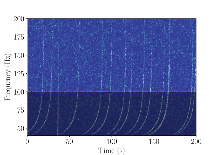
Now that we have shown how the binary neutron star background can be analyzed analogously to the binary black hole background by focusing on frequencies , we provide additional details for the binary neutron star analysis. We work with chunks of strain data. There are two reasons for this choice: it ensures data can be analyzed efficiently and reduces the probability of obtaining an incomplete signal within each data segment. For each segment , we calculate the likelihood function conditional to the signal and noise hypothesis, and ,
| (4) |
| (5) |
Here, we denote the gravitational waveform in the frequency domain as . In the results presented in this paper, we generate with the IMRPhenomD_NRTidal waveform approximant Husa et al. 2016; Khan et al. 2016; Dietrich et al. 2017, which simulates the merger of a binary neutron star including tidal effects. We also calculate the usual inner product starting at the cutoff frequency Hz,
| (6) |
where is the noise power spectral density of the detector. All calculations are performed within the Bayesian inference library Bilby Ashton et al. 2018 using the nested sampling algorithm Dynesty Speagle et al.. Finally, the posterior probability distribution on the duty cycle is given by Eq. 7 if we assume a uniform prior distribution on ,
| (7) |
II.1 Detection Statistic
To detect the gravitational-wave background, we calculate the Bayes Factor (BF) which is the ratio between the hypothesis that assumes that the data contains gravitational-wave signals and the null hypothesis (there is no gravitational-wave background),
| (8) |
The signal evidence hypothesis, , is obtained by marginalizing over in Eq. 2,
| (9) |
and the noise evidence hypothesis is simply
| (10) |
The detection threshold we use is adopted from the convention suggested in Jeffreys 1961, where we claim that the binary neutron star gravitational-wave background is detected if .
III Time-to-detection
To obtain an estimate of the observation time before we obtain a detection, we simulate eight hours of data containing signal and noise segments. The prior distributions used in our search are shown in Tab. 1. We set the spins to zero in all injections and we also marginalize over time of coalescence, phase of coalescence and luminosity distance. Then, for each segment, we calculate the values of and 11 1 We find that the values of are sometimes slightly underestimated using the nested sampling algorithm Dynesty Speagle et al.. However, we show that the posterior distribution of the duty cycle is still unbiased (see Fig. 2) . In this study, we recover the signal and noise evidence using the same prior as the injected signals distributions. If the priors used for parameter estimation do not match the astrophysical distributions, we find the the duty cycle posterior is unbiased as long as the mass priors overlap. If the mass priors do not overlap, then the search only detects the signals with masses common to both priors.
| Parameter | Unit | Prior | Minimum | Maximum |
|---|---|---|---|---|
| uniform | 1.2 | 1.3 | ||
| - | uniform | 0.5 | 1 | |
| RA | rad. | uniform | 0 | |
| DEC | rad. | cos | ||
| - | uniform | -1 | 1 | |
| rad. | uniform | 0 | ||
| rad. | uniform | 0 | ||
| Gpc | comoving | 0.2 | 1 |
The choice of the maximum luminosity distance of our search is . Beyond this distance, the search begins to suffer from bias due to underestimate of the signal evidence22 2 By employing a cut on the maximum distance , we introduce a small bias from the signal coming from . This bias can be estimated and removed in post-processing using mock data.. Work is ongoing to mitigate this bias, which would enable us to extend the maximum distance. Up to this distance, we expect on average one binary neutron star merger every two hours, which translates to a duty cycle of . Due to computational limitations, we cannot simulate the number of segments that will lead to such a duty cycle, however, we can extrapolate our results using a Gaussian mixture model to fit the distributions of the signal and noise evidence Pedregosa et al. 2011; Li 2009. Our analysis assumes a three detector network – LIGO Hanford, LIGO Livingston and Virgo – operating at design sensitivity.
Assuming a merger rate of one signal every two hours, we simulate 30 realizations of the gravitational-wave background and we find that we need to observe for days (one-sigma confidence) to reach the detection threshold of . The number of days needed to make a detection would likely decrease if the maximum luminosity distance of the search can be increased.
The evolution of the posterior probability distribution of as a function of time is presented in Fig. 2. The result shown in the top panel of Fig. 2 shows how the duty cycle posterior distribution evolves over time. After 97 days of observation the posterior recovers the duty-cycle, at this point log BF = 8. After 150 days the .
The strength of the stochastic background signal depends in part on the (somewhat arbitrary) definition of resolvability, which we set to . We vary to see how the search sensitivity scales with this definition. By lowering to eight, we find that the duty-cycle posterior distribution remains unbiased. However, the time to detection increases from to . For , we find that the background can be detected after . Thus, roughly half of the stochastic signal is obtained from signals with signal-to-noise-ratio between eight and ten. It is possible that we might be able to get more stochastic signal from low signal-to-noise ratio events by improving the sampling algorithm and extending the maximum luminosity distance of the search. This is something we hope to explore in future work.
We compare the sensitivity of our Bayesian method to cross-correlation, which is typically cast within the frequentist framework. It is not entirely straightforward to compare frequentist and Bayesian detection statistics. However, if we assume the conventional detection thresholds of for the Bayesian algorithm and the “five-sigma” threshold for the cross-correlation analysis, then we find that the Bayesian analysis here will result in a detection approximately ten times faster than the cross-correlation statistic.
For simplicity, in this study we do not account for “glitches”: noise transients caused by the instrument or the environment, usually from unknown origin Pankow et al. 2018. However, in Ref. Smith and Thrane 2018 it was shown that glitches can be included in our search’s framework.
IV Constraining the equation of state
Neutron stars are ideal objects to study matter at supernuclear densities. The behaviour of neutron stars is governed by the equation of state (EOS), which describes a relationship between state variables such as density and pressure (see, e.g., Baldo and Burgio 2016; Hebeler et al. 2013; Haensel et al. 2007 for a review). This relation, together with the general relativity equations for hydrostatic equilibrium, give a relationship between mass and radius of a neutron star. Such a relation can be constrained by gravitational waves if we can measure the dimensionless tidal deformability , which determines how much a neutron star deforms in the presence of another massive object. The dimensionless tidal deformability depends on the radius of a neutron star and the second love number , , where is the compactness Flanagan and Hinderer 2008. Both of these quantities depend on the equation of state and it is for this reason that in principle, constraining the value of leads to a constraint on the equation of state.
Lackey and Wade Lackey and Wade 2015 showed that the tidal deformability can be measured to 10 - 50 % (depending on the equation of state and mass distribution) with 40 binary neutron star detections, although the majority of information comes from the loudest five events. To date, constraints from LIGO place at the level (for a 1.4 neutron star) Abbott et al. 2018b.
With our method, we can constrain the equation of state using solely sub-threshold signals. The main idea is that the signal and noise evidences, and respectively, will be different depending on which equation of state we use as a prior. We can therefore extract information about the equation of state by calculating the Bayes factor between any two different models,
| (11) |
where are the Bayesian evidences from Eq. 9 with a fixed equation of state prior,
| (12) |
Using simulated data, we compare two equations of state covering different values of stiffness: SLY () Douchin and Haensel 2001 and H4 () Read et al. 2009. Here, the sub-index stands for the dimentionless tidal deformability of a neutron star of 1.4 solar masses. We inject simulated data with the SLY equation of state and then recover the evidences and . We calculate Eq. 7, assuming different observation times starting from one day to 150 days. We then simulate 30 realization of the background and we find that in order to be able to distinguish between SLY and H4, we need to analyze days of data (one-sigma confidence), as shown in Fig. 3. If we analyze all of the events in our dataset, not just the sub-threshold ones, then we expect (on average) to distinguish between these two equations of state after 1.6 months of observation.
The measurement of GW170817 already rules out H4 at 90% confidence Abbott et al. 2018b. We will learn more about the equation state from the loud, resolvable events. However, it is remarkable that we can use unresolved binary neutron stars to say anything about the neutron star equation of state. The constraints obtained by sub-threshold signals can be compared to the results obtained using resolved binary neutron stars as a sanity check, or the two results can be combined to obtain improved sensitivity.
V Conclusions
We derive a method which would detect the binary neutron star gravitational-wave background after days of observation using design-sensitivity aLIGO and Virgo data assuming a merger rate of one signal every two hours, which is consistent with a realistic binary neutron star merger rate Abbott et al. 2017. Future studies will focus on optimizing our search to be able to recover the signal evidence at distances larger than 1 Gpc. More sophisticated analyses will additionally include hierarchical Bayesian inference, which can provide new and complementary insights to the distribution of masses and tidal deformabilities of neutron stars Talbot and Thrane 2018.
Acknowledgments
This work is supported through Australian Research Council (ARC) Centre of Excellence CE170100004. ET is supported through ARC Future Fellowship FT150100281. PDL is supported through ARC Future Fellowship FT160100112 and ARC Discovery Project DP180103155. FHV is supported through the Monash Graduate Scholarship (MGS). The results presented in this manuscript were calculated using the supercomputer clusters at California Institute of Technology and Swinburne University of Technology (OzSTAR). The authors are grateful for computational resources provided by the LIGO Laboratory and supported by National Science Foundation Grants PHY-0757058 and PHY-0823459.
References
- Abbott et al. (2018a) B. P. Abbott et al. (LIGO Scientific Collaboration and Virgo Collaboration), Phys. Rev. Lett. 120, 091101 (2018a).
- Abbott et al. (2017) B. P. Abbott et al. (LIGO Scientific Collaboration and Virgo Collaboration), Phys. Rev. Lett. 119, 161101 (2017).
- Abbott et al. (2015) B. P. Abbott et al. (The LIGO Scientific Collaboration and the Virgo Collaboration), Classical and Quantum Gravity 32, 074001 (2015).
- Aasi et al. (2015) J. Aasi et al., Classical and Quantum Gravity 32, 115012 (2015).
- Acernese et al. (2014) F. Acernese et al., Classical and Quantum Gravity 32, 024001 (2014).
- Allen and Romano (1999) B. Allen and J. D. Romano, Phys. Rev. D 59, 102001 (1999).
- Allen (1996) B. Allen, Relativistic gravitation and gravitational radiation. (1996) pp. 373–417, arXiv:gr-qc/9604033 [gr-qc] .
- Smith and Thrane (2018) R. Smith and E. Thrane, Phys. Rev. X8, 021019 (2018), 1712.00688 .
- Rosado (2011) P. A. Rosado, Phys. Rev. D 84, 084004 (2011).
- Thrane (2013) E. Thrane, Phys. Rev. D 87, 043009 (2013).
- Smith et al. (2016) R. Smith, S. E. Field, K. Blackburn, C.-J. Haster, M. Pürrer, V. Raymond, and P. Schmidt, Phys. Rev. D 94, 044031 (2016).
- Harry and Hinderer (2018) I. Harry and T. Hinderer, Class. Quant. Grav. 35, 145010 (2018).
- Callister et al. (2016) T. Callister, L. Sammut, S. Qiu, I. Mandel, and E. Thrane, Phys. Rev. X 6, 031018 (2016).
- GREEN (1995) P. J. GREEN, Biometrika 82, 711 (1995), http://oup.prod.sis.lan/biomet/article-pdf/82/4/711/699533/82-4-711.pdf .
- Husa et al. (2016) S. Husa, S. Khan, M. Hannam, M. Pürrer, F. Ohme, X. J. Forteza, and A. Bohé, Phys. Rev. D 93, 044006 (2016).
- Khan et al. (2016) S. Khan, S. Husa, M. Hannam, F. Ohme, M. Pürrer, X. J. Forteza, and A. Bohé, Phys. Rev. D 93, 044007 (2016).
- Dietrich et al. (2017) T. Dietrich, S. Bernuzzi, and W. Tichy, Phys. Rev. D 96, 121501 (2017).
- Ashton et al. (2018) G. Ashton et al., (2018), arXiv:1811.02042 [astro-ph.IM] .
- (19) J. Speagle et al., “Dynesty,” https://github.com/joshspeagle/dynesty/.
- Jeffreys (1961) H. Jeffreys, Theory of Probability, 3rd ed. (Oxford, Oxford, England, 1961).
- Pedregosa et al. (2011) F. Pedregosa, G. Varoquaux, A. Gramfort, V. Michel, B. Thirion, O. Grisel, M. Blondel, P. Prettenhofer, R. Weiss, V. Dubourg, J. Vanderplas, A. Passos, D. Cournapeau, M. Brucher, M. Perrot, and E. Duchesnay, Journal of Machine Learning Research 12, 2825 (2011).
- Li (2009) S. Z. Li, Encyclopedia of Biometrics, 1st ed. (Springer Publishing Company, Incorporated, 2009).
- Pankow et al. (2018) C. Pankow, K. Chatziioannou, E. A. Chase, T. B. Littenberg, M. Evans, J. McIver, N. J. Cornish, C.-J. Haster, J. Kanner, V. Raymond, S. Vitale, and A. Zimmerman, Phys. Rev. D 98, 084016 (2018).
- Baldo and Burgio (2016) M. Baldo and G. Burgio, Progress in Particle and Nuclear Physics 91, 203 (2016).
- Hebeler et al. (2013) K. Hebeler, J. M. Lattimer, C. J. Pethick, and A. Schwenk, The Astrophysical Journal 773, 11 (2013).
- Haensel et al. (2007) P. Haensel, A. Y. Potekhin, and D. G. Yakovlev, Astrophys. Space Sci. Libr. 326, pp.1 (2007).
- Flanagan and Hinderer (2008) E. E. Flanagan and T. Hinderer, Phys. Rev. D 77, 021502 (2008).
- Lackey and Wade (2015) B. D. Lackey and L. Wade, Phys. Rev. D 91, 043002 (2015).
- Abbott et al. (2018b) B. P. Abbott et al. (The LIGO Scientific Collaboration and the Virgo Collaboration), Phys. Rev. Lett. 121, 161101 (2018b).
- Douchin and Haensel (2001) F. Douchin and P. Haensel, Astron. Astrophys. 380, 151 (2001), astro-ph/0111092 .
- Read et al. (2009) J. S. Read, B. D. Lackey, B. J. Owen, and J. L. Friedman, Phys. Rev. D 79, 124032 (2009).
- Talbot and Thrane (2018) C. Talbot and E. Thrane, The Astrophysical Journal 856, 173 (2018).