跳到论文正文
W Papers独立论文阅读器 arXiv:1903.05655 论文正文 计算阅读时间 · 0%
引用这篇论文根据当前论文元数据生成,正式投稿前建议核对。


License: arXiv.org perpetual non-exclusive license
arXiv:1903.05655v1 [math.GT] 13 Mar 2019

Strands algebras and Ozsváth–Szabó’s Kauffman-states functorThanks: AM was supported by an NSF MSPRF fellowship, grant number DMS-1502686.Thanks: MW was supported by the NSF grant DMS-1563615.

Andrew Manion Address: Department of Mathematics, USC, 3620 S. Vermont Ave., Los Angeles, CA 90089 Email address: amanion@usc.edu , Marco Marengon Address: Department of Mathematics, UCLA, 520 Portola Plaza, Los Angeles, CA 90095 Email address: marengon@math.ucla.edu and Michael Willis Address: Department of Mathematics, UCLA, 520 Portola Plaza, Los Angeles, CA 90095 Email address: mike.willis@math.ucla.edu
Abstract.

We define new differential graded algebras 𝒜⁡(n,k,𝒮)\mathcal{A}(n,k,\mathcal{S}) in the framework of Lipshitz–Ozsváth–Thurston’s and Zarev’s strands algebras from bordered Floer homology. The algebras 𝒜⁡(n,k,𝒮)\mathcal{A}(n,k,\mathcal{S}) are meant to be strands models for Ozsváth–Szabó’s algebras ℬ⁡(n,k,𝒮)\mathcal{B}(n,k,\mathcal{S}); indeed, we exhibit a quasi-isomorphism from ℬ⁡(n,k,𝒮)\mathcal{B}(n,k,\mathcal{S}) to 𝒜⁡(n,k,𝒮)\mathcal{A}(n,k,\mathcal{S}). We also show how Ozsváth–Szabó’s gradings on ℬ⁡(n,k,𝒮)\mathcal{B}(n,k,\mathcal{S}) arise naturally from the general framework of group-valued gradings on strands algebras.

1. Introduction

Heegaard Floer homology is a package of invariants for 3-manifolds and 4-manifolds introduced by Ozsváth and Szabó [OSz04c, OSz04b] that has proven to be particularly powerful in the last two decades. A variation [OSz04a, Ras03] of their construction, called knot Floer homology and abbreviated H​F​KHFK, assigns a graded abelian group to a knot or link, and the Euler characteristic of this group recovers the Alexander polynomial. Knot Floer homology has many applications in knot theory; for example, it exactly characterizes elusive knot information like Seifert genus and fiberedness, for which the knot polynomials provide only incomplete bounds, and it leads to the definition of many interesting knot concordance invariants.

In the past ten years, there has been considerable interest in assigning Heegaard Floer invariants to surfaces and 33-dimensional cobordisms between them. Lipshitz–Ozsváth–Thurston’s bordered Floer homology [LOT18] initiated this project; Zarev [Zar09] introduced a generalization known as bordered sutured Floer homology. If one views Heegaard Floer homology from the perspective of topological quantum field theories (TQFTs), then bordered Floer homology begins the investigation of Heegaard Floer homology as an “extended” TQFT. Extensions of TQFTs have been of particular interest since Lurie’s proof [Lur09] of the Baez–Dolan cobordism hypothesis classifying fully extended TQFTs.

Bordered sutured Floer homology assigns an invariant to a surface FF by first choosing a combinatorial representation of FF, called an “arc diagram” by Zarev. Arc diagrams are a special case of what are known as “chord diagrams” in e.g. [AFM+17] (see Definition 3.1). Chord diagrams may have linear and/or circular “backbones” (see Figure 1); arc diagrams are the same as chord diagrams with no circular backbones. To an arc diagram 𝒵\mathcal{Z} representing a surface F⁡(𝒵)F(\mathcal{Z}), bordered sutured Floer homology associates a differential graded (dg) algebra 𝒜⁡(𝒵)\mathcal{A}(\mathcal{Z}), called the bordered strands algebra of 𝒵\mathcal{Z} because it can be visualized by pictures of strands intersecting in [0,1]×𝒵[0,1]\times\mathcal{Z}. Auroux [Aur10] has shown that 𝒜⁡(𝒵)\mathcal{A}(\mathcal{Z}) is closely related to Fukaya categories of symmetric powers of F⁡(𝒵)F(\mathcal{Z}), in line with the original definition of Heegaard Floer homology.

More recently, Ozsváth–Szabó [OSz18, OSz17, OSza, OSzc] have used the ideas of bordered Floer homology to define a new algorithmic method for computing H​F​KHFK by decomposing a knot into tangles. Their theory has striking computational properties [OSzb], categorifies aspects of the representation theory of 𝒰q​(𝔤​𝔩​(1|1))\mathcal{U}_{q}(\mathfrak{gl}(1|1)) [Man19], and has surprising connections with other such categorifications [Man17]. We will refer to their theory as the Kauffman-states functor, since Kauffman states for a knot or tangle projection (equivalently, spanning trees of the Tait graph) play a prominent role.

Refer to caption
Figure 1. The Heegaard diagram motivating the Kauffman-states functor, and the chord diagram implied by it. Such a chord diagram has 22 linear backbones and 33 circular backbones (all drawn in black).

To a tangle diagram, the Kauffman-states functor assigns a bimodule whose definition is motivated by holomorphic curve counting as in bordered Floer homology. However, the dg algebras ℬ⁡(n,𝒮)\mathcal{B}(n,\mathcal{S}) over which the bimodule is defined are not among Zarev’s bordered strands algebras. Indeed, for a single crossing, Ozsváth–Szabó count curves in a particular Heegaard diagram from which a chord diagram 𝒵⁡(n)\mathcal{Z}(n) can be inferred (see Figure 1), but some of the backbones of 𝒵⁡(n)\mathcal{Z}(n) are circular rather than linear, so 𝒵⁡(n)\mathcal{Z}(n) is not an arc diagram and Zarev’s construction does not apply.

We begin by defining a reasonable candidate 𝒜⁡(n,𝒮)\mathcal{A}(n,\mathcal{S}) for the bordered strands algebra of the chord diagram 𝒵⁡(n)\mathcal{Z}(n) in question, with a diagrammatic interpretation in terms of intersecting strands as usual (the data 𝒮\mathcal{S} encodes orientations on tangle endpoints and will be described below in Section 2). The algebra 𝒜⁡(n,𝒮)\mathcal{A}(n,\mathcal{S}) is larger than ℬ⁡(n,𝒮)\mathcal{B}(n,\mathcal{S}), with a more elaborate differential. See e.g. Figure 6 for an illustration. The dg algebras 𝒜⁡(n,𝒮)\mathcal{A}(n,\mathcal{S}) and ℬ⁡(n,𝒮)\mathcal{B}(n,\mathcal{S}) are both direct sums of dg algebras 𝒜⁡(n,k,𝒮)\mathcal{A}(n,k,\mathcal{S}) and ℬ⁡(n,k,𝒮)\mathcal{B}(n,k,\mathcal{S}) for 0≤k≤n0\leq k\leq n. Like ℬ⁡(n,k,𝒮)\mathcal{B}(n,k,\mathcal{S}), the strands algebra 𝒜⁡(n,k,𝒮)\mathcal{A}(n,k,\mathcal{S}) comes with a Maslov grading and various Alexander multi-gradings.

The bordered strands algebra 𝒜⁡(n,k,𝒮)\mathcal{A}(n,k,\mathcal{S}) and Ozsváth–Szabó’s algebra ℬ⁡(n,k,𝒮)\mathcal{B}(n,k,\mathcal{S}) are in fact closely related to each other. Using the generators-and-relations description of ℬ⁡(n,k,𝒮)\mathcal{B}(n,k,\mathcal{S}) from [MMW19], we define a dg algebra homomorphism Φ:ℬ⁡(n,k,𝒮)→𝒜⁡(n,k,𝒮)\Phi:\mathcal{B}(n,k,\mathcal{S})\to\mathcal{A}(n,k,\mathcal{S}) and prove the following result.

Theorem 1.1.

The map Φ:ℬ⁡(n,k,𝒮)→𝒜⁡(n,k,𝒮)\Phi:\mathcal{B}(n,k,\mathcal{S})\to\mathcal{A}(n,k,\mathcal{S}) is a quasi-isomorphism.

Since we computed the homology of ℬ⁡(n,k,𝒮)\mathcal{B}(n,k,\mathcal{S}) in [MMW19], we deduce the homology of 𝒜⁡(n,k,𝒮)\mathcal{A}(n,k,\mathcal{S}) from Theorem 1.1.

Corollary 1.2.

Applying Φ\Phi to the basis for H∗​(ℬ​(n,k,𝒮))H_{*}(\mathcal{B}(n,k,\mathcal{S})) given in Theorem 2.20 yields a basis for H∗​(𝒜​(n,k,𝒮))H_{*}(\mathcal{A}(n,k,\mathcal{S})).

We can also transfer the formality properties for ℬ⁡(n,k,𝒮)\mathcal{B}(n,k,\mathcal{S}) proved in [MMW19] to the quasi-isomorphic algebras 𝒜⁡(n,k,𝒮)\mathcal{A}(n,k,\mathcal{S}).

Corollary 1.3.

The dg algebra 𝒜⁡(n,k,𝒮)\mathcal{A}(n,k,\mathcal{S}) is formal if and only if 𝒮=∅\mathcal{S}=\varnothing or k∈{0,n,n+1}k\in\{0,n,n+1\}.

We describe the gradings on 𝒜⁡(n,k,𝒮)\mathcal{A}(n,k,\mathcal{S}) combinatorially in Definition 6.1; their definition depends on 𝒮\mathcal{S}. However, bordered strands algebras 𝒜⁡(𝒵)\mathcal{A}(\mathcal{Z}) typically have gradings by nonabelian groups G′​(𝒵)G^{\prime}(\mathcal{Z}) and G⁡(𝒵)G(\mathcal{Z}) which do not see the dependence on 𝒮\mathcal{S}. We define these gradings in our setting too (both groups end up being abelian) and show how they are related to the combinatorial gradings.

Theorem 1.4.

Given 𝒮\mathcal{S}, we have an isomorphism

Θ𝒮:G′​(𝒵⁡(n))→≅ℤ⊕ℤ2​n\Theta_{\mathcal{S}}:G^{\prime}(\mathcal{Z}(n))\xrightarrow{\cong}\mathbb{Z}\oplus\mathbb{Z}^{2n}

such that for a homogeneous element aa of 𝒜⁡(n,k,𝒮)\mathcal{A}(n,k,\mathcal{S}), the first component of Θ𝒮​(deg′⁡(a))\Theta_{\mathcal{S}}(\deg^{\prime}(a)) is the Maslov degree of aa and the rest of the components form the unrefined Alexander multi-degree of aa. Similarly, we have an isomorphism

Θ𝒮:G⁡(𝒵⁡(n))→≅ℤ⊕(12​ℤ)n\Theta_{\mathcal{S}}:G(\mathcal{Z}(n))\xrightarrow{\cong}\mathbb{Z}\oplus\left(\textstyle{\frac{1}{2}}\mathbb{Z}\right)^{n}

whose first component recovers the Maslov grading and whose second component recovers the refined Alexander multi-grading.

Theorem 1.4 helps to explain the appearance of the data 𝒮\mathcal{S} in the algebras 𝒜⁡(n,k,𝒮)\mathcal{A}(n,k,\mathcal{S}) and ℬ⁡(n,k,𝒮)\mathcal{B}(n,k,\mathcal{S}), since the orientation data for tangle endpoints is not visible from the chord diagram 𝒵⁡(n)\mathcal{Z}(n). While the gradings by G′​(𝒵​(n))G^{\prime}(\mathcal{Z}(n)) and G⁡(𝒵⁡(n))G(\mathcal{Z}(n)) are independent of this orientation data, their interpretation as standard Maslov and Alexander gradings is noncanonical and its choice forces a choice of 𝒮\mathcal{S}.

We note that this noncanonicity stems from the condition “j≡ε⁡(α)j\equiv\varepsilon(\alpha) mod 11” in Lipshitz–Ozsváth–Thurston’s definition of their nonabelian gradings (see [LOT18, Definition 3.33]). Thus, we have a new motivation for this somewhat mysterious-seeming condition, since in the end we do want 𝒜⁡(n,k,𝒮)\mathcal{A}(n,k,\mathcal{S}) and ℬ⁡(n,k,𝒮)\mathcal{B}(n,k,\mathcal{S}) to depend on orientations. Note, however, that 𝒜⁡(n,k,𝒮)\mathcal{A}(n,k,\mathcal{S}) and ℬ⁡(n,k,𝒮)\mathcal{B}(n,k,\mathcal{S}) depend on 𝒮\mathcal{S} for more than just their gradings; 𝒮\mathcal{S} also determines whether certain additional generators are allowed in the algebras.

Along with ℬ⁡(n,k,𝒮)\mathcal{B}(n,k,\mathcal{S}), it is natural to consider certain idempotent-truncated algebras ℬr​(n,k,𝒮)\mathcal{B}_{r}(n,k,\mathcal{S}), ℬl​(n,k,𝒮)\mathcal{B}_{l}(n,k,\mathcal{S}), and ℬ′​(n,k,𝒮)\mathcal{B}^{\prime}(n,k,\mathcal{S}). Each has an associated chord diagram 𝒵r​(n)\mathcal{Z}_{r}(n), 𝒵l​(n)\mathcal{Z}_{l}(n), or 𝒵′​(n)\mathcal{Z}^{\prime}(n), and we define the corresponding strands algebras 𝒜r​(n,k,𝒮)\mathcal{A}_{r}(n,k,\mathcal{S}), 𝒜l​(n,k,𝒮)\mathcal{A}_{l}(n,k,\mathcal{S}), and 𝒜′​(n,k,𝒮)\mathcal{A}^{\prime}(n,k,\mathcal{S}) (they are idempotent truncations of 𝒜⁡(n,k,𝒮)\mathcal{A}(n,k,\mathcal{S})). We prove that Φ\Phi gives a quasi-isomorphism between the truncated algebras as well, deducing results about homology and formality for the truncated algebras from the analogous results in [MMW19].

Finally, we define symmetries on the strands algebras 𝒜⁡(n,k,𝒮)\mathcal{A}(n,k,\mathcal{S}) analogous to Ozsváth–Szabó’s symmetries ℛ\mathcal{R} and oo on the algebras ℬ⁡(n,k,𝒮)\mathcal{B}(n,k,\mathcal{S}), and we show that Φ\Phi preserves these symmetries. The symmetries on 𝒜⁡(n,k,𝒮)\mathcal{A}(n,k,\mathcal{S}) have an appealing visual interpretation as symmetries of the surface [0,1]×𝒵⁡(n)[0,1]\times\mathcal{Z}(n) on which the strands pictures are drawn.

Context and motivation

This paper is a sequel to [MMW19], which lays much of the necessary groundwork for our main results here. A third paper [MMW] in the series is planned, in which we define bimodules over 𝒜⁡(n,k,𝒮)\mathcal{A}(n,k,\mathcal{S}) for crossings and prove that they are compatible with Ozsváth–Szabó’s bimodules in an appropriate sense.

We view our constructions as evidence for the existence of a generalized theory of bordered sutured Floer homology, allowing chord diagrams with circular backbones and correspondingly generalized Heegaard diagrams. Defining Heegaard Floer homology analytically in this level of generality has not been attempted, and appears to be quite difficult. However, various recent constructions should be special cases of such a generalized theory, including Lipshitz–Ozsváth–Thurston’s work in progress on a bordered H​F−HF^{-} theory for 33-manifolds with torus boundary [LOT] as well as Zibrowius’ constructions in [Zib19]. Our work should enable Ozsváth–Szabó’s Kauffman-states functor to be directly compared with such a generalized theory once it exists, unifying the Kauffman-states functor with the rest of bordered Floer homology.

In [MR], Raphaël Rouquier and the first named author will define generalized strands algebras 𝒜⁡(𝒵)\mathcal{A}(\mathcal{Z}), including 𝒜⁡(n,k,𝒮)\mathcal{A}(n,k,\mathcal{S}) as a special case. These algebras are candidates for the algebras appearing in a generalized bordered sutured theory, possibly after deformation as in [LOT]. The constructions of [MR] will also give 𝒜⁡(𝒵)\mathcal{A}(\mathcal{Z}) the structure of a 22-representation of Khovanov’s categorified 𝒰q+​(𝔤​𝔩​(1|1))\mathcal{U}_{q}^{+}(\mathfrak{gl}(1|1)). Thus, together with [MR], this paper fills in (the positive half of) a missing piece from the discussion of [Man19]. While [Man19] shows that the bimodules from the Kauffman-states functor categorify 𝒰q​(𝔤​𝔩​(1|1))\mathcal{U}_{q}(\mathfrak{gl}(1|1))-intertwining maps between representations, no candidate was offered for the categorification of the 𝒰q​(𝔤​𝔩​(1|1))\mathcal{U}_{q}(\mathfrak{gl}(1|1)) actions on the representations. This paper allows us to replace Ozsváth–Szabó’s algebra ℬ⁡(n,k,𝒮)\mathcal{B}(n,k,\mathcal{S}) (when desired) with a strands algebra 𝒜⁡(n,k,𝒮)\mathcal{A}(n,k,\mathcal{S}) on which a categorified quantum-group action is given in [MR]. Alternatively, one could directly define a 22-action on ℬ⁡(n,k,𝒮)\mathcal{B}(n,k,\mathcal{S}), and show that it is compatible with the 22-action on 𝒜⁡(n,k,𝒮)\mathcal{A}(n,k,\mathcal{S}) via Φ\Phi; the first named author plans to do this once the general framework of [MR] is available.

This paper, along with [MMW19], only discusses the algebras coming from Ozsváth–Szabó’s first paper [OSz18] on the Kauffman-states functor. A variant of these algebras was introduced in [OSz17], and further variants will be defined in [OSza, OSzc]. It would be very interesting to find analogues of the results of this paper for any of these algebras, especially the “Pong algebra” from [OSzc]. As with Lipshitz–Ozsváth–Thurston’s constructions in [LOT], the Pong algebra may give further insight into the algebraic structure required for a generalized bordered sutured theory as mentioned above.

For the reasons discussed in [MMW19], we will follow the standard conventions in bordered Floer homology and work over 𝔽2\mathbb{F}_{2}. While the bordered strands algebras have not been defined over ℤ\mathbb{Z} in general, to the authors’ knowledge, it is plausible that the constructions in this paper could be done over ℤ\mathbb{Z}. However, it is likely that an analytic generalization of bordered sutured Floer homology would be considerably more difficult over ℤ\mathbb{Z} than over 𝔽2\mathbb{F}_{2}.

Organization

We start with a brief review of some essential definitions and results from [MMW19] in Section 2. For motivation, we discuss chord diagrams and sutured surfaces in Section 3, giving generalized versions of Zarev’s definitions.

In Section 4, we define the strands algebras 𝒜⁡(n,k,𝒮)\mathcal{A}(n,k,\mathcal{S}) and give illustrations. Section 5 proves some properties that will be useful both here and in [MMW]; in particular, we give an explicit calculus for products and differentials of certain basis elements of 𝒜⁡(n,k,𝒮)\mathcal{A}(n,k,\mathcal{S}). In Section 6 we discuss gradings and prove Theorem 1.4; in Section 7, we define symmetries on 𝒜⁡(n,k,𝒮)\mathcal{A}(n,k,\mathcal{S}).

In Section 8 we compute the homology of 𝒜⁡(n,k,∅)\mathcal{A}(n,k,\varnothing). In Section 9 we define the map Φ\Phi from ℬ⁡(n,k,𝒮)\mathcal{B}(n,k,\mathcal{S}) to 𝒜⁡(n,k,𝒮)\mathcal{A}(n,k,\mathcal{S}) and prove Theorem 1.1 by induction on |𝒮||\mathcal{S}|; the base case of the induction (|𝒮|=0|\mathcal{S}|=0) follows from the computation of H∗​(𝒜⁡(n,k,∅))H_{*}(\mathcal{A}(n,k,\varnothing)) in Section 8. Finally, in Section 9.3 we show that Φ\Phi preserves the algebra symmetries.

Acknowledgments

The authors would like to thank Francis Bonahon, Ko Honda, Aaron Lauda, Robert Lipshitz, Ciprian Manolescu, Peter Ozsváth, Raphaël Rouquier, and Zoltán Szabó for many useful conversations. The first named author would especially like to thank Zoltán Szabó for teaching him about the Kauffman-states functor.

2. Background on Ozsváth–Szabó’s algebras

We begin with a brief review of some important terminology and results from [OSz18, MMW19]. As in [MMW19, Appendix A], given a commutative ring 𝕜\Bbbk, we define a 𝕜\Bbbk-algebra to be a ring 𝒜\mathcal{A} equipped with a ring homomorphism 𝕜→𝒜\Bbbk\to\mathcal{A}. Given a quiver Γ\Gamma (i.e. a finite directed graph, allowed to have loops and multi-edges), one has a path algebra Path⁡(Γ)\Path(\Gamma) formally spanned over 𝕜\Bbbk by paths in Γ\Gamma, with multiplication given by concatenation. If VV is the vertex set of Γ\Gamma, one can view Path⁡(Γ)\Path(\Gamma) as an algebra over 𝕀=𝕜V\mathbb{I}=\Bbbk^{V}, the ring of functions from VV into 𝕜\Bbbk. The homomorphism 𝕀→Path⁡(Γ)\mathbb{I}\to\Path(\Gamma) sends the indicator function of a vertex 𝐱\mathbf{x} to the empty path 𝐈𝐱\mathbf{I}_{\mathbf{x}} based at 𝐱\mathbf{x}. The composition 𝕜→𝕀→Path⁡(Γ)\Bbbk\to\mathbb{I}\to\Path(\Gamma) has image in the center of Path⁡(Γ)\Path(\Gamma).

Equivalently, one may work in terms of a 𝕜\Bbbk-linear category 𝕜​Γ\Bbbk\Gamma whose set of objects is VV; see [MMW19, Section 2.1 and Appendix A] for a detailed review of this algebraic framework. Hom-spaces in this category are given by 𝐈𝐱​Path⁡(Γ)​𝐈𝐲\mathbf{I}_{\mathbf{x}}\Path(\Gamma)\mathbf{I}_{\mathbf{y}} for 𝐱,𝐲∈V\mathbf{x},\mathbf{y}\in V, and we have a decomposition

Path⁡(Γ)≅⨁𝐱,𝐲∈V𝐈𝐱​Path⁡(Γ)​𝐈𝐲.\Path(\Gamma)\cong\bigoplus_{\mathbf{x},\mathbf{y}\in V}\mathbf{I}_{\mathbf{x}}\Path(\Gamma)\mathbf{I}_{\mathbf{y}}.

If ℛ\mathcal{R} is a subset of Path⁡(Γ)\Path(\Gamma), we can also consider the quotient of Path⁡(Γ)\Path(\Gamma) by the two-sided ideal generated by ℛ\mathcal{R}. We will call this quotient Quiv⁡(Γ,ℛ)\Quiv(\Gamma,\mathcal{R}); it is still an algebra over 𝕀\mathbb{I}, and we can still view it as a 𝕜\Bbbk-linear category. Gradings and differentials on Path⁡(Γ)\Path(\Gamma) and Quiv⁡(Γ,ℛ)\Quiv(\Gamma,\mathcal{R}) can be specified by defining them on the edges of Γ\Gamma, as long as the relations are homogeneous cycles, so that we can consider dg algebras defined by quiver generators and relations.

Convention 2.1.

In this paper, as in [MMW19], the interval [a,b][a,b] will denote the set of integers ii with a≤i≤ba\leq i\leq b.

Given a subset 𝒮⊂[1,n]\mathcal{S}\subset[1,n], we now recall the definition of Ozsváth–Szabó’s algebra ℬ⁡(n,k,𝒮)\mathcal{B}(n,k,\mathcal{S}) in the language of [MMW19].

Definition 2.2.

For n≥0n\geq 0 and 0≤k≤n0\leq k\leq n, let V⁡(n,k)V(n,k) denote the set of kk-element subsets 𝐱⊂[0,n]\mathbf{x}\subset[0,n]. Elements of V⁡(n,k)V(n,k) will sometimes be called I-states, following [OSz18, Section 3.1]. Taking 𝕜=𝔽2\Bbbk=\mathbb{F}_{2}, let 𝐈⁡(n,k)=𝔽2V⁡(n,k)\mathbf{I}(n,k)=\mathbb{F}_{2}^{V(n,k)}.

Elements of V⁡(n,k)V(n,k) are visualized as in Figure 2. Elements of [0,n][0,n] are thought of as regions between nn parallel horizontal lines, including the two unbounded regions above and below the lines. An I-state 𝐱\mathbf{x} is drawn by placing a dot in each region corresponding to an element of 𝐱\mathbf{x}. Ozsváth and Szabó use a 90∘90^{\circ}-rotated visualization; see Remark 2.11.

Refer to caption
Figure 2. Elements 𝐱\mathbf{x} and 𝐲\mathbf{y} of V⁡(5,3)V(5,3) viewed as dots occupying regions. The left-most figure indicates the numbered labeling of the regions and the lines between them.
Definition 2.3.

The directed graph Γ⁡(n,k,𝒮)\Gamma(n,k,\mathcal{S}) has set of vertices V⁡(n,k)V(n,k). It has the following edges:

  • •

    if 1≤i≤n1\leq i\leq n and 𝐱∩{i−1,i}={i−1}\mathbf{x}\cap\{i-1,i\}=\{i-1\}, then Γ⁡(n,k,𝒮)\Gamma(n,k,\mathcal{S}) has an edge from 𝐱\mathbf{x} to (𝐱∖{i−1})∪{i}(\mathbf{x}\setminus\left\{i-1\right\})\cup\left\{i\right\} labeled RiR_{i};

  • •

    if 1≤i≤n1\leq i\leq n and 𝐱∩{i−1,i}={i}\mathbf{x}\cap\{i-1,i\}=\{i\}, then Γ⁡(n,k,𝒮)\Gamma(n,k,\mathcal{S}) has an edge from 𝐱\mathbf{x} to (𝐱∖{i})∪{i−1}(\mathbf{x}\setminus\left\{i\right\})\cup\left\{i-1\right\} labeled LiL_{i};

  • •

    if 1≤i≤n1\leq i\leq n and 𝐱∈V⁡(n,k)\mathbf{x}\in V(n,k), then Γ⁡(n,k,𝒮)\Gamma(n,k,\mathcal{S}) has an edge from 𝐱\mathbf{x} to itself labeled UiU_{i};

  • •

    if i∈𝒮i\in\mathcal{S} and 𝐱∈V⁡(n,k)\mathbf{x}\in V(n,k), then Γ⁡(n,k,𝒮)\Gamma(n,k,\mathcal{S}) has an edge from 𝐱\mathbf{x} to itself labeled CiC_{i}.

For each path γ\gamma in Γ⁡(n,k,𝒮)\Gamma(n,k,\mathcal{S}), we associate a noncommutative monomial μ⁡(γ)\mu(\gamma) in the letters {Ri,Li,Ui,Ci}\{R_{i},L_{i},U_{i},C_{i}\} by taking the labels of the edges of γ\gamma in order. We extend μ\mu additively to the path algebra of Γ⁡(n,k,𝒮)\Gamma(n,k,\mathcal{S}).

Definition 2.4.

For 𝐱,𝐲∈V⁡(n,k)\mathbf{x},\mathbf{y}\in V(n,k), let ℛ~𝐱,𝐲,𝒮\widetilde{\mathcal{R}}_{\mathbf{x},\mathbf{y},\mathcal{S}} be the set of elements a∈𝐈𝐱​Path⁡(Γ⁡(n,k,𝒮))​𝐈𝐲a\in\mathbf{I}_{\mathbf{x}}\Path(\Gamma(n,k,\mathcal{S}))\mathbf{I}_{\mathbf{y}} such that μ⁡(a)\mu(a) is one of the following:

  • •

    Ri​Uj−Uj​RiR_{i}U_{j}-U_{j}R_{i},  Li​Uj−Uj​LiL_{i}U_{j}-U_{j}L_{i}, or Ui​Uj−Uj​UiU_{i}U_{j}-U_{j}U_{i} (the “UU central relations”)

  • •

    Ri​Li−UiR_{i}L_{i}-U_{i} or Li​Ri−UiL_{i}R_{i}-U_{i} (the “loop relations”)

  • •

    Ri​Rj−Rj​RiR_{i}R_{j}-R_{j}R_{i},  Li​Lj−Lj​LiL_{i}L_{j}-L_{j}L_{i}, or Ri​Lj−Lj​RiR_{i}L_{j}-L_{j}R_{i} for |i−j|>1|i-j|>1 (the “distant commutation relations”)

  • •

    Ri​Ri+1R_{i}R_{i+1} or Li+1​LiL_{i+1}L_{i} (the “two-line pass relations”)

  • •

    UiU_{i} when aa is represented by a loop γ\gamma at a vertex 𝐱\mathbf{x} of V⁡(n,k)V(n,k) such that 𝐱∩{i−1,i}=∅\mathbf{x}\cap\{i-1,i\}=\varnothing (the “UU vanishing relations”)

  • •

    Ci2C_{i}^{2} (the “CC vanishing relations”)

  • •

    Ci​A−A​CiC_{i}A-AC_{i} for any label A∈{Rj,Lj,Uj,Cj}A\in\{R_{j},L_{j},U_{j},C_{j}\} (the “CC central relations”).

Let ℛ~𝒮=⋃𝐱,𝐲∈V⁡(n,k)ℛ~𝐱,𝐲,𝒮\widetilde{\mathcal{R}}_{\mathcal{S}}=\bigcup_{\mathbf{x},\mathbf{y}\in V(n,k)}\widetilde{\mathcal{R}}_{\mathbf{x},\mathbf{y},\mathcal{S}}. Let Quiv⁡(Γ⁡(n,k,𝒮),ℛ~𝒮)\Quiv(\Gamma(n,k,\mathcal{S}),\widetilde{\mathcal{R}}_{\mathcal{S}}) denote the quotient of the path algebra of Γ⁡(n,k,𝒮)\Gamma(n,k,\mathcal{S}) by the two-sided ideal generated by elements of ℛ~𝒮\widetilde{\mathcal{R}}_{\mathcal{S}}. Define a differential on Quiv⁡(Γ⁡(n,k,𝒮),ℛ~𝒮)\Quiv(\Gamma(n,k,\mathcal{S}),\widetilde{\mathcal{R}}_{\mathcal{S}}) by declaring that ∂(Ci)=Ui\partial(C_{i})=U_{i}.

We have a homological grading on Quiv⁡(Γ⁡(n,k,𝒮),ℛ~𝒮)\Quiv(\Gamma(n,k,\mathcal{S}),\widetilde{\mathcal{R}}_{\mathcal{S}}) called the Maslov grading, as well as three related types of intrinsic gradings called Alexander gradings. We recall their definitions now.

Definition 2.5 ([MMW19, Section 3.3]).

The gradings on Quiv⁡(Γ⁡(n,k,𝒮),ℛ~𝒮)\Quiv(\Gamma(n,k,\mathcal{S}),\widetilde{\mathcal{R}}_{\mathcal{S}}) are defined as follows:

  • •

    Let {τ1,…,τn,β1,…,βn}\{\tau_{1},\ldots,\tau_{n},\beta_{1},\ldots,\beta_{n}\} denote the standard basis of ℤ2​n\mathbb{Z}^{2n}. For an edge γ\gamma of Γ⁡(n,k,𝒮)\Gamma(n,k,\mathcal{S}), define the unrefined Alexander multi-degree wun​(γ)∈(ℤ)2​nw^{\un}(\gamma)\in(\mathbb{Z})^{2n} to be

    • *

      wun​(γ)=τiw^{\un}(\gamma)=\tau_{i} if γ\gamma has label RiR_{i}

    • *

      wun​(γ)=βiw^{\un}(\gamma)=\beta_{i} if γ\gamma has label LiL_{i}

    • *

      wun​(γ)=τi+βiw^{\un}(\gamma)=\tau_{i}+\beta_{i} if γ\gamma has label UiU_{i} or CiC_{i}.

    Extend wunw^{\un} additively to any path γ∈Path⁡(Γ⁡(n,k,𝒮))\gamma\in\Path(\Gamma(n,k,\mathcal{S})).

  • •

    Let {e1,…,en}\{e_{1},\ldots,e_{n}\} denote the standard basis of ℤn\mathbb{Z}^{n}. Define the refined Alexander multi-grading on Quiv⁡(Γ⁡(n,k,𝒮),ℛ~𝒮)\Quiv(\Gamma(n,k,\mathcal{S}),\widetilde{\mathcal{R}}_{\mathcal{S}}), a grading by (12​ℤ)n\left(\frac{1}{2}\mathbb{Z}\right)^{n}, by applying the homomorphism ℤ2​n→(12​ℤ)n\mathbb{Z}^{2n}\to\left(\frac{1}{2}\mathbb{Z}\right)^{n} sending τi\tau_{i} and βi\beta_{i} to ei2\frac{e_{i}}{2} to the unrefined Alexander multi-degrees. For a∈Quiv⁡(Γ⁡(n,k,𝒮),ℛ~𝒮)a\in\Quiv(\Gamma(n,k,\mathcal{S}),\widetilde{\mathcal{R}}_{\mathcal{S}}) homogeneous, let w⁡(a)w(a) denote the refined Alexander multi-degree of aa. Explicitly, for an edge γ\gamma of Γ⁡(n,k,𝒮)\Gamma(n,k,\mathcal{S}), we have

    • *

      w⁡(γ)=12​eiw(\gamma)=\frac{1}{2}e_{i} if γ\gamma has label RiR_{i} or LiL_{i}

    • *

      w⁡(γ)=eiw(\gamma)=e_{i} if γ\gamma has label UiU_{i} or CiC_{i}.

    Let wi​(a)w_{i}(a) denote the coefficient of w⁡(a)w(a) on the basis element eie_{i}.

  • •

    Define the single Alexander grading on Quiv⁡(Γ⁡(n,k,𝒮),ℛ~𝒮)\Quiv(\Gamma(n,k,\mathcal{S}),\widetilde{\mathcal{R}}_{\mathcal{S}}), a grading by 12​ℤ\frac{1}{2}\mathbb{Z}, by applying the homomorphism (12​ℤ)n→12​ℤ\left(\frac{1}{2}\mathbb{Z}\right)^{n}\to\frac{1}{2}\mathbb{Z} sending

    ei↦{1 if ​i∉𝒮−1 if ​i∈𝒮e_{i}\mapsto\begin{cases}1&\textrm{ if }i\notin\mathcal{S}\\ -1&\textrm{ if }i\in\mathcal{S}\end{cases}

    to the refined Alexander multi-degrees. Let Alex⁡(a)\Alex(a) denote the single Alexander degree of aa. We have

    Alex⁡(a)=∑i∉𝒮wi​(a)−∑i∈𝒮wi​(a).\Alex(a)=\sum_{i\notin\mathcal{S}}w_{i}(a)-\sum_{i\in\mathcal{S}}w_{i}(a).

    Explicitly, for a single edge γ\gamma, we have

    • *

      Alex⁡(γ)=1/2\Alex(\gamma)=1/2 if γ\gamma has label RiR_{i} or LiL_{i} and i∉𝒮i\notin\mathcal{S}

    • *

      Alex(γ)=−1/2\Alex(\gamma)=-1/2 if γ\gamma has label RiR_{i} or LiL_{i} and i∈𝒮i\in\mathcal{S}

    • *

      Alex⁡(γ)=1\Alex(\gamma)=1 if γ\gamma has label UiU_{i} and i∉𝒮i\notin\mathcal{S}

    • *

      Alex⁡(γ)=−1\Alex(\gamma)=-1 if γ\gamma has label UiU_{i} or CiC_{i} and i∈𝒮i\in\mathcal{S}.

  • •

    Define the Maslov grading on Quiv⁡(Γ⁡(n,k,𝒮),ℛ~𝒮)\Quiv(\Gamma(n,k,\mathcal{S}),\widetilde{\mathcal{R}}_{\mathcal{S}}), a grading by ℤ\mathbb{Z}, by declaring

    𝔪⁡(γ)=#C​(γ)−2​∑i∈𝒮wi​(γ)\mathfrak{m}(\gamma)=\#_{C}(\gamma)-2\sum_{i\in\mathcal{S}}w_{i}(\gamma)

    for a path γ\gamma in Γ⁡(n,k,𝒮)\Gamma(n,k,\mathcal{S}), where #C​(γ)\#_{C}(\gamma) is the number of edges in γ\gamma labeled CiC_{i} for some ii. Explicitly, for a single edge γ\gamma, we have

    • *

      𝔪⁡(γ)=0\mathfrak{m}(\gamma)=0 if γ\gamma has label RiR_{i}, LiL_{i}, or UiU_{i} and i∉𝒮i\notin\mathcal{S}

    • *

      𝔪⁡(γ)=−1\mathfrak{m}(\gamma)=-1 if γ\gamma has label RiR_{i}, LiL_{i}, or CiC_{i} and i∈𝒮i\in\mathcal{S}

    • *

      𝔪⁡(γ)=−2\mathfrak{m}(\gamma)=-2 if γ\gamma has label UiU_{i} and i∈𝒮i\in\mathcal{S}.

Remark 2.6.

Our use of the words “refined” and “unrefined” follows the standard usage in bordered Floer homology, in contrast with [Man17] (see Section 6 below).

Definition 2.7.

The dg algebra ℬ⁡(n,k,𝒮)\mathcal{B}(n,k,\mathcal{S}) is defined to be Quiv⁡(Γ⁡(n,k,𝒮),ℛ~𝒮)\Quiv(\Gamma(n,k,\mathcal{S}),\widetilde{\mathcal{R}}_{\mathcal{S}}), with any of the above three Alexander gradings as an intrinsic grading (preserved by ∂\partial) and the Maslov grading as a homological grading (decreased by 11 by ∂\partial).

The above definition is justified by the following theorem.

Theorem 2.8 ([MMW19, Corollary 3.14]).

The dg algebra ℬ⁡(n,k,𝒮)\mathcal{B}(n,k,\mathcal{S}) defined in [OSz18] is isomorphic to Quiv⁡(Γ⁡(n,k,𝒮),ℛ~𝒮)\Quiv(\Gamma(n,k,\mathcal{S}),\widetilde{\mathcal{R}}_{\mathcal{S}}).

One can also consider idempotent truncations of the algebras ℬ⁡(n,k,𝒮)\mathcal{B}(n,k,\mathcal{S}), which we review below.

Definition 2.9.

For 0≤k≤n0\leq k\leq n, define ℬr​(n,k,𝒮)\mathcal{B}_{r}(n,k,\mathcal{S}) to be

(∑𝐱:0∉𝐱𝐈𝐱)ℬ(n,k,𝒮)(∑𝐱:0∉𝐱𝐈𝐱).\bigg(\sum_{\mathbf{x}:0\notin\mathbf{x}}\mathbf{I}_{\mathbf{x}}\bigg)\mathcal{B}(n,k,\mathcal{S})\bigg(\sum_{\mathbf{x}:0\notin\mathbf{x}}\mathbf{I}_{\mathbf{x}}\bigg).

Similarly, define ℬl​(n,k,𝒮)\mathcal{B}_{l}(n,k,\mathcal{S}) to be

(∑𝐱:n∉𝐱𝐈𝐱)ℬ(n,k,𝒮)(∑𝐱:n∉𝐱𝐈𝐱).\bigg(\sum_{\mathbf{x}:n\notin\mathbf{x}}\mathbf{I}_{\mathbf{x}}\bigg)\mathcal{B}(n,k,\mathcal{S})\bigg(\sum_{\mathbf{x}:n\notin\mathbf{x}}\mathbf{I}_{\mathbf{x}}\bigg).

For 0≤k≤n−10\leq k\leq n-1, define ℬ′​(n,k,𝒮)\mathcal{B}^{\prime}(n,k,\mathcal{S}) to be

(∑𝐱:0,n∉𝐱𝐈𝐱)ℬ(n,k,𝒮)(∑𝐱:0,n∉𝐱𝐈𝐱).\bigg(\sum_{\mathbf{x}:0,n\notin\mathbf{x}}\mathbf{I}_{\mathbf{x}}\bigg)\mathcal{B}(n,k,\mathcal{S})\bigg(\sum_{\mathbf{x}:0,n\notin\mathbf{x}}\mathbf{I}_{\mathbf{x}}\bigg).

One can also describe these algebras in terms of full subcategories of the dg category corresponding to ℬ⁡(n,k,𝒮)\mathcal{B}(n,k,\mathcal{S}); see [MMW19, Definition 3.16].

Remark 2.10.

As defined, Quiv⁡(Γ⁡(n,k,𝒮),ℛ~𝒮)\Quiv(\Gamma(n,k,\mathcal{S}),\widetilde{\mathcal{R}}_{\mathcal{S}}) is a dg algebra over 𝐈⁡(n,k)\mathbf{I}(n,k). However, we can view it as an algebra over 𝔽2​[U1,…,Un]V⁡(n,k)\mathbb{F}_{2}[U_{1},\ldots,U_{n}]^{V(n,k)} via the ring homomorphism

𝔽2​[U1,…,Un]V⁡(n,k)→Quiv⁡(Γ⁡(n,k,𝒮),ℛ~𝒮)\mathbb{F}_{2}[U_{1},\ldots,U_{n}]^{V(n,k)}\to\Quiv(\Gamma(n,k,\mathcal{S}),\widetilde{\mathcal{R}}_{\mathcal{S}})

sending p​𝐈𝐱p\mathbf{I}_{\mathbf{x}}, where pp is a monomial in the UiU_{i} variables, to a path at 𝐱\mathbf{x} consisting of a UiU_{i} loop for each factor of pp (in any order). The UU central relations in ℛ~𝒮\widetilde{\mathcal{R}}_{\mathcal{S}} ensure that this homomorphism is well-defined and that the natural map

𝔽2​[U1,…,Un]→𝔽2​[U1,…,Un]V⁡(n,k)→Quiv⁡(Γ⁡(n,k,𝒮),ℛ~𝒮)\mathbb{F}_{2}[U_{1},\ldots,U_{n}]\to\mathbb{F}_{2}[U_{1},\ldots,U_{n}]^{V(n,k)}\to\Quiv(\Gamma(n,k,\mathcal{S}),\widetilde{\mathcal{R}}_{\mathcal{S}})

has image in in the center of Quiv⁡(Γ⁡(n,k,𝒮),ℛ~𝒮)\Quiv(\Gamma(n,k,\mathcal{S}),\widetilde{\mathcal{R}}_{\mathcal{S}}), so that we may view Quiv⁡(Γ⁡(n,k,𝒮),ℛ~𝒮)\Quiv(\Gamma(n,k,\mathcal{S}),\widetilde{\mathcal{R}}_{\mathcal{S}}) as an 𝔽2​[U1,…,Un]\mathbb{F}_{2}[U_{1},\ldots,U_{n}]-linear category. With this algebra structure understood, Theorem 2.8 gives us an isomorphism of 𝔽2​[U1,…,Un]V⁡(n,k)\mathbb{F}_{2}[U_{1},\ldots,U_{n}]^{V(n,k)}-algebras.

Remark 2.11.

In Ozsváth–Szabó’s conventions, the algebra ℬ⁡(n,k,𝒮)\mathcal{B}(n,k,\mathcal{S}) arises when one has an oriented tangle diagram with nn bottom (or top) endpoints, such that endpoint ii is oriented upward if and only if i∈𝒮i\in\mathcal{S}. In our conventions, these diagrams will be rotated 90∘90^{\circ} clockwise, and endpoint ii will be oriented rightward if and only if i∈𝒮i\in\mathcal{S} (see [MMW19, Remark 2.13]).

Next, we recall some structural definitions for Ozsváth–Szabó’s algebras that were first introduced in [OSz18, Section 3.2].

For 𝐱∈V⁡(n,k)\mathbf{x}\in V(n,k) and a∈[1,k]a\in[1,k], we let xax_{a} denote the at​ha^{th} element of 𝐱\mathbf{x} in increasing order. For 𝐱,𝐲∈V⁡(n,k)\mathbf{x},\mathbf{y}\in V(n,k), define

vi​(𝐱,𝐲):=|𝐲∩[i,n]|−|𝐱∩[i,n]|.v_{i}(\mathbf{x},\mathbf{y}):=|\mathbf{y}\cap[i,n]|-|\mathbf{x}\cap[i,n]|.

Let |v|i​(𝐱,𝐲):=|vi​(𝐱,𝐲)||v|_{i}(\mathbf{x},\mathbf{y}):=|v_{i}(\mathbf{x},\mathbf{y})|.

Definition 2.12 ([OSz18, Definition 3.5]).

For 𝐱,𝐲∈V⁡(n,k)\mathbf{x},\mathbf{y}\in V(n,k), we say that 𝐱\mathbf{x} and 𝐲\mathbf{y} are far if there is some a∈[1,k]a\in[1,k] with |xa−ya|>1|x_{a}-y_{a}|>1. Otherwise, we say that 𝐱\mathbf{x} and 𝐲\mathbf{y} are not far.

It follows from [OSz18, Proposition 3.7] that if 𝐱\mathbf{x} and 𝐲\mathbf{y} are far then 𝐈𝐱​ℬ​(n,k,𝒮)​𝐈𝐲=0\mathbf{I}_{\mathbf{x}}\mathcal{B}(n,k,\mathcal{S})\mathbf{I}_{\mathbf{y}}=0.

Definition 2.13.

If 𝐱\mathbf{x} and 𝐲\mathbf{y} are not far, we say that i∈[1,n]i\in[1,n] is a crossed line if vi​(𝐱,𝐲)≠0v_{i}(\mathbf{x},\mathbf{y})\neq 0. We denote the set of crossed lines from 𝐱\mathbf{x} to 𝐲\mathbf{y} by 𝒞​ℒ𝐱,𝐲\mathcal{CL}_{\mathbf{x},\mathbf{y}}.

Definition 2.14.

Given 𝐱,𝐲∈V⁡(n,k)\mathbf{x},\mathbf{y}\in V(n,k), we say that a coordinate i∈[0,n]i\in[0,n] is fully used if i∈𝐱∩𝐲i\in\mathbf{x}\cap\mathbf{y}. Otherwise, we say that ii is not fully used.

Definition 2.15 ([OSz18, Definition 3.6]).

Let 𝐱,𝐲∈V⁡(n,k)\mathbf{x},\mathbf{y}\in V(n,k) be not far. We say that [j+1,j+l][j+1,j+l] is a generating interval for 𝐱\mathbf{x} and 𝐲\mathbf{y} if:

  • •

    jj and j+lj+l are not fully used coordinates,

  • •

    for all i∈[j+1,j+l−1]i\in[j+1,j+l-1], ii is a fully used coordinate, and

  • •

    for all i∈[j+1,j+l]i\in[j+1,j+l], ii is not a crossed line.

We say that [[1,l][[1,l] is a left edge interval for 𝐱\mathbf{x} and 𝐲\mathbf{y} if coordinate ll is not fully used, but coordinate ii is fully used for all i∈[0,l−1]i\in[0,l-1]. Similarly, we say that [n−l+1,n]][n-l+1,n]] is a right edge interval for 𝐱\mathbf{x} and 𝐲\mathbf{y} if coordinate n−ln-l is not fully used, but coordinate ii is fully used for all i∈[n−l+1,n]i\in[n-l+1,n]. In all of the above cases, we say that the length of the generating or edge interval is ll. Finally, if 𝐱=𝐲=[0,n]\mathbf{x}=\mathbf{y}=[0,n], we say that [[1,n]][[1,n]] is a two-faced edge interval for 𝐱\mathbf{x} and 𝐲\mathbf{y} of length nn.

We have the following proposition from [MMW19].

Proposition 2.16 ([MMW19, Proposition 4.9]).

Given 𝐱,𝐲∈V⁡(n,k)\mathbf{x},\mathbf{y}\in V(n,k) not far, for each i∈[1,n]i\in[1,n] exactly one of the following is true:

  1. (1)

    i∈𝒞​ℒ𝐱,𝐲i\in\mathcal{CL}_{\mathbf{x},\mathbf{y}} (line ii is crossed);

  2. (2)

    there exists a unique generating interval GG such that i∈Gi\in G;

  3. (3)

    there exists a unique (left, right, or two-faced) edge interval GG such that i∈Gi\in G.

For generating intervals, we use the following shorthand notation.

Definition 2.17.

If G=[j+1,j+l]G=[j+1,j+l] is a generating interval for 𝐱\mathbf{x} and 𝐲\mathbf{y}, then we let pGp_{G} denote the monomial Uj+1⋯Uj+lU_{j+1}\cdots U_{j+l}, an element of 𝔽2​[U1,…,Un]\mathbb{F}_{2}[U_{1},\ldots,U_{n}].

Given 𝐱,𝐲∈V⁡(n,k)\mathbf{x},\mathbf{y}\in V(n,k) that are not far, [OSz18, Proposition 3.7] implies that 𝐈𝐱​ℬ​(n,k,𝒮)​𝐈𝐲\mathbf{I}_{\mathbf{x}}\mathcal{B}(n,k,\mathcal{S})\mathbf{I}_{\mathbf{y}} decomposes as a tensor product of chain complexes, with factors for the generating and edge intervals for 𝐱\mathbf{x} and 𝐲\mathbf{y} (see [MMW19, Corollary 4.16]). The factors are themselves certain special cases of the algebras ℬ⁡(n,k,𝒮)\mathcal{B}(n,k,\mathcal{S}) which we called generating and edge algebras in [MMW19], although the tensor product decomposition does not respect the multiplicative structure. See [MMW19, Section 4.3] for more details.

In [MMW19] we used this tensor product decomposition to compute the homology of ℬ⁡(n,k,𝒮)\mathcal{B}(n,k,\mathcal{S}); we review the result of this computation. First, we recall the definition of certain paths γ𝐱,𝐲\gamma_{\mathbf{x},\mathbf{y}} in Γ⁡(n,k,𝒮)\Gamma(n,k,\mathcal{S}).

Definition 2.18 ([MMW19, Definition 2.28]).

Let 𝐱,𝐲∈V⁡(n,k)\mathbf{x},\mathbf{y}\in V(n,k) be not far. Define a path γ𝐱,𝐲\gamma_{\mathbf{x},\mathbf{y}} from 𝐱\mathbf{x} to 𝐲\mathbf{y} in Γ⁡(n,k,𝒮)\Gamma(n,k,\mathcal{S}) by recursion on k−|𝐱∩𝐲|k-|\mathbf{x}\cap\mathbf{y}| as follows.

  • •

    If k−|𝐱∩𝐲|=0k-|\mathbf{x}\cap\mathbf{y}|=0, then 𝐱=𝐲\mathbf{x}=\mathbf{y}; define γ𝐱,𝐲\gamma_{\mathbf{x},\mathbf{y}} to be the empty path based at 𝐱=𝐲\mathbf{x}=\mathbf{y}.

  • •

    If xa<yax_{a}<y_{a} for some a∈[1,k]a\in[1,k], let aa be the largest such index. We have an edge γ\gamma from 𝐱\mathbf{x} to 𝐱′=(𝐱∖{xa})∪{xa+1}\mathbf{x}^{\prime}=(\mathbf{x}\setminus\left\{x_{a}\right\})\cup\{x_{a}+1\} with label Rxa+1R_{x_{a}+1}. Since 𝐱\mathbf{x} and 𝐲\mathbf{y} are not far, we have ya=xa′y_{a}=x^{\prime}_{a}, so k−|𝐱′∩𝐲|=k−|𝐱∩𝐲|−1k-|\mathbf{x}^{\prime}\cap\mathbf{y}|=k-|\mathbf{x}\cap\mathbf{y}|-1. It follows that γ𝐱′,𝐲\gamma_{\mathbf{x}^{\prime},\mathbf{y}} is defined. Let γ𝐱,𝐲=γ⋅γ𝐱′,𝐲\gamma_{\mathbf{x},\mathbf{y}}=\gamma\cdot\gamma_{\mathbf{x}^{\prime},\mathbf{y}}.

  • •

    If xa≥yax_{a}\geq y_{a} for all a∈[1,k]a\in[1,k] and xa>yax_{a}>y_{a} for some aa, let aa be the smallest such index. We have an edge γ\gamma from 𝐱\mathbf{x} to 𝐱′=(𝐱∖{xa})∪{xa−1}\mathbf{x}^{\prime}=(\mathbf{x}\setminus\left\{x_{a}\right\})\cup\{x_{a}-1\} with label LxaL_{x_{a}}. As before, we have ya=xa′y_{a}=x^{\prime}_{a}. Thus, k−|𝐱′∩𝐲|=k−|𝐱∩𝐲|−1k-|\mathbf{x}^{\prime}\cap\mathbf{y}|=k-|\mathbf{x}\cap\mathbf{y}|-1 and γ𝐱′,𝐲\gamma_{\mathbf{x}^{\prime},\mathbf{y}} is defined. Let γ𝐱,𝐲=γ⋅γ𝐱′,𝐲\gamma_{\mathbf{x},\mathbf{y}}=\gamma\cdot\gamma_{\mathbf{x}^{\prime},\mathbf{y}} as above.

Remark 2.19.

In fact, the paths γ𝐱,𝐲\gamma_{\mathbf{x},\mathbf{y}} can be defined even when 𝐱\mathbf{x} and 𝐲\mathbf{y} are far; in [MMW19, Section 2.4], we use them to prove the validity of a quiver description of Ozsváth–Szabó’s algebra ℬ0​(n,k)\mathcal{B}_{0}(n,k).

Theorem 2.20 ([MMW19, Theorem 5.4]).

For 𝐱,𝐲∈V⁡(n,k)\mathbf{x},\mathbf{y}\in V(n,k) that are not far, let [j1+1,j1+l1],…,[jb+1,jb+lb][j_{1}+1,j_{1}+l_{1}],\ldots,[j_{b}+1,j_{b}+l_{b}] be the generating intervals from 𝐱\mathbf{x} to 𝐲\mathbf{y}, and let p1,…,pbp_{1},\ldots,p_{b} be their monomials pGp_{G}. Choose an element ia∈[ja+1,ja+la]∩𝒮i_{a}\in[j_{a}+1,j_{a}+l_{a}]\cap\mathcal{S} for all aa such that this intersection is nonempty. We have a basis for 𝐈𝐱​H∗​(ℬ⁡(n,k,𝒮))​𝐈𝐲\mathbf{I}_{\mathbf{x}}H_{*}(\mathcal{B}(n,k,\mathcal{S}))\mathbf{I}_{\mathbf{y}} in bijection with elements

p​∏a=1b(Cia​paUia)εa,p\prod_{a=1}^{b}\left(\frac{C_{i_{a}}p_{a}}{U_{i_{a}}}\right)^{\varepsilon_{a}},

where pp is a monomial in {Ui|i∈[1,n]∖𝒮}\{U_{i}\,|\,i\in[1,n]\setminus\mathcal{S}\} not divisible by pap_{a} for any aa and εa∈{0,1}\varepsilon_{a}\in\{0,1\} is zero for aa such that [ja+1,ja+la]∩𝒮=∅[j_{a}+1,j_{a}+l_{a}]\cap\mathcal{S}=\varnothing. The bijection sends the element specified by (p=1p=1, εa=0\varepsilon_{a}=0 for all aa) to the element

[γ𝐱,𝐲]∈𝐈𝐱​H∗​(ℬ⁡(n,k,𝒮))​𝐈𝐲[\gamma_{\mathbf{x},\mathbf{y}}]\in\mathbf{I}_{\mathbf{x}}H_{*}(\mathcal{B}(n,k,\mathcal{S}))\mathbf{I}_{\mathbf{y}}

where γ𝐱,𝐲\gamma_{\mathbf{x},\mathbf{y}} is the path of Definition 2.18. It sends a more general element to the corresponding product of [γ𝐱,𝐲][\gamma_{\mathbf{x},\mathbf{y}}] with UiU_{i} and CiC_{i} loops, in any order.

We recall that the values of nn, kk, and 𝒮\mathcal{S} for which ℬ⁡(n,k,𝒮)\mathcal{B}(n,k,\mathcal{S}) is formal (when given the refined or unrefined Alexander multi-grading) were determined in [MMW19, Section 5.2]. Given the results of this paper, the algebra 𝒜⁡(n,k,𝒮)\mathcal{A}(n,k,\mathcal{S}) will be formal for the same values of n,k,𝒮n,k,\mathcal{S}, as stated in more detail in Corollary 9.11.

Finally, the algebras ℬ⁡(n,k,𝒮)\mathcal{B}(n,k,\mathcal{S}) have certain symmetries as described in [OSz18, Section 3.6]. In our notation, these symmetries are called ρ\rho and oo (our ρ\rho is Ozsváth–Szabó’s ℛ\mathcal{R}).

Definition 2.21.

On the vertex set V⁡(n,k)V(n,k) of Γ⁡(n,k,𝒮)\Gamma(n,k,\mathcal{S}), define ρ⁡(𝐱)={n−i|i∈𝐱}\rho(\mathbf{x})=\{n-i\,|\,i\in\mathbf{x}\} and o⁡(𝐱)=𝐱o(\mathbf{x})=\mathbf{x}. For 𝒮⊂[1,n]\mathcal{S}\subset[1,n], define ρ⁡(𝒮)={n+1−i|i∈𝒮}\rho(\mathcal{S})=\{n+1-i\,|\,i\in\mathcal{S}\}. Define

ρ:ℬ⁡(n,k,𝒮)→ℬ⁡(n,k,ρ⁡(𝒮))\rho:\mathcal{B}(n,k,\mathcal{S})\to\mathcal{B}(n,k,\rho(\mathcal{S}))

by sending 𝐈𝐱\mathbf{I}_{\mathbf{x}} to 𝐈ρ⁡(𝐱)\mathbf{I}_{\rho(\mathbf{x})} and sending edges labeled RiR_{i}, LiL_{i}, UiU_{i}, and CiC_{i} to edges labeled Ln+1−iL_{n+1-i}, Rn+1−iR_{n+1-i}, Un+1−iU_{n+1-i}, and Cn+1−iC_{n+1-i} respectively. Define

o:ℬ⁡(n,k,𝒮)→ℬ​(n,k,𝒮)opo:\mathcal{B}(n,k,\mathcal{S})\to\mathcal{B}(n,k,\mathcal{S})^{\op}

by sending 𝐈𝐱\mathbf{I}_{\mathbf{x}} to 𝐈𝐱\mathbf{I}_{\mathbf{x}} and sending edges labeled RiR_{i}, LiL_{i}, UiU_{i}, and CiC_{i} to edges labeled LiL_{i}, RiR_{i}, UiU_{i} and CiC_{i} respectively. We have both ρ2=id\rho^{2}=\id and o2=ido^{2}=\id, properly interpreted. Restricting to the truncated algebras we get

ρ:ℬr​(n,k,𝒮)→≅ℬl​(n,k,ρ⁡(𝒮)),\rho:\mathcal{B}_{r}(n,k,\mathcal{S})\xrightarrow{\cong}\mathcal{B}_{l}(n,k,\rho(\mathcal{S})),
ρ:ℬl​(n,k,𝒮)→≅ℬr​(n,k,ρ⁡(𝒮)),\rho:\mathcal{B}_{l}(n,k,\mathcal{S})\xrightarrow{\cong}\mathcal{B}_{r}(n,k,\rho(\mathcal{S})),

and

ρ:ℬ′​(n,k,𝒮)→≅ℬ′​(n,k,ρ⁡(𝒮))\rho:\mathcal{B}^{\prime}(n,k,\mathcal{S})\xrightarrow{\cong}\mathcal{B}^{\prime}(n,k,\rho(\mathcal{S}))

as well as

o:ℬr​(n,k,𝒮)→≅ℬr​(n,k,𝒮)op,o:\mathcal{B}_{r}(n,k,\mathcal{S})\xrightarrow{\cong}\mathcal{B}_{r}(n,k,\mathcal{S})^{\op},
o:ℬl​(n,k,𝒮)→≅ℬl​(n,k,𝒮)op,o:\mathcal{B}_{l}(n,k,\mathcal{S})\xrightarrow{\cong}\mathcal{B}_{l}(n,k,\mathcal{S})^{\op},

and

o:ℬ′​(n,k,𝒮)→≅ℬ′​(n,k,𝒮)op.o:\mathcal{B}^{\prime}(n,k,\mathcal{S})\xrightarrow{\cong}\mathcal{B}^{\prime}(n,k,\mathcal{S})^{\op}.

We will relate the symmetries ρ\rho and oo to symmetries on the strands algebras 𝒜⁡(n,k,𝒮)\mathcal{A}(n,k,\mathcal{S}) and their truncations, with visual interpretations, in Section 9.3 (see also Section 7).

3. Chord diagrams and sutured surfaces

We now introduce a common generalization of Zarev’s arc diagrams and of our example of interest (see Section 3.3).

3.1. Definitions

Definition 3.1.

A chord diagram 𝒵=(𝒵,B,M)\mathcal{Z}=(\mathcal{Z},B,M) is a triple consisting of:

  • •

    a compact oriented 11-manifold 𝒵\mathcal{Z};

  • •

    a finite subset B⊂𝒵B\subset\mathcal{Z} of basepoints, consisting of 2​m2m points;

  • •

    an involution MM on BB with no fixed points, called a matching, which matches the basepoints in pairs.

The connected components of 𝒵\mathcal{Z} are called backbones, and more specifically circular backbones if they are closed and linear backbones if they are not.

Refer to caption
Figure 3. Examples of chord diagrams.
Example 3.2.

Four examples of chord diagrams are represented visually in Figure 3. The backbones are shown in black; pairs of points matched by MM are connected by red arcs. The set BB of basepoints is the set of endpoints of the red arcs. The first three diagrams only have linear backbones; the fourth diagram has a linear backbone and two circular backbones. By convention, we will assume that all linear backbones drawn vertically in the plane are oriented upwards.

Remark 3.3.

Chord diagrams, in several variants, appear in many places in mathematics. Perhaps the most common meaning of “chord diagram” is the special case of Definition 3.1 in which 𝒵\mathcal{Z} consists of a single circle; such chord diagrams appear (for example) in the study of Vassiliev knot invariants (see [Kon93]).

Like fatgraphs (a related notion), chord diagrams are often used to represent surfaces. Penner has a detailed language for referring to features of these diagrams, and we follow his terminology. The “backbones” terminology is part of this language; see e.g. [ACP+13] for a discussion of chord diagrams with multiple backbones appearing in Teichmüller theory and the combinatorics of RNA in biology.

In Heegaard Floer homology, chord diagrams are often called arc diagrams, following Zarev [Zar09]. The connection between surface representations in bordered Floer homology and chord diagrams as studied e.g. by Penner has already been noted in [LOT15, Remark 3.1].

Zarev considers only chord diagrams with no circular backbones; he interprets the basepoints on Lipshitz–Ozsváth–Thurston’s pointed matched circles as places to cut the circle open, obtaining linear backbones. Recent work of Ozsváth–Szabó and Lipshitz–Ozsváth–Thurston defining “minus versions” of bordered Heegaard Floer homology in various cases, including the constructions of [OSz18, OSz17] forming the subject of our study, have made use of diagrams with circular backbones (and without basepoints).

Refer to caption
Figure 4. The dual of a chord diagram.

Following [LOT11, Construction 8.18], a chord diagram 𝒵\mathcal{Z} has a dual 𝒵∗=(𝒵∗,B∗,M∗)\mathcal{Z}^{*}=(\mathcal{Z}^{*},B^{*},M^{*}) where 𝒵∗\mathcal{Z}^{*} is obtained by performing 11-dimensional 00-surgery on 𝒵\mathcal{Z} along BB according to MM, B∗B^{*} is the union of the boundaries of the co-cores {1/2}×[0,1]\{1/2\}\times[0,1] of the surgery handles (each surgery replaces S0×D1S^{0}\times D^{1} in 𝒵\mathcal{Z} with D1×S0D^{1}\times S^{0} in 𝒵∗\mathcal{Z}^{*} and the surgery handle is D1×D1D^{1}\times D^{1}), and M∗M^{*} matches the two points of B∗B^{*} coming from each surgery handle. An example is shown in Figure 4.

A chord diagram 𝒵\mathcal{Z} is called non-degenerate if 𝒵∗\mathcal{Z}^{*} has no circular backbones. In Heegaard Floer homology, this condition has been most studied in the case where 𝒵\mathcal{Z} also has no circular backbones. A nice feature of the class of all chord diagrams, with both linear and circular backbones, is that the duality 𝒵↔𝒵∗\mathcal{Z}\leftrightarrow\mathcal{Z}^{*} gives an involution on this set of diagrams with no non-degeneracy conditions required.

3.2. Sutured surfaces

Chord diagrams, viewed up to a natural equivalence relation given by chord-slides (sometimes called arc-slides), are a diagrammatic way of representing what Zarev calls sutured surfaces, in analogy with Gabai’s sutured 33-manifolds. Sutured surfaces share many similarities with bordered surfaces as in [Pen04] as well as with open-closed cobordisms as in [LP08]. For topological motivation, we review how to get a sutured surface from a chord diagram in this section.

The following definition of sutured surface is slightly different from that of [Zar09] in that we allow S+S_{+} and S−S_{-} to have closed components.

Definition 3.4.

A sutured surface is a triple (F,Λ,S+)(F,\Lambda,S_{+}) consisting of the following data:

  • •

    a compact oriented surface FF;

  • •

    a finite collection Λ⊂∂F\Lambda\subset\partial F of disjoint open intervals, each of which contains a point called a suture;

  • •

    a splitting of ∂F∖Λ\partial F\setminus\Lambda into compact submanifolds S+⊔S−S_{+}\sqcup S_{-}, such that for each component CC of Λ\Lambda, ∂C\partial C intersects both S+S_{+} and S−S_{-}.

If ℱ=(F,Λ,S+)\mathcal{F}=(F,\Lambda,S_{+}) is a sutured surface, its dual is the sutured surface ℱ∗=(F,Λ,S−)\mathcal{F}^{*}=(F,\Lambda,S_{-}) in which the roles of S+S_{+} and S−S_{-} have been interchanged.

Definition 3.5.

Given a chord diagram 𝒵=(𝒵,B,M)\mathcal{Z}=(\mathcal{Z},B,M), we can build a sutured surface ℱ⁡(𝒵)=(F⁡(𝒵),Λ)\mathcal{F}(\mathcal{Z})=(F(\mathcal{Z}),\Lambda) associated to it as follows:

  • •

    F⁡(𝒵)F(\mathcal{Z}) is obtained from 𝒵×[0,1]\mathcal{Z}\times[0,1] by attaching a 11-handle between (z1,1)(z_{1},1) and (z2,1)(z_{2},1) for every pair of matched basepoints z1z_{1} and z2z_{2} in an orientation-preserving manner;

  • •

    Λ=∂𝒵×(0,1)\Lambda=\partial\mathcal{Z}\times(0,1), with sutures given by ∂𝒵×{1/2}\partial\mathcal{Z}\times\{1/2\};

  • •

    S+=𝒵×{0}S_{+}=\mathcal{Z}\times\left\{0\right\}.

A sutured surface FF can be represented by a chord diagram if and only if each component of FF (not ∂F\partial F) intersects S+S_{+} and S−S_{-} nontrivially.

We have ℱ⁡(𝒵∗)=(ℱ⁡(𝒵))∗\mathcal{F}(\mathcal{Z}^{*})=(\mathcal{F}(\mathcal{Z}))^{*}. Thus, the non-degeneracy condition that 𝒵∗\mathcal{Z}^{*} has no circular backbones is equivalent to requiring that S−S_{-} has no closed components in the sutured surface (F,Λ,S+)(F,\Lambda,S_{+}) associated to 𝒵\mathcal{Z}.

3.3. The example of interest

Definition 3.6.

We define the chord diagram 𝒵⁡(n)=(𝒵⁡(n),B,M)\mathcal{Z}(n)=(\mathcal{Z}(n),B,M) as follows.

𝒵⁡(n):=[0,1]⊔S1⊔⋯⊔S1⊔[0,1],\mathcal{Z}(n):=[0,1]\sqcup S^{1}\sqcup\cdots\sqcup S^{1}\sqcup[0,1],

where we take nn copies of S1:=[0,2]/(0∼2)S^{1}:=[0,2]/(0\sim 2). We can label the copies of S1S^{1} from 11 to nn, and we denote the ii-th copy of S1S^{1} (i.e., the ii-th circular backbone) by Si1S^{1}_{i}. By analogy, we denote the two linear backbones by [0,1]0[0,1]_{0} and [0,1]n+1[0,1]_{n+1}. For each i=1,…,ni=1,\ldots,n, let zi−:=[0]∈Si1z_{i}^{-}:=[0]\in S^{1}_{i} and zi+:=[1]∈Si1z_{i}^{+}:=[1]\in S^{1}_{i} be two distinct basepoints in Si1S^{1}_{i}. We also fix points z0+∈Int⁡([0,1]0)z_{0}^{+}\in\Int([0,1]_{0}) and zn+1−∈Int⁡([0,1]n+1)z_{n+1}^{-}\in\Int([0,1]_{n+1}). We define a matching MM on the set of basepoints B={z0+,z1±,…,zn±,zn+1−}B=\left\{z_{0}^{+},z_{1}^{\pm},\ldots,z_{n}^{\pm},z_{n+1}^{-}\right\} by matching zi+z_{i}^{+} with zi+1−z_{i+1}^{-}, i.e.,

M⁡(zi+)=zi+1−.M(z_{i}^{+})=z_{i+1}^{-}.

Notice that we write our circles S1S^{1} as [0,2]/∼[0,2]/\sim, rather than [0,1]/∼[0,1]/\sim; this allows each basepoint on each Si1S^{1}_{i} to occupy an integer value, easing various notations throughout the paper. Note that in particular the length of S1S^{1} is 22.

The sutured surface ℱ⁡(𝒵⁡(n))\mathcal{F}(\mathcal{Z}(n)) is a connected genus-zero surface with n+1n+1 boundary components. One boundary component has four sutures; the rest have no sutures and are contained in S+S_{+}. The chord diagram 𝒵⁡(3)\mathcal{Z}(3) and the sutured surface ℱ⁡(𝒵⁡(3))\mathcal{F}(\mathcal{Z}(3)) are shown in Figure 5.

Refer to caption
Figure 5. The chord diagram 𝒵⁡(3)\mathcal{Z}(3) and the sutured surface ℱ⁡(𝒵⁡(3))\mathcal{F}(\mathcal{Z}(3)). Following Zarev’s conventions from [Zar09], S+S_{+} is colored orange and S−S_{-} is colored black. The intervals Λ\Lambda are colored green, with sutures indicated by green marks.

4. The strands algebras

Given the chord diagram 𝒵⁡(n)\mathcal{Z}(n) of Definition 3.6 together with a subset 𝒮⊂[1,n]\mathcal{S}\subset[1,n], we would like to define a dg algebra 𝒜⁡(n,k,𝒮)\mathcal{A}(n,k,\mathcal{S}) (or equivalently a dg category, see [MMW19, Section A.3 in Appendix A]) called a strands algebra. Intuitively, a general strands algebra 𝒜⁡(𝒵)\mathcal{A}(\mathcal{Z}) assigned to a chord diagram 𝒵\mathcal{Z} should be generated by collections of homotopy classes of oriented continuous paths in 𝒵\mathcal{Z} that both start and end at distinct basepoints. The graphs of such paths are visualized as “strands” drawn on [0,1]×𝒵[0,1]\times\mathcal{Z}, with multiplication defined via concatenation and the differential defined via resolutions of strand crossings.

In the upcoming paper [MR], Rouquier and the first named author will define strands categories for singular curves functorially. For a chord diagram 𝒵\mathcal{Z}, this construction yields an algebra 𝒜⁡(𝒵)\mathcal{A}(\mathcal{Z}) defined along the above lines. Here, though, we will follow [LOT18] and [Zar09], using a more combinatorial description that avoids some of the complications present in the general setting. The key point is that, in our chord diagram 𝒵⁡(n)\mathcal{Z}(n), any homotopy class of paths has a preferred representative, namely the constant-speed representative. Such paths can be manipulated combinatorially, as we will see below.

4.1. kk-strands and the pre-strands algebra

Definition 4.1.

A kk-strand s={s1,…,sk}s=\left\{s_{1},\ldots,s_{k}\right\} on [0,1]×𝒵⁡(n)[0,1]\times\mathcal{Z}(n) is a collection of kk smooth functions

sa:[0,1]→𝒵⁡(n),s_{a}\colon[0,1]\to\mathcal{Z}(n),

called strands, satisfying the following conditions:

  • •

    s⁡(0):={s1​(0),…,sk​(0)}s(0):=\left\{s_{1}(0),\ldots,s_{k}(0)\right\} consists of kk distinct points in BB,

  • •

    s⁡(1):={s1​(1),…,sk​(1)}s(1):=\left\{s_{1}(1),\ldots,s_{k}(1)\right\} consists of kk distinct points in BB, and

  • •

    for all t∈[0,1]t\in[0,1] and 1≤a≤k1\leq a\leq k, ∂tsa​(t)=αa≥0\partial_{t}s_{a}(t)=\alpha_{a}\geq 0 for some constant speed αa\alpha_{a}.

We also say that ss is a kk-strand from s⁡(0)s(0) to s⁡(1)s(1). By a slight abuse of notation, we will use the notation sas_{a} for the graph of the strand sas_{a}.

Note that each strand is entirely determined by its starting point and its speed. Also note that, since S1=[0,2]/∼S^{1}=[0,2]/\sim has length 22, the speed αa\alpha_{a} is always a non-negative integer.

Definition 4.2.

Given a subset 𝒮⊂[1,n]\mathcal{S}\subset[1,n], we define the pre-strands algebra 𝒜~​(n,k,𝒮)\widetilde{\mathcal{A}}(n,k,\mathcal{S}) as the algebra generated over 𝔽2\mathbb{F}_{2} by all pairs (s,c→)(s,\vec{c}) where ss is a kk-strand on [0,1]×𝒵⁡(n)[0,1]\times\mathcal{Z}(n) and c→\vec{c} is an element of {0,1}𝒮\left\{0,1\right\}^{\mathcal{S}}. The multiplication on the generators of the algebra is defined via concatenation and addition as follows.

  • •

    If s⁡(1)≠t⁡(0)s(1)\neq t(0), then (s,c→)⋅(t,d→)=0(s,\vec{c})\cdot(t,\vec{d})=0 (we say the strands ss and tt were not concatenable).

  • •

    If c→​(i)+d→​(i)=2\vec{c}(i)+\vec{d}(i)=2 for any i∈𝒮i\in\mathcal{S}, then (s,c→)⋅(t,d→)=0(s,\vec{c})\cdot(t,\vec{d})=0 (we say that the multiplication produced a degenerate annulus).

  • •

    Suppose ss contains two strands sa,sbs_{a},s_{b} with speeds αa,αb\alpha_{a},\alpha_{b} on one component of 𝒵⁡(n)\mathcal{Z}(n), and tt also contains two strands tc,tdt_{c},t_{d} with speeds βc,βd\beta_{c},\beta_{d} such that sa​(1)=tc​(0)s_{a}(1)=t_{c}(0) and sb​(1)=td​(0)s_{b}(1)=t_{d}(0). If (αa−αb)​(βc−βd)<0(\alpha_{a}-\alpha_{b})(\beta_{c}-\beta_{d})<0, then (s,c→)⋅(t,d→)=0(s,\vec{c})\cdot(t,\vec{d})=0 (we say that the multiplication produced a degenerate bigon).

If none of the three conditions above hold, we define (s,c→)⋅(t,d→)(s,\vec{c})\cdot(t,\vec{d}) to be the pair (s⋅t,c→+d→)(s\cdot t,\vec{c}+\vec{d}) where, for all a∈[1,k]a\in[1,k], if bb is such that sa​(1)=tb​(0)s_{a}(1)=t_{b}(0), we define the speed of (s⋅t)a(s\cdot t)_{a} to be αa+βb\alpha_{a}+\beta_{b}. Multiplication is then extended to all of 𝒜~​(n,k,𝒮)\widetilde{\mathcal{A}}(n,k,\mathcal{S}) linearly.

In the case when 𝒮\mathcal{S} is the empty set, we often drop it from the notation and write the algebra as 𝒜~​(n,k)\widetilde{\mathcal{A}}(n,k).

Remark 4.3.

In [LOT18, Section 3.1.3], kk-strands are defined algebraically as a bijection of sets ϕ:s⁡(0)→s⁡(1)\phi:s(0)\rightarrow s(1) such that ϕ⁡(ba)≥ba\phi(b_{a})\geq b_{a} for all basepoints ba∈s⁡(0)b_{a}\in s(0). This definition is equivalent to ours when all backbones are linear because, once both endpoints are chosen for a strand on a linear backbone, the constant speed is also determined. However for our circular backbones, the extra data of the speed is necessary to account for strands with nonzero wrapping number. In this sense, our definition for 𝒜~​(n,k)\widetilde{\mathcal{A}}(n,k) is a direct generalization of that of [LOT18].

Remark 4.4.

In [LOT18, Section 3.1.3], Lipshitz–Ozsváth–Thurston give another interpretation of the pre-strands algebras in terms of Reeb chords in contact 11-manifolds, with the set of endpoints viewed as a Legendrian submanifold. This perspective is related to the interaction between strands algebras and holomorphic curve counts in bordered Floer homology. From this point of view, one can think of nonzero components c→​(i)\vec{c}(i) of c→\vec{c} as closed Reeb orbits; we thank Ko Honda for pointing out this connection, as well as the use of closed loops in the visual interpretation below.

4.2. Visual interpretation of the pre-strands algebra

We visualize kk-strands by their graph on [0,1]×𝒵⁡(n)[0,1]\times\mathcal{Z}(n), drawn “horizontally” as in the examples in Figure 6. The definition implies that intersections between two strands sas_{a} and sbs_{b} in ss are transverse. Furthermore, there are no points of triple (or more) intersection between strands in a kk-strand, since there can be no more than two strands on any component of [0,1]×𝒵⁡(n)[0,1]\times\mathcal{Z}(n). Meanwhile, we draw a single closed loop on the cylinder Si1S^{1}_{i} if and only if c→​(i)=1\vec{c}(i)=1.

We multiply by first concatenating the various sa,tbs_{a},t_{b} if possible. As long as we have not created an annulus or bigon in this way, we then homotope the result into a diagram of constant speed strands. See Figure 7 for an example of a nonzero product and Figure 8 for examples of degenerate annuli and bigons.

Refer to caption
Figure 6. Some examples of kk-strands, with and without closed loops. For visual appeal, speeds are not drawn as entirely constant.
Refer to caption
Figure 7. Multiplication in 𝒜~​(n,k,𝒮)\widetilde{\mathcal{A}}(n,k,\mathcal{S}).
Refer to caption
Figure 8. Degenerate annuli and bigons

4.3. A differential on the pre-strands algebra

Definition 4.5.

Suppose (s,c→)∈𝒜~​(n,k,𝒮)(s,\vec{c})\in\widetilde{\mathcal{A}}(n,k,\mathcal{S}). For all i∈[1,n]i\in[1,n], we define the element ∂ic(s,c→)∈𝒜~​(n,k,𝒮)\partial_{i}^{c}(s,\vec{c})\in\widetilde{\mathcal{A}}(n,k,\mathcal{S}) as follows. If either i∉𝒮i\notin\mathcal{S} or c→​(i)=0\vec{c}(i)=0, then ∂ic(s,c→)=0\partial_{i}^{c}(s,\vec{c})=0. Otherwise we have c→​(i)=1\vec{c}(i)=1 and then we define ∂ic(s,c→)\partial_{i}^{c}(s,\vec{c}) to be the sum over the following contributions.

  • •

    For any strand sas_{a} of ss on the backbone Si1S^{1}_{i} such that ss has no strands of strictly greater speed than sas_{a} on Si1S^{1}_{i}, ∂ic(s,c→)\partial_{i}^{c}(s,\vec{c}) has a contribution (s′,c→′)(s^{\prime},\vec{c}\mkern 2.0mu\vphantom{c}^{\prime}) where s′s^{\prime} is obtained from ss by increasing the speed of sas_{a} by two and c→′\vec{c}\mkern 2.0mu\vphantom{c}^{\prime} is obtained from c→\vec{c} by setting c→′​(i)=0\vec{c}\mkern 2.0mu\vphantom{c}^{\prime}(i)=0.

In particular, ∂ic(s,c→)\partial_{i}^{c}(s,\vec{c}) is a sum of two distinct terms if and only if ss has two strands of equal speed on Si1S^{1}_{i}.

We also define the element ∂i0(s,c→)\partial_{i}^{0}(s,\vec{c}) as follows. If ss contains 0, 1, or 2 strands of equal speed on Si1S^{1}_{i}, then ∂i0(s,c→)=0\partial^{0}_{i}(s,\vec{c})=0. Otherwise ss contains two strands of differing speeds p>qp>q on the backbone Si1S^{1}_{i} and we have two cases.

  • •

    If p−q=2p-q=2, then ∂i0(s,c→)=(s′,c→)\partial_{i}^{0}(s,\vec{c})=(s^{\prime},\vec{c}) where s′s^{\prime} is the kk-strand obtained from ss by replacing the two strands on Si1S^{1}_{i} by two new strands having (equal) speeds p−1,q+1p-1,q+1.

  • •

    If p−q≥4p-q\geq 4, then ∂i0(s,c→)\partial_{i}^{0}(s,\vec{c}) is a sum of two terms involving kk-strands obtained from ss by replacing the two strands on Si1S^{1}_{i} by two new strands having (unequal) speeds p−1p-1 and q+1q+1. There are two ways to do this, hence a sum of two terms.

We then define the it​hi^{th} differential of (s,c→)(s,\vec{c}) to be

∂i(s,c→):=∂i0(s,c→)+∂ic(s,c→)\partial_{i}(s,\vec{c}):=\partial_{i}^{0}(s,\vec{c})+\partial_{i}^{c}(s,\vec{c})

and define the differential of (s,c→)(s,\vec{c}) to be

∂(s,c→):=∑i∈[1,n]∂i(s,c→).\partial(s,\vec{c}):=\sum_{i\in[1,n]}\partial_{i}(s,\vec{c}).

Visually, the case of nonzero ∂i(s,c→)\partial_{i}(s,\vec{c}) is precisely the case where we have strands and/or closed loops along Si1S^{1}_{i} that intersect. We compute the differential by resolving crossings in the usual way. The operator ∂i0\partial_{i}^{0} considers crossings between two strands of ss on Si1S^{1}_{i}. If p−q=2p-q=2, there is only one crossing to resolve. If p−q≥4p-q\geq 4 there are many crossings, but resolving any one other than the first or last will create a bigon, and such terms are set to zero so that we are left with two terms (which correspond to the two orderings of the new speeds p−1p-1 and q+1q+1).

The operator ∂ic\partial_{i}^{c} considers crossings between strands of ss and a closed loop on Si1S^{1}_{i}; resolving a crossing between sas_{a} and a loop is equivalent to having the strand sas_{a} wrap once more around Si1S^{1}_{i} (corresponding to adding two to the overall speed of the strand). If there are no other strands, this resolution cannot create any degeneracies. If there is another strand sbs_{b}, the newly added “wrapping” of sas_{a} must intersect sbs_{b} at infinite speed (before any homotopies); this resolution creates a degenerate bigon if and only if there are other crossings between sas_{a} and sbs_{b} where the speed of sbs_{b} is the greater of the two. Thus with two strands of differing speeds on Si1S^{1}_{i}, we keep only the resolution of the crossing between the loop and the faster strand.

In all of these nonzero cases, a simple homotopy takes the result of the resolution to a set of constant speed functions as desired. See Figure 9 for an illustration of ∂0\partial^{0} and Figures 10 and 11 for illustrations of ∂c\partial^{c}. Figures 10 and 11 in particular demonstrate that, although the result of the crossing resolutions defining ∂c\partial^{c} could a priori depend on the position of the closed loop, in fact the result is always given by our combinatorial formula.

Refer to caption
Figure 9. The component ∂0\partial^{0} of the differential on the pre-strands algebra.
Refer to caption
Figure 10. The component ∂c\partial^{c} of the differential on the pre-strands algebra.
Refer to caption
Figure 11. The component ∂c\partial^{c} in another example.
Lemma 4.6.

We have ∂2=0\partial^{2}=0 for the differential on the pre-strands algebra.

Proof.

It is clear that ∂i\partial_{i} and ∂j\partial_{j} commute, so that it is enough (over 𝔽2\mathbb{F}_{2}) to check that any ∂i2=0\partial_{i}^{2}=0. The term (∂ic)2(\partial_{i}^{c})^{2} is trivially zero due to the condition on c→​(i)\vec{c}(i). The reader may check that (∂i0)2=0(\partial_{i}^{0})^{2}=0 in both of the non-trivial cases (notice that, in the case of having two terms for ∂i0(s,c→)\partial_{i}^{0}(s,\vec{c}), these two have equal image under ∂i0\partial^{0}_{i}). Finally, the fact that ∂ic\partial_{i}^{c} and ∂i0\partial_{i}^{0} commute is also a case-by-case check for which it is helpful to note that neither ∂ic\partial_{i}^{c} nor ∂i0\partial_{i}^{0} can change the number of strands of ss that are present on Si1S_{i}^{1}. ∎

4.4. The strands algebra

We now begin to incorporate the matching MM for our chord diagram (see Section 3) into our definitions. We begin with some notation. For any subset of basepoints 𝐗⊂B\mathbf{X}\subset B, let M⁡(𝐗)M(\mathbf{X}) denote the transformation of this set under the matching MM. That is, if 𝐗={x1,…,xk}⊂B\mathbf{X}=\left\{x_{1},\ldots,x_{k}\right\}\subset B, then M⁡(𝐗)={M⁡(x1),…,M⁡(xk)}M(\mathbf{X})=\left\{M(x_{1}),\ldots,M(x_{k})\right\}.

Now let ss be a kk-strand, and label the basepoints of s⁡(0)={w1,…,wk}s(0)=\left\{w_{1},\ldots,w_{k}\right\} in such a way that waw_{a} is the starting point of the strand sas_{a}.

Definition 4.7.

Let 𝐈⊂B\mathbf{I}\subset B denote the set of elements wa∈s⁡(0)w_{a}\in s(0) such that sas_{a} is a constant strand. For any subset 𝐢⊂𝐈\mathbf{i}\subset\mathbf{I}, define the further notations s​(0)𝐢=(s⁡(0)∖𝐢)∪M⁡(𝐢)s(0)_{\mathbf{i}}=(s(0)\setminus\mathbf{i})\cup M(\mathbf{i}) and s​(1)𝐢=(s⁡(1)∖𝐢)∪M⁡(𝐢)s(1)_{\mathbf{i}}=(s(1)\setminus\mathbf{i})\cup M(\mathbf{i}) (note that 𝐢⊂𝐈⊂s⁡(0)⟹𝐢⊂s⁡(1)\mathbf{i}\subset\mathbf{I}\subset s(0)\Longrightarrow\mathbf{i}\subset s(1) as well).

Lemma 4.8.

If ss is a kk-strand as above with s⁡(0)∩M⁡(s⁡(0))=s⁡(1)∩M⁡(s⁡(1))=∅s(0)\cap M(s(0))=s(1)\cap M(s(1))=\varnothing, then for any subset 𝐢⊂𝐈\mathbf{i}\subset\mathbf{I}, there is a well-defined kk-strand s𝐢s_{\mathbf{i}} from s​(0)𝐢s(0)_{\mathbf{i}} to s​(1)𝐢s(1)_{\mathbf{i}} defined by

(s𝐢)a={sawa∉𝐢ConstM⁡(wa)wa∈𝐢(s_{\mathbf{i}})_{a}=\begin{cases}s_{a}&w_{a}\notin\mathbf{i}\\ \const_{M(w_{a})}&w_{a}\in\mathbf{i}\end{cases}

for all wa∈s⁡(0)w_{a}\in s(0), where ConstM⁡(wa)\const_{M(w_{a})} is the constant strand at M⁡(wa)M(w_{a}).

Proof.

Clearly the functions (s𝐢)a(s_{\mathbf{i}})_{a} are all still constant speed. The fact that s⁡(0)∩M⁡(s⁡(0))=∅s(0)\cap M(s(0))=\varnothing ensures that s​(0)𝐢s(0)_{\mathbf{i}} still has kk elements, while s⁡(1)∩M⁡(s⁡(1))=∅s(1)\cap M(s(1))=\varnothing ensures that (s𝐢)a​(1)≠(s𝐢)b​(1)(s_{\mathbf{i}})_{a}(1)\neq(s_{\mathbf{i}})_{b}(1) for any a≠ba\neq b in [1,k][1,k]. ∎

Note that, with this notation, we have s𝐢​(0)=s​(0)𝐢s_{\mathbf{i}}(0)=s(0)_{\mathbf{i}} and s𝐢​(1)=s​(1)𝐢s_{\mathbf{i}}(1)=s(1)_{\mathbf{i}} for any 𝐢⊂𝐈\mathbf{i}\subset\mathbf{I} by definition.

Now, given a generator (s,c→)∈𝒜~​(n,k,𝒮)(s,\vec{c})\in\widetilde{\mathcal{A}}(n,k,\mathcal{S}), we can use Lemma 4.8 to introduce the further notation

(4.1) E⁡(s,c→)={∑𝐢⊂𝐈(s𝐢,c→)if s⁡(0)∩M⁡(s⁡(0))=s⁡(1)∩M⁡(s⁡(1))=∅0otherwise.E(s,\vec{c})=\begin{cases}\displaystyle\sum_{\mathbf{i}\subset\mathbf{I}}(s_{\mathbf{i}},\vec{c})&\text{if $s(0)\cap M(s(0))=s(1)\cap M(s(1))=\varnothing$}\\ 0&\text{otherwise}\end{cases}.

We then extend EE linearly to a map E:𝒜~​(n,k,𝒮)→𝒜~​(n,k,𝒮)E:\widetilde{\mathcal{A}}(n,k,\mathcal{S})\rightarrow\widetilde{\mathcal{A}}(n,k,\mathcal{S}).

Lemma 4.9.

Let s,s′s,s^{\prime} be kk-strands such that

s⁡(0)∩M⁡(s⁡(0))=s⁡(1)∩M⁡(s⁡(1))=s′​(0)∩M⁡(s′​(0))=s′​(1)∩M⁡(s′​(1))=∅,s(0)\cap M(s(0))=s(1)\cap M(s(1))=s^{\prime}(0)\cap M(s^{\prime}(0))=s^{\prime}(1)\cap M(s^{\prime}(1))=\varnothing,

and let c→,c→′∈{0,1}𝒮\vec{c},\vec{c}\mkern 2.0mu\vphantom{c}^{\prime}\in\left\{0,1\right\}^{\mathcal{S}} be arbitrary. Then we have E⁡(s,c→)=E⁡(s′,c→′)E(s,\vec{c})=E(s^{\prime},\vec{c}\mkern 2.0mu\vphantom{c}^{\prime}) in 𝒜~​(n,k,𝒮)\widetilde{\mathcal{A}}(n,k,\mathcal{S}) if and only if c→=c→′\vec{c}=\vec{c}\mkern 2.0mu\vphantom{c}^{\prime} and s′=s𝐣s^{\prime}=s_{\mathbf{j}} for some subset 𝐣⊂𝐈⊂s⁡(0)\mathbf{j}\subset\mathbf{I}\subset s(0) of basepoints that are starting points of constant strands in ss.

Proof.

The necessity of c→=c→′\vec{c}=\vec{c}\mkern 2.0mu\vphantom{c}^{\prime} is clear from the definition. Note also that if E⁡(s′,c→′)=E⁡(s,c→)E(s^{\prime},\vec{c}\mkern 2.0mu\vphantom{c}^{\prime})=E(s,\vec{c}), then (s′,c→′)(s^{\prime},\vec{c}\mkern 2.0mu\vphantom{c}^{\prime}) must be equal to one of the summands of E⁡(s,c→)E(s,\vec{c}), implying that s′=s𝐣s^{\prime}=s_{\mathbf{j}} for some 𝐣⊂𝐈\mathbf{j}\subset\mathbf{I} as desired.

For the other direction, we write 𝐈𝐣\mathbf{I}_{\mathbf{j}} for the set of starting points of constant strands in s′=s𝐣s^{\prime}=s_{\mathbf{j}}. Given 𝐢⊂𝐈\mathbf{i}\subset\mathbf{I}, we can define 𝐤=(𝐢∖𝐣)∪M⁡(𝐣∖𝐢)\mathbf{k}=(\mathbf{i}\setminus\mathbf{j})\cup M(\mathbf{j}\setminus\mathbf{i}), a subset of 𝐈𝐣\mathbf{I}_{\mathbf{j}}. The map sending 𝐢\mathbf{i} to 𝐤\mathbf{k} is a bijection

{subsets of ​𝐈}→≅{subsets of ​𝐈𝐣}\{\textrm{subsets of }\mathbf{I}\}\xrightarrow{\cong}\{\textrm{subsets of }\mathbf{I}_{\mathbf{j}}\}

with inverse sending 𝐤⊂𝐈𝐣\mathbf{k}\subset\mathbf{I}_{\mathbf{j}} to 𝐢=(𝐤∖M⁡(𝐣))∪(𝐣∖M⁡(𝐤))⊂𝐈\mathbf{i}=(\mathbf{k}\setminus M(\mathbf{j}))\cup(\mathbf{j}\setminus M(\mathbf{k}))\subset\mathbf{I}. Thus, there is a bijective correspondence between the summands of E⁡(s,c→)E(s,\vec{c}) and those of E⁡(s𝐣,c→)E(s_{\mathbf{j}},\vec{c}). One can then check that

(s𝐢,c→)=((s𝐣)𝐤,c→),(s_{\mathbf{i}},\vec{c})=((s_{\mathbf{j}})_{\mathbf{k}},\vec{c}),

finishing the proof. ∎

Lemma 4.10.

The set

{E⁡(s,c→)|s⁡(0)∩M⁡(s⁡(0))=s⁡(1)∩M⁡(s⁡(1))=∅}\left\{E(s,\vec{c})\,\middle|\,s(0)\cap M(s(0))=s(1)\cap M(s(1))=\varnothing\right\}

is a linearly independent subset of 𝒜~​(n,k,𝒮)\widetilde{\mathcal{A}}(n,k,\mathcal{S}).

Proof.

It is sufficient to note that any element of the form E⁡(s,c→)E(s,\vec{c}) can be expanded, in view of equation (4.1), as the sum of basis vectors of 𝒜~​(n,k,𝒮)\widetilde{\mathcal{A}}(n,k,\mathcal{S}), and, by Lemma 4.9, if E⁡(s,c→)≠E⁡(s′,c→′)E(s,\vec{c})\neq E(s^{\prime},\vec{c}\mkern 2.0mu\vphantom{c}^{\prime}), then their expansions do not contain any common basis vector (t,d→)∈𝒜~​(n,k,𝒮)(t,\vec{d})\in\widetilde{\mathcal{A}}(n,k,\mathcal{S}). ∎

Definition 4.11.

As a vector space over 𝔽2\mathbb{F}_{2}, we define 𝒜⁡(n,k,𝒮)\mathcal{A}(n,k,\mathcal{S}) to be the subspace im⁡(E)⊂𝒜~​(n,k,𝒮)\im(E)\subset\widetilde{\mathcal{A}}(n,k,\mathcal{S}) spanned by the elements E⁡(s,c→)E(s,\vec{c}) (in the case when 𝒮\mathcal{S} is the empty set, we again drop it from the notation and write 𝒜⁡(n,k)\mathcal{A}(n,k) for 𝒜⁡(n,k,∅)\mathcal{A}(n,k,\varnothing)). By Lemma 4.10, the set

{E(s,c→)|c→∈{0,1}𝒮,s(0)∩M(s(0))=s(1)∩M(s(1))=∅}\left\{E(s,\vec{c})\,\middle|\,\vec{c}\in\{0,1\}^{\mathcal{S}},s(0)\cap M(s(0))=s(1)\cap M(s(1))=\varnothing\right\}

is an additive basis for 𝒜⁡(n,k,𝒮)\mathcal{A}(n,k,\mathcal{S}) over 𝔽2\mathbb{F}_{2}. We call it the standard basis. Propositions 4.12, 4.15, and 4.17 below will endow 𝒜⁡(n,k,𝒮)\mathcal{A}(n,k,\mathcal{S}) with a dg algebra structure over 𝔽2\mathbb{F}_{2}, with gradings described in Section 6. We will refer to 𝒜⁡(n,k,𝒮)\mathcal{A}(n,k,\mathcal{S}) as the strands algebra.

Proposition 4.12.

The vector space 𝒜⁡(n,k,𝒮)\mathcal{A}(n,k,\mathcal{S}) is closed under the multiplication inherited from 𝒜~​(n,k,𝒮)\widetilde{\mathcal{A}}(n,k,\mathcal{S}).

Proof.

Consider two basis elements E⁡(s,c→)E(s,\vec{c}) and E⁡(t,d→)E(t,\vec{d}) in 𝒜⁡(n,k,𝒮)\mathcal{A}(n,k,\mathcal{S}). If there is some index i∈𝒮i\in\mathcal{S} with c→​(i)+d→​(i)=2\vec{c}(i)+\vec{d}(i)=2, then E⁡(s,c→)⋅E⁡(t,d→)=0E(s,\vec{c})\cdot E(t,\vec{d})=0 regardless of ss and tt (every concatenable term in the sum forms a degenerate annulus). Thus we only need to check the case where c→+d→∈{0,1}𝒮\vec{c}+\vec{d}\in\left\{0,1\right\}^{\mathcal{S}}.

Let 𝐈⊂s⁡(0)\mathbf{I}\subset s(0) and 𝐉⊂t⁡(0)\mathbf{J}\subset t(0) denote the sets of basepoints that are starting points for constant strands in ss and tt respectively, so that

E⁡(s,c→)⋅E⁡(t,d→)\displaystyle E(s,\vec{c})\cdot E(t,\vec{d}) =(∑𝐢⊂𝐈(s𝐢,c→))⋅(∑𝐣⊂𝐉(t𝐣,d→))\displaystyle=\left(\sum_{\mathbf{i}\subset\mathbf{I}}(s_{\mathbf{i}},\vec{c})\right)\cdot\left(\sum_{\mathbf{j}\subset\mathbf{J}}(t_{\mathbf{j}},\vec{d})\right)
=∑𝐢⊂𝐈∑𝐣⊂𝐉(s𝐢,c→)⋅(t𝐣,d→).\displaystyle=\sum_{\mathbf{i}\subset\mathbf{I}}\sum_{\mathbf{j}\subset\mathbf{J}}(s_{\mathbf{i}},\vec{c})\cdot(t_{\mathbf{j}},\vec{d}).

We see that, if s𝐢​(1)≠t𝐣​(0)s_{\mathbf{i}}(1)\neq t_{\mathbf{j}}(0) for all 𝐢⊂𝐈,𝐣⊂𝐉\mathbf{i}\subset\mathbf{I},\mathbf{j}\subset\mathbf{J}, then all of the strands s𝐢,t𝐣s_{\mathbf{i}},t_{\mathbf{j}} are non-concatenable and the entire sum is zero. Otherwise there are some 𝐢,𝐣\mathbf{i},\mathbf{j} such that s𝐢​(1)=t𝐣​(0)s_{\mathbf{i}}(1)=t_{\mathbf{j}}(0). After using Lemma 4.9 to replace ss with s𝐢s_{\mathbf{i}} and tt with t𝐣t_{\mathbf{j}}, we can assume that s⁡(1)=t⁡(0)s(1)=t(0).

For the summand (s𝐢,c→)⋅(t𝐣,d→)(s_{\mathbf{i}},\vec{c})\cdot(t_{\mathbf{j}},\vec{d}) to be concatenable, we must have s​(1)𝐢=s𝐢​(1)=t𝐣​(0)=t​(0)𝐣s(1)_{\mathbf{i}}=s_{\mathbf{i}}(1)=t_{\mathbf{j}}(0)=t(0)_{\mathbf{j}}, and since s⁡(1)=t⁡(0)s(1)=t(0), it follows that 𝐢=𝐣\mathbf{i}=\mathbf{j}. Thus we have

(4.2) E⁡(s,c→)⋅E⁡(t,d→)\displaystyle E(s,\vec{c})\cdot E(t,\vec{d}) =∑𝐢⊂𝐈∑𝐣⊂𝐉(s𝐢,c→)⋅(t𝐣,d→)\displaystyle=\sum_{\mathbf{i}\subset\mathbf{I}}\sum_{\mathbf{j}\subset\mathbf{J}}(s_{\mathbf{i}},\vec{c})\cdot(t_{\mathbf{j}},\vec{d})
=∑𝐢⊂(𝐈∩𝐉)(s𝐢,c→)⋅(t𝐢,d→)\displaystyle=\sum_{\mathbf{i}\subset(\mathbf{I}\cap\mathbf{J})}(s_{\mathbf{i}},\vec{c})\cdot(t_{\mathbf{i}},\vec{d})
=∑𝐢⊂(𝐈∩𝐉)s𝐢⋅t𝐢​ non-degenerate(s𝐢⋅t𝐢,c→+d→)\displaystyle=\sum_{\begin{subarray}{c}\mathbf{i}\subset(\mathbf{I}\cap\mathbf{J})\\ s_{\mathbf{i}}\cdot t_{\mathbf{i}}\text{ non-degenerate}\end{subarray}}(s_{\mathbf{i}}\cdot t_{\mathbf{i}},\vec{c}+\vec{d})

(we have already ruled out the possibility of a degenerate annulus due to c→\vec{c} and d→\vec{d}). We claim that the concatenation s𝐢⋅t𝐢s_{\mathbf{i}}\cdot t_{\mathbf{i}} has a degenerate bigon if and only if s⋅ts\cdot t does. Indeed, neither edge of a degenerate bigon can be a constant strand. Thus, a degenerate bigon in s⋅ts\cdot t is bounded by two strands that are also included in s𝐢⋅t𝐢s_{\mathbf{i}}\cdot t_{\mathbf{i}} and vice versa. It follows that this sum is zero if and only if s⋅ts\cdot t is degenerate.

For non-degenerate s⋅ts\cdot t, we have s𝐢⋅t𝐢=(s⋅t)𝐢s_{\mathbf{i}}\cdot t_{\mathbf{i}}=(s\cdot t)_{\mathbf{i}} for all 𝐢⊂𝐈∩𝐉\mathbf{i}\subset\mathbf{I}\cap\mathbf{J}, and 𝐈∩𝐉\mathbf{I}\cap\mathbf{J} is the set of starting basepoints of constant speed strands for s⋅ts\cdot t (speeds add, and a+b≥0a+b\geq 0 with equality only when a=b=0a=b=0). Thus the sum in (4.2) is the basis element for s⋅ts\cdot t and c→+d→\vec{c}+\vec{d}, i.e. we have proven that

(4.3) E⁡(s,c→)⋅E⁡(t,d→)=E⁡((s,c→)⋅(t,d→))=E⁡(s⋅t,c→+d→)E(s,\vec{c})\cdot E(t,\vec{d})=E((s,\vec{c})\cdot(t,\vec{d}))=E(s\cdot t,\vec{c}+\vec{d})

for non-degenerate s⋅ts\cdot t. ∎

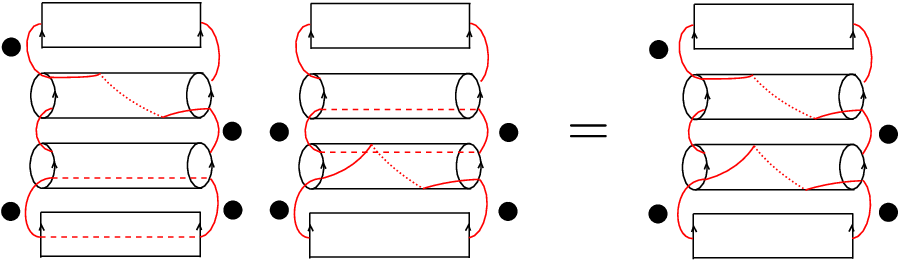
We envision the basis elements E⁡(s,c→)E(s,\vec{c}) as single diagrams, called basis diagrams, comprised of non-constant solid strands in [0,1]×𝒵⁡(n)[0,1]\times\mathcal{Z}(n) (corresponding to the non-constant strands of ss) together with pairs of constant dashed strands in [0,1]×𝒵⁡(n)[0,1]\times\mathcal{Z}(n) whose endpoints are matched by MM (corresponding to the constant strands of ss which lead to choices for 𝐢\mathbf{i} in the sum for EE). In this way, a single pair of matched dashed strands indicates a sum of two strands diagrams. In each diagram we remove one of the two dashed strands and replace the other one with a solid strand. See Figure 12 for an illustration.

Refer to caption
Figure 12. Dotted-line pictures of basis elements of 𝒜⁡(n,k,𝒮)\mathcal{A}(n,k,\mathcal{S}).

The concatenation of basis elements b1b_{1} and b2∈𝒜⁡(n,k,𝒮)b_{2}\in\mathcal{A}(n,k,\mathcal{S}) can be described pictorially in terms of basis diagrams. When a pair of dashed strands matches another pair of dashed strands, then they appear in the basis diagram of b1​b2b_{1}b_{2} as well. When a pair of dashed strands matches a single solid strand, then the dashed strand matched with the solid strand is treated as solid, whereas the other one disappears (see Figure 13). Finally, whenever a solid strand (or a pair of matched strands) of b1b_{1} does not match any (solid or pair of dashed) strands of b2b_{2}, the product b1​b2b_{1}b_{2} vanishes.

Refer to caption
Figure 13. Multiplying basis elements of 𝒜⁡(n,k,𝒮)\mathcal{A}(n,k,\mathcal{S}).

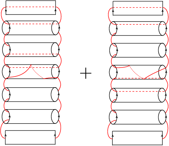
Considering basis diagrams makes the visual interpretation of the differential clear as well. Viewing aa as a single basis diagram of solid and dashed strands as above, we express b=∂ab=\partial a as a sum of crossing resolutions of aa. Terms coming from resolving a crossing between solid strands clearly give further basis diagrams (the orientation-preserving property of strands ensures that a non-constant strand cannot suddenly become constant after a crossing resolution). Meanwhile, crossings between solid and dashed strands can only contribute terms when the intersecting dashed strand is considered solid, and its matched partner is missing, giving a basis diagram after resolution with one fewer pair of dashed lines (note that after resolution, the formerly constant solid strand is no longer constant, and neither is the other solid strand). See Figure 14 for an illustration. This argument indicates that 𝒜⁡(n,k,𝒮)\mathcal{A}(n,k,\mathcal{S}) should inherit the differential of 𝒜~​(n,k,𝒮)\widetilde{\mathcal{A}}(n,k,\mathcal{S}), which we prove using the following sequence of lemmas whose proofs are structurally very similar to each other. We will continue to use the notations of Definition 4.7 throughout.

Refer to caption
Figure 14. Differentiating basis elements of 𝒜⁡(n,k,𝒮)\mathcal{A}(n,k,\mathcal{S}).
Lemma 4.13.

For any a∈𝒜⁡(n,k,𝒮)a\in\mathcal{A}(n,k,\mathcal{S}), we have ∂jca∈𝒜⁡(n,k,𝒮)\partial_{j}^{c}a\in\mathcal{A}(n,k,\mathcal{S}) for all j∈[1,n]j\in[1,n].

Proof.

By linearity, we can suppose that a=E⁡(s,c→)a=E(s,\vec{c}) where s⁡(0)∩M⁡(s⁡(0))=s⁡(1)∩M⁡(s⁡(1))=∅s(0)\cap M(s(0))=s(1)\cap M(s(1))=\varnothing. If ss has any non-constant strands on the backbone Sj1S^{1}_{j}, then all constant strands of ss remain constant in any summand of ∂jc(s,c→)\partial_{j}^{c}(s,\vec{c}). In such a case, 𝐈\mathbf{I} is the set of starting points for constant strands in any summand of ∂jc(s,c→)\partial_{j}^{c}(s,\vec{c}). Thus, we have

∂jc(E⁡(s,c→))\displaystyle\partial_{j}^{c}(E(s,\vec{c})) =∂jc(∑𝐢⊂𝐈(s𝐢,c→))\displaystyle=\partial_{j}^{c}\left(\sum_{\mathbf{i}\subset\mathbf{I}}(s_{\mathbf{i}},\vec{c})\right)
=∑𝐢⊂𝐈∂jc(s𝐢,c→)\displaystyle=\sum_{\mathbf{i}\subset\mathbf{I}}\partial_{j}^{c}(s_{\mathbf{i}},\vec{c})
=E⁡(∂jc(s,c→))∈𝒜⁡(n,k,𝒮).\displaystyle=E(\partial_{j}^{c}(s,\vec{c}))\in\mathcal{A}(n,k,\mathcal{S}).

Now we consider the case where ss has no strands of speeds greater than zero on the backbone Sj1S^{1}_{j}. If s𝐢s_{\mathbf{i}} has no strands at all on Sj1S^{1}_{j} for all 𝐢⊂𝐈\mathbf{i}\subset\mathbf{I}, then every term ∂jc(s𝐢,c→)\partial_{j}^{c}(s_{\mathbf{i}},\vec{c}) in the sum for ∂jcE⁡(s,c→)\partial_{j}^{c}E(s,\vec{c}) is zero. Similarly, if c→​(j)=0\vec{c}(j)=0, every term in the sum is zero as well. Thus, we can assume that c→​(j)=1\vec{c}(j)=1 and there is some 𝐢⊂𝐈\mathbf{i}\subset\mathbf{I} such that s𝐢s_{\mathbf{i}} has at least one constant strand on Sj1S^{1}_{j}. After replacing ss with some s𝐢s_{\mathbf{i}} if necessary, we can also assume that the number of (constant) strands of ss on Sj1S^{1}_{j} is maximal among elements of {s𝐢|𝐢⊂𝐈}\{s_{\mathbf{i}}\,|\,\mathbf{i}\subset\mathbf{I}\}. From here we consider two further subcases.

  1. (1)

    (One dashed strand and one loop) If ss contains only one constant strand on Sj1S^{1}_{j}, with starting (and ending) basepoint zj∘z_{j}^{\circ} (here ∘\circ can be a ++ or a −-), we compute as follows:

    ∂jcE⁡(s,c→)\displaystyle\partial_{j}^{c}E(s,\vec{c}) =∂jc∑𝐢⊂(𝐈∖{zj∘})((s𝐢,c→)+(s𝐢∪{zj∘},c→))\displaystyle=\partial_{j}^{c}\sum_{\mathbf{i}\subset\left(\mathbf{I}\setminus\left\{z_{j}^{\circ}\right\}\right)}\left((s_{\mathbf{i}},\vec{c})+(s_{\mathbf{i}\cup\left\{z_{j}^{\circ}\right\}},\vec{c})\right)
    =∑𝐢⊂(𝐈∖{zj∘})(∂jc(s𝐢,c→)+∂jc(s𝐢∪{zj∘},c→))\displaystyle=\sum_{\mathbf{i}\subset\left(\mathbf{I}\setminus\left\{z_{j}^{\circ}\right\}\right)}\left(\partial_{j}^{c}(s_{\mathbf{i}},\vec{c})+\partial_{j}^{c}(s_{\mathbf{i}\cup\left\{z_{j}^{\circ}\right\}},\vec{c})\right)
    =∑𝐢⊂(𝐈∖{zj∘})((s𝐢′,c→′)+0)\displaystyle=\sum_{\mathbf{i}\subset\left(\mathbf{I}\setminus\left\{z_{j}^{\circ}\right\}\right)}\left((s_{\mathbf{i}}^{\prime},\vec{c}\mkern 2.0mu\vphantom{c}^{\prime})+0\right)

    where s𝐢′s_{\mathbf{i}}^{\prime} and c→′\vec{c}\mkern 2.0mu\vphantom{c}^{\prime} are defined as in Definition 4.5. The zero term in the last line follows from the fact that s𝐢∪{zj∘}s_{\mathbf{i}\cup\left\{z_{j}^{\circ}\right\}} cannot have any strands on Sj1S^{1}_{j}. Meanwhile, the terms (s𝐢′,c→′)(s_{\mathbf{i}}^{\prime},\vec{c}\mkern 2.0mu\vphantom{c}^{\prime}) will be nonzero by assumption, and since s′s^{\prime} in Definition 4.5 replaces the formerly constant strand at zj∘z_{j}^{\circ} by one with speed 2 (but does not change any other strands), the set 𝐈∖{zj∘}\mathbf{I}\setminus\left\{z_{j}^{\circ}\right\} is precisely the set of starting basepoints of constant strands for s′s^{\prime}. Thus we have

    ∂jcE⁡(s,c→)=E⁡(s′,c→′)=E⁡(∂jc(s,c→))∈𝒜⁡(n,k,𝒮)\partial_{j}^{c}E(s,\vec{c})=E(s^{\prime},\vec{c}\mkern 2.0mu\vphantom{c}^{\prime})=E(\partial_{j}^{c}(s,\vec{c}))\in\mathcal{A}(n,k,\mathcal{S})

    just as in the case when we had non-constant strands.

  2. (2)

    (Two dashed strands and one loop) If ss contains two constant strands on Sj1S^{1}_{j}, with starting basepoints zj−,zj+z_{j}^{-},z_{j}^{+}, we begin in the same way:

    ∂jcE⁡(s,c→)\displaystyle\partial_{j}^{c}E(s,\vec{c}) =∂jc∑𝐢⊂(𝐈∖{zj−,zj+})((s𝐢,c→)+(s𝐢∪{zj−},c→)+(s𝐢∪{zj+},c→)+(s𝐢∪{zj−,zj+},c→))\displaystyle=\partial_{j}^{c}\sum_{\mathbf{i}\subset\left(\mathbf{I}\setminus\left\{z_{j}^{-},z_{j}^{+}\right\}\right)}\left((s_{\mathbf{i}},\vec{c})+(s_{\mathbf{i}\cup\left\{z_{j}^{-}\right\}},\vec{c})+(s_{\mathbf{i}\cup\left\{z_{j}^{+}\right\}},\vec{c})+(s_{\mathbf{i}\cup\left\{z_{j}^{-},z_{j}^{+}\right\}},\vec{c})\right)
    =∑𝐢⊂(𝐈∖{zj−,zj+})(∂jc(s𝐢,c→)+∂jc(s𝐢∪{zj−},c→)+∂jc(s𝐢∪{zj+},c→)+0)\displaystyle=\sum_{\mathbf{i}\subset\left(\mathbf{I}\setminus\left\{z_{j}^{-},z_{j}^{+}\right\}\right)}\left(\partial_{j}^{c}(s_{\mathbf{i}},\vec{c})+\partial_{j}^{c}(s_{\mathbf{i}\cup\left\{z_{j}^{-}\right\}},\vec{c})+\partial_{j}^{c}(s_{\mathbf{i}\cup\left\{z_{j}^{+}\right\}},\vec{c})+0\right)

    where we get the zero term using the same reasoning as before. Now we write ∂jc(s𝐢,c→)=(s𝐢−,c→′)+(s𝐢+,c→′)\partial_{j}^{c}(s_{\mathbf{i}},\vec{c})=(s_{\mathbf{i}}^{-},\vec{c}\mkern 2.0mu\vphantom{c}^{\prime})+(s_{\mathbf{i}}^{+},\vec{c}\mkern 2.0mu\vphantom{c}^{\prime}) where s𝐢±s_{\mathbf{i}}^{\pm} is the kk-strand defined by replacing the constant strand at zj±z_{j}^{\pm} by a new strand of speed 2, while maintaining the other strands (including the constant strand at zj∓z_{j}^{\mp}). We can then write our sum as

    ∂jcE⁡(s,c→)=∑𝐢⊂(𝐈∖{zj−,zj+})((s𝐢+,c→′)+(s𝐢∪{zj−}′,c→′)+(s𝐢−,c→′)+(s𝐢∪{zj+}′,c→′))\partial_{j}^{c}E(s,\vec{c})=\sum_{\mathbf{i}\subset\left(\mathbf{I}\setminus\left\{z_{j}^{-},z_{j}^{+}\right\}\right)}\left((s_{\mathbf{i}}^{+},\vec{c}\mkern 2.0mu\vphantom{c}^{\prime})+(s^{\prime}_{\mathbf{i}\cup\left\{z_{j}^{-}\right\}},\vec{c}\mkern 2.0mu\vphantom{c}^{\prime})+(s_{\mathbf{i}}^{-},\vec{c}\mkern 2.0mu\vphantom{c}^{\prime})+(s^{\prime}_{\mathbf{i}\cup\left\{z_{j}^{+}\right\}},\vec{c}\mkern 2.0mu\vphantom{c}^{\prime})\right)

    where s𝐢∪{zj±}′s^{\prime}_{\mathbf{i}\cup\left\{z_{j}^{\pm}\right\}} are defined as in Definition 4.5. The key point is to recognize that (s𝐢+,c→′)(s_{\mathbf{i}}^{+},\vec{c}\mkern 2.0mu\vphantom{c}^{\prime}) and (s𝐢∪{zj−}′,c→′)(s^{\prime}_{\mathbf{i}\cup\left\{z_{j}^{-}\right\}},\vec{c}\mkern 2.0mu\vphantom{c}^{\prime}) are complementary in the sense that both have a strand of speed 2 starting and ending at zj+z_{j}^{+}, and indeed have the same strands everywhere except that (s𝐢+,c→′)(s_{\mathbf{i}}^{+},\vec{c}\mkern 2.0mu\vphantom{c}^{\prime}) has a constant strand at zj−z_{j}^{-}, while (s𝐢∪{zj−}′,c→′)(s^{\prime}_{\mathbf{i}\cup\left\{z_{j}^{-}\right\}},\vec{c}\mkern 2.0mu\vphantom{c}^{\prime}) has a constant strand at zj−1+=M⁡(zj−)z_{j-1}^{+}=M(z_{j}^{-}). This reasoning implies that

    ∑𝐢⊂(𝐈∖{zj−,zj+})((s𝐢+,c→′)+(s𝐢∪{zj−}′,c→′))=∑𝐢⊂(𝐈∖{zj+})(s𝐢+,c→′)\sum_{\mathbf{i}\subset\left(\mathbf{I}\setminus\left\{z_{j}^{-},z_{j}^{+}\right\}\right)}\left((s_{\mathbf{i}}^{+},\vec{c}\mkern 2.0mu\vphantom{c}^{\prime})+(s^{\prime}_{\mathbf{i}\cup\left\{z_{j}^{-}\right\}},\vec{c}\mkern 2.0mu\vphantom{c}^{\prime})\right)=\sum_{\mathbf{i}\subset\left(\mathbf{I}\setminus\left\{z_{j}^{+}\right\}\right)}(s^{+}_{\mathbf{i}},\vec{c}\mkern 2.0mu\vphantom{c}^{\prime})

    and similarly we have

    ∑𝐢⊂(𝐈∖{zj−,zj+})((s𝐢−,c→′)+(s𝐢∪{zj+}′,c→′))=∑𝐢⊂(𝐈∖{zj−})(s𝐢−,c→′).\sum_{\mathbf{i}\subset\left(\mathbf{I}\setminus\left\{z_{j}^{-},z_{j}^{+}\right\}\right)}\left((s_{\mathbf{i}}^{-},\vec{c}\mkern 2.0mu\vphantom{c}^{\prime})+(s^{\prime}_{\mathbf{i}\cup\left\{z_{j}^{+}\right\}},\vec{c}\mkern 2.0mu\vphantom{c}^{\prime})\right)=\sum_{\mathbf{i}\subset\left(\mathbf{I}\setminus\left\{z_{j}^{-}\right\}\right)}(s^{-}_{\mathbf{i}},\vec{c}\mkern 2.0mu\vphantom{c}^{\prime}).

    Since 𝐈∖{zj±}\mathbf{I}\setminus\left\{z_{j}^{\pm}\right\} is the set of constant strand starting points for s±s^{\pm}, we have

    ∂jcE⁡(s,c→)\displaystyle\partial_{j}^{c}E(s,\vec{c}) =∑𝐢⊂(𝐈∖{zj+})(s𝐢+,c→′)+∑𝐢⊂(𝐈∖{zj−})(s𝐢−,c→′)\displaystyle=\sum_{\mathbf{i}\subset\left(\mathbf{I}\setminus\left\{z_{j}^{+}\right\}\right)}(s^{+}_{\mathbf{i}},\vec{c}\mkern 2.0mu\vphantom{c}^{\prime})+\sum_{\mathbf{i}\subset\left(\mathbf{I}\setminus\left\{z_{j}^{-}\right\}\right)}(s^{-}_{\mathbf{i}},\vec{c}\mkern 2.0mu\vphantom{c}^{\prime})
    =E⁡(s+,c→′)+E⁡(s−,c→′)\displaystyle=E(s^{+},\vec{c}\mkern 2.0mu\vphantom{c}^{\prime})+E(s^{-},\vec{c}\mkern 2.0mu\vphantom{c}^{\prime})
    =E⁡(∂jc(s,c→))∈𝒜⁡(n,k,𝒮).\displaystyle=E(\partial_{j}^{c}(s,\vec{c}))\in\mathcal{A}(n,k,\mathcal{S}).

Thus in all cases we see that, after replacing ss with some s𝐢s_{\mathbf{i}} if necessary as described above,

(4.4) ∂jc(E⁡(s,c→))=E⁡(∂jc(s,c→))∈𝒜⁡(n,k,𝒮),\partial_{j}^{c}(E(s,\vec{c}))=E(\partial_{j}^{c}(s,\vec{c}))\in\mathcal{A}(n,k,\mathcal{S}),

proving the lemma. ∎

Lemma 4.14.

For any a∈𝒜⁡(n,k,𝒮)a\in\mathcal{A}(n,k,\mathcal{S}), we have ∂j0a∈𝒜⁡(n,k,𝒮)\partial_{j}^{0}a\in\mathcal{A}(n,k,\mathcal{S}) for all j∈[1,n]j\in[1,n].

Proof.

As in the proof of Lemma 4.13, we can suppose that a=E⁡(s,c→)a=E(s,\vec{c}) where s⁡(0)∩M⁡(s⁡(0))=s⁡(1)∩M⁡(s⁡(1))=∅s(0)\cap M(s(0))=s(1)\cap M(s(1))=\varnothing. If ∂j0(s𝐢,c→)=0\partial^{0}_{j}(s_{\mathbf{i}},\vec{c})=0 for all 𝐢⊂𝐈\mathbf{i}\subset\mathbf{I}, then we have ∂j0a=0∈𝒜⁡(n,k,𝒮)\partial^{0}_{j}a=0\in\mathcal{A}(n,k,\mathcal{S}) trivially. Thus it is enough to consider the case where there is some subset 𝐢⊂𝐈\mathbf{i}\subset\mathbf{I} such that ∂j0(s𝐢,c→)≠0\partial^{0}_{j}(s_{\mathbf{i}},\vec{c})\neq 0. By Lemma 4.9 we can replace ss by this s𝐢s_{\mathbf{i}} without changing aa, and so we may assume without loss of generality that ss itself satisfies ∂j0(s,c→)≠0\partial^{0}_{j}(s,\vec{c})\neq 0.

In particular, we may assume that ss contains two strands on the backbone Sj1S^{1}_{j} having unequal speeds p>qp>q. We now split into two further subcases:

  1. (1)

    q≠0q\neq 0 (Two solid strands): In this case, neither strand on Sj1S^{1}_{j} is constant, so every term in the sum ∂j0a=∑𝐢⊂𝐈(∂j0(s𝐢,c→))\partial^{0}_{j}a=\sum_{\mathbf{i}\subset\mathbf{I}}(\partial^{0}_{j}(s_{\mathbf{i}},\vec{c})) is nonzero, and is a sum of one term (if p−q=2p-q=2) or two terms (if p−q>2p-q>2) with non-constant strands. Furthermore, since ∂j0\partial^{0}_{j} does not affect any strand away from the backbone Sj1S^{1}_{j}, constant strands of ss remain constant in any summand of ∂j0(s,c→)\partial^{0}_{j}(s,\vec{c}). Thus the set 𝐈\mathbf{I} of constant strand starting points for ss is the set of constant strand starting points for any summand of ∂j0(s,c→)\partial^{0}_{j}(s,\vec{c}) in this case. For 𝐢⊂𝐈\mathbf{i}\subset\mathbf{I}, we may write ∂j0(s𝐢,c→)=(∂j0(s,c→))𝐢\partial^{0}_{j}(s_{\mathbf{i}},\vec{c})=(\partial^{0}_{j}(s,\vec{c}))_{\mathbf{i}}, so our sum becomes

    ∂j0a=∑𝐢⊂𝐈(∂j0(s,c→))𝐢=E⁡(∂j0(s,c→))∈𝒜⁡(n,k,𝒮),\partial^{0}_{j}a=\sum_{\mathbf{i}\subset\mathbf{I}}(\partial^{0}_{j}(s,\vec{c}))_{\mathbf{i}}=E(\partial^{0}_{j}(s,\vec{c}))\in\mathcal{A}(n,k,\mathcal{S}),

    extending ()𝐢()_{\mathbf{i}} linearly.

  2. (2)

    q=0q=0 (One dashed strand): In this case, ss has a constant strand on some basepoint zj∘∈Sj1z_{j}^{\circ}\in S^{1}_{j}, where ∘∈{+,−}\circ\in\{+,-\}. Thus for any 𝐢⊂𝐈\mathbf{i}\subset\mathbf{I} containing zj∘z_{j}^{\circ}, s𝐢s_{\mathbf{i}} does not contain this constant strand, so ∂j0(s𝐢,c→)=0\partial^{0}_{j}(s_{\mathbf{i}},\vec{c})=0. It follows that the only terms in the sum that matter are those that come from subsets not containing zj∘z_{j}^{\circ}. For such subsets 𝐢\mathbf{i}, we may again write ∂j0(s𝐢,c→)=(∂j0(s,c→))𝐢\partial^{0}_{j}(s_{\mathbf{i}},\vec{c})=(\partial^{0}_{j}(s,\vec{c}))_{\mathbf{i}}.

    Meanwhile, the terms in ∂j0(s,c→)\partial^{0}_{j}(s,\vec{c}) will contain strands of speeds p−1p-1 and 11 on Sj1S^{1}_{j}. There will be two such terms if p≠2p\neq 2 and one such term if p=2p=2. All other strands of ss are maintained. We cannot have p=1p=1 since the strands of ss end on distinct basepoints in s⁡(1)s(1). Thus, the set of constant strand starting points for ∂j0(s,c→)\partial^{0}_{j}(s,\vec{c}) is precisely 𝐈∖{zj∘}\mathbf{I}\setminus\left\{z_{j}^{\circ}\right\}. Altogether, we can write our sum as

    ∂j0a=∑𝐢⊂𝐈∖{zj∘}(∂j0(s𝐢,c→))=∑𝐢⊂(𝐈∖{zj∘})(∂j(s,c→))𝐢=E⁡(∂j0(s,c→))∈𝒜⁡(n,k,𝒮)\partial^{0}_{j}a=\sum_{\mathbf{i}\subset\mathbf{I}\setminus\left\{z_{j}^{\circ}\right\}}(\partial^{0}_{j}(s_{\mathbf{i}},\vec{c}))=\sum_{\mathbf{i}\subset(\mathbf{I}\setminus\left\{z_{j}^{\circ}\right\})}(\partial_{j}(s,\vec{c}))_{\mathbf{i}}=E(\partial^{0}_{j}(s,\vec{c}))\in\mathcal{A}(n,k,\mathcal{S})

    where we have again extended ()𝐢()_{\mathbf{i}} linearly.

As in Lemma 4.13, we have

(4.5) ∂j0(E⁡(s,c→))=E⁡(∂j0(s,c→))∈𝒜⁡(n,k,𝒮)\partial_{j}^{0}(E(s,\vec{c}))=E(\partial_{j}^{0}(s,\vec{c}))\in\mathcal{A}(n,k,\mathcal{S})

in all cases, again after replacing ss with some s𝐢s_{\mathbf{i}} if necessary, proving the lemma. ∎

Proposition 4.15.

The subspace 𝒜⁡(n,k,𝒮)\mathcal{A}(n,k,\mathcal{S}) of 𝒜~​(n,k,𝒮)\widetilde{\mathcal{A}}(n,k,\mathcal{S}) is preserved by the differential on 𝒜~​(n,k,𝒮)\widetilde{\mathcal{A}}(n,k,\mathcal{S}).

Proof.

Since ∂=∑j∈[1,n]∂jc+∂j0\partial=\sum_{j\in[1,n]}\partial_{j}^{c}+\partial_{j}^{0}, this proposition follows from Lemmas 4.13 and 4.14. ∎

4.5. Idempotents and the unit

At this point, we can almost say that 𝒜⁡(n,k,𝒮)\mathcal{A}(n,k,\mathcal{S}) is a differential algebra (we will see in Section 6 that it is in fact a dg algebra). One subtlety is that the unit of 𝒜~​(n,k,𝒮)\widetilde{\mathcal{A}}(n,k,\mathcal{S}) is not an element of 𝒜⁡(n,k,𝒮)\mathcal{A}(n,k,\mathcal{S}). However, 𝒜⁡(n,k,𝒮)\mathcal{A}(n,k,\mathcal{S}) has its own unit, which we define below.

Let BB be the set of basepoints in 𝒵⁡(n)\mathcal{Z}(n) as above, and let MM be the matching on BB. We write B/M:=B/(z∼M⁡(z))B/M:=B/(z\sim M(z)) and consider the quotient map q:B→B/Mq:B\rightarrow B/M. We can identify B/MB/M with [0,n][0,n] by sending {zi+,zi+1−}∈B/M\{z_{i}^{+},z_{i+1}^{-}\}\in B/M to the index i∈[0,n]i\in[0,n].

Let 𝐱\mathbf{x} be a kk-element subset 𝐱\mathbf{x} of B/M≅[0,n]B/M\cong[0,n], i.e. an element of V⁡(n,k)V(n,k) in the notation of Definition 2.2 (we will resume using this notation below). Following Lipshitz–Ozsváth–Thurston, we will call a subset 𝐒⊂B\mathbf{S}\subset B a section of 𝐱\mathbf{x} if 𝐒\mathbf{S} is the image of a section of the quotient map qq over 𝐱\mathbf{x}.

Definition 4.16.

For 𝐱∈V⁡(n,k)\mathbf{x}\in V(n,k), let 𝐉𝐱\mathbf{J}_{\mathbf{x}} be the element E⁡(Const𝐒,0→)E(\const_{\mathbf{S}},\vec{0}) of 𝒜⁡(n,k,𝒮)\mathcal{A}(n,k,\mathcal{S}) where 𝐒\mathbf{S} is any section of 𝐱\mathbf{x} and Const𝐒\const_{\mathbf{S}} is the kk-strand of constant strands at each basepoint in 𝐒\mathbf{S}. Note that this definition is independent of the choice of 𝐒\mathbf{S} by Lemma 4.9. Define

1𝒜⁡(n,k,𝒮):=∑𝐱∈V⁡(n,k)𝐉𝐱.1_{\mathcal{A}(n,k,\mathcal{S})}:=\sum_{\mathbf{x}\in V(n,k)}\mathbf{J}_{\mathbf{x}}.

A section 𝐒\mathbf{S} of 𝐱\mathbf{x} can always be chosen by the rule that i∈𝐱i\in\mathbf{x} if and only if zi+∈𝐒z_{i}^{+}\in\mathbf{S}. Regardless of the choice of section, however, the element 𝐉𝐱\mathbf{J}_{\mathbf{x}} is visually interpreted as the diagram consisting of a constant dashed strand at each point of q−1​(𝐱)⊂Bq^{-1}(\mathbf{x})\subset B. The elements 𝐉𝐱\mathbf{J}_{\mathbf{x}} for 𝐱∈V⁡(n,k)\mathbf{x}\in V(n,k) constitute a set of pairwise orthogonal idempotents in 𝒜⁡(n,k,𝒮)\mathcal{A}(n,k,\mathcal{S}).

Proposition 4.17.

The element 1𝒜⁡(n,k,𝒮)1_{\mathcal{A}(n,k,\mathcal{S})} is an identity element for 𝒜⁡(n,k,𝒮)\mathcal{A}(n,k,\mathcal{S}).

Proof.

Let E⁡(s,c→)E(s,\vec{c}) denote a standard basis element of 𝒜⁡(n,k,𝒮)\mathcal{A}(n,k,\mathcal{S}). Let 𝐲,𝐳∈V⁡(n,k)\mathbf{y},\mathbf{z}\in V(n,k) denote the images of q⁡(s⁡(0))q(s(0)) and q⁡(s⁡(1))q(s(1)) respectively under the identification of B/MB/M with [0,n][0,n]. Note that, if 𝐱≠𝐲\mathbf{x}\neq\mathbf{y}, then 𝐉𝐱⋅E⁡(s,c→)=0\mathbf{J}_{\mathbf{x}}\cdot E(s,\vec{c})=0 because none of the summands of 𝐉𝐱\mathbf{J}_{\mathbf{x}} and E⁡(s,c→)E(s,\vec{c}) are concatenable, while 𝐉𝐲⋅E⁡(s,c→)=E⁡(s,c→)\mathbf{J}_{\mathbf{y}}\cdot E(s,\vec{c})=E(s,\vec{c}) (see the proof of Proposition 4.12 where it is shown that E⁡(t,d→)⋅E⁡(s,c→)=E⁡(t⋅s,d→+c→)E(t,\vec{d})\cdot E(s,\vec{c})=E(t\cdot s,\vec{d}+\vec{c}) after tt and ss are chosen appropriately). Similarly, E⁡(s,c→)⋅𝐉𝐱=0E(s,\vec{c})\cdot\mathbf{J}_{\mathbf{x}}=0 for 𝐱≠𝐳\mathbf{x}\neq\mathbf{z}, while E⁡(s,c→)⋅𝐉𝐳=E⁡(s,c→)E(s,\vec{c})\cdot\mathbf{J}_{\mathbf{z}}=E(s,\vec{c}). Thus we have

1𝒜⁡(n,k,𝒮)⋅E⁡(s,c→)=𝐉𝐲⋅E⁡(s,c→)+∑𝐱≠𝐲𝐉𝐱⋅E⁡(s,c→)=E⁡(s,c→),\displaystyle 1_{\mathcal{A}(n,k,\mathcal{S})}\cdot E(s,\vec{c})=\mathbf{J}_{\mathbf{y}}\cdot E(s,\vec{c})+\sum_{\mathbf{x}\neq\mathbf{y}}\mathbf{J}_{\mathbf{x}}\cdot E(s,\vec{c})=E(s,\vec{c}),
E⁡(s,c→)⋅1𝒜⁡(n,k,𝒮)=E⁡(s,c→)⋅𝐉𝐳+∑𝐱≠𝐳E⁡(s,c→)⋅𝐉𝐱=E⁡(s,c→).\displaystyle E(s,\vec{c})\cdot 1_{\mathcal{A}(n,k,\mathcal{S})}=E(s,\vec{c})\cdot\mathbf{J}_{\mathbf{z}}+\sum_{\mathbf{x}\neq\mathbf{z}}E(s,\vec{c})\cdot\mathbf{J}_{\mathbf{x}}=E(s,\vec{c}).

∎

We see that 𝒜⁡(n,k,𝒮)\mathcal{A}(n,k,\mathcal{S}) is a differential algebra over 𝔽2\mathbb{F}_{2} (gradings will be discussed in Section 6). Moreover, 𝒜⁡(n,k,𝒮)\mathcal{A}(n,k,\mathcal{S}) can be viewed as an algebra over the idempotent ring 𝐈⁡(n,k)=𝔽2V⁡(n,k)\mathbf{I}(n,k)=\mathbb{F}_{2}^{V(n,k)} via the ring homomorphism sending the indicator function of 𝐱∈V⁡(n,k)\mathbf{x}\in V(n,k) to 𝐉𝐱∈𝒜⁡(n,k,𝒮)\mathbf{J}_{\mathbf{x}}\in\mathcal{A}(n,k,\mathcal{S}), and we have a natural splitting

(4.6) 𝒜⁡(n,k,𝒮)=⨁𝐱,𝐲∈V⁡(n,k)𝐉𝐱​𝒜​(n,k,𝒮)​𝐉𝐲\mathcal{A}(n,k,\mathcal{S})=\bigoplus_{\mathbf{x},\mathbf{y}\in V(n,k)}{\mathbf{J}_{\mathbf{x}}}\mathcal{A}(n,k,\mathcal{S}){\mathbf{J}_{\mathbf{y}}}

(see [MMW19, Lemma A.17 in Appendix A] for more details).

Each element of the basis for 𝒜⁡(n,k,𝒮)\mathcal{A}(n,k,\mathcal{S}) from Definition 4.11 is homogeneous with respect to the decomposition of (4.6). The basis element E⁡(s,c→)E(s,\vec{c}) lies in 𝐉𝐱​𝒜​(n,k,𝒮)​𝐉𝐲\mathbf{J}_{\mathbf{x}}\mathcal{A}(n,k,\mathcal{S}){\mathbf{J}_{\mathbf{y}}} if and only if 𝐱\mathbf{x} and 𝐲\mathbf{y} are the projections of s⁡(0),s⁡(1)⊂Bs(0),s(1)\subset B to kk-element subsets of (B/M)≅[0,n](B/M)\cong[0,n] respectively (in other words, 𝐱\mathbf{x} and 𝐲\mathbf{y} are the unique I-states such that s⁡(0)s(0) is a section of 𝐱\mathbf{x} and s⁡(1)s(1) is a section of 𝐲\mathbf{y}). Thus, we have the following lemma.

Lemma 4.18.

Let 𝐱,𝐲∈V⁡(n,k)\mathbf{x},\mathbf{y}\in V(n,k). An 𝔽2\mathbb{F}_{2}-basis of the summand 𝐉𝐱​𝒜​(n,k,𝒮)​𝐉𝐲{\mathbf{J}_{\mathbf{x}}}\mathcal{A}(n,k,\mathcal{S}){\mathbf{J}_{\mathbf{y}}} of 𝒜⁡(n,k,𝒮)\mathcal{A}(n,k,\mathcal{S}) consists of all standard basis elements of 𝒜⁡(n,k,𝒮)\mathcal{A}(n,k,\mathcal{S}) of the form E⁡(s,c→)E(s,\vec{c}), where s⁡(0)s(0) and s⁡(1)s(1) are sections of 𝐱\mathbf{x} and 𝐲\mathbf{y} respectively.

4.6. Far states and the strands algebra

Recall that for 𝐱,𝐲∈V⁡(n,k)\mathbf{x},\mathbf{y}\in V(n,k) that are “far” in the sense of Definition 2.12, we have 𝐈𝐱​ℬ​(n,k,𝒮)​𝐈𝐲=0\mathbf{I}_{\mathbf{x}}\mathcal{B}(n,k,\mathcal{S})\mathbf{I}_{\mathbf{y}}=0. Below we prove a similar result for the strands algebra.

Lemma 4.19.

Let 𝐱,𝐲∈V⁡(n,k)\mathbf{x},\mathbf{y}\in V(n,k). If 𝐱,𝐲\mathbf{x},\mathbf{y} are far, then 𝐉𝐱​𝒜​(n,k,𝒮)​𝐉𝐲=0\mathbf{J}_{\mathbf{x}}\mathcal{A}(n,k,\mathcal{S})\mathbf{J}_{\mathbf{y}}=0.

Proof.

We will show the contrapositive. Let 𝐱={x1<⋯<xk}\mathbf{x}=\left\{x_{1}<\cdots<x_{k}\right\} and 𝐲={y1<⋯<yk}\mathbf{y}=\left\{y_{1}<\cdots<y_{k}\right\} and suppose that 𝐉𝐱​𝒜​(n,k,𝒮)​𝐉𝐲≠0\mathbf{J}_{\mathbf{x}}\mathcal{A}(n,k,\mathcal{S})\mathbf{J}_{\mathbf{y}}\neq 0. Then there exists a kk-strand ss from a section 𝐒\mathbf{S} of 𝐱\mathbf{x} to a section 𝐓\mathbf{T} of 𝐲\mathbf{y}, which in turn gives a bijection φ:𝐱→𝐲\varphi\colon\mathbf{x}\to\mathbf{y} with the property that for all a∈[1,k]a\in[1,k] we have

|φ⁡(xa)−xa|≤1.|\varphi(x_{a})-x_{a}|\leq 1.

We wish to show that this condition implies |ya−xa|≤1|y_{a}-x_{a}|\leq 1 for all aa as well (and hence 𝐱\mathbf{x} and 𝐲\mathbf{y} are not far). To prove that ya−xa≤1y_{a}-x_{a}\leq 1, assume by contradiction that the set {a∈[1,k]|ya−xa>1}\left\{a\in[1,k]\,\middle|\,y_{a}-x_{a}>1\right\} is non-empty, and let mm be its minimum. Then, for all b=1,…,m−1b=1,\ldots,m-1, we have that

φ⁡(xb)≤1+xb<ym.\varphi(x_{b})\leq 1+x_{b}<y_{m}.

Moreover, φ⁡(xm)−xm≤1<ym−xm\varphi(x_{m})-x_{m}\leq 1<y_{m}-x_{m}, so φ⁡(xm)<ym\varphi(x_{m})<y_{m} too. Then φ\varphi is injective from {x1,…,xm}\left\{x_{1},\ldots,x_{m}\right\} to {y1,…,ym−1}\left\{y_{1},\ldots,y_{m-1}\right\}, which is a contradiction. To prove that ya−xa≥−1y_{a}-x_{a}\geq-1, we can apply the same reasoning to the maximum of the set {a∈[1,k]|ya−xa<−1}\left\{a\in[1,k]\,\middle|\,y_{a}-x_{a}<-1\right\}. Thus we must have that |ya−xa|≤1|y_{a}-x_{a}|\leq 1, so 𝐱\mathbf{x} and 𝐲\mathbf{y} are not far. ∎

4.7. Idempotent-truncated strands algebras

As in [MMW19, Section 3.4], one can define truncated versions of 𝒜⁡(n,k,𝒮)\mathcal{A}(n,k,\mathcal{S}) (see also [OSz18, Section 12]).

Definition 4.20.

For 0≤k≤n0\leq k\leq n, define 𝒜r​(n,k,𝒮)\mathcal{A}_{r}(n,k,\mathcal{S}) to be

(∑𝐱:0∉𝐱𝐉𝐱)𝒜(n,k,𝒮)(∑𝐱:0∉𝐱𝐉𝐱).\bigg(\sum_{\mathbf{x}:0\notin\mathbf{x}}\mathbf{J}_{\mathbf{x}}\bigg)\mathcal{A}(n,k,\mathcal{S})\bigg(\sum_{\mathbf{x}:0\notin\mathbf{x}}\mathbf{J}_{\mathbf{x}}\bigg).

Similarly, define 𝒜l​(n,k,𝒮)\mathcal{A}_{l}(n,k,\mathcal{S}) to be

(∑𝐱:n∉𝐱𝐉𝐱)𝒜(n,k,𝒮)(∑𝐱:n∉𝐱𝐉𝐱).\bigg(\sum_{\mathbf{x}:n\notin\mathbf{x}}\mathbf{J}_{\mathbf{x}}\bigg)\mathcal{A}(n,k,\mathcal{S})\bigg(\sum_{\mathbf{x}:n\notin\mathbf{x}}\mathbf{J}_{\mathbf{x}}\bigg).

For 0≤k≤n−10\leq k\leq n-1, define 𝒜′​(n,k,𝒮)\mathcal{A}^{\prime}(n,k,\mathcal{S}) to be

(∑𝐱:0,n∉𝐱𝐉𝐱)𝒜(n,k,𝒮)(∑𝐱:0,n∉𝐱𝐉𝐱).\bigg(\sum_{\mathbf{x}:0,n\notin\mathbf{x}}\mathbf{J}_{\mathbf{x}}\bigg)\mathcal{A}(n,k,\mathcal{S})\bigg(\sum_{\mathbf{x}:0,n\notin\mathbf{x}}\mathbf{J}_{\mathbf{x}}\bigg).

As with the truncations of ℬ⁡(n,k,𝒮)\mathcal{B}(n,k,\mathcal{S}), one can also describe these algebras in terms of full subcategories of the dg category corresponding to 𝒜⁡(n,k,𝒮)\mathcal{A}(n,k,\mathcal{S}); see [MMW19, Definition 3.16].

In fact, as with 𝒜⁡(n,k,𝒮)\mathcal{A}(n,k,\mathcal{S}), the truncated algebras are special cases of strands algebras for chord diagrams that will be defined in [MR]. We describe these diagrams below.

Definition 4.21.

We define the chord diagram 𝒵r​(n)\mathcal{Z}_{r}(n) to be (𝒵r​(n),B,M)(\mathcal{Z}_{r}(n),B,M) where

𝒵r​(n):=S1⊔⋯⊔S1⊔[0,1].\mathcal{Z}_{r}(n):=S^{1}\sqcup\cdots\sqcup S^{1}\sqcup[0,1].

For i=2,…,ni=2,\ldots,n, let zi−:=[0]∈Si1z_{i}^{-}:=[0]\in S^{1}_{i} and zi+:=[1]∈Si1z_{i}^{+}:=[1]\in S^{1}_{i} be two distinct basepoints in Si1S^{1}_{i}. We also fix points z1+∈S11z_{1}^{+}\in S^{1}_{1} and zn+1−∈Int⁡([0,1]n+1)z_{n+1}^{-}\in\Int([0,1]_{n+1}). We define a matching MM on the set of basepoints B={z1+,z2±,…,zn±,zn+1−}B=\left\{z_{1}^{+},z_{2}^{\pm},\ldots,z_{n}^{\pm},z_{n+1}^{-}\right\} by matching zi+z_{i}^{+} with zi+1−z_{i+1}^{-}, i.e.,

M⁡(zi+)=zi+1−.M(z_{i}^{+})=z_{i+1}^{-}.

We define 𝒵l​(n)\mathcal{Z}_{l}(n) and 𝒵′​(n)\mathcal{Z}^{\prime}(n) similarly, with

𝒵l​(n):=[0,1]⊔S1⊔⋯⊔S1\mathcal{Z}_{l}(n):=[0,1]\sqcup S^{1}\sqcup\cdots\sqcup S^{1}

and

𝒵′​(n):=S1⊔⋯⊔S1.\mathcal{Z}^{\prime}(n):=S^{1}\sqcup\cdots\sqcup S^{1}.

Both ℱ​(𝒵r​(n))\mathcal{F}(\mathcal{Z}_{r}(n)) and ℱ​(𝒵l​(n))\mathcal{F}(\mathcal{Z}_{l}(n)) are a connected genus-zero sutured surface with n+1n+1 boundary components. One boundary component has two sutures; the rest have no sutures and are contained in S+S_{+}. The sutured surface ℱ​(𝒵′​(n))\mathcal{F}(\mathcal{Z}^{\prime}(n)) is a connected genus-zero surface with n+1n+1 boundary components and no sutures. All boundary components are contained in S+S^{+} except the outermost one, which is contained in S−S^{-}.

The chord diagrams 𝒵r​(3)\mathcal{Z}_{r}(3), 𝒵l​(3)\mathcal{Z}_{l}(3), and 𝒵′​(3)\mathcal{Z}^{\prime}(3) and the sutured surfaces ℱ​(𝒵r​(3))\mathcal{F}(\mathcal{Z}_{r}(3)), ℱ​(𝒵l​(3))\mathcal{F}(\mathcal{Z}_{l}(3)), and ℱ​(𝒵′​(3))\mathcal{F}(\mathcal{Z}^{\prime}(3)) are shown in Figure 15.

Refer to caption
Figure 15. The chord diagrams 𝒵l​(3)\mathcal{Z}_{l}(3), 𝒵r​(3)\mathcal{Z}_{r}(3), and 𝒵′​(3)\mathcal{Z}^{\prime}(3), and the sutured surfaces ℱ​(𝒵r​(3))\mathcal{F}(\mathcal{Z}_{r}(3)), ℱ​(𝒵l​(3))\mathcal{F}(\mathcal{Z}_{l}(3)), and ℱ​(𝒵′​(3))\mathcal{F}(\mathcal{Z}^{\prime}(3)).

5. Structure of the strands algebras

5.1. Notation and explicit bases for summands of 𝒜⁡(n,k,𝒮)\mathcal{A}(n,k,\mathcal{S})

As mentioned below Definition 4.1, a kk-strand can be described entirely by specifying the starting points and (constant) speeds of each strand. When we pass to the subalgebra 𝒜⁡(n,k,𝒮)\mathcal{A}(n,k,\mathcal{S}) within 𝒜~​(n,k,𝒮)\widetilde{\mathcal{A}}(n,k,\mathcal{S}), we treat constant strands somewhat differently from non-constant strands, but basis elements E⁡(s,c→)E(s,\vec{c}) should still be determined by starting points and speeds of each strand of ss (together with c→\vec{c}), where a speed of zero corresponds visually to a dashed strand rather than a solid strand.

Because the majority of results in this paper hinge upon the splitting

𝒜⁡(n,k,𝒮)≅⨁𝐱,𝐲∈V⁡(n,k)𝐉𝐱​𝒜​(n,k,𝒮)​𝐉𝐲,\mathcal{A}(n,k,\mathcal{S})\cong\bigoplus_{\mathbf{x},\mathbf{y}\in V(n,k)}\mathbf{J}_{\mathbf{x}}\mathcal{A}(n,k,\mathcal{S}){\mathbf{J}_{\mathbf{y}}},

we allow our notation to take the starting idempotent 𝐱\mathbf{x} as a given. That is, given a starting idempotent, we seek a notation that allows an immediate combinatorial and visual grasp of any given basis element E⁡(s,c→)E(s,\vec{c}) for any section s⁡(0)s(0) of 𝐱\mathbf{x}. With all of this in mind, we present the following definition starting from pairs (s,c→)(s,\vec{c}) in the pre-strands algebra.

Definition 5.1.

Suppose (s,c→)∈𝒜~​(n,k,𝒮)(s,\vec{c})\in\widetilde{\mathcal{A}}(n,k,\mathcal{S}). Let Ar⁡(s,c→)\Ar(s,\vec{c}) denote the following combination of a square-free monomial in variables CiC_{i} for i∈𝒮i\in\mathcal{S} together with an array of vectors:

Ar(s,c→):=∏i∈𝒮Cic→​(i)(p1q1)1(p2q2)2⋯(pnqn)n\Ar(s,\vec{c}):=\prod_{i\in\mathcal{S}}C_{i}^{\vec{c}(i)}\left(\begin{matrix}p_{1}\\ q_{1}\end{matrix}\right)_{1}\left(\begin{matrix}p_{2}\\ q_{2}\end{matrix}\right)_{2}\cdots\left(\begin{matrix}p_{n}\\ q_{n}\end{matrix}\right)_{n}

where each pi,qip_{i},q_{i} is defined as follows.

  • •

    If zi−z_{i}^{-} is the starting point of a non-constant strand sas_{a} of ss, then pip_{i} is the (constant) speed of this strand; otherwise we set pip_{i} equal to 00.

  • •

    if zi+z_{i}^{+} is the starting point of a non-constant strand sbs_{b} of ss, then qiq_{i} is the (constant) speed of this strand; otherwise we set qiq_{i} equal to 00.

We may also omit columns of all zeros from the array. In particular the following notation will be used often:

(5.1) (pq)i:=(00)1⋯(00)i−1(pq)i(00)i+1⋯(00)n.\left(\begin{matrix}p\\ q\end{matrix}\right)_{i}\quad:=\quad\left(\begin{matrix}0\\ 0\end{matrix}\right)_{1}\cdots\left(\begin{matrix}0\\ 0\end{matrix}\right)_{i-1}\left(\begin{matrix}p\\ q\end{matrix}\right)_{i}\left(\begin{matrix}0\\ 0\end{matrix}\right)_{i+1}\cdots\left(\begin{matrix}0\\ 0\end{matrix}\right)_{n}.

Recall that we have defined our circles Si1S^{1}_{i} and basepoints zi±z_{i}^{\pm} so that our speeds are integers, and a speed of 2 indicates a degree one map to the circle. In particular, a strand starts and ends at the same basepoint if and only if its speed is even.

Lemma 5.2.

Fix some starting idempotent 𝐱∈V⁡(n,k)\mathbf{x}\in V(n,k). For any two basis elements (s,c→)(s,\vec{c}) and (s′,c→′)(s^{\prime},\vec{c}\mkern 2.0mu\vphantom{c}^{\prime}) of 𝐉𝐱​𝒜~​(n,k,𝒮)\mathbf{J}_{\mathbf{x}}\widetilde{\mathcal{A}}(n,k,\mathcal{S}) with s⁡(0)∩M⁡(s⁡(0))=s⁡(1)∩M⁡(s⁡(1))=∅s(0)\cap M(s(0))=s(1)\cap M(s(1))=\varnothing and s′​(0)∩M⁡(s′​(0))=s′​(1)∩M⁡(s′​(1))=∅s^{\prime}(0)\cap M(s^{\prime}(0))=s^{\prime}(1)\cap M(s^{\prime}(1))=\varnothing, we have E⁡(s,c→)=E⁡(s′,c→′)E(s,\vec{c})=E(s^{\prime},\vec{c}\mkern 2.0mu\vphantom{c}^{\prime}) if and only if Ar⁡(s,c→)=Ar⁡(s′,c→′)\Ar(s,\vec{c})=\Ar(s^{\prime},\vec{c}\mkern 2.0mu\vphantom{c}^{\prime}).

Proof.

It is clear that if c→≠c→′\vec{c}\neq\vec{c}\mkern 2.0mu\vphantom{c}^{\prime}, then we have both E⁡(s,c→)≠E⁡(s′,c→′)E(s,\vec{c})\neq E(s^{\prime},\vec{c}\mkern 2.0mu\vphantom{c}^{\prime}) and Ar⁡(s,c→)≠Ar⁡(s′,c→′)\Ar(s,\vec{c})\neq\Ar(s^{\prime},\vec{c}\mkern 2.0mu\vphantom{c}^{\prime}). If c→=c→′\vec{c}=\vec{c}\mkern 2.0mu\vphantom{c}^{\prime}, Lemma 4.9 shows that E⁡(s,c→)=E⁡(s′,c→′)E(s,\vec{c})=E(s^{\prime},\vec{c}\mkern 2.0mu\vphantom{c}^{\prime}) if and only if s′=s𝐢s^{\prime}=s_{\mathbf{i}} for some 𝐢⊂𝐈\mathbf{i}\subset\mathbf{I}, where 𝐈\mathbf{I} is the set of basepoints that are starting points for constant strands of ss as usual.

We claim that s′=s𝐢s^{\prime}=s_{\mathbf{i}} for some 𝐢⊂𝐈\mathbf{i}\subset\mathbf{I} if and only if Ar⁡(s,c→)=Ar⁡(s′,c→)\Ar(s,\vec{c})=\Ar(s^{\prime},\vec{c}). Indeed if s′=s𝐢s^{\prime}=s_{\mathbf{i}}, then the only difference between ss and s′s^{\prime} is the placement of certain constant strands, which the notation of Definition 5.1 ignores.

Conversely, if Ar⁡(s,c→)=Ar⁡(s′,c→)\Ar(s,\vec{c})=\Ar(s^{\prime},\vec{c}), the nonzero entries of the arrays demand that ss and s′s^{\prime} have the same non-constant strands, so that they (possibly) differ only in the placement of their constant strands. Then since s⁡(0)s(0) and s′​(0)s^{\prime}(0) are both sections of 𝐱\mathbf{x}, we must have s′=s𝐢s^{\prime}=s_{\mathbf{i}} for some 𝐢⊂𝐈\mathbf{i}\subset\mathbf{I}. ∎

Lemma 5.2 shows that Ar⁡(s,c→)\Ar(s,\vec{c}) descends to a well-defined notation for basis elements E⁡(s,c→)E(s,\vec{c}) in 𝐉𝐱​𝒜​(n,k,𝒮)\mathbf{J}_{\mathbf{x}}\mathcal{A}(n,k,\mathcal{S}) once 𝐱\mathbf{x} has been fixed. Notice that an entry of zero in Ar⁡(s,c→)\Ar(s,\vec{c}) can mean two different things for the corresponding kk-strand ss—it can mean that there is no strand at all at the given basepoint, or it can mean that there is a constant (i.e. speed 0) strand at the given basepoint. In particular, the case qi=pi+1=0q_{i}=p_{i+1}=0 can mean there are no strands present at all, or that there is a single constant strand starting at either zi+z_{i}^{+} or zi+1−z_{i+1}^{-}, but it cannot mean that there are constant strands at both zi+z_{i}^{+} and zi+1−z_{i+1}^{-} since we have s⁡(0)∩M⁡(s⁡(0))=∅s(0)\cap M(s(0))=\varnothing.

Lemma 5.2 views this ambiguity as a helpful feature of the notation due to the ambiguity inherent in Lemma 4.9. However, one might object that the notation alone does not distinguish between a constant strand starting point, an empty basepoint that is matched to a constant strand starting point, and an empty basepoint that is not matched to a constant strand starting point. (As an extreme example, every idempotent element 𝐉𝐱\mathbf{J}_{\mathbf{x}} is written as an array of all zeros, regardless of 𝐱\mathbf{x}.) To address this objection, we always work with a fixed starting I-state 𝐱\mathbf{x}, implying the existence (or lack thereof) of strands starting from certain matched pairs of basepoints. We summarize this point with the following remark.

Remark 5.3.

The notation of Definition 5.1 is only well-defined for basis elements of 𝐉𝐱​𝒜​(n,k,𝒮)\mathbf{J}_{\mathbf{x}}\mathcal{A}(n,k,\mathcal{S}) for some fixed beginning I-state 𝐱\mathbf{x}. It is therefore not helpful as a notation for general basis elements in 𝒜⁡(n,k,𝒮)\mathcal{A}(n,k,\mathcal{S}). For computations in this paper using this notation, we will focus on a single summand 𝐉𝐱​𝒜​(n,k,𝒮)\mathbf{J}_{\mathbf{x}}\mathcal{A}(n,k,\mathcal{S}) of 𝒜⁡(n,k,𝒮)\mathcal{A}(n,k,\mathcal{S}) at a time.

Visually, once we have fixed a starting I-state 𝐱\mathbf{x}, the notation Ci1⋯Cil(p1q1)1⋯(pnqn)nC_{i_{1}}\cdots C_{i_{l}}\left(\begin{matrix}p_{1}\\ q_{1}\end{matrix}\right)_{1}\cdots\left(\begin{matrix}p_{n}\\ q_{n}\end{matrix}\right)_{n} indicates a specific basis diagram in which solid strands are drawn according to their speeds (the placement of pip_{i} above qiq_{i} in the notation is a reminder that pip_{i} is the speed starting from the upper basepoint, while qiq_{i} starts from the lower basepoint). Constant dashed strands are drawn on any matched pair of basepoints that are contained in 𝐱\mathbf{x} but have no solid strands coming from them. Closed loops are drawn on any cylinder whose CiC_{i} variable appears in the monomial. See Figure 16 for an example.

Refer to caption
Figure 16. The basis element C2​C4​C5​(19)1​(00)2​(02)3​(00)4​(11)5C_{2}C_{4}C_{5}\binom{1}{9}_{1}\binom{0}{0}_{2}\binom{0}{2}_{3}\binom{0}{0}_{4}\binom{1}{1}_{5} of 𝒜⁡(5,6,𝒮)\mathcal{A}(5,6,\mathcal{S}), also denoted C2​C4​C5​(19)1​(02)3​(11)5C_{2}C_{4}C_{5}\binom{1}{9}_{1}\binom{0}{2}_{3}\binom{1}{1}_{5}, starting at the idempotent 𝐉𝐱\mathbf{J}_{\mathbf{x}} where 𝐱={0,1,2,3,4,5}\mathbf{x}=\{0,1,2,3,4,5\} and 𝒮⊂[1,5]\mathcal{S}\subset[1,5] contains {2,4,5}\{2,4,5\}.

It should be clear that only certain arrays can appear in valid basis elements for a given summand 𝐉𝐱​𝒜​(n,k,𝒮)\mathbf{J}_{\mathbf{x}}\mathcal{A}(n,k,\mathcal{S}) of the strands algebra. Furthermore, given a valid array, the ending idempotent of the corresponding strands algebra element is also determined. Visually all that is required is that no two solid strands start on matched basepoints, and that no two strands (whether solid or dashed) end on basepoints that are either the same or matched. The following lemma describes the precise combinatorics involved; see Figure 17 for reference.

Refer to caption
Figure 17. Reference diagram for the proof of Lemma 5.4.
Lemma 5.4.

For 𝐱∈V⁡(n,k)\mathbf{x}\in V(n,k), the map (s,c)↦Ar⁡(s,c→)(s,c)\mapsto\Ar(s,\vec{c}) of Definition 5.1 descends to a one-to-one correspondence between basis elements E⁡(s,c→)E(s,\vec{c}) of 𝐉𝐱​𝒜​(n,k,𝒮){\mathbf{J}_{\mathbf{x}}}\mathcal{A}(n,k,\mathcal{S}) and expressions

Ci1⋯Cil(p1q1)1⋯(pnqn)nC_{i_{1}}\cdots C_{i_{l}}\left(\begin{matrix}p_{1}\\ q_{1}\end{matrix}\right)_{1}\cdots\left(\begin{matrix}p_{n}\\ q_{n}\end{matrix}\right)_{n}

satisfying the following conditions.

  1. (i)

    The indices i1,…,ili_{1},\ldots,i_{l} are distinct elements of 𝒮\mathcal{S}.

  2. (ii)

    For every i∈[1,n−1]i\in[1,n-1], qi​pi+1=0q_{i}p_{i+1}=0 (i.e. qiq_{i} and pi+1p_{i+1} cannot both be nonzero).

  3. (iii)

    For every i∈[0,n]∖𝐱i\in[0,n]\setminus\mathbf{x}, qi=pi+1=0q_{i}=p_{i+1}=0.

  4. (iv)

    For every i∈[1,n−1]i\in[1,n-1], pi​qi+1p_{i}q_{i+1} is even (i.e. pip_{i} and qi+1q_{i+1} cannot both be odd).

  5. (v)

    For every i∈[1,n]i\in[1,n], if pi,qip_{i},q_{i} are both nonzero, then pi≡qi(mod2)p_{i}\equiv q_{i}\pmod{2}.

  6. (vi)

    Suppose i∈[1,n]i\in[1,n] and {i−1,i}⊂𝐱\{i-1,i\}\subset\mathbf{x}. If pip_{i} is odd and qi=0q_{i}=0, then we must have pi+1p_{i+1} odd (and thus qi+1=0q_{i+1}=0 by (iv) and (v)). Symmetrically, if pi=0p_{i}=0 and qiq_{i} is odd, then we must have qi−1q_{i-1} odd (and thus pi−1=0p_{i-1}=0 by (iv) and (v)).

By convention, we always set q0=pn+1=0q_{0}=p_{n+1}=0.

Given an array expression satisfying the above conditions, let E⁡(s,c→)E(s,\vec{c}) denote the corresponding basis element of 𝐉𝐱​𝒜​(n,k,𝒮)\mathbf{J}_{\mathbf{x}}\mathcal{A}(n,k,\mathcal{S}). We have E⁡(s,c→)∈𝐉𝐱​𝒜​(n,k,𝒮)​𝐉𝐲E(s,\vec{c})\in\mathbf{J}_{\mathbf{x}}\mathcal{A}(n,k,\mathcal{S})\mathbf{J}_{\mathbf{y}} where 𝐲∈V⁡(n,k)\mathbf{y}\in V(n,k) is the unique vertex satisfying the following conditions for i∈[0,n]i\in[0,n].

  • •

    If i∈𝐱i\in\mathbf{x} and qiq_{i} is odd, then i−1∈𝐲i-1\in\mathbf{y}.

  • •

    If i∈𝐱i\in\mathbf{x} and pi+1p_{i+1} is odd, then i+1∈𝐲i+1\in\mathbf{y}.

  • •

    If i∈𝐱i\in\mathbf{x} and qiq_{i} and pi+1p_{i+1} are both even, then i∈𝐲i\in\mathbf{y}.

Note that if qiq_{i} or pi+1p_{i+1} is odd, then i∈𝐱i\in\mathbf{x} follows from condition (iii) above.

Proof.

Lemma 5.2 implies that the map under consideration is well-defined and injective into the set of all possible array expressions. We want to show that the image of this map lies in the subset consisting of array expressions satisfying conditions (i)–(vi), and that the map is surjective onto this subset.

Indeed, condition (i) follows from the requirement that c→​(i)∈{0,1}\vec{c}(i)\in\{0,1\} for all i∈𝒮i\in\mathcal{S}. Condition (ii) follows from s⁡(0)∩M⁡(s⁡(0))=∅s(0)\cap M(s(0))=\varnothing, and condition (iii) follows from the fact that s⁡(0)s(0) is a section of 𝐱\mathbf{x}. Condition (iv) follows from s⁡(1)∩M⁡(s⁡(1))=∅s(1)\cap M(s(1))=\varnothing. Condition (v) follows from the fact that s⁡(1)s(1) is a set of kk distinct basepoints, since ss is a kk-strand. Finally, condition (vi) also follows from s⁡(1)∩M⁡(s⁡(1))=∅s(1)\cap M(s(1))=\varnothing and the fact that ss is a kk-strand. Thus, array expressions in the image of the map under consideration satisfy the listed conditions.

For surjectivity, given an array expression satisfying the conditions, we can form a putative kk-strand ss by interpreting pip_{i} (respectively qiq_{i}) as the speed of a strand starting at zi−z_{i}^{-} (respectively zi+z_{i}^{+}), filling in constant strands compatibly with 𝐱\mathbf{x}, and translating the monomial Ci1⋯CilC_{i_{1}}\cdots C_{i_{l}} into a function c→∈{0,1}𝒮\vec{c}\in\{0,1\}^{\mathcal{S}} (this last step is possible by condition (i)). By construction, s⁡(0)s(0) consists of kk distinct basepoints; the same is true for s⁡(1)s(1) by conditions (v) and (vi), so ss is a kk-strand. We have s⁡(0)∩M⁡(s⁡(0))=∅s(0)\cap M(s(0))=\varnothing by condition (ii), and we have s⁡(1)∩M⁡(s⁡(1))=∅s(1)\cap M(s(1))=\varnothing by conditions (iv) and (vi). Finally, s⁡(0)s(0) is a section of 𝐱\mathbf{x} by condition (iii) and the fact that constant strands of ss were chosen to be compatible with 𝐱\mathbf{x}.

It follows that the map under consideration is indeed a one-to-one correspondence. The determination of 𝐲\mathbf{y} from 𝐱\mathbf{x} and the parity of the speeds pi,qip_{i},q_{i} is a straightforward computation; we leave it to the reader. ∎

5.1.1. An important special case

The following special case of the summands 𝐉𝐱​𝒜​(n,k,𝒮)​𝐉𝐲\mathbf{J}_{\mathbf{x}}\mathcal{A}(n,k,\mathcal{S})\mathbf{J}_{\mathbf{y}} will be important below.

Definition 5.5.

For n≥1n\geq 1, we define the generating algebra to be

A¯​(n,𝒮):=𝐉[1,n−1]​𝒜​(n,n−1,𝒮)​𝐉[1,n−1].\overline{A}(n,\mathcal{S}):=\mathbf{J}_{[1,n-1]}\mathcal{A}(n,n-1,\mathcal{S})\mathbf{J}_{[1,n-1]}.

While A¯​(n,𝒮)\overline{A}(n,\mathcal{S}) is naturally a dg algebra, we will focus below on its structure as a chain complex over 𝔽2\mathbb{F}_{2}.

Lemma 5.6.

A basis over 𝔽2\mathbb{F}_{2} of A¯​(n,𝒮)\overline{A}(n,\mathcal{S}) is given by square-free monomials in the CiC_{i} variables as usual times all arrays (p1q1)1⋯(pnqn)n\left(\begin{matrix}p_{1}\\ q_{1}\end{matrix}\right)_{1}\cdots\left(\begin{matrix}p_{n}\\ q_{n}\end{matrix}\right)_{n} such that

  1. (1)

    for i∈[1,n−1]i\in[1,n-1], qi​pi+1=0q_{i}p_{i+1}=0 (i.e. qiq_{i} and pi+1p_{i+1} cannot both be nonzero);

  2. (2)

    p1=qn=0p_{1}=q_{n}=0;

  3. (3)

    for all i∈[1,n]i\in[1,n], pi≡qi(mod2)p_{i}\equiv q_{i}\pmod{2}.

Proof.

Condition (1) here is the same as (ii) from the general Lemma 5.4. In A¯​(n,𝒮)\overline{A}(n,\mathcal{S}) where 𝐱=[1,n−1]\mathbf{x}=[1,n-1], condition (2) here is equivalent to (iii) from that lemma. It remains to see that conditions (iv), (v), and (vi) from the general lemma are equivalent in A¯​(n,𝒮)\overline{A}(n,\mathcal{S}) to condition (3) here.

We show this by considering negations, assuming the first two conditions here. Suppose condition (iv) from the general lemma is false, so there exists some ii with pi,qi+1p_{i},q_{i+1} both odd. Then since at least one of qi,pi+1q_{i},p_{i+1} must be zero by (1), we have some index jj where pj,qjp_{j},q_{j} have opposite parity, so condition (3) here is false.

Note also that if condition (v) or condition (vi) from the general lemma is false, then condition (3) here is false.

Conversely, suppose that condition (3) here is false, so there exists an index i∈[1,n]i\in[1,n] where pi,qip_{i},q_{i} have opposite parity. By condition (v), we must have either pi=0p_{i}=0 or qi=0q_{i}=0; without loss of generality, we may assume that pip_{i} is odd and qiq_{i} is zero. Let ii be the maximal such index. By condition (vi), we have i=ni=n. Since pnp_{n} is odd, we have n∈𝐲n\in\mathbf{y} for the right idempotent 𝐉𝐲\mathbf{J}_{\mathbf{y}} of the basis element under consideration, contradicting the fact that the basis element lives in A¯​(n,𝒮):=𝐉[1,n−1]​𝒜​(n,n−1,𝒮)​𝐉[1,n−1]\overline{A}(n,\mathcal{S}):=\mathbf{J}_{[1,n-1]}\mathcal{A}(n,n-1,\mathcal{S})\mathbf{J}_{[1,n-1]}. ∎

We will also need to consider the following three variants of A¯​(n,𝒮)\overline{A}(n,\mathcal{S}).

Definition 5.7.

For n≥1n\geq 1, we define the edge algebras:

  • •

    A¯λ​(n,𝒮):=𝐉[0,n−1]​𝒜​(n,n,𝒮)​𝐉[0,n−1]\overline{A}_{\lambda}(n,\mathcal{S}):=\mathbf{J}_{[0,n-1]}\mathcal{A}(n,n,\mathcal{S})\mathbf{J}_{[0,n-1]},

  • •

    A¯ρ​(n,𝒮):=𝐉[1,n]​𝒜​(n,n,𝒮)​𝐉[1,n]\overline{A}_{\rho}(n,\mathcal{S}):=\mathbf{J}_{[1,n]}\mathcal{A}(n,n,\mathcal{S})\mathbf{J}_{[1,n]}, and

  • •

    A¯λ​ρ​(n,𝒮):=𝒜⁡(n,n+1,𝒮)\overline{A}_{\lambda\rho}(n,\mathcal{S}):=\mathcal{A}(n,n+1,\mathcal{S}).

The following three lemmas are analogous to Lemma 5.6, and their proofs are omitted.

Lemma 5.8.

A basis over 𝔽2\mathbb{F}_{2} of A¯λ​(n,𝒮)\overline{A}_{\lambda}(n,\mathcal{S}) is given by square-free monomials in the CiC_{i} as usual times all arrays (p1q1)1⋯(pnqn)n\left(\begin{matrix}p_{1}\\ q_{1}\end{matrix}\right)_{1}\cdots\left(\begin{matrix}p_{n}\\ q_{n}\end{matrix}\right)_{n} such that

  1. (1)

    for i∈[1,n−1]i\in[1,n-1], qi​pi+1=0q_{i}p_{i+1}=0;

  2. (2)

    qn=0q_{n}=0;

  3. (3)

    for i∈[1,n]i\in[1,n], pi≡qi(mod2)p_{i}\equiv q_{i}\pmod{2}.

Lemma 5.9.

A basis over 𝔽2\mathbb{F}_{2} of A¯ρ​(n,𝒮)\overline{A}_{\rho}(n,\mathcal{S}) is given by square-free monomials in the CiC_{i} as usual times all arrays (p1q1)1⋯(pnqn)n\left(\begin{matrix}p_{1}\\ q_{1}\end{matrix}\right)_{1}\cdots\left(\begin{matrix}p_{n}\\ q_{n}\end{matrix}\right)_{n} such that

  1. (1)

    for i∈[1,n−1]i\in[1,n-1], qi​pi+1=0q_{i}p_{i+1}=0;

  2. (2)

    p1=0p_{1}=0;

  3. (3)

    for i∈[1,n]i\in[1,n], pi≡qi(mod2)p_{i}\equiv q_{i}\pmod{2}.

Lemma 5.10.

A basis over 𝔽2\mathbb{F}_{2} of A¯λ​ρ​(n,𝒮)\overline{A}_{\lambda\rho}(n,\mathcal{S}) is given by square-free monomials in the CiC_{i} as usual times all arrays (p1q1)1⋯(pnqn)n\left(\begin{matrix}p_{1}\\ q_{1}\end{matrix}\right)_{1}\cdots\left(\begin{matrix}p_{n}\\ q_{n}\end{matrix}\right)_{n} such that

  1. (1)

    for i∈[1,n−1]i\in[1,n-1], qi​pi+1=0q_{i}p_{i+1}=0;

  2. (2)

    for i∈[1,n]i\in[1,n], pi≡qi(mod2)p_{i}\equiv q_{i}\pmod{2}.

5.2. Products and differentials of explicit basis elements

In this section we wish to derive formulas for products and differentials of explicit basis elements written in the notation of Definition 5.1. Since 𝒜⁡(n,k,𝒮)\mathcal{A}(n,k,\mathcal{S}) is closed under multiplication and the differential, such products and differentials are sums of basis elements; we wish to write these sums explicitly in the same notation.

5.2.1. Products of basis elements

As seen in the proof of Proposition 4.12, in order for the product of two basis elements E⁡(s,c→)⋅E⁡(t,d→)E(s,\vec{c})\cdot E(t,\vec{d}) to be nonzero, we must have some 𝐢⊂𝐈,𝐣⊂𝐉\mathbf{i}\subset\mathbf{I},\mathbf{j}\subset\mathbf{J} such that s​(1)𝐢=t​(0)𝐣s(1)_{\mathbf{i}}=t(0)_{\mathbf{j}} (see that proof for an explanation of the notation). If we recall that q:B→B/M≅[1,n]q:B\rightarrow B/M\cong[1,n] denotes the quotient map, this requirement implies that q⁡(s⁡(1))=q⁡(t⁡(0))q(s(1))=q(t(0)) as kk-element subsets of [1,n][1,n] (the converse is not true, as we will explore shortly).

Because E⁡(s,c→)⋅E⁡(t,d→)≠0E(s,\vec{c})\cdot E(t,\vec{d})\neq 0 at least requires q⁡(s⁡(1))=q⁡(t⁡(0))q(s(1))=q(t(0)), we only write down formulas for the product of a,a′∈𝒜⁡(n,k,𝒮)a,a^{\prime}\in\mathcal{A}(n,k,\mathcal{S}) in the case where a∈𝐉𝐱​𝒜​(n,k,𝒮)​𝐉𝐲a\in\mathbf{J}_{\mathbf{x}}\mathcal{A}(n,k,\mathcal{S})\mathbf{J}_{\mathbf{y}} and a′∈𝐉𝐱′​𝒜​(n,k,𝒮)a^{\prime}\in\mathbf{J}_{\mathbf{x}^{\prime}}\mathcal{A}(n,k,\mathcal{S}) with 𝐱′=𝐲\mathbf{x}^{\prime}=\mathbf{y}. All other cases have trivial product. Note that this assumption enforces certain conventions in our formulas regarding the meaning of zeros in the second (or third, etc) factor in a product. For instance, as elements of 𝐉𝐱​𝒜​(2,2,𝒮)\mathbf{J}_{\mathbf{x}}\mathcal{A}(2,2,\mathcal{S}) with 𝐱={0,2}\mathbf{x}=\left\{0,2\right\}, the formula

(10)1​(00)2⋅(00)1​(02)2=(10)1​(02)2\left(\begin{matrix}1\\ 0\end{matrix}\right)_{1}\left(\begin{matrix}0\\ 0\end{matrix}\right)_{2}\cdot\left(\begin{matrix}0\\ 0\end{matrix}\right)_{1}\left(\begin{matrix}0\\ 2\end{matrix}\right)_{2}=\left(\begin{matrix}1\\ 0\end{matrix}\right)_{1}\left(\begin{matrix}0\\ 2\end{matrix}\right)_{2}

presumes that the starting I-state of (00)1​(02)2\left(\begin{matrix}0\\ 0\end{matrix}\right)_{1}\left(\begin{matrix}0\\ 2\end{matrix}\right)_{2} is 𝐲:={1,2}\mathbf{y}:=\left\{1,2\right\}, and thus the entries q1=p2=0q_{1}=p_{2}=0 for this term are forced to represent constant dashed strands, while the entry p1=0p_{1}=0 is forced to represent an empty space. See Figure 18. In short, fixing 𝐱\mathbf{x} fixes the meaning of the notation for a∈𝐉𝐱​𝒜​(n,k,𝒮)a\in\mathbf{J}_{\mathbf{x}}\mathcal{A}(n,k,\mathcal{S}), which in turn fixes 𝐲\mathbf{y}, which then fixes the meaning of the notation for a′∈𝐉𝐲​𝒜​(n,k,𝒮)a^{\prime}\in\mathbf{J}_{\mathbf{y}}\mathcal{A}(n,k,\mathcal{S}) when considering a product a⋅a′a\cdot a^{\prime}.

Refer to caption
Figure 18. A figure illustrating the formula (10)1​(00)2⋅(00)1​(02)2=(10)1​(02)2\binom{1}{0}_{1}\binom{0}{0}_{2}\cdot\binom{0}{0}_{1}\binom{0}{2}_{2}=\binom{1}{0}_{1}\binom{0}{2}_{2} in the case when the starting idempotent was 𝐱={0,2}\mathbf{x}=\{0,2\}, with dots placed on occupied matchings.

However, the condition 𝐱′=𝐲\mathbf{x}^{\prime}=\mathbf{y} above does not guarantee that E⁡(s,c→)⋅E⁡(t,d→)≠0E(s,\vec{c})\cdot E(t,\vec{d})\neq 0, or even that there exist 𝐢,𝐣\mathbf{i},\mathbf{j} with s​(1)𝐢=t​(0)𝐣s(1)_{\mathbf{i}}=t(0)_{\mathbf{j}}. The elements may still be not concatenable, and even if they are, we may still create degenerate annuli or bigons upon concatenation (see Definition 4.2 and the discussion below equation (4.3)). If we translate all of our monomials in CiC_{i} variables and pi,qip_{i},q_{i}-arrays into graphs of solid and dashed strands with closed loops, these situations become visually clear. The following lemma presents the combinatorics that result from this analysis, including the formulas for the nonzero products.

Lemma 5.11.

Let a∈𝐉𝐱​𝒜​(n,k,𝒮)​𝐉𝐲a\in\mathbf{J}_{\mathbf{x}}\mathcal{A}(n,k,\mathcal{S})\mathbf{J}_{\mathbf{y}} and a′∈𝐉𝐲​𝒜​(n,k,𝒮)a^{\prime}\in\mathbf{J}_{\mathbf{y}}\mathcal{A}(n,k,\mathcal{S}) be basis elements, represented by expressions

a=Ci1⋯Cil(p1q1)1⋯(pnqn)nanda′=Ci1′⋯Cil′′(p1′q1′)1⋯(pn′qn′)n.a=C_{i_{1}}\cdots C_{i_{l}}\left(\begin{matrix}p_{1}\\ q_{1}\end{matrix}\right)_{1}\cdots\left(\begin{matrix}p_{n}\\ q_{n}\end{matrix}\right)_{n}\qquad\text{and}\qquad a^{\prime}=C_{i^{\prime}_{1}}\cdots C_{i^{\prime}_{l^{\prime}}}\left(\begin{matrix}p_{1}^{\prime}\\ q_{1}^{\prime}\end{matrix}\right)_{1}\cdots\left(\begin{matrix}p_{n}^{\prime}\\ q_{n}^{\prime}\end{matrix}\right)_{n}.

Then a⋅a′≠0a\cdot a^{\prime}\neq 0 if and only if for all i=1,…,ni=1,\ldots,n the following conditions hold:

  1. (I)

    if pip_{i} is odd, then pi+1′=0p_{i+1}^{\prime}=0;

  2. (II)

    if pi≠0p_{i}\neq 0 and is even, then qi−1′=0q_{i-1}^{\prime}=0;

  3. (III)

    if qiq_{i} is odd, then qi−1′=0q_{i-1}^{\prime}=0;

  4. (IV)

    if qi≠0q_{i}\neq 0 and is even, then pi+1′=0p_{i+1}^{\prime}=0;

  5. (V)

    if pi,qip_{i},q_{i} are both even, then (pi−qi)​(pi′−qi′)≥0(p_{i}-q_{i})(p_{i}^{\prime}-q_{i}^{\prime})\geq 0;

  6. (VI)

    if pi,qip_{i},q_{i} are both odd, then (pi−qi)​(pi′−qi′)≤0(p_{i}-q_{i})(p_{i}^{\prime}-q_{i}^{\prime})\leq 0;

  7. (VII)

    no CiC_{i} variable appears in the monomial for both aa and a′a^{\prime}.

Moreover, when a⋅a′≠0a\cdot a^{\prime}\neq 0 we also have the following formulas

a⋅a′=Ci1⋯CilCi1′⋯Cil′′(r1s1)1⋯(rnsn)n∈𝐉𝐱𝒜,a\cdot a^{\prime}=C_{i_{1}}\cdots C_{i_{l}}C_{i^{\prime}_{1}}\cdots C_{i^{\prime}_{l^{\prime}}}\left(\begin{matrix}r_{1}\\ s_{1}\end{matrix}\right)_{1}\cdots\left(\begin{matrix}r_{n}\\ s_{n}\end{matrix}\right)_{n}\in\mathbf{J}_{\mathbf{x}}\mathcal{A},

where

ri:={pi+qi′if pi is oddpi+pi′if pi is even and qi is even0if pi=0 and qi is oddr_{i}:=\begin{cases}p_{i}+q_{i}^{\prime}&\text{if $p_{i}$ is odd}\\ p_{i}+p_{i}^{\prime}&\text{if $p_{i}$ is even and $q_{i}$ is even}\\ 0&\text{if $p_{i}=0$ and $q_{i}$ is odd}\end{cases}

and

si:={qi+pi′if qi is oddqi+qi′if qi is even and pi is even0if qi=0 and pi is odds_{i}:=\begin{cases}q_{i}+p_{i}^{\prime}&\text{if $q_{i}$ is odd}\\ q_{i}+q_{i}^{\prime}&\text{if $q_{i}$ is even and $p_{i}$ is even}\\ 0&\text{if $q_{i}=0$ and $p_{i}$ is odd}\end{cases}

In the above lemma, by convention we always set q0=pn+1=q0′=pn+1′=0q_{0}=p_{n+1}=q_{0}^{\prime}=p_{n+1}^{\prime}=0. In the definition of rir_{i}, note that if pip_{i} is even and qiq_{i} is odd, then we must have pi=0p_{i}=0, hence we cover all the cases (and similarly for sis_{i}).

Proof.

We first prove the ‘only if’ direction. We write a=E⁡(s,c→)a=E(s,\vec{c}) and a′=E⁡(s′,c→′)a^{\prime}=E(s^{\prime},\vec{c}\mkern 2.0mu\vphantom{c}^{\prime}) with 𝐈,𝐉\mathbf{I},\mathbf{J} denoting the starting basepoints of constant strands from ss and s′s^{\prime} respectively, as in the proof of Proposition 4.12.

Suppose that item (I) fails for some fixed index ii. Since pip_{i} is odd, the point zi+z_{i}^{+} is the endpoint of a non-constant strand of ss, so zi+1−=M⁡(zi+)z_{i+1}^{-}=M(z_{i}^{+}) is not in s⁡(1)s(1), and indeed not in s​(1)𝐢s(1)_{\mathbf{i}} for any 𝐢⊂𝐈\mathbf{i}\subset\mathbf{I}. Meanwhile if pi+1′≠0p_{i+1}^{\prime}\neq 0, then there is a non-constant strand departing from zi+1−z_{i+1}^{-} in s′s^{\prime}, meaning zi+1−∈s′​(0)𝐣z_{i+1}^{-}\in s^{\prime}(0)_{\mathbf{j}} for all 𝐣⊂𝐉\mathbf{j}\subset\mathbf{J}. Thus each product in the double sum for a⋅a′a\cdot a^{\prime} is not concatenable, so a⋅a′=0a\cdot a^{\prime}=0. Items (II), (III), and (IV) are similar. Visually, these four items cover the cases when a solid strand in a′a^{\prime} has no strand (solid or dashed) in aa to concatenate with.

To show that item (V) holds, first suppose that {i−1,i}\{i-1,i\} is not a subset of 𝐱\mathbf{x}. If the quantity in (V) is negative, then either pip_{i} and qi′q^{\prime}_{i} are both nonzero or qiq_{i} and pi′p^{\prime}_{i} are both nonzero. Since pip_{i} and qiq_{i} are even, both cases contradict the assumption that the right idempotent of aa is the left idempotent of a′a^{\prime}. If {i−1,i}⊂𝐱\{i-1,i\}\subset\mathbf{x} and a⋅a′≠0a\cdot a^{\prime}\neq 0, then there exist representatives (s,c→),(t,d→)(s,\vec{c}),(t,\vec{d}) for a,a′a,a^{\prime} such that s,ts,t have two strands each on the backbone Si1S^{1}_{i}. These representatives satisfy the “no degenerate bigon” condition of Definition 4.2, implying item (V).

The argument for item (VI) is similar (note that when pi,qip_{i},q_{i} are odd, the relative positions of the starting points of the strands swaps, causing a flip in the sign of pi′−qi′p_{i}^{\prime}-q_{i}^{\prime} relative to the phrasing in Definition 4.2). Finally, negating item (VII) means that we have c→​(i)+c→′​(i)=2\vec{c}(i)+\vec{c}\mkern 2.0mu\vphantom{c}^{\prime}(i)=2 for some ii, so a⋅a′a\cdot a^{\prime} is zero. Visually, negating item (V) or (VI) results in a degenerate bigon after concatenation, while negating item (VII) results in a degenerate annulus.

In the other direction, the proof of Proposition 4.12 shows that a⋅a′≠0a\cdot a^{\prime}\neq 0 so long as there exist some 𝐢⊂𝐈,𝐣⊂𝐉\mathbf{i}\subset\mathbf{I},\mathbf{j}\subset\mathbf{J} with s​(1)𝐢=s′​(0)𝐣s(1)_{\mathbf{i}}=s^{\prime}(0)_{\mathbf{j}} and such that the concatenation s𝐢⋅s𝐣′s_{\mathbf{i}}\cdot s^{\prime}_{\mathbf{j}} has no degenerate bigons or annuli. Annulus creation violates item (VII). Bigon creation between two strands must take place on some fixed backbone Si1S^{1}_{i}; the reader may verify that the result violates one of items (V) or (VI) depending on the parity of pi,qip_{i},q_{i}. Thus it is enough to show that, if we assume items (I), (II), (III), and (IV) (along with q⁡(s⁡(1))=q⁡(s′​(0))=𝐲q(s(1))=q(s^{\prime}(0))=\mathbf{y}), then we can find the requisite 𝐢,𝐣\mathbf{i},\mathbf{j} making s𝐢,s𝐣′s_{\mathbf{i}},s^{\prime}_{\mathbf{j}} concatenable.

Suppose s​(1)≠s′​(0)s(1)\neq s^{\prime}(0), so there exists some basepoint zi±∈s⁡(1)∖s′​(0)z_{i}^{\pm}\in s(1)\setminus s^{\prime}(0). Since q⁡(s⁡(1))=q⁡(s′​(0))q(s(1))=q(s^{\prime}(0)), the matched basepoint M⁡(zi±)M(z_{i}^{\pm}) must be an element of s′​(0)s^{\prime}(0). If the basepoint zi±∈s⁡(1)z_{i}^{\pm}\in s(1) is the endpoint of a non-constant strand, then we are in one of the cases covered by items (I), (II), (III), and (IV), forcing M⁡(zi±)M(z_{i}^{\pm}) to be the starting point of a constant strand in s′s^{\prime}. This means we can choose 𝐣={M⁡(zi±)}\mathbf{j}=\left\{M(z_{i}^{\pm})\right\}; using Lemma 4.9, we can replace s′s^{\prime} by s𝐣′s^{\prime}_{\mathbf{j}} and begin again with one fewer element in s​(1)∖s′​(0)s(1)\setminus s^{\prime}(0). On the other hand, if zi±∈s⁡(1)z_{i}^{\pm}\in s(1) was the endpoint of a constant strand, then we have zi±∈s⁡(0)z_{i}^{\pm}\in s(0) as well and we can choose 𝐢={zi±}\mathbf{i}=\left\{z_{i}^{\pm}\right\} to accomplish the same goal after replacing ss with s𝐢s_{\mathbf{i}}. In either case, we decrease the size of s​(1)∖s′​(0)s(1)\setminus s^{\prime}(0). This process does not change the elements a,a′a,a^{\prime}, so it preserves the entire list of conditions above. Since the sets s⁡(1)s(1) and s′​(0)s^{\prime}(0) are finite, we must eventually make ss and s′s^{\prime} concatenable, proving the characterization of nonzero products a⋅a′a\cdot a^{\prime}.

Assuming that a⋅a′≠0a\cdot a^{\prime}\neq 0, choose (s,c→)(s,\vec{c}) and (s′,c→′)(s^{\prime},\vec{c}\mkern 2.0mu\vphantom{c}^{\prime}) with a=E⁡(s,c→)a=E(s,\vec{c}) and a′=E⁡(s′,c→′)a^{\prime}=E(s^{\prime},\vec{c}\mkern 2.0mu\vphantom{c}^{\prime}) such that s⋅s′s\cdot s^{\prime} is nondegenerate. Equation (4.3) shows us that to compute a⋅a′a\cdot a^{\prime}, we need only take the product of (s,c→)(s,\vec{c}) and (s′,c→′)(s^{\prime},\vec{c}\mkern 2.0mu\vphantom{c}^{\prime}) in 𝒜~​(n,k,𝒮)\widetilde{\mathcal{A}}(n,k,\mathcal{S}), where speeds of various strands add. With this observation in mind, the formulas above follow so long as one recalls that strands with odd speeds start and end at opposite basepoints, essentially reversing the role of pi′p_{i}^{\prime} and qi′q_{i}^{\prime}.

∎

5.2.2. Differentials of basis elements

According to Proposition 4.15, the differential of Definition 4.5 descends to the strands algebra 𝒜⁡(n,k,𝒮)\mathcal{A}(n,k,\mathcal{S}); the proofs of Lemma 4.13 and Lemma 4.14 show how to compute the differential on 𝒜⁡(n,k,𝒮)\mathcal{A}(n,k,\mathcal{S}). Therefore, we will refrain from a detailed proof of the resulting formulas when applying this reasoning to basis elements written in our pi,qip_{i},q_{i}-notation.

Lemma 5.12.

Let

a=Ci1⋯Cil(p1q1)1⋯(pnqn)na=C_{i_{1}}\cdots C_{i_{l}}\left(\begin{matrix}p_{1}\\ q_{1}\end{matrix}\right)_{1}\cdots\left(\begin{matrix}p_{n}\\ q_{n}\end{matrix}\right)_{n}

be a basis element of the summand 𝐉𝐱​𝒜​(n,k,𝒮)\mathbf{J}_{\mathbf{x}}\mathcal{A}(n,k,\mathcal{S}). For 1≤i≤n1\leq i\leq n, ∂i0a\partial_{i}^{0}a is the element of 𝐉𝐱​𝒜​(n,k,𝒮)\mathbf{J}_{\mathbf{x}}\mathcal{A}(n,k,\mathcal{S}) given as follows:

(5.2) ∂i0a=0if {i−1,i}⊄𝐱,\partial^{0}_{i}a=0\qquad\text{if $\left\{i-1,i\right\}\not\subset\mathbf{x}$},

and otherwise, defining mi:=min⁡(pi,qi)m_{i}:=\min(p_{i},q_{i}) and Mi:=max⁡(pi,qi)M_{i}:=\max(p_{i},q_{i}),

(5.3) ∂i0a={Ci1⋯Cil(p1q1)1⋯(mi+1Mi−1)i⋯(pnqn)n+Ci1⋯Cil(p1q1)1⋯(Mi−1mi+1)i⋯(pnqn)nif qi−1=pi+1=0 and Mi−mi≥4;Ci1⋯Cil(p1q1)1⋯(mi+1Mi−1)i⋯(pnqn)nif qi−1=pi+1=0 and Mi−mi=2;0if either of qi−1,pi+1 is ≠0,or if (Mi−mi)=0..\partial^{0}_{i}a=\begin{cases}C_{i_{1}}\cdots C_{i_{l}}\left(\begin{matrix}p_{1}\\ q_{1}\end{matrix}\right)_{1}\cdots\left(\begin{matrix}m_{i}+1\\ M_{i}-1\end{matrix}\right)_{i}\cdots\left(\begin{matrix}p_{n}\\ q_{n}\end{matrix}\right)_{n}+\\ C_{i_{1}}\cdots C_{i_{l}}\left(\begin{matrix}p_{1}\\ q_{1}\end{matrix}\right)_{1}\cdots\left(\begin{matrix}M_{i}-1\\ m_{i}+1\end{matrix}\right)_{i}\cdots\left(\begin{matrix}p_{n}\\ q_{n}\end{matrix}\right)_{n}&\text{if $q_{i-1}=p_{i+1}=0$ and $M_{i}-m_{i}\geq 4$;}\\ \\ C_{i_{1}}\cdots C_{i_{l}}\left(\begin{matrix}p_{1}\\ q_{1}\end{matrix}\right)_{1}\cdots\left(\begin{matrix}m_{i}+1\\ M_{i}-1\end{matrix}\right)_{i}\cdots\left(\begin{matrix}p_{n}\\ q_{n}\end{matrix}\right)_{n}&\text{if $q_{i-1}=p_{i+1}=0$ and $M_{i}-m_{i}=2$;}\\ \\ 0&\text{if either of $q_{i-1},p_{i+1}$ is $\neq 0$,}\\ &\text{or if $(M_{i}-m_{i})=0$.}\end{cases}.

The ellipses of equation (5.3) are meant to indicate that all entries of the array for aa have been kept the same except for those in the ithi^{\text{th}} column.

Proof.

If {i−1,i}⊄𝐱\left\{i-1,i\right\}\not\subset\mathbf{x}, write a=E⁡(s,c→)a=E(s,\vec{c}). For each term (s𝐢,c→)(s_{\mathbf{i}},\vec{c}) in the sum defining E⁡(s,c→)E(s,\vec{c}), the kk-strand s𝐢s_{\mathbf{i}} can have at most one strand on the backbone Si1S^{1}_{i}, so ∂i0a=0\partial^{0}_{i}a=0. Similarly, if either of qi−1,pi+1q_{i-1},p_{i+1} is ≠0\neq 0, each s𝐢s_{\mathbf{i}} can have at most one strand on Si1S^{1}_{i}, so ∂i0a=0\partial^{0}_{i}a=0. Also, Mi−mi=0M_{i}-m_{i}=0 if and only if pi=qip_{i}=q_{i}, again indicating that ∂i0a=0\partial^{0}_{i}a=0. The only cases remaining are those where {i−1,i}⊂𝐱\left\{i-1,i\right\}\subset\mathbf{x}, qi−1=pi+1=0q_{i-1}=p_{i+1}=0, and pi≠qip_{i}\neq q_{i}. In these cases, if both pi,qip_{i},q_{i} are nonzero, we have the formula immediately from Definition 4.5. If pi=0p_{i}=0 and qi≠0q_{i}\neq 0, recall that qi−1=0q_{i-1}=0 and i−1∈𝐱i-1\in\mathbf{x}; if qi=0q_{i}=0 and pi≠0p_{i}\neq 0, recall that pi+1=0p_{i+1}=0 and i∈𝐱i\in\mathbf{x}. The proof of item (2) in Lemma 4.14 now implies the stated formula. ∎

Lemma 5.13.

Let

a=Ci1⋯Cil(p1q1)1⋯(pnqn)na=C_{i_{1}}\cdots C_{i_{l}}\left(\begin{matrix}p_{1}\\ q_{1}\end{matrix}\right)_{1}\cdots\left(\begin{matrix}p_{n}\\ q_{n}\end{matrix}\right)_{n}

be a basis element of the summand 𝐉𝐱​𝒜​(n,k,𝒮)\mathbf{J}_{\mathbf{x}}\mathcal{A}(n,k,\mathcal{S}). For 1≤i≤n1\leq i\leq n, ∂ica\partial_{i}^{c}a is the element of 𝐉𝐱​𝒜​(n,k,𝒮)\mathbf{J}_{\mathbf{x}}\mathcal{A}(n,k,\mathcal{S}) given as follows:

(5.4) ∂ica=0if Ci does not appear in the monomial Ci1⋯Cil;\partial_{i}^{c}a=0\qquad\text{if $C_{i}$ does not appear in the monomial $C_{i_{1}}\cdots C_{i_{l}}$};

otherwise, as long as pi,qip_{i},q_{i} are not both zero,

(5.5) ∂ica={Ci1⋯CilCi(p1q1)1⋯(pi+2qi)i⋯(pnqn)n+Ci1⋯CilCi(p1q1)1⋯(piqi+2)i⋯(pnqn)nif pi=qi≠0;Ci1⋯CilCi(p1q1)1⋯(pi+2qi)i⋯(pnqn)nif pi>qi;Ci1⋯CilCi(p1q1)1⋯(piqi+2)i⋯(pnqn)nif pi<qi.\partial_{i}^{c}a=\begin{cases}\frac{C_{i_{1}}\cdots C_{i_{l}}}{C_{i}}\left(\begin{matrix}p_{1}\\ q_{1}\end{matrix}\right)_{1}\cdots\left(\begin{matrix}p_{i}+2\\ q_{i}\end{matrix}\right)_{i}\cdots\left(\begin{matrix}p_{n}\\ q_{n}\end{matrix}\right)_{n}+\\ \frac{C_{i_{1}}\cdots C_{i_{l}}}{C_{i}}\left(\begin{matrix}p_{1}\\ q_{1}\end{matrix}\right)_{1}\cdots\left(\begin{matrix}p_{i}\\ q_{i}+2\end{matrix}\right)_{i}\cdots\left(\begin{matrix}p_{n}\\ q_{n}\end{matrix}\right)_{n}&\text{if $p_{i}=q_{i}\neq 0$;}\\ \\ \frac{C_{i_{1}}\cdots C_{i_{l}}}{C_{i}}\left(\begin{matrix}p_{1}\\ q_{1}\end{matrix}\right)_{1}\cdots\left(\begin{matrix}p_{i}+2\\ q_{i}\end{matrix}\right)_{i}\cdots\left(\begin{matrix}p_{n}\\ q_{n}\end{matrix}\right)_{n}&\text{if $p_{i}>q_{i}$;}\\ \\ \frac{C_{i_{1}}\cdots C_{i_{l}}}{C_{i}}\left(\begin{matrix}p_{1}\\ q_{1}\end{matrix}\right)_{1}\cdots\left(\begin{matrix}p_{i}\\ q_{i}+2\end{matrix}\right)_{i}\cdots\left(\begin{matrix}p_{n}\\ q_{n}\end{matrix}\right)_{n}&\text{if $p_{i}<q_{i}$.}\end{cases}

If pi=qi=0p_{i}=q_{i}=0, we have a potential sum of terms depending on 𝐱\mathbf{x} and the entries qi−1q_{i-1} and pi+1p_{i+1} as follows:

(5.6) ∂ic(Ci1⋯Cil(p1q1)1⋯(00)i⋯(pnqn)n)=δi−1(Ci1⋯CilCi(p1q1)1⋯(20)i⋯(pnqn)n)+ϵi(Ci1⋯CilCi(p1q1)1⋯(02)i⋯(pnqn)n)\begin{split}\partial_{i}^{c}\left(C_{i_{1}}\cdots C_{i_{l}}\left(\begin{matrix}p_{1}\\ q_{1}\end{matrix}\right)_{1}\cdots\left(\begin{matrix}0\\ 0\end{matrix}\right)_{i}\cdots\left(\begin{matrix}p_{n}\\ q_{n}\end{matrix}\right)_{n}\right)=&\delta_{i-1}\left(\frac{C_{i_{1}}\cdots C_{i_{l}}}{C_{i}}\left(\begin{matrix}p_{1}\\ q_{1}\end{matrix}\right)_{1}\cdots\left(\begin{matrix}2\\ 0\end{matrix}\right)_{i}\cdots\left(\begin{matrix}p_{n}\\ q_{n}\end{matrix}\right)_{n}\right)+\\ &\epsilon_{i}\left(\frac{C_{i_{1}}\cdots C_{i_{l}}}{C_{i}}\left(\begin{matrix}p_{1}\\ q_{1}\end{matrix}\right)_{1}\cdots\left(\begin{matrix}0\\ 2\end{matrix}\right)_{i}\cdots\left(\begin{matrix}p_{n}\\ q_{n}\end{matrix}\right)_{n}\right)\end{split}

where δi−1\delta_{i-1} and ϵi\epsilon_{i} are defined as

δi−1:={1if i−1∈𝐱 and qi−1=00otherwise,ϵi:={1if i∈𝐱 and pi+1=00otherwise.\delta_{i-1}:=\begin{cases}1&\text{if $i-1\in\mathbf{x}$ and $q_{i-1}=0$}\\ 0&\text{otherwise}\end{cases},\qquad\epsilon_{i}:=\begin{cases}1&\text{if $i\in\mathbf{x}$ and $p_{i+1}=0$}\\ 0&\text{otherwise}\end{cases}.
Proof.

Equations (5.4) and (5.5) are straightforward translations of Definition 4.5 into this notation (note that the ambiguity of a zero entry is irrelevant for ∂ic\partial_{i}^{c} if there is another strand of positive speed on Si1S^{1}_{i}). Meanwhile, equation (5.6) splits ∂ic\partial_{i}^{c} into a sum of terms—the first term appears if and only if the entry pi=0p_{i}=0 refers to a dashed strand at zi−z_{i}^{-} in the visual representation for aa, while the second term appears if and only if the entry qi=0q_{i}=0 refers to a dashed strand at zi+z_{i}^{+}. One can check that equation (5.6) also follows from Definition 4.5. ∎

5.3. More results on the strands algebra

Because the idempotents 𝐉𝐱∈𝒜⁡(n,k,𝒮)\mathbf{J}_{\mathbf{x}}\in\mathcal{A}(n,k,\mathcal{S}) are indexed by subsets 𝐱∈V⁡(n,k)\mathbf{x}\in V(n,k), we can extend some of the terminology of Section 2 to our current setting. By Lemma 4.19, we already know that 𝐉𝐱​𝒜​(n,k,𝒮)​𝐉𝐲=0\mathbf{J}_{\mathbf{x}}\mathcal{A}(n,k,\mathcal{S})\mathbf{J}_{\mathbf{y}}=0 when 𝐱\mathbf{x} and 𝐲\mathbf{y} are far as in Definition 2.12. The following lemma relates our pi,qip_{i},q_{i}-notation to the entries vi​(𝐱,𝐲)v_{i}(\mathbf{x},\mathbf{y}) of the relative weight vectors (Definition 2.2) and the notion of crossed lines from 𝐱\mathbf{x} to 𝐲\mathbf{y} (Definition 2.13).

Lemma 5.14.

Let a=Ci1⋯Cil(p1q1)1⋯(pnqn)n∈𝐉𝐱𝒜(n,k,𝒮)𝐉𝐲a=C_{i_{1}}\cdots C_{i_{l}}\left(\begin{matrix}p_{1}\\ q_{1}\end{matrix}\right)_{1}\cdots\left(\begin{matrix}p_{n}\\ q_{n}\end{matrix}\right)_{n}\in\mathbf{J}_{\mathbf{x}}\mathcal{A}(n,k,\mathcal{S})\mathbf{J}_{\mathbf{y}} be a standard basis element of the strands algebra. Then 𝐱\mathbf{x} and 𝐲\mathbf{y} are not far (in the sense of Definition 2.12), and the following conditions are equivalent:

  1. (1)

    line ii from 𝐱\mathbf{x} to 𝐲\mathbf{y} is crossed;

  2. (2)

    for any kk-strand ss such that a=E⁡(s,c→)a=E(s,\vec{c}), ss has only one strand mapping to the ii-th circular backbone, and this strand connects either zi−z_{i}^{-} to zi+z_{i}^{+} or zi+z_{i}^{+} to zi−z_{i}^{-};

  3. (3)

    pi≢qi(mod2)p_{i}\not\equiv q_{i}\pmod{2}.

Moreover, in such a case, the following are equivalent too:

  1. (1)

    vi​(𝐱,𝐲)=1v_{i}(\mathbf{x},\mathbf{y})=1 (resp. vi​(𝐱,𝐲)=−1v_{i}(\mathbf{x},\mathbf{y})=-1);

  2. (2)

    the strand of ss on the ii-th circular backbone connects zi−z_{i}^{-} to zi+z_{i}^{+} (resp. zi+z_{i}^{+} to zi−z_{i}^{-});

  3. (3)

    qi=0q_{i}=0 (resp. pi=0p_{i}=0).

Proof.

The claim that 𝐱\mathbf{x} and 𝐲\mathbf{y} are not far follows from Lemma 4.19. If we write a=E⁡(s,c→)a=E(s,\vec{c}), we see that for any i∈[1,n]i\in[1,n] we have

|𝐱∩[i,n]|=|s⁡(0)∩{zi+,zi+1±,…,zn±,zn+1−}||\mathbf{x}\cap[i,n]|=|s(0)\cap\left\{z_{i}^{+},z_{i+1}^{\pm},\ldots,z_{n}^{\pm},z_{n+1}^{-}\right\}|

and

|𝐲∩[i,n]|=|s⁡(1)∩{zi+,zi+1±,…,zn±,zn+1−}|.|\mathbf{y}\cap[i,n]|=|s(1)\cap\left\{z_{i}^{+},z_{i+1}^{\pm},\ldots,z_{n}^{\pm},z_{n+1}^{-}\right\}|.

The strands of ss on the circular backbones Sj1S^{1}_{j} for j≥i+1j\geq i+1 (and the final linear backbone) give a one-to-one correspondence between

s⁡(0)∩{zi+1±,…,zn±,zn+1−}ands⁡(1)∩{zi+1±,…,zn±,zn+1−},s(0)\cap\left\{z_{i+1}^{\pm},\ldots,z_{n}^{\pm},z_{n+1}^{-}\right\}\qquad\mbox{and}\qquad s(1)\cap\left\{z_{i+1}^{\pm},\ldots,z_{n}^{\pm},z_{n+1}^{-}\right\},

so there are only three possibilities for vi​(𝐱,𝐲)=|𝐲∩[i,n]|−|𝐱∩[i,n]|v_{i}(\mathbf{x},\mathbf{y})=|\mathbf{y}\cap[i,n]|-|\mathbf{x}\cap[i,n]|.

  • •

    If zi+∈s⁡(0)∖s⁡(1)z_{i}^{+}\in s(0)\setminus s(1), then vi​(𝐱,𝐲)=−1v_{i}(\mathbf{x},\mathbf{y})=-1 (line ii is crossed); in such a case, there must be only a single strand on Si1S^{1}_{i} starting from zi+z_{i}^{+} and ending at zi−z_{i}^{-}, which is equivalent to pi=0p_{i}=0 and qiq_{i} odd.

  • •

    If zi+∈s⁡(1)∖s⁡(0)z_{i}^{+}\in s(1)\setminus s(0), then vi​(𝐱,𝐲)=1v_{i}(\mathbf{x},\mathbf{y})=1 (line ii is crossed); in such a case, there must be only a single strand on Si1S^{1}_{i} ending at zi+z_{i}^{+} and starting from zi−z_{i}^{-}, which is equivalent to qi=0q_{i}=0 and pip_{i} odd.

  • •

    If zi+∈s⁡(0)∩s⁡(1)z_{i}^{+}\in s(0)\cap s(1) or zi+∉s⁡(0)∪s⁡(1)z_{i}^{+}\not\in s(0)\cup s(1), then vi​(𝐱,𝐲)=0v_{i}(\mathbf{x},\mathbf{y})=0. If zi+∈s⁡(0)∩s⁡(1)z_{i}^{+}\in s(0)\cap s(1), then either ss has a single strand from zi+z_{i}^{+} to zi+z_{i}^{+} (pi=0,qip_{i}=0,q_{i} even), or ss has at least two strands on the ii-th cylinder (pi≡qi(mod2)p_{i}\equiv q_{i}\pmod{2}). If zi+∉s⁡(0)∪s⁡(1)z_{i}^{+}\not\in s(0)\cup s(1), then ss can have no strand starting from or ending in zi+z_{i}^{+} (qi=0q_{i}=0 and pip_{i} even).

The assertions of the lemma follow. ∎

Corollary 5.15.

Let 𝐱,𝐲∈V⁡(n,k)\mathbf{x},\mathbf{y}\in V(n,k). If

a=Ci1⋯Cil(p1q1)1⋯(pnqn)na=C_{i_{1}}\cdots C_{i_{l}}\left(\begin{matrix}p_{1}\\ q_{1}\end{matrix}\right)_{1}\cdots\left(\begin{matrix}p_{n}\\ q_{n}\end{matrix}\right)_{n}

and

a′=Ci1′⋯Cil′′(p1′q1′)1⋯(pn′qn′)na^{\prime}=C_{i^{\prime}_{1}}\cdots C_{i^{\prime}_{l^{\prime}}}\left(\begin{matrix}p_{1}^{\prime}\\ q_{1}^{\prime}\end{matrix}\right)_{1}\cdots\left(\begin{matrix}p_{n}^{\prime}\\ q_{n}^{\prime}\end{matrix}\right)_{n}

are basis elements of 𝐉𝐱​𝒜​(n,k,𝒮)​𝐉𝐲\mathbf{J}_{\mathbf{x}}\mathcal{A}(n,k,\mathcal{S})\mathbf{J}_{\mathbf{y}}, then for all i=1,…,ni=1,\ldots,n, we have pi+qi≡pi′+qi′(mod2)p_{i}+q_{i}\equiv p_{i}^{\prime}+q_{i}^{\prime}\pmod{2}.

Proof.

By Lemma 5.14, the parity of pi+qip_{i}+q_{i} is determined by whether or not line ii is crossed, which depends only on 𝐱\mathbf{x} and 𝐲\mathbf{y}. ∎

For I-states 𝐱\mathbf{x} and 𝐲\mathbf{y} that are not far, there is a unique minimally winding basis element of 𝒜⁡(n,k,𝒮)\mathcal{A}(n,k,\mathcal{S}), which should be viewed as an analogue to the generator f𝐱,𝐲f_{\mathbf{x},\mathbf{y}} of ℬ⁡(n,k,𝒮)\mathcal{B}(n,k,\mathcal{S}) as in [MMW19, Definition 2.11]. Visually, this element is found by placing speed zero strands for each stationary dot (in the sense of the motions of dots in [MMW19, Section 2.3]), and placing speed one strands for each moving dot. The following lemma presents the combinatorics of this construction; see Figure 19 for an example.

Lemma 5.16.

If 𝐱\mathbf{x} and 𝐲\mathbf{y} are not far, then there exists a unique basis element

g𝐱,𝐲=(p1q1)1⋯(pnqn)n∈𝐉𝐱𝒜(n,k,𝒮)𝐉𝐲g_{\mathbf{x},\mathbf{y}}=\left(\begin{matrix}p_{1}\\ q_{1}\end{matrix}\right)_{1}\cdots\left(\begin{matrix}p_{n}\\ q_{n}\end{matrix}\right)_{n}\in{\mathbf{J}_{\mathbf{x}}}\mathcal{A}(n,k,\mathcal{S}){\mathbf{J}_{\mathbf{y}}}

with the following properties:

  • •

    pi=1p_{i}=1 if vi​(𝐱,𝐲)=1v_{i}(\mathbf{x},\mathbf{y})=1;

  • •

    qi=1q_{i}=1 if vi​(𝐱,𝐲)=−1v_{i}(\mathbf{x},\mathbf{y})=-1;

  • •

    pip_{i} and qiq_{i} are 00 in all other cases.

Moreover, if Ci1⋯Cil(r1s1)1⋯(rnsn)nC_{i_{1}}\cdots C_{i_{l}}\left(\begin{matrix}r_{1}\\ s_{1}\end{matrix}\right)_{1}\cdots\left(\begin{matrix}r_{n}\\ s_{n}\end{matrix}\right)_{n} is a basis element of 𝐉𝐱​𝒜​(n,k,𝒮)​𝐉𝐲{\mathbf{J}_{\mathbf{x}}}\mathcal{A}(n,k,\mathcal{S}){\mathbf{J}_{\mathbf{y}}}, then, for all i=1,…,ni=1,\ldots,n, we have ri≥pir_{i}\geq p_{i} and si≥qis_{i}\geq q_{i}.

Proof.

The three properties listed above completely determine all entries pip_{i} and qiq_{i}. We need to check that such an array of vectors defines an element of 𝐉𝐱​𝒜​(n,k,𝒮)​𝐉𝐲{\mathbf{J}_{\mathbf{x}}}\mathcal{A}(n,k,\mathcal{S}){\mathbf{J}_{\mathbf{y}}}, i.e., that it satisfies the properties of Lemma 5.4. Condition (i) is automatic.

If qi≠0q_{i}\neq 0, then vi​(𝐱,𝐲)=−1v_{i}(\mathbf{x},\mathbf{y})=-1, so vi+1​(𝐱,𝐲)v_{i+1}(\mathbf{x},\mathbf{y}) must be −1-1 or 00, hence pi+1=0p_{i+1}=0. Thus qi​pi+1=0q_{i}p_{i+1}=0, and condition (ii) holds.

If pip_{i} is odd, then vi​(𝐱,𝐲)=1v_{i}(\mathbf{x},\mathbf{y})=1 so that vi+1​(𝐱,𝐲)v_{i+1}(\mathbf{x},\mathbf{y}) must be 11 or 00, hence qi+1=0q_{i+1}=0. Thus pi​qi+1=0p_{i}q_{i+1}=0 is even, and condition (iv) holds.

If i∉𝐱i\not\in\mathbf{x}, then there are two cases. If i∉𝐲i\not\in\mathbf{y}, then vi​(𝐱,𝐲)=vi+1​(𝐱,𝐲)=0v_{i}(\mathbf{x},\mathbf{y})=v_{i+1}(\mathbf{x},\mathbf{y})=0, otherwise 𝐱\mathbf{x} and 𝐲\mathbf{y} would be far. If i∈𝐲i\in\mathbf{y}, then vi​(𝐱,𝐲)=vi+1​(𝐱,𝐲)+1v_{i}(\mathbf{x},\mathbf{y})=v_{i+1}(\mathbf{x},\mathbf{y})+1, so vi​(𝐱,𝐲)≠−1v_{i}(\mathbf{x},\mathbf{y})\neq-1 and vi+1​(𝐱,𝐲)≠1v_{i+1}(\mathbf{x},\mathbf{y})\neq 1. In all these cases, we have qi=pi+1=0q_{i}=p_{i+1}=0 and condition (iii) holds. Condition (v) is immediate because pip_{i} and qiq_{i} are never both nonzero.

Finally, if pip_{i} is odd and qi=0q_{i}=0 (respectively pi=0p_{i}=0 and qiq_{i} is odd), we have vi​(𝐱,𝐲)=1v_{i}(\mathbf{x},\mathbf{y})=1 (respectively vi​(𝐱,𝐲)=−1v_{i}(\mathbf{x},\mathbf{y})=-1). Assuming {i−1,i}⊂𝐱\{i-1,i\}\subset\mathbf{x}, we then have vi+1​(𝐱,𝐲)=1v_{i+1}(\mathbf{x},\mathbf{y})=1 (respectively vi−1​(𝐱,𝐲)=−1v_{i-1}(\mathbf{x},\mathbf{y})=-1), so that pi+1=1p_{i+1}=1 is odd (respectively qi−1=1q_{i-1}=1 is odd). Thus, condition (vi) is also satisfied.

Thus g𝐱,𝐲∈𝐉𝐱​𝒜​(n,k,𝒮)g_{\mathbf{x},\mathbf{y}}\in\mathbf{J}_{\mathbf{x}}\mathcal{A}(n,k,\mathcal{S}). Let 𝐲′\mathbf{y}^{\prime} denote the ending I-state of g𝐱,𝐲g_{\mathbf{x},\mathbf{y}}, so that g𝐱,𝐲∈𝐉𝐱​𝒜​(n,k,𝒮)​𝐉𝐲′g_{\mathbf{x},\mathbf{y}}\in\mathbf{J}_{\mathbf{x}}\mathcal{A}(n,k,\mathcal{S})\mathbf{J}_{\mathbf{y}^{\prime}}. If i∈𝐱i\in\mathbf{x} and pi+1p_{i+1} is odd, then i+1∈𝐲′i+1\in\mathbf{y}^{\prime}. On the other hand, pi+1p_{i+1} is odd if and only if vi+1​(𝐱,𝐲)=1v_{i+1}(\mathbf{x},\mathbf{y})=1, which, by the closeness of 𝐱\mathbf{x} and 𝐲\mathbf{y}, implies that i∈𝐱i\in\mathbf{x} and i+1∈𝐲i+1\in\mathbf{y}. Analogously, if i∈𝐱i\in\mathbf{x} and qiq_{i} is odd, then we deduce both i−1∈𝐲′i-1\in\mathbf{y}^{\prime} and i−1∈𝐲i-1\in\mathbf{y}.

If i∈𝐱i\in\mathbf{x} and qiq_{i} and pi+1p_{i+1} are both even, then vi​(𝐱,𝐲)≥0v_{i}(\mathbf{x},\mathbf{y})\geq 0 and vi+1​(𝐱,𝐲)≤0v_{i+1}(\mathbf{x},\mathbf{y})\leq 0. By the fact that

0≤vi​(𝐱,𝐲)−vi+1​(𝐱,𝐲)=δi∈𝐲−δi∈𝐱=δi∈𝐲−1,0\leq v_{i}(\mathbf{x},\mathbf{y})-v_{i+1}(\mathbf{x},\mathbf{y})=\delta_{i\in\mathbf{y}}-\delta_{i\in\mathbf{x}}=\delta_{i\in\mathbf{y}}-1,

we deduce that i∈𝐲i\in\mathbf{y}. Thus, by Lemma 5.4, 𝐲\mathbf{y} and 𝐲′\mathbf{y}^{\prime} coincide.

Lastly, to check that ri≥pir_{i}\geq p_{i} and si≥qis_{i}\geq q_{i} for the general basis element of 𝐉𝐱​𝒜​(n,k,𝒮)​𝐉𝐲\mathbf{J}_{\mathbf{x}}\mathcal{A}(n,k,\mathcal{S})\mathbf{J}_{\mathbf{y}}, we use Lemma 5.14. If vi​(𝐱,𝐲)=1v_{i}(\mathbf{x},\mathbf{y})=1, then ri≢0(mod2)r_{i}\not\equiv 0\pmod{2}, so ri≥1=pir_{i}\geq 1=p_{i}. If vi​(𝐱,𝐲)=−1v_{i}(\mathbf{x},\mathbf{y})=-1, then si≢0(mod2)s_{i}\not\equiv 0\pmod{2}, so si≥1=qis_{i}\geq 1=q_{i}. ∎

Refer to caption
Figure 19. The elements f𝐱,𝐲f_{\mathbf{x},\mathbf{y}} of Path⁡(K⁡(5,4))\Path(K(5,4)) and g𝐱,𝐲g_{\mathbf{x},\mathbf{y}} of 𝒜⁡(5,4)\mathcal{A}(5,4) for 𝐱={0,1,2,5}\mathbf{x}=\{0,1,2,5\} and 𝐲={0,2,3,4}\mathbf{y}=\{0,2,3,4\}.
Corollary 5.17.

The summand 𝐉𝐱​𝒜​(n,k,𝒮)​𝐉𝐲{\mathbf{J}_{\mathbf{x}}}\mathcal{A}(n,k,\mathcal{S}){\mathbf{J}_{\mathbf{y}}} of the strands algebra is nonzero if and only if 𝐱\mathbf{x} and 𝐲\mathbf{y} are not far.

6. Gradings

In this section we endow our strands algebra 𝒜⁡(n,k,𝒮)\mathcal{A}(n,k,\mathcal{S}) with several gradings, defined combinatorially in terms of the (pi,qi)(p_{i},q_{i})-notation of Definition 5.1. We then illustrate the relationship between our gradings and the group-valued gradings of [LOT18] in Sections 6.2 and 6.3. Throughout this section, we extend the function c→∈{0,1}𝒮\vec{c}\in\{0,1\}^{\mathcal{S}} to a function c→∈{0,1}[1,n]\vec{c}\in\{0,1\}^{[1,n]} by declaring that c→​(i)=0\vec{c}(i)=0 if i∉𝒮i\notin\mathcal{S}.

6.1. The gradings, combinatorially

Definition 6.1.

Let a=E⁡(s,c→)∈𝐉𝐱​𝒜​(n,k,𝒮)a=E(s,\vec{c})\in\mathbf{J}_{\mathbf{x}}\mathcal{A}(n,k,\mathcal{S}) be a basis element; we can write aa as

a=C1c→​(1)⋯Cnc→​(n)(p1q1)1⋯(pnqn)n.a=C_{1}^{\vec{c}(1)}\cdots C_{n}^{\vec{c}(n)}\left(\begin{matrix}p_{1}\\ q_{1}\end{matrix}\right)_{1}\cdots\left(\begin{matrix}p_{n}\\ q_{n}\end{matrix}\right)_{n}.

Let χ𝒮:[1,n]→{0,1}\chi_{\mathcal{S}}:[1,n]\to\{0,1\} be the indicator function of 𝒮⊂[1,n]\mathcal{S}\subset[1,n] (00 if i∉𝒮i\notin\mathcal{S} and 11 if i∈𝒮i\in\mathcal{S}). As in Definition 2.5, let τ1,β1,…,τn,βn\tau_{1},\beta_{1},\ldots,\tau_{n},\beta_{n} denote the standard basis of ℤ2​n\mathbb{Z}^{2n}, while e1,…,ene_{1},\ldots,e_{n} denotes the standard basis of ℤn\mathbb{Z}^{n}. We have the following four notions of a degree for aa:

  1. (1)

    The Maslov grading 𝔪:𝒜⁡(n,k,𝒮)→ℤ\mathfrak{m}:\mathcal{A}(n,k,\mathcal{S})\rightarrow\mathbb{Z} is defined by

    𝔪⁡(a):=∑i=1n(|pi−qi|2−(pi+qi)+(−1)χ𝒮​(i)​(c→​(i)+pi+qi2)).\mathfrak{m}(a):=\sum_{i=1}^{n}\left(\frac{|p_{i}-q_{i}|}{2}-(p_{i}+q_{i})+(-1)^{\chi_{\mathcal{S}}(i)}\left(\vec{c}(i)+\frac{p_{i}+q_{i}}{2}\right)\right).
  2. (2)

    The unrefined Alexander grading wun:𝒜⁡(n,k,𝒮)→ℤ2​nw^{\un}:\mathcal{A}(n,k,\mathcal{S})\rightarrow\mathbb{Z}^{2n} is defined by

    wun​(a):=∑i=1n(wiun,τ​(a)​τi+wiun,β​(a)​βi)w^{\un}(a):=\sum_{i=1}^{n}(w^{\un,\tau}_{i}(a)\tau_{i}+w^{\un,\beta}_{i}(a)\beta_{i})

    where

    wiun,τ​(a):=c→​(i)+⌊pi2⌋+⌈qi2⌉w^{\un,\tau}_{i}(a):=\vec{c}(i)+\left\lfloor\frac{p_{i}}{2}\right\rfloor+\left\lceil\frac{q_{i}}{2}\right\rceil

    and

    wiun,β​(a):=c→​(i)+⌈pi2⌉+⌊qi2⌋.w^{\un,\beta}_{i}(a):=\vec{c}(i)+\left\lceil\frac{p_{i}}{2}\right\rceil+\left\lfloor\frac{q_{i}}{2}\right\rfloor.
  3. (3)

    The refined Alexander grading w:𝒜⁡(n,k,𝒮)→(12​ℤ)nw:\mathcal{A}(n,k,\mathcal{S})\rightarrow(\frac{1}{2}\mathbb{Z})^{n} is defined by

    w⁡(a)=∑i=1n(c→​(i)+pi+qi2)​ei.w(a)=\sum_{i=1}^{n}\left(\vec{c}(i)+\frac{p_{i}+q_{i}}{2}\right)e_{i}.

    As in Definition 2.5, ww is recovered from wunw^{\un} by the homomorphism sending both τi,βi\tau_{i},\beta_{i} to 12​ei\frac{1}{2}e_{i}.

  4. (4)

    The single Alexander grading Alex:𝒜⁡(n,k,𝒮)→12​ℤ\Alex:\mathcal{A}(n,k,\mathcal{S})\to\frac{1}{2}\mathbb{Z} is defined by

    Alex⁡(a)=∑i=1n(−1)χ𝒮​(i)​(c→​(i)+pi+qi2).\Alex(a)=\sum_{i=1}^{n}(-1)^{\chi_{\mathcal{S}}(i)}\left(\vec{c}(i)+\frac{p_{i}+q_{i}}{2}\right).

Visually, the entries of the unrefined Alexander grading count how often any strand traverses each arc between basepoints on the circular backbones (there are 2​n2n such arcs), while the entries of the refined Alexander grading count the total winding number of all strands on each circular backbone. The Maslov grading is a bit more complicated.

With these definitions in place, the reader can use Lemmas 5.11 and 5.12 to verify the homogeneity of both multiplication and differentiation, as described by the following proposition.

Proposition 6.2.

For a∈𝒜⁡(n,k,𝒮)a\in\mathcal{A}(n,k,\mathcal{S}) homogeneous with respect to any of the following gradings, we have:

𝔪⁡(∂a)=𝔪⁡(a)−1;wun​(∂a)=wun​(a);w⁡(∂a)=w⁡(a);Alex⁡(∂a)=Alex⁡(a).\mathfrak{m}(\partial a)=\mathfrak{m}(a)-1;\qquad w^{\un}(\partial a)=w^{\un}(a);\qquad w(\partial a)=w(a);\qquad\Alex(\partial a)=\Alex(a).

Moreover, all of these gradings are additive with respect to multiplication in the algebra: for a,b∈𝒜⁡(n,k,𝒮)a,b\in\mathcal{A}(n,k,\mathcal{S}) gg-homogeneous (where gg is any of the gradings introduced so far) and such that a⋅b≠0a\cdot b\neq 0, we have

g⁡(a⋅b)=g⁡(a)+g⁡(b).g(a\cdot b)=g(a)+g(b).

6.2. Where the unrefined gradings come from, topologically

Lipshitz, Ozsváth, and Thurston discuss gradings on the strands algebra associated to a pointed matched circle in [LOT18, Section 3.3]. Their ideas are easily carried over to the case of a general chord diagram 𝒵=(𝒵,B,M)\mathcal{Z}=(\mathcal{Z},B,M). The unrefined gradings of [LOT18] take values in a subgroup of a central extension by 12​ℤ\frac{1}{2}\mathbb{Z} of H1​(𝒵,B)H_{1}(\mathcal{Z},B) determined by MM; in general, such an extension gives a nonabelian group. We will see that, in the case of our specific chord diagram 𝒵⁡(n)=(𝒵⁡(n),B,M)\mathcal{Z}(n)=(\mathcal{Z}(n),B,M), this extension is in fact trivial, leading to the unrefined grading group of Definition 6.1. We begin with a definition.

Definition 6.3 (cf. [LOT18]).

Let 𝒵=(𝒵,B,M)\mathcal{Z}=(\mathcal{Z},B,M) be a chord diagram as in Definition 3.1. For p∈Bp\in B and α∈H1​(𝒵,B)\alpha\in H_{1}(\mathcal{Z},B), the multiplicity m⁡(α,p)m(\alpha,p) of pp in α\alpha is the average multiplicity with which α\alpha covers the two arcs on either side of pp. Extend mm to a map H1​(𝒵,B)×H0​(B)→12​ℤH_{1}(\mathcal{Z},B)\times H_{0}(B)\rightarrow\frac{1}{2}\mathbb{Z} bilinearly.

Using the multiplicity mm, [LOT18] define a bilinear “linking” function L:H1​(𝒵,B)×H1​(𝒵,B)→12​ℤL:H_{1}(\mathcal{Z},B)\times H_{1}(\mathcal{Z},B)\rightarrow\frac{1}{2}\mathbb{Z} as

L⁡(α1,α2):=m⁡(α2,∂α1)L(\alpha_{1},\alpha_{2}):=m(\alpha_{2},\partial\alpha_{1})

where ∂\partial is the connecting homomorphism ∂:H1​(𝒵,B)→H0​(B)\partial:H_{1}(\mathcal{Z},B)\rightarrow H_{0}(B) from the long exact sequence for the pair (𝒵,B)(\mathcal{Z},B). Note that LL is antisymmetric; equivalently, L⁡(α,α)=0L(\alpha,\alpha)=0 for any α\alpha. Using LL, we can define a group G′​(𝒵)G^{\prime}(\mathcal{Z}) as follows.

Definition 6.4 (Definition 3.33 of [LOT18]).

Define ε:H1​(𝒵,B)→(12​ℤ)/ℤ\varepsilon:H_{1}(\mathcal{Z},B)\to(\frac{1}{2}\mathbb{Z})/\mathbb{Z} by

ε⁡(α)=14​#​(parity changes in ​α)mod1,\varepsilon(\alpha)=\frac{1}{4}\#(\textrm{parity changes in }\alpha)\mod 1,

where a parity change in α\alpha is a point p∈Bp\in B such that m⁡(α,p)m(\alpha,p) is a half-integer. The unrefined grading group G′​(𝒵)G^{\prime}(\mathcal{Z}) is the subset of 12​ℤ×H1​(𝒵,B)\frac{1}{2}\mathbb{Z}\times H_{1}(\mathcal{Z},B) consisting of pairs (j,α)(j,\alpha) satisfying

j≡ε⁡(α)​ mod ​1.j\equiv\varepsilon(\alpha)\textrm{ mod }1.

The multiplication on G′​(𝒵)G^{\prime}(\mathcal{Z}) is given by

(j1,α1)⋅(j2,α2):=(j1+j2+L⁡(α1,α2),α1+α2);(j_{1},\alpha_{1})\cdot(j_{2},\alpha_{2}):=(j_{1}+j_{2}+L(\alpha_{1},\alpha_{2}),\alpha_{1}+\alpha_{2});

one can check that the condition j≡ε⁡(α)j\equiv\varepsilon(\alpha) mod 11 is satisfied for the product.

For our chord diagram 𝒵⁡(n)\mathcal{Z}(n), the linking function is trivial as shown below.

Lemma 6.5.

Consider the chord diagram 𝒵⁡(n)=(𝒵⁡(n),B,M)\mathcal{Z}(n)=(\mathcal{Z}(n),B,M) of Definition 3.6. For any α1,α2∈H1​(𝒵⁡(n),B)\alpha_{1},\alpha_{2}\in H_{1}(\mathcal{Z}(n),B), we have L⁡(α1,α2)=0L(\alpha_{1},\alpha_{2})=0.

Proof.

Any standard basis element α1∈H1​(𝒵⁡(n),B)≅ℤ2​n\alpha_{1}\in H_{1}(\mathcal{Z}(n),B)\cong\mathbb{Z}^{2n} will lie entirely on some Si1S^{1}_{i}, and so will have either ∂α1=0\partial\alpha_{1}=0 or ∂α1=±(zi+−zi−)\partial\alpha_{1}=\pm(z_{i}^{+}-z_{i}^{-}). Since the arcs on either side of zi+z_{i}^{+} are the same as the arcs on either side of zi−z_{i}^{-}, we have m⁡(α2,∂α1)=0m(\alpha_{2},\partial\alpha_{1})=0 in all cases. ∎

Corollary 6.6.

For the chord diagram 𝒵⁡(n)\mathcal{Z}(n), the unrefined grading group G′​(𝒵​(n))G^{\prime}(\mathcal{Z}(n)) of [LOT18] is isomorphic to the subgroup of 12​ℤ×H1​(𝒵⁡(n),B)≅12​ℤ×ℤ2​n\frac{1}{2}\mathbb{Z}\times H_{1}(\mathcal{Z}(n),B)\cong\frac{1}{2}\mathbb{Z}\times\mathbb{Z}^{2n} consisting of pairs (j,α)(j,\alpha) with j≡ε⁡(α)j\equiv\varepsilon(\alpha) mod 11.

The next lemma shows that G′​(𝒵​(n))G^{\prime}(\mathcal{Z}(n)) is non-canonically isomorphic to ℤ×ℤ2​n\mathbb{Z}\times\mathbb{Z}^{2n}.

Lemma 6.7.

Write τ1,β1,…,τn,βn\tau_{1},\beta_{1},\ldots,\tau_{n},\beta_{n} for the generators of H1​(𝒵⁡(n),B)≅ℤ2​nH_{1}(\mathcal{Z}(n),B)\cong\mathbb{Z}^{2n}. For 1≤i≤n1\leq i\leq n, choose jiτ,jiβ∈12​ℤ∖ℤj_{i}^{\tau},j_{i}^{\beta}\in\frac{1}{2}\mathbb{Z}\setminus\mathbb{Z}. The elements

{λ=(1,0),(j1τ,τ1),(j1β,β1),…,(jnτ,τn),(jnβ,βn)}\{\lambda=(1,0),(j_{1}^{\tau},\tau_{1}),(j_{1}^{\beta},\beta_{1}),\ldots,(j_{n}^{\tau},\tau_{n}),(j_{n}^{\beta},\beta_{n})\}

form a basis of G′​(𝒵​(n))G^{\prime}(\mathcal{Z}(n)) as a free abelian group.

Proof.

The set is independent, so it suffices to show these elements generate G′​(𝒵​(n))G^{\prime}(\mathcal{Z}(n)). Indeed, let (j,α)(j,\alpha) be an arbitrary element of G′​(𝒵​(n))G^{\prime}(\mathcal{Z}(n)), where α=∑i=1n(aiτ​τi+aiβ​βi)\alpha=\sum_{i=1}^{n}(a_{i}^{\tau}\tau_{i}+a_{i}^{\beta}\beta_{i}) for some integers aiτ,aiβa_{i}^{\tau},a_{i}^{\beta}. We have

∏i=1n(jiτ,τi)aiτ​(jiβ,βi)aiβ=(j′,α)\prod_{i=1}^{n}(j_{i}^{\tau},\tau_{i})^{a_{i}^{\tau}}(j_{i}^{\beta},\beta_{i})^{a_{i}^{\beta}}=(j^{\prime},\alpha)

for some j′∈12​ℤj^{\prime}\in\frac{1}{2}\mathbb{Z}, and since j≡ε⁡(α)≡j′j\equiv\varepsilon(\alpha)\equiv j^{\prime} mod 11, we have (j,α)=λa​(j′,α)(j,\alpha)=\lambda^{a}(j^{\prime},\alpha) for some a∈ℤa\in\mathbb{Z}. ∎

We will use 𝒮\mathcal{S} to choose the half-integers jij_{i} above.

Definition 6.8.

If i∈𝒮i\in\mathcal{S}, pick jiτ=jiβ=1/2j_{i}^{\tau}=j_{i}^{\beta}=1/2 in Lemma 6.7. If i∉𝒮i\notin\mathcal{S}, pick jiτ=jiβ=−1/2j_{i}^{\tau}=j_{i}^{\beta}=-1/2. We get an isomorphism Θ𝒮\Theta_{\mathcal{S}} from G′​(𝒵​(n))G^{\prime}(\mathcal{Z}(n)) to ℤ×ℤ2​n\mathbb{Z}\times\mathbb{Z}^{2n} by sending:

  • •

    λ=(1,0)↦(1,0)\lambda=(1,0)\mapsto(1,0)

  • •

    (jiτ,τi)↦(0,τi)(j_{i}^{\tau},\tau_{i})\mapsto(0,\tau_{i})

  • •

    (jiβ,βi)↦(0,βi)(j_{i}^{\beta},\beta_{i})\mapsto(0,\beta_{i}).

We now define a grading by G′​(𝒵​(n))G^{\prime}(\mathcal{Z}(n)) on 𝒜⁡(n,k,𝒮)\mathcal{A}(n,k,\mathcal{S}), following [LOT18, Definition 3.38]. Applying Θ𝒮\Theta_{\mathcal{S}} to this grading, we will get the combinatorially defined Maslov and unrefined Alexander gradings from Section 6.1. We require one further definition.

Definition 6.9.

Let (s,c→)(s,\vec{c}) be a generator of the pre-strands algebra 𝒜~​(n,k,𝒮)\widetilde{\mathcal{A}}(n,k,\mathcal{S}). The number of inversions of (s,c→)(s,\vec{c}), denoted by inv⁡(s,c→)\inv(s,\vec{c}), is defined as

inv⁡(s,c→)=∑i=1ninvi⁡(s,c→)\inv(s,\vec{c})=\sum_{i=1}^{n}\inv_{i}(s,\vec{c})

where invi⁡(s,c→)\inv_{i}(s,\vec{c}) is defined as follows:

  • •

    If s⁡(0)∩{zi±}=∅s(0)\cap\{z_{i}^{\pm}\}=\varnothing, then invi⁡(s,c→):=0\inv_{i}(s,\vec{c}):=0.

  • •

    If |s⁡(0)∩{zi±}|=1|s(0)\cap\{z_{i}^{\pm}\}|=1, then invi⁡(s,c→):=c→​(i)\inv_{i}(s,\vec{c}):=\vec{c}(i).

  • •

    If |s⁡(0)∩{zi±}|=2|s(0)\cap\{z_{i}^{\pm}\}|=2 and the two strands of ss on Si1S^{1}_{i} have speeds pip_{i} and qiq_{i}, then

    invi⁡(s,c→):=|pi−qi|2+2​c→​(i).\inv_{i}(s,\vec{c}):=\frac{|p_{i}-q_{i}|}{2}+2\vec{c}(i).

Note that inv⁡(s,c→)\inv(s,\vec{c}) is only well-defined for elements (s,c→)(s,\vec{c}) of 𝒜~​(n,k,𝒮)\widetilde{\mathcal{A}}(n,k,\mathcal{S}), not for elements of 𝒜⁡(n,k,𝒮)\mathcal{A}(n,k,\mathcal{S}). Visually speaking, inv⁡(s,c→)\inv(s,\vec{c}) counts the number of crossings between strands in a pictorial representative of (s,c→)(s,\vec{c}) where the positions of the closed loops are chosen to avoid triple intersections. The terms c→​(i)\vec{c}(i) and 2​c→​(i)2\vec{c}(i) then account for crossings between strands of ss and closed loops.

Definition 6.10.

Let (s,c→)(s,\vec{c}) be a basis element of 𝒜~​(n,k,𝒮)\widetilde{\mathcal{A}}(n,k,\mathcal{S}). Let τ1,β1,…,τn,βn\tau_{1},\beta_{1},\ldots,\tau_{n},\beta_{n} denote the generators of H1​(𝒵⁡(n),B)≅ℤ2​nH_{1}(\mathcal{Z}(n),B)\cong\mathbb{Z}^{2n}. The homology class of (s,c→)(s,\vec{c}), denoted by [s,c→]∈H1​(𝒵⁡(n),B)[s,\vec{c}]\in H_{1}(\mathcal{Z}(n),B), is the sum of the relative homology classes represented by the strands of ss viewed as paths in 𝒵⁡(n)\mathcal{Z}(n), together with the additional term

∑i=1nc→​(i)​(τi+βi)\sum_{i=1}^{n}\vec{c}(i)(\tau_{i}+\beta_{i})

accounting for closed loops.

As in [LOT18, Definition 3.38], we can use the homology classes [s,c→][s,\vec{c}] and the multiplicity function mm to “correct” the quantity inv⁡(s,c→)\inv(s,\vec{c}), allowing it to descend to 𝒜⁡(n,k,𝒮)\mathcal{A}(n,k,\mathcal{S}).

Lemma 6.11.

Let (s,c→)(s,\vec{c}) be a basis element of the pre-strands algebra 𝒜~​(n,k,𝒮)\widetilde{\mathcal{A}}(n,k,\mathcal{S}). We have

[s,c→]=[s′,c→][s,\vec{c}]=[s^{\prime},\vec{c}]

and

inv⁡(s,c→)−m⁡([s,c→],[s⁡(0)])=inv⁡(s′,c→)−m⁡([s′,c→],[s′​(0)])\inv(s,\vec{c})-m([s,\vec{c}],[s(0)])=\inv(s^{\prime},\vec{c})-m([s^{\prime},\vec{c}],[s^{\prime}(0)])

where s′s^{\prime} is obtained from ss by removing all constant strands.

Proof.

The first claim is true because constant strands of ss represent zero in H1​(𝒵​(n),B)H_{1}(\mathcal{Z}(n),B). The second claim is similar to that of [LOT18, Proposition 3.40], but we give details for completeness.

We can write inv⁡(s,c→)−inv⁡(s′,c→)\inv(s,\vec{c})-\inv(s^{\prime},\vec{c}) as the sum of c→​(i)\vec{c}(i) over i∈[1,n]i\in[1,n] with |s⁡(0)∩{zi±}|=1|s(0)\cap\{z_{i}^{\pm}\}|=1 such that the strand of ss on Si1S^{1}_{i} is constant, plus the sum of |pi−qi|2+ξ​c→​(i)\frac{|p_{i}-q_{i}|}{2}+\xi\vec{c}(i) over i∈[1,n]i\in[1,n] with |s⁡(0)∩{zi±}|=2|s(0)\cap\{z_{i}^{\pm}\}|=2 such that at least one of the two strands of ss on Si1S^{1}_{i} is constant, where ξ\xi is the number of constant strands of ss on Si1S^{1}_{i}.

On the other hand, we have [s,c→]=[s′,c→][s,\vec{c}]=[s^{\prime},\vec{c}], and we can write m⁡([s,c→],[s⁡(0)])−m⁡([s,c→],[s′​(0)])m([s,\vec{c}],[s(0)])-m([s,\vec{c}],[s^{\prime}(0)]) as the sum of two terms. The first term is

m⁡(∑ic→​(i)​(τi+βi),[s⁡(0)])−m⁡(∑ic→​(i)​(τi+βi),[s′​(0)]),m\left(\sum_{i}\vec{c}(i)(\tau_{i}+\beta_{i}),[s(0)]\right)-m\left(\sum_{i}\vec{c}(i)(\tau_{i}+\beta_{i}),[s^{\prime}(0)]\right),

agreeing with the contribution of c→\vec{c} to inv⁡(s,c→)−inv⁡(s′,c→)\inv(s,\vec{c})-\inv(s^{\prime},\vec{c}).

The second term is the sum over a∈[1,k]a\in[1,k] of m⁡([sa],[s⁡(0)])−m⁡([sa],[s′​(0)])m([s_{a}],[s(0)])-m([s_{a}],[s^{\prime}(0)]). For a given index aa, this difference is the sum of m⁡([sa],[sb​(0)])m([s_{a}],[s_{b}(0)]) over bb such that sbs_{b} is constant. There can be at most one nonzero term m⁡([sa],[sb​(0)])m([s_{a}],[s_{b}(0)]), and if this term is nonzero then sas_{a} and sbs_{b} are different strands on the same backbone Si1S^{1}_{i} for some ii. In such a case, we have m⁡([sa],[sb​(0)])=|pi−qi|2m([s_{a}],[s_{b}(0)])=\frac{|p_{i}-q_{i}|}{2} (recall that at least one of pi,qip_{i},q_{i} vanishes). It follows that inv⁡(s,c→)−inv⁡(s′,c→)=m⁡([s,c→],[s⁡(0)])−m⁡([s′,c→],[s′​(0)])\inv(s,\vec{c})-\inv(s^{\prime},\vec{c})=m([s,\vec{c}],[s(0)])-m([s^{\prime},\vec{c}],[s^{\prime}(0)]), proving the lemma. ∎

Definition 6.12.

For a basis element a=E⁡(s,c→)a=E(s,\vec{c}) of 𝒜⁡(n,k,𝒮)\mathcal{A}(n,k,\mathcal{S}), we define

deg′⁡(a)=(inv⁡(s,c→)−m⁡([s,c→],[s⁡(0)]),[s,c→])∈G′​(𝒵⁡(n)).\deg^{\prime}(a)=(\inv(s,\vec{c})-m([s,\vec{c}],[s(0)]),[s,\vec{c}])\in G^{\prime}(\mathcal{Z}(n)).

Note that deg′⁡(a)\deg^{\prime}(a) is well-defined by Lemma 6.11, since all terms of E⁡(s,c→)E(s,\vec{c}) give the same element (s′,c→)(s^{\prime},\vec{c}) when constant strands are removed. For the condition j≡ε⁡(α)j\equiv\varepsilon(\alpha) mod 11, note that inv⁡(s,c→)\inv(s,\vec{c}) is an integer and we can ignore integer contributions to m⁡([s,c→],[s⁡(0)])m([s,\vec{c}],[s(0)]). For an index bb with sb​(0)=sb​(1)s_{b}(0)=s_{b}(1), there are no half-integer contributions to m⁡([s,c→],[s⁡(0)])m([s,\vec{c}],[s(0)]) from sbs_{b}, and there is also no contribution to ε⁡(α)\varepsilon(\alpha) from sbs_{b}. For bb with sb​(0)≠sb​(1)s_{b}(0)\neq s_{b}(1), we get a contribution of 12\frac{1}{2} to m⁡([s,c→],[s⁡(0)])m([s,\vec{c}],[s(0)]) as well as to ε⁡(α)\varepsilon(\alpha), since α\alpha has two parity changes from sbs_{b}. See also [LOT18, Proposition 3.39].

Warning 6.13.

Lipshitz, Ozsváth, and Thurston refer to inv⁡(s,c→)−m⁡([s,c→],[s⁡(0)])\inv(s,\vec{c})-m([s,\vec{c}],[s(0)]) as the “Maslov component” and [s,c→][s,\vec{c}] as the “Spinc\Spin^{c} component” of deg′⁡(a)\deg^{\prime}(a). However, this Maslov component (a half-integer in general) is different from the Maslov grading by ℤ\mathbb{Z} that we will extract from deg′\deg^{\prime}.

The quantity inv⁡(s,c→)−m⁡([s,c→],[s⁡(0)])\inv(s,\vec{c})-m([s,\vec{c}],[s(0)]) is independent of c→\vec{c}, as we prove below.

Lemma 6.14.

For a basis element (s,c→)(s,\vec{c}) of 𝒜~​(n,k,𝒮)\widetilde{\mathcal{A}}(n,k,\mathcal{S}), we have

inv⁡(s,c→)−m⁡([s,c→],[s⁡(0)])=inv⁡(s,0→)−m⁡([s,0→],[s⁡(0)]).\inv(s,\vec{c})-m([s,\vec{c}],[s(0)])=\inv(s,\vec{0})-m([s,\vec{0}],[s(0)]).
Proof.

For 1≤i≤n1\leq i\leq n, the contributions 00, c→​(i)\vec{c}(i), or 2​c→​(i)2\vec{c}(i) to inv⁡(s,c→)\inv(s,\vec{c}) in Definition 6.9 are cancelled by the contribution

c→​(i)​m​(τi+βi,[s⁡(0)∩{zi±}])\vec{c}(i)m(\tau_{i}+\beta_{i},[s(0)\cap\{z_{i}^{\pm}\}])

to m⁡([s,c→],[s⁡(0)])m([s,\vec{c}],[s(0)]). ∎

Lemma 6.15.

Let a=E⁡(s,c→)∈𝐉𝐱​𝒜​(n,k,𝒮)a=E(s,\vec{c})\in\mathbf{J}_{\mathbf{x}}\mathcal{A}(n,k,\mathcal{S}) be a basis element; write aa as

a=C1c→​(1)⋯Cnc→​(n)(p1q1)1⋯(pnqn)n.a=C_{1}^{\vec{c}(1)}\cdots C_{n}^{\vec{c}(n)}\left(\begin{matrix}p_{1}\\ q_{1}\end{matrix}\right)_{1}\cdots\left(\begin{matrix}p_{n}\\ q_{n}\end{matrix}\right)_{n}.

We have

[s,c→]=∑i=1n(aiτ​τi+aiβ​βi),[s,\vec{c}]=\sum_{i=1}^{n}(a^{\tau}_{i}\tau_{i}+a^{\beta}_{i}\beta_{i}),

where

aiτ=c→​(i)+⌊pi2⌋+⌈qi2⌉a^{\tau}_{i}=\vec{c}(i)+\left\lfloor\frac{p_{i}}{2}\right\rfloor+\left\lceil\frac{q_{i}}{2}\right\rceil

and

aiβ=c→​(i)+⌈pi2⌉+⌊qi2⌋.a^{\beta}_{i}=\vec{c}(i)+\left\lceil\frac{p_{i}}{2}\right\rceil+\left\lfloor\frac{q_{i}}{2}\right\rfloor.
Proof.

The terms c→​(i)\vec{c}(i) are present by the definition of [s,c→][s,\vec{c}]. For the other terms, note that the strands of ss representing nonzero homology classes correspond to nonzero entries pip_{i} or qiq_{i} in the representation of aa. An entry pi>0p_{i}>0 represents a homology class of a path traversing Si1S^{1}_{i} for pip_{i} half-turns, with the segment βi\beta_{i} being traversed one more time than τi\tau_{i} if pip_{i} is odd (where we identify τi\tau_{i} and βi\beta_{i} with the oriented segments on 𝒵\mathcal{Z} in their respective relative homology classes). An entry qi>0q_{i}>0 is similar, except that τi\tau_{i} is traversed one more time than βi\beta_{i} if qiq_{i} is odd. Counting up how many times the segments τi\tau_{i} and βi\beta_{i} are traversed by all strands of ss, we get the formulas of the lemma. ∎

Lemma 6.16.

Let a=E⁡(s,c→)∈𝐉𝐱​𝒜​(n,k,𝒮)a=E(s,\vec{c})\in\mathbf{J}_{\mathbf{x}}\mathcal{A}(n,k,\mathcal{S}) be a basis element; write aa as

a=C1c→​(1)⋯Cnc→​(n)(p1q1)1⋯(pnqn)n.a=C_{1}^{\vec{c}(1)}\cdots C_{n}^{\vec{c}(n)}\left(\begin{matrix}p_{1}\\ q_{1}\end{matrix}\right)_{1}\cdots\left(\begin{matrix}p_{n}\\ q_{n}\end{matrix}\right)_{n}.

We have

inv⁡(s,c→)−m⁡([s,c→],[s⁡(0)])=∑i=1n(|pi−qi|2−(pi+qi)).\inv(s,\vec{c})-m([s,\vec{c}],[s(0)])=\sum_{i=1}^{n}\left(\frac{|p_{i}-q_{i}|}{2}-(p_{i}+q_{i})\right).
Proof.

By Lemma 6.11, we may assume that ss has no horizontal strands, and by Lemma 6.14, we may assume that c→=0→\vec{c}=\vec{0}. For 1≤i≤n1\leq i\leq n, we consider three cases:

  • •

    If s⁡(0)∩{zi±}=∅s(0)\cap\{z_{i}^{\pm}\}=\varnothing, then invi⁡(s,0→)=0\inv_{i}(s,\vec{0})=0 and [s,0→][s,\vec{0}] has coefficient zero on τi\tau_{i} and βi\beta_{i}, so m⁡([s,0→],[s⁡(0)])m([s,\vec{0}],[s(0)]) has no contribution from the cylinder [0,1]×Si1[0,1]\times S^{1}_{i}. We also have pi=qi=0p_{i}=q_{i}=0.

  • •

    If |s⁡(0)∩{zi±}|=1|s(0)\cap\{z_{i}^{\pm}\}|=1, then invi⁡(s,0→)=0\inv_{i}(s,\vec{0})=0. Assume first that pi>0p_{i}>0 and qi=0q_{i}=0. We have m⁡(τi,[s⁡(0)])=m⁡(βi,[s⁡(0)])=12m(\tau_{i},[s(0)])=m(\beta_{i},[s(0)])=\frac{1}{2}. Thus, by Lemma 6.15, we have

    m⁡([s,0→],[s⁡(0)∩{zi±}])\displaystyle m([s,\vec{0}],[s(0)\cap\{z_{i}^{\pm}\}]) =⌈pi2⌉+⌊pi2⌋2\displaystyle=\frac{\left\lceil\frac{p_{i}}{2}\right\rceil+\left\lfloor\frac{p_{i}}{2}\right\rfloor}{2}
    =pi2.\displaystyle=\frac{p_{i}}{2}.

    It follows that

    invi⁡(s,c→)−m⁡([s,c→],[s⁡(0)∩{zi±}])\displaystyle\inv_{i}(s,\vec{c})-m([s,\vec{c}],[s(0)\cap\{z_{i}^{\pm}\}]) =−pi2\displaystyle=-\frac{p_{i}}{2}
    =|pi−0|2−(pi+0).\displaystyle=\frac{|p_{i}-0|}{2}-(p_{i}+0).

    The case where pi=0p_{i}=0 and qi>0q_{i}>0 is similar.

  • •

    If {zi±}⊂s⁡(0)\{z_{i}^{\pm}\}\subset s(0), then invi⁡(s,0→)=|pi−qi|2\inv_{i}(s,\vec{0})=\frac{|p_{i}-q_{i}|}{2}. We have m⁡(τi,[s⁡(0)])=m⁡(βi,[s⁡(0)])=1m(\tau_{i},[s(0)])=m(\beta_{i},[s(0)])=1, so by Lemma 6.15, we have

    m⁡([s,0→],[s⁡(0)])\displaystyle m([s,\vec{0}],[s(0)]) =⌊pi2⌋+⌈qi2⌉+⌈pi2⌉+⌊qi2⌋\displaystyle=\left\lfloor\frac{p_{i}}{2}\right\rfloor+\left\lceil\frac{q_{i}}{2}\right\rceil+\left\lceil\frac{p_{i}}{2}\right\rceil+\left\lfloor\frac{q_{i}}{2}\right\rfloor
    =pi+qi.\displaystyle=p_{i}+q_{i}.

    It follows that

    invi⁡(s,c→)−m⁡([s,c→],[s⁡(0)∩{zi±}])=|pi−qi|2−(pi+qi).\inv_{i}(s,\vec{c})-m([s,\vec{c}],[s(0)\cap\{z_{i}^{\pm}\}])=\frac{|p_{i}-q_{i}|}{2}-(p_{i}+q_{i}).

The lemma follows from summing over ii. ∎

Proposition 6.17.

For a basis element a=E⁡(s,c→)a=E(s,\vec{c}) of 𝒜⁡(n,k,𝒮)\mathcal{A}(n,k,\mathcal{S}), we have Θ𝒮​(deg′⁡(a))=(𝔪⁡(a),wun​(a))\Theta_{\mathcal{S}}(\deg^{\prime}(a))=(\mathfrak{m}(a),w^{\un}(a)), where Θ𝒮\Theta_{\mathcal{S}} is defined in Definition 6.8.

Proof.

Let aiτa^{\tau}_{i}, aiβa^{\beta}_{i} be defined as in Lemma 6.15. By definition, Θ𝒮\Theta_{\mathcal{S}} sends the element

∑i=1n((−1)χ𝒮​(i)+1​aiτ+aiβ2,aiτ​τi+aiβ​βi)\sum_{i=1}^{n}\left((-1)^{\chi_{\mathcal{S}}(i)+1}\frac{a^{\tau}_{i}+a^{\beta}_{i}}{2},a^{\tau}_{i}\tau_{i}+a^{\beta}_{i}\beta_{i}\right)

to an element of ℤ×ℤ2​n\mathbb{Z}\times\mathbb{Z}^{2n} with first component zero. Thus, the first component of Θ𝒮​(deg′⁡(a))\Theta_{\mathcal{S}}(\deg^{\prime}(a)) is

inv⁡(s,c→)−m⁡([s,c→],[s⁡(0)])+∑i=1n(−1)χ𝒮​(i)​aiτ+aiβ2.\inv(s,\vec{c})-m([s,\vec{c}],[s(0)])+\sum_{i=1}^{n}(-1)^{\chi_{\mathcal{S}}(i)}\frac{a^{\tau}_{i}+a^{\beta}_{i}}{2}.

By Lemmas 6.16 and 6.15, this quantity equals

∑i=1n(|pi−qi|2−(pi+qi)+(−1)χ𝒮​(i)​(c→​(i)+pi+qi2)),\sum_{i=1}^{n}\left(\frac{|p_{i}-q_{i}|}{2}-(p_{i}+q_{i})+(-1)^{\chi_{\mathcal{S}}(i)}\left(\vec{c}(i)+\frac{p_{i}+q_{i}}{2}\right)\right),

which is 𝔪⁡(a)\mathfrak{m}(a) by Definition 6.1.

For the rest of the components, we have πℤ2​n​(Θ𝒮​(j,α))=α\pi_{\mathbb{Z}^{2n}}(\Theta_{\mathcal{S}}(j,\alpha))=\alpha, where we are identifying H1​(𝒵​(n),B)H_{1}(\mathcal{Z}(n),B) with ℤ2​n\mathbb{Z}^{2n} as usual. Thus, Lemma 6.15 implies that πℤ2​n​(Θ𝒮​(deg′⁡(a)))=wun​(a)\pi_{\mathbb{Z}^{2n}}(\Theta_{\mathcal{S}}(\deg^{\prime}(a)))=w^{\un}(a). ∎

6.3. Where the refined gradings come from, topologically

Let 𝒵=(𝒵,B,M)\mathcal{Z}=(\mathcal{Z},B,M) be a chord diagram and let q:B→B/Mq:B\to B/M be the quotient map defined in Section 4.5.

Definition 6.18 (Section 3.3.2 of [LOT18]).

The refined grading group G⁡(𝒵)G(\mathcal{Z}) of 𝒵\mathcal{Z} is the subgroup of G′​(𝒵)G^{\prime}(\mathcal{Z}) consisting of elements (j,α)(j,\alpha) with q∗∘∂(α)=0q_{*}\circ\partial(\alpha)=0, where

q∗∘∂:H1(𝒵,B)→H0(B/M)q_{*}\circ\partial\colon H_{1}(\mathcal{Z},B)\to H_{0}(B/M)

is the composition of q∗q_{*} with ∂:H1​(𝒵,B)→H0​(B)\partial:H_{1}(\mathcal{Z},B)\to H_{0}(B).

Recall from Definition 3.5 that a chord diagram 𝒵=(𝒵,B,M)\mathcal{Z}=(\mathcal{Z},B,M) determines a sutured surface F⁡(𝒵)F(\mathcal{Z}) that is built by attaching 1-handles to 𝒵×[0,1]\mathcal{Z}\times[0,1] according to the matching MM. Lipshitz, Ozsváth, and Thurston [LOT18, Section 3.3.2] show how to identify the kernel of q∗∘∂q_{*}\circ\partial with the homology group H1​(F​(𝒵))H_{1}(F(\mathcal{Z})). Correspondingly, they identify G⁡(𝒵)G(\mathcal{Z}) (non-canonically) with a central extension of H1​(F​(𝒵))H_{1}(F(\mathcal{Z})) by ℤ\mathbb{Z}, where g​h=h​g​λ2​[g]∩[h]gh=hg\lambda^{2[g]\cap[h]} for g,h∈G⁡(𝒵)g,h\in G(\mathcal{Z}). Here [g][g] denotes the image of gg in H1​(F​(𝒵))H_{1}(F(\mathcal{Z})).

Remark 6.19.

One can also describe G⁡(𝒵)G(\mathcal{Z}) in terms of nonvanishing vector fields as in Seiberg–Witten theory; see [LOT18, Remark 3.48].

As discussed in Section 3.3, the surface F⁡(𝒵⁡(n))F(\mathcal{Z}(n)) is an nn-punctured disc; the circular backbones of 𝒵⁡(n)\mathcal{Z}(n) provide a basis for H1​(F​(𝒵​(n)))H_{1}(F(\mathcal{Z}(n))). The intersection pairing on H1​(F​(𝒵​(n)))H_{1}(F(\mathcal{Z}(n))) is trivial, so G⁡(𝒵⁡(n))G(\mathcal{Z}(n)) is abelian (in fact, G⁡(𝒵⁡(n))G(\mathcal{Z}(n)) is a subgroup of G′​(𝒵​(n))G^{\prime}(\mathcal{Z}(n)) and G′​(𝒵​(n))G^{\prime}(\mathcal{Z}(n)) is already abelian).

In [LOT18, Remark 3.47], Lipshitz–Ozsváth–Thurston mention that in some cases one can obtain a grading by G⁡(𝒵)G(\mathcal{Z}) from a grading by G′​(𝒵)G^{\prime}(\mathcal{Z}) by applying a homomorphism from G′​(𝒵)G^{\prime}(\mathcal{Z}) to G⁡(𝒵)G(\mathcal{Z}) fixing G⁡(𝒵)G(\mathcal{Z}) as a subgroup of G′​(𝒵)G^{\prime}(\mathcal{Z}) (extension of scalars is usually required to define such a homomorphism, and even then it does not always exist).

In our case, the homomorphism exists and the extension of scalars is unproblematic, so we do not need to make choices for each idempotent as in [LOT18, Section 3.3.2]. Indeed, the isomorphism Θ𝒮\Theta_{\mathcal{S}} from Definition 6.8 sends G⁡(𝒵⁡(n))G(\mathcal{Z}(n)) to the subgroup of ℤ×ℤ2​n\mathbb{Z}\times\mathbb{Z}^{2n} generated by (1,0)(1,0) and (0,τi+βi)(0,\tau_{i}+\beta_{i}) for all ii, regardless of 𝒮\mathcal{S}. This subgroup is isomorphic to ℤ×ℤn\mathbb{Z}\times\mathbb{Z}^{n} where we identify (0,τi+βi)(0,\tau_{i}+\beta_{i}) with (0,ei)(0,e_{i}). We can thus extend scalars by replacing G⁡(𝒵⁡(n))G(\mathcal{Z}(n)) with ℤ×(12​ℤ)n\mathbb{Z}\times(\frac{1}{2}\mathbb{Z})^{n}. We have a homomorphism Ψ\Psi from ℤ×ℤ2​n\mathbb{Z}\times\mathbb{Z}^{2n} to ℤ×(12​ℤ)n\mathbb{Z}\times(\frac{1}{2}\mathbb{Z})^{n} sending:

  • •

    (1,0)↦(1,0)(1,0)\mapsto(1,0),

  • •

    (0,τi)↦(0,ei2)(0,\tau_{i})\mapsto(0,\frac{e_{i}}{2}), and

  • •

    (0,βi)↦(0,ei2)(0,\beta_{i})\mapsto(0,\frac{e_{i}}{2}).

Conjugating by the isomorphisms Θ𝒮\Theta_{\mathcal{S}}, we get a homomorphism Ψ𝒮:G′​(𝒵⁡(n))→G⁡(𝒵⁡(n))\Psi_{\mathcal{S}}:G^{\prime}(\mathcal{Z}(n))\to G(\mathcal{Z}(n)) such that the diagram

G′​(𝒵​(n))\textstyle{G^{\prime}(\mathcal{Z}(n))\ignorespaces\ignorespaces\ignorespaces\ignorespaces\ignorespaces\ignorespaces\ignorespaces\ignorespaces}Θ𝒮\scriptstyle{\Theta_{\mathcal{S}}}≅\scriptstyle{\cong}Ψ𝒮\scriptstyle{\Psi_{\mathcal{S}}}ℤ×ℤ2​n\textstyle{\mathbb{Z}\times\mathbb{Z}^{2n}\ignorespaces\ignorespaces\ignorespaces\ignorespaces}Ψ\scriptstyle{\Psi}G⁡(𝒵⁡(n))\textstyle{G(\mathcal{Z}(n))\ignorespaces\ignorespaces\ignorespaces\ignorespaces}Θ𝒮\scriptstyle{\Theta_{\mathcal{S}}}≅\scriptstyle{\cong}ℤ×(12​ℤ)n\textstyle{\mathbb{Z}\times(\frac{1}{2}\mathbb{Z})^{n}}

commutes. The generators (1,0)(1,0) and (0,τi+βi)(0,\tau_{i}+\beta_{i}) of Θ𝒮​(G⁡(𝒵⁡(n)))⊂Θ𝒮​(G′​(𝒵⁡(n)))\Theta_{\mathcal{S}}(G(\mathcal{Z}(n)))\subset\Theta_{\mathcal{S}}(G^{\prime}(\mathcal{Z}(n))) are sent to themselves by Ψ\Psi, so Ψ𝒮\Psi_{\mathcal{S}} fixes the original (unextended) G⁡(𝒵⁡(n))G(\mathcal{Z}(n)) as a subgroup of G′​(𝒵​(n))G^{\prime}(\mathcal{Z}(n)). Note that Ψ𝒮\Psi_{\mathcal{S}} is independent of 𝒮\mathcal{S}.

Definition 6.20.

For a basis element aa of 𝒜⁡(n,k,𝒮)\mathcal{A}(n,k,\mathcal{S}), define deg⁡(a):=Ψ𝒮​(deg′⁡(a))\deg(a):=\Psi_{\mathcal{S}}(\deg^{\prime}(a)), an element of the (extended) grading group G⁡(𝒵⁡(n))≅ℤ×(12​ℤ)nG(\mathcal{Z}(n))\cong\mathbb{Z}\times(\frac{1}{2}\mathbb{Z})^{n}. Since Ψ\Psi (and thus Ψ𝒮\Psi_{\mathcal{S}}) is a group homomorphism preserving λ=(1,0)\lambda=(1,0), this grading is well-defined.

Corollary 6.21.

For a basis element a=E⁡(s,c→)a=E(s,\vec{c}) of 𝒜⁡(n,k,𝒮)\mathcal{A}(n,k,\mathcal{S}), we have Θ𝒮​(deg⁡(a))=(𝔪⁡(a),w⁡(a))\Theta_{\mathcal{S}}(\deg(a))=(\mathfrak{m}(a),w(a)).

Proof.

By definition, Θ𝒮​(deg⁡(a))=Ψ⁡(Θ𝒮​(deg′⁡(a)))\Theta_{\mathcal{S}}(\deg(a))=\Psi(\Theta_{\mathcal{S}}(\deg^{\prime}(a))), which equals Ψ⁡(𝔪⁡(a),wun​(a))\Psi(\mathfrak{m}(a),w^{\un}(a)) by Proposition 6.17. Since Ψ\Psi sends both τi\tau_{i} and βi\beta_{i} to ei2\frac{e_{i}}{2}, we have Ψ⁡(𝔪⁡(a),wun​(a))=(𝔪⁡(a),w⁡(a))\Psi(\mathfrak{m}(a),w^{\un}(a))=(\mathfrak{m}(a),w(a)). ∎

7. Symmetries

Now we will define analogues of the symmetries ρ\rho and oo from [MMW19, Section 4.5] for the strands algebras 𝒜⁡(n,k,𝒮)\mathcal{A}(n,k,\mathcal{S}) (see Definition 2.21 for a brief review, as well as [OSz18, Section 3.6] where these symmetries were first introduced). We use the notation of [MMW19, Section 4.5] and Definition 2.21.

Proposition 7.1.

For a generator aa of 𝐉𝐱​𝒜​(n,k,𝒮)​𝐉𝐲\mathbf{J}_{\mathbf{x}}\mathcal{A}(n,k,\mathcal{S})\mathbf{J}_{\mathbf{y}}, write

a=Ci1⋯Cil(p1q1)1⋯(pnqn)na=C_{i_{1}}\cdots C_{i_{l}}\left(\begin{matrix}p_{1}\\ q_{1}\end{matrix}\right)_{1}\cdots\left(\begin{matrix}p_{n}\\ q_{n}\end{matrix}\right)_{n}

as in Lemma 5.4. Define an array of vectors (pi′qi′)i\left(\begin{matrix}p^{\prime}_{i}\\ q^{\prime}_{i}\end{matrix}\right)_{i} by pi′=qn+1−ip^{\prime}_{i}=q_{n+1-i} and qi′=pn+1−iq^{\prime}_{i}=p_{n+1-i}. The expression

Cn+1−i1⋯Cn+1−il(p1′q1′)1⋯(pn′qn′)nC_{n+1-i_{1}}\cdots C_{n+1-i_{l}}\left(\begin{matrix}p^{\prime}_{1}\\ q^{\prime}_{1}\end{matrix}\right)_{1}\cdots\left(\begin{matrix}p^{\prime}_{n}\\ q^{\prime}_{n}\end{matrix}\right)_{n}

represents a valid generator of 𝐉ρ⁡(𝐱)​𝒜​(n,k,ρ⁡(𝒮))​𝐉ρ⁡(𝐲)\mathbf{J}_{\rho(\mathbf{x})}\mathcal{A}(n,k,\rho(\mathcal{S}))\mathbf{J}_{\rho(\mathbf{y})}.

Proof.

The conditions of Lemma 5.4 are invariant under replacing CiC_{i} with Cn+1−iC_{n+1-i}, pip_{i} with qn+1−iq_{n+1-i}, qiq_{i} with pn+1−ip_{n+1-i}, 𝐱\mathbf{x} with ρ⁡(𝐱)\rho(\mathbf{x}), 𝐲\mathbf{y} with ρ⁡(𝐲)\rho(\mathbf{y}), and 𝒮\mathcal{S} with ρ⁡(𝒮)\rho(\mathcal{S}). For example, to see that the new condition (iii) is satisfied, note that if i∉ρ⁡(𝐱)i\notin\rho(\mathbf{x}), then n−i∉𝐱n-i\notin\mathbf{x}, so qn−i=pn+1−i=0q_{n-i}=p_{n+1-i}=0 by the old condition (iii). The rest of the conditions are similar. Also note that ρ⁡(𝐲)\rho(\mathbf{y}) is the element of V⁡(n,k)V(n,k) that Lemma 5.4 constructs given ρ⁡(𝐱)\rho(\mathbf{x}) and the array of vectors (p1′q1′)1⋯(pn′qn′)n\left(\begin{matrix}p^{\prime}_{1}\\ q^{\prime}_{1}\end{matrix}\right)_{1}\cdots\left(\begin{matrix}p^{\prime}_{n}\\ q^{\prime}_{n}\end{matrix}\right)_{n}. ∎

Definition 7.2.

For a generator aa of 𝐉𝐱​𝒜​(n,k,𝒮)​𝐉𝐲\mathbf{J}_{\mathbf{x}}\mathcal{A}(n,k,\mathcal{S})\mathbf{J}_{\mathbf{y}}, define

ρ⁡(a)∈𝐉ρ⁡(𝐱)​𝒜​(n,k,ρ⁡(𝒮))​𝐉ρ⁡(𝐲)\rho(a)\in\mathbf{J}_{\rho(\mathbf{x})}\mathcal{A}(n,k,\rho(\mathcal{S}))\mathbf{J}_{\rho(\mathbf{y})}

to be the generator constructed in Proposition 7.1.

We thus have an 𝐈⁡(n,k)\mathbf{I}(n,k)-linear map ρ:𝒜⁡(n,k,𝒮)→𝒜⁡(n,k,ρ⁡(𝒮))\rho:\mathcal{A}(n,k,\mathcal{S})\to\mathcal{A}(n,k,\rho(\mathcal{S})), where the action of 𝐈⁡(n,k)\mathbf{I}(n,k) on 𝒜⁡(n,k,ρ⁡(𝒮))\mathcal{A}(n,k,\rho(\mathcal{S})) is modified so that 𝐉𝐱\mathbf{J}_{\mathbf{x}} acts via the usual action by 𝐉ρ⁡(𝐱)\mathbf{J}_{\rho(\mathbf{x})}. We claim that ρ\rho is an involution of dg algebras over 𝐈⁡(n,k)\mathbf{I}(n,k), after suitable modifications to the gradings.

Proposition 7.3.

As in [MMW19, Section 4.5], modify the unrefined Alexander multi-grading on 𝒜⁡(n,k,ρ⁡(𝒮))\mathcal{A}(n,k,\rho(\mathcal{S})) by postcomposing the degree function with the involution of ℤ2​n\mathbb{Z}^{2n} sending τi\tau_{i} to βn+1−i\beta_{n+1-i} and sending βi\beta_{i} to τn+1−i\tau_{n+1-i}. Then the map ρ\rho is a homomorphism of dg algebras from 𝒜⁡(n,k,𝒮)\mathcal{A}(n,k,\mathcal{S}) to 𝒜⁡(n,k,ρ⁡(𝒮))\mathcal{A}(n,k,\rho(\mathcal{S})) and satisfies ρ2=id\rho^{2}=\id. Similar grading statements hold for the refined and single Alexander gradings.

Proof.

The equation ρ2=id\rho^{2}=\id is immediate from the definition of ρ\rho. To see that ρ\rho respects multiplication, let a∈𝐉𝐱​𝒜​(n,k,𝒮)​𝐉𝐲a\in\mathbf{J}_{\mathbf{x}}\mathcal{A}(n,k,\mathcal{S})\mathbf{J}_{\mathbf{y}} and a′∈𝐉𝐲​𝒜​(n,k,𝒮)​𝐉𝐳a^{\prime}\in\mathbf{J}_{\mathbf{y}}\mathcal{A}(n,k,\mathcal{S})\mathbf{J}_{\mathbf{z}}. The product a⋅a′a\cdot a^{\prime} is given by Lemma 5.11. If it is zero, then one can check that ρ⁡(a)⋅ρ⁡(a′)\rho(a)\cdot\rho(a^{\prime}) is also zero. Otherwise, ρ⁡(a)⋅ρ⁡(a′)\rho(a)\cdot\rho(a^{\prime}) has the same idempotents, CiC_{i} variables, and array of vectors as ρ⁡(a⋅a′)\rho(a\cdot a^{\prime}), so ρ⁡(a)⋅ρ⁡(a′)=ρ⁡(a⋅a′)\rho(a)\cdot\rho(a^{\prime})=\rho(a\cdot a^{\prime}). Similarly, Lemma 5.12 implies that ρ\rho respects the differential. One can check that ρ\rho respects the gradings of Definition 6.1 after the above modification. ∎

Next we define a symmetry oo on our strands algebras.

Proposition 7.4.

For a generator aa of 𝐉𝐱​𝒜​(n,k,𝒮)​𝐉𝐲\mathbf{J}_{\mathbf{x}}\mathcal{A}(n,k,\mathcal{S})\mathbf{J}_{\mathbf{y}}, write

a=Ci1⋯Cil(p1q1)1⋯(pnqn)na=C_{i_{1}}\cdots C_{i_{l}}\left(\begin{matrix}p_{1}\\ q_{1}\end{matrix}\right)_{1}\cdots\left(\begin{matrix}p_{n}\\ q_{n}\end{matrix}\right)_{n}

as in Lemma 5.4. The expression

Ci1⋯Cil(q1p1)1⋯(qnpn)nC_{i_{1}}\cdots C_{i_{l}}\left(\begin{matrix}q_{1}\\ p_{1}\end{matrix}\right)_{1}\cdots\left(\begin{matrix}q_{n}\\ p_{n}\end{matrix}\right)_{n}

represents a valid generator of 𝐉𝐲​𝒜​(n,k,𝒮)​𝐉𝐱\mathbf{J}_{\mathbf{y}}\mathcal{A}(n,k,\mathcal{S})\mathbf{J}_{\mathbf{x}}.

Proof.

As with Proposition 7.1, one can check that the conditions of Lemma 5.4 for the old expression imply the conditions for the new expression, and that 𝐱∈V⁡(n,k)\mathbf{x}\in V(n,k) is the vertex selected by Lemma 5.4 given 𝐲\mathbf{y} and the new array of vectors. ∎

Definition 7.5.

For a generator aa of 𝐉𝐱​𝒜​(n,k,𝒮)​𝐉𝐲\mathbf{J}_{\mathbf{x}}\mathcal{A}(n,k,\mathcal{S})\mathbf{J}_{\mathbf{y}}, define

o⁡(a)∈𝐉𝐲​𝒜​(n,k,𝒮)​𝐉𝐱o(a)\in\mathbf{J}_{\mathbf{y}}\mathcal{A}(n,k,\mathcal{S})\mathbf{J}_{\mathbf{x}}

to be the generator constructed in Proposition 7.4.

We thus have a 𝐈⁡(n,k)\mathbf{I}(n,k)-linear map o:𝒜⁡(n,k,𝒮)→𝒜⁡(n,k,𝒮)o:\mathcal{A}(n,k,\mathcal{S})\to\mathcal{A}(n,k,\mathcal{S}), where the 𝐈⁡(n,k)\mathbf{I}(n,k)-algebra structure on the target side is unmodified (unlike for ρ\rho). We claim that oo respects multiplication, differential, and gradings when we take the opposite algebra on the target side.

Refer to caption
Figure 20. Graphical interpretation of the symmetries ρ\rho and oo on the strands algebra 𝒜⁡(n,k,𝒮)\mathcal{A}(n,k,\mathcal{S}).
Proposition 7.6.

Modify the unrefined Alexander multi-grading on (𝒜⁡(n,k,𝒮))op(\mathcal{A}(n,k,\mathcal{S}))^{\op} by postcomposing the degree function with the involution of ℤ2​n\mathbb{Z}^{2n} sending τi\tau_{i} to βi\beta_{i} and sending βi\beta_{i} to τi\tau_{i}. The map oo is a homomorphism of dg algebras from 𝒜⁡(n,k,𝒮)\mathcal{A}(n,k,\mathcal{S}) to (𝒜⁡(n,k,𝒮))op(\mathcal{A}(n,k,\mathcal{S}))^{\op} and satisfies o2=ido^{2}=\id. Similar statements hold for the refined and single Alexander gradings.

Proof.

Like in Proposition 7.3, the proof amounts to checking that Lemma 5.11, Lemma 5.12, and Definition 6.1 are compatible with the symmetry oo. The detailed checks will be omitted. ∎

Note that ρ∘o=o∘ρ\rho\circ o=o\circ\rho, properly interpreted.

Remark 7.7.

The symmetries ρ\rho and oo on the strands algebras may be understood visually as follows, in terms of the graphical interpretation of Section 4: ρ\rho is rotation by 180 degrees around a horizontal line, and oo is rotation by 180 degrees around a vertical line (both lines are in the plane of the page as drawn). See Figure 20 for an illustration. Note that the group of orientation-preserving self-diffeomorphisms of [0,1]×𝒵⁡(n)[0,1]\times\mathcal{Z}(n) preserving the matching data, modulo isotopies among such diffeomorphisms, is ℤ/2​ℤ×ℤ/2​ℤ\mathbb{Z}/2\mathbb{Z}\times\mathbb{Z}/2\mathbb{Z}. The rotations corresponding to ρ\rho and oo may be taken as generators. Thus, all geometric symmetries of [0,1]×𝒵⁡(n)[0,1]\times\mathcal{Z}(n) are reflected in the algebras 𝒜⁡(n,k,𝒮)\mathcal{A}(n,k,\mathcal{S}). We will relate these symmetries with the symmetries ρ\rho and oo on ℬ⁡(n,k,𝒮)\mathcal{B}(n,k,\mathcal{S}) in Section 9.3.

8. Homology of the strands algebra

The goal of this section is to compute the homology of 𝒜⁡(n,k)=𝒜⁡(n,k,∅)\mathcal{A}(n,k)=\mathcal{A}(n,k,\varnothing). The homology of 𝒜⁡(n,k,𝒮)\mathcal{A}(n,k,\mathcal{S}) for general 𝒮\mathcal{S} will then follow from Theorem 2.20 and Theorem 9.9.

By [MMW19, Lemma A.17 in Appendix A], the homology H∗​(𝒜​(n,k))H_{*}(\mathcal{A}(n,k)) is still an 𝐈⁡(n,k)\mathbf{I}(n,k)-algebra, and it can be decomposed as

H∗​(𝒜⁡(n,k))=⨁𝐱,𝐲∈V⁡(n,k)𝐉𝐱​H∗​(𝒜⁡(n,k))​𝐉𝐲,H_{*}(\mathcal{A}(n,k))=\bigoplus_{\mathbf{x},\mathbf{y}\in V(n,k)}\mathbf{J}_{\mathbf{x}}H_{*}(\mathcal{A}(n,k))\mathbf{J}_{\mathbf{y}},

where 𝐉𝐱​H∗​(𝒜⁡(n,k))​𝐉𝐲=H∗​(𝐉𝐱​𝒜​(n,k)​𝐉𝐲)\mathbf{J}_{\mathbf{x}}H_{*}(\mathcal{A}(n,k))\mathbf{J}_{\mathbf{y}}=H_{*}(\mathbf{J}_{\mathbf{x}}\mathcal{A}(n,k)\mathbf{J}_{\mathbf{y}}). Thus, it suffices to compute the homology of each summand 𝐉𝐱​𝒜​(n,k)​𝐉𝐲\mathbf{J}_{\mathbf{x}}\mathcal{A}(n,k)\mathbf{J}_{\mathbf{y}}. Since 𝐉𝐱​𝒜​(n,k)​𝐉𝐲=0\mathbf{J}_{\mathbf{x}}\mathcal{A}(n,k)\mathbf{J}_{\mathbf{y}}=0 if 𝐱\mathbf{x} and 𝐲\mathbf{y} are far (see Lemma 4.19), we can focus on the case when 𝐱\mathbf{x} and 𝐲\mathbf{y} are not far.

Before computing 𝐉𝐱​H∗​(𝒜⁡(n,k))​𝐉𝐲\mathbf{J}_{\mathbf{x}}H_{*}(\mathcal{A}(n,k))\mathbf{J}_{\mathbf{y}}, we introduce some notation that will be useful later. Recall from Definition 4.5 that the differential ∂=∂0\partial=\partial^{0} on 𝒜⁡(n,k)\mathcal{A}(n,k) is a sum over differentials ∂i\partial_{i} on each circular backbone Si1S^{1}_{i}. We can augment this notation as follows.

Definition 8.1.

Given a subset S⊂[1,n]S\subset[1,n], we define a new differential ∂S\partial_{S} on 𝒜⁡(n,k)\mathcal{A}(n,k) by

∂S:=∑i∈S∂i.\partial_{S}:=\sum_{i\in S}\partial_{i}.

By a simple generalization of the arguments in Section 4.3, ∂S\partial_{S} gives a well-defined differential on 𝒜⁡(n,k)\mathcal{A}(n,k). The following lemma follows from a comparison of the sets S,T,S∪T,S,T,S\cup T, and S∩TS\cap T.

Lemma 8.2.

For all subsets S,T⊂[1,n]S,T\subset[1,n], we have ∂S+∂T=∂S∪T+∂S∩T\partial_{S}+\partial_{T}=\partial_{S\cup T}+\partial_{S\cap T}.

Corollary 8.3.

If S1⊔⋯⊔Sa=[1,n]S_{1}\sqcup\dots\sqcup S_{a}=[1,n] is a partition of [1,n][1,n], then

∂S1+⋯+∂Sa=∂=∂[1,n].\partial_{S_{1}}+\dots+\partial_{S_{a}}=\partial=\partial_{[1,n]}.

8.1. A splitting theorem

In this section we present an important theorem on the structure of any summand 𝐉𝐱​𝒜​(n,k)​𝐉𝐲\mathbf{J}_{\mathbf{x}}\mathcal{A}(n,k)\mathbf{J}_{\mathbf{y}} of our strands algebra, whose proof will occupy Sections 8.2, 8.3, and 8.4. The idea is as follows. The differential ∂\partial acts on each backbone Si1S^{1}_{i} independently, and Si1S^{1}_{i} only admits certain types of strands depending on whether Si1S^{1}_{i} corresponds to a crossed line or a member of a generating or edge interval from 𝐱\mathbf{x} to 𝐲\mathbf{y}. Thus we expect a tensor product decomposition for 𝐉𝐱​𝒜​(n,k)​𝐉𝐲\mathbf{J}_{\mathbf{x}}\mathcal{A}(n,k)\mathbf{J}_{\mathbf{y}} based on the generating interval data, similar to [MMW19, Corollary 4.16] for 𝐈𝐱​ℬ​(n,k,𝒮)​𝐈𝐲\mathbf{I}_{\mathbf{x}}\mathcal{B}(n,k,\mathcal{S})\mathbf{I}_{\mathbf{y}}.

As in [MMW19, Section 4.3], let 𝐱,𝐲∈V⁡(n,k)\mathbf{x},\mathbf{y}\in V(n,k) be not far. Based on the structure of the generating intervals and edge intervals for 𝐱\mathbf{x} and 𝐲\mathbf{y}, we introduce a regrading of the generating and edge algebras A¯​(l)\overline{A}(l) and A¯ρ​(l)\overline{A}_{\rho}(l) from Definitions 5.5 and 5.7. Let 𝒞​ℒ𝐱,𝐲\mathcal{CL}_{\mathbf{x},\mathbf{y}} be the set of crossed lines from 𝐱\mathbf{x} to 𝐲\mathbf{y} (see Definition 2.13), and let [j1+1,j1+l1],…,[jb+1,jb+lb][j_{1}+1,j_{1}+l_{1}],\ldots,[j_{b}+1,j_{b}+l_{b}] be the generating intervals for 𝐱\mathbf{x} and 𝐲\mathbf{y} (see Definition 2.15), of lengths l1,…,lbl_{1},\ldots,l_{b} respectively, ordered so that j1<⋯<jbj_{1}<\cdots<j_{b}.

Definition 8.4.

For a generating interval G=[ja+1,ja+la]G=[j_{a}+1,j_{a}+l_{a}] between 𝐱\mathbf{x} and 𝐲\mathbf{y}, we have a canonical isomorphism of differential algebras

(8.1) ψG:𝐉[ja+1,ja+la−1]​𝒜​(n,la−1)​𝐉[ja+1,ja+la−1]→A¯​(la),\psi_{G}\colon\mathbf{J}_{[j_{a}+1,j_{a}+l_{a}-1]}\mathcal{A}(n,l_{a}-1)\mathbf{J}_{[j_{a}+1,j_{a}+l_{a}-1]}\to\overline{A}(l_{a}),

by a simple re-indexing of the circular backbones, omitting the empty ones. Redefine the Alexander multi-gradings on A¯​(la)\overline{A}(l_{a}) by shifting the indices by jaj_{a}, so that τi,βi↦τi+ja,βi+ja\tau_{i},\beta_{i}\mapsto\tau_{i+j_{a}},\beta_{i+j_{a}} and the isomorphism preserves the Maslov grading and all Alexander gradings from Definition 6.1.

Similarly, if G=[n−lb+1+1,n]]G=[n-l_{b+1}+1,n]] is a right edge interval for 𝐱\mathbf{x} and 𝐲\mathbf{y}, there is a canonical isomorphism

(8.2) ψG:𝐉[n−lb+1+1,n]​𝒜​(n,lb+1)​𝐉[n−lb+1+1,n]→A¯ρ​(lb+1).\psi_{G}\colon\mathbf{J}_{[n-l_{b+1}+1,n]}\mathcal{A}(n,l_{b+1})\mathbf{J}_{[n-l_{b+1}+1,n]}\to\overline{A}_{\rho}(l_{b+1}).

Modify the Alexander gradings on A¯ρ​(lb+1)\overline{A}_{\rho}(l_{b+1}) so that ψG\psi_{G} preserves them as above.

If G=[[1,l0]G=[[1,l_{0}] is a left edge interval for 𝐱\mathbf{x} and 𝐲\mathbf{y}, then there is a canonical isomorphism

(8.3) ψG:𝐉[0,l0−1]​𝒜​(n,l0)​𝐉[0,l0−1]→A¯λ​(l0).\psi_{G}\colon\mathbf{J}_{[0,l_{0}-1]}\mathcal{A}(n,l_{0})\mathbf{J}_{[0,l_{0}-1]}\to\overline{A}_{\lambda}(l_{0}).

Note that there is no need to redefine the Alexander multi-grading on A¯λ​(l0)\overline{A}_{\lambda}(l_{0}) in this case, because ψG\psi_{G} already preserves it. If G=[[1,n]]G=[[1,n]] is a two-faced edge interval for 𝐱\mathbf{x} and 𝐲\mathbf{y}, then A¯λ​ρ​(n)=𝐉[0,n]​𝒜​(n,n+1)​𝐉[0,n]\overline{A}_{\lambda\rho}(n)=\mathbf{J}_{[0,n]}\mathcal{A}(n,n+1)\mathbf{J}_{[0,n]} by definition.

We will also use the graded polynomial algebra 𝔽2​[Ui|i∈𝒞​ℒ𝐱,𝐲]\mathbb{F}_{2}[U_{i}\,|\,i\in\mathcal{CL}_{\mathbf{x},\mathbf{y}}] for crossed lines as in the 𝒮=∅\mathcal{S}=\varnothing case of [MMW19, Definition 4.15]. As described there, 𝔽2​[Ui|i∈𝒞​ℒ𝐱,𝐲]\mathbb{F}_{2}[U_{i}\,|\,i\in\mathcal{CL}_{\mathbf{x},\mathbf{y}}] has zero differential, and it carries an Alexander multi-grading defined by

wi​(1)={12if i∈𝒞​ℒ𝐱,𝐲0otherwisew_{i}(1)=\begin{cases}\frac{1}{2}&\text{if $i\in\mathcal{CL}_{\mathbf{x},\mathbf{y}}$}\\ 0&\text{otherwise}\\ \end{cases}

with multiplication by UjU_{j} increasing wiw_{i} by δi,j\delta_{i,j}. Because we have 𝒮=∅\mathcal{S}=\varnothing here, all of 𝔽2​[Ui|i∈𝒞​ℒ𝐱,𝐲]\mathbb{F}_{2}[U_{i}\,|\,i\in\mathcal{CL}_{\mathbf{x},\mathbf{y}}] is placed in Maslov degree zero.

Theorem 8.5.

Let 𝐱,𝐲∈V⁡(n,k)\mathbf{x},\mathbf{y}\in V(n,k) be not far. With notation as above, there is an isomorphism of chain complexes over 𝔽2\mathbb{F}_{2}

ψ:𝐉𝐱𝒜(n,k)𝐉𝐲⟶∼𝔽2[Ui|i∈𝒞ℒ𝐱,𝐲]⊗A¯∘(l0)⊗A¯(l1)⊗⋯⊗A¯(lb)⊗A¯∘(lb+1),\psi\colon\mathbf{J}_{\mathbf{x}}\mathcal{A}(n,k)\mathbf{J}_{\mathbf{y}}\stackrel{{\scriptstyle\sim}}{{\longrightarrow}}\mathbb{F}_{2}[U_{i}\,|\,i\in\mathcal{CL}_{\mathbf{x},\mathbf{y}}]\otimes\overline{A}_{\circ}(l_{0})\otimes\overline{A}(l_{1})\otimes\cdots\otimes\overline{A}(l_{b})\otimes\overline{A}_{\circ}(l_{b+1}),

which respects both the Alexander and the Maslov gradings, where the algebras A¯∘​(l0)\overline{A}_{\circ}(l_{0}) and A¯∘​(lb+1)\overline{A}_{\circ}(l_{b+1}) are defined as follows.

  • •

    If there is a left edge interval [[1,l0][[1,l_{0}], then we set A¯∘​(l0)=A¯λ​(l0)\overline{A}_{\circ}(l_{0})=\overline{A}_{\lambda}(l_{0}); otherwise we set A¯∘​(l0)=𝔽2\overline{A}_{\circ}(l_{0})=\mathbb{F}_{2}.

  • •

    If there is a right edge interval [n−lb+1+1,n]][n-l_{b+1}+1,n]], then we set A¯∘​(lb+1)=A¯ρ​(lb+1)\overline{A}_{\circ}(l_{b+1})=\overline{A}_{\rho}(l_{b+1}); otherwise we set A¯∘​(lb+1)=𝔽2\overline{A}_{\circ}(l_{b+1})=\mathbb{F}_{2}.

  • •

    If 𝐱=𝐲=[0,n]\mathbf{x}=\mathbf{y}=[0,n] (i.e. [[1,n]][[1,n]] is a two-faced edge interval for 𝐱\mathbf{x} and 𝐲\mathbf{y}), then we set the target of ψ\psi to be A¯λ​ρ​(n)\overline{A}_{\lambda\rho}(n).

The Alexander and Maslov gradings on the right hand side are specified in Definition 8.4.

Proving Theorem 8.5 is the goal of Sections 8.2, 8.3, and 8.4.

Remark 8.6.

Just as with [MMW19, Remark 4.17] concerning the splitting of 𝐈𝐱​ℬ​(n,k,𝒮)​𝐈𝐲\mathbf{I}_{\mathbf{x}}\mathcal{B}(n,k,\mathcal{S})\mathbf{I}_{\mathbf{y}}, we could also assign unrefined Alexander gradings to the tensor factors in Theorem 8.5 in such a way that ψ\psi respects these gradings as well.

8.2. Definition of ψ\psi

Fix 𝐱,𝐲∈V⁡(n,k)\mathbf{x},\mathbf{y}\in V(n,k). If 𝐱=𝐲=[0,n]\mathbf{x}=\mathbf{y}=[0,n], then the map ψ\psi of Theorem 8.5 is simply the identity map of A¯λ​ρ​(n)\overline{A}_{\lambda\rho}(n). Otherwise, there is not a two-faced edge interval and we will build the map ψ\psi by focusing on one tensor factor in the image at a time.

Let a∈𝐉𝐱​𝒜​(n,k)​𝐉𝐲a\in\mathbf{J}_{\mathbf{x}}\mathcal{A}(n,k)\mathbf{J}_{\mathbf{y}} be a standard basis element

a=(p1q1)1⋯(pnqn)n.a=\left(\begin{matrix}p_{1}\\ q_{1}\end{matrix}\right)_{1}\cdots\left(\begin{matrix}p_{n}\\ q_{n}\end{matrix}\right)_{n}.

If i∈𝒞​ℒ𝐱,𝐲i\in\mathcal{CL}_{\mathbf{x},\mathbf{y}}, then by Lemma 5.14 there must be a single strand on the ii-th backbone, so one of pi,qip_{i},q_{i} is zero and the other one is odd (which of pi,qip_{i},q_{i} is zero is determined by the sign of vi​(𝐱,𝐲)v_{i}(\mathbf{x},\mathbf{y})). To each crossed line ii, then, we can associate the monomial Uipi+qi−12∈𝔽2​[Ui]U_{i}^{\frac{p_{i}+q_{i}-1}{2}}\in\mathbb{F}_{2}[U_{i}]. Note that the corresponding strand winds on the ii-th backbone by pi+qip_{i}+q_{i} half twists.

Lemma 8.7.

Given a standard basis element

a=(p1q1)1​…​(pnqn)n∈𝐉𝐱​𝒜​(n,k)​𝐉𝐲a=\left(\begin{matrix}p_{1}\\ q_{1}\end{matrix}\right)_{1}\ldots\left(\begin{matrix}p_{n}\\ q_{n}\end{matrix}\right)_{n}\in\mathbf{J}_{\mathbf{x}}\mathcal{A}(n,k)\mathbf{J}_{\mathbf{y}}

and a generating interval G=[j+1,j+l]G=[j+1,j+l] from 𝐱\mathbf{x} to 𝐲\mathbf{y}, the restriction

a|G:=(pj+1qj+1)j+1⋯(pj+lqj+l)j+la|_{G}:=\left(\begin{matrix}p_{j+1}\\ q_{j+1}\end{matrix}\right)_{j+1}\cdots\left(\begin{matrix}p_{j+l}\\ q_{j+l}\end{matrix}\right)_{j+l}

of aa to GG is a well defined basis element of 𝐉[j+1,j+l−1]​𝒜​(n,l−1)​𝐉[j+1,j+l−1]\mathbf{J}_{[j+1,j+l-1]}\mathcal{A}(n,l-1)\mathbf{J}_{[j+1,j+l-1]}.

Moreover, the differential ∂G\partial_{G} (see Definition 8.1) satisfies (∂Ga)|G=∂(a|G)(\partial_{G}a)|_{G}=\partial(a|_{G}).

Geometrically, a|Ga|_{G} is obtained by restricting the support of aa to the circular backbones labelled j+1,…,j+lj+1,\ldots,j+l.

Proof.

By the discussion in Section 8.1, we may equivalently view a|Ga|_{G} as an element of A¯​(l)\overline{A}(l); we must show that the conditions of Lemma 5.6 are satisfied. Condition (1) for a|Ga|_{G} follows from condition (ii) of Lemma 5.4 for aa, while condition (3) follows from Lemma 5.14 since no line in a generating interval is crossed (see Proposition 2.16).

For condition (2) of Lemma 5.6, we show that pj+1=0p_{j+1}=0; the proof that qj+l=0q_{j+l}=0 is similar. First suppose that j∉𝐱j\notin\mathbf{x}. Condition (iii) of Lemma 5.4 then implies that pj+1=0p_{j+1}=0. Now suppose that j∈𝐱j\in\mathbf{x}. By the definition of generating interval, the coordinate jj is not fully used, so j∉𝐲j\notin\mathbf{y}. Since line j+1j+1 is not crossed, we must have line jj crossed with vj​(𝐱,𝐲)=−1v_{j}(\mathbf{x},\mathbf{y})=-1, and Lemma 5.14 then ensures that pj=0p_{j}=0 and qjq_{j} is odd. From here, condition (ii) of Lemma 5.4 implies that pj+1=0p_{j+1}=0.

The fact that the restriction commutes with the differential amounts to ensuring that ∂j+1a=∂j+la=0\partial_{j+1}a=\partial_{j+l}a=0, since equation (5.2) of Lemma 5.12 implies that ∂j+1a|G=∂j+la|G=0\partial_{j+1}a|_{G}=\partial_{j+l}a|_{G}=0 (all other summands of the differential commute trivially). For ∂j+1a\partial_{j+1}a, if j∉𝐱j\notin\mathbf{x} then ∂j+1a=0\partial_{j+1}a=0 by equation (5.2), while if j∈𝐱j\in\mathbf{x} then qjq_{j} is odd, so ∂j+1a=0\partial_{j+1}a=0 by the final case of equation (5.3). The analysis for ∂j+la\partial_{j+l}a is similar. ∎

We have analogous statements when GG is an edge interval, with similar proofs.

Lemma 8.8.

Given a standard basis element

a=(p1q1)1​…​(pnqn)n∈𝐉𝐱​𝒜​(n,k)​𝐉𝐲a=\left(\begin{matrix}p_{1}\\ q_{1}\end{matrix}\right)_{1}\ldots\left(\begin{matrix}p_{n}\\ q_{n}\end{matrix}\right)_{n}\in\mathbf{J}_{\mathbf{x}}\mathcal{A}(n,k)\mathbf{J}_{\mathbf{y}}

and a left edge interval G=[[1,l]G=[[1,l] from 𝐱\mathbf{x} to 𝐲\mathbf{y}, the restriction

a|G=(p1q1)1⋯(plql)la|_{G}=\left(\begin{matrix}p_{1}\\ q_{1}\end{matrix}\right)_{1}\cdots\left(\begin{matrix}p_{l}\\ q_{l}\end{matrix}\right)_{l}

of aa to GG is a well defined basis element of 𝐉[0,l−1]​𝒜​(n,l)​𝐉[0,l−1]\mathbf{J}_{[0,l-1]}\mathcal{A}(n,l)\mathbf{J}_{[0,l-1]}.

Moreover, the differential ∂G\partial_{G} satisfies (∂Ga)|G=∂(a|G)(\partial_{G}a)|_{G}=\partial(a|_{G}).

Lemma 8.9.

Given a standard basis element

a=(p1q1)1​…​(pnqn)n∈𝐉𝐱​𝒜​(n,k)​𝐉𝐲a=\left(\begin{matrix}p_{1}\\ q_{1}\end{matrix}\right)_{1}\ldots\left(\begin{matrix}p_{n}\\ q_{n}\end{matrix}\right)_{n}\in\mathbf{J}_{\mathbf{x}}\mathcal{A}(n,k)\mathbf{J}_{\mathbf{y}}

and a right edge interval G=[n−l+1,n]]G=[n-l+1,n]] from 𝐱\mathbf{x} to 𝐲\mathbf{y}, the restriction

a|G=(pn−l+1qn−l+1)n−l+1⋯(pnqn)na|_{G}=\left(\begin{matrix}p_{n-l+1}\\ q_{n-l+1}\end{matrix}\right)_{n-l+1}\cdots\left(\begin{matrix}p_{n}\\ q_{n}\end{matrix}\right)_{n}

of aa to GG is a well defined basis element of 𝐉[n−l+1,n]​𝒜​(n,l)​𝐉[n−l+1,n]\mathbf{J}_{[n-l+1,n]}\mathcal{A}(n,l)\mathbf{J}_{[n-l+1,n]}.

Moreover, the differential ∂G\partial_{G} satisfies (∂Ga)|G=∂(a|G)(\partial_{G}a)|_{G}=\partial(a|_{G}).

Suppose that 𝐱\mathbf{x} and 𝐲\mathbf{y} are not far. Let G1,…,GbG_{1},\ldots,G_{b} denote the generating intervals, and GλG_{\lambda} and GρG_{\rho} denote the edge intervals if they exist.

Definition 8.10.

For a basis element

a=(p1q1)1⋯(pnqn)na=\left(\begin{matrix}p_{1}\\ q_{1}\end{matrix}\right)_{1}\cdots\left(\begin{matrix}p_{n}\\ q_{n}\end{matrix}\right)_{n}

of 𝐉𝐱​𝒜​(n,k)​𝐉𝐲\mathbf{J}_{\mathbf{x}}\mathcal{A}(n,k)\mathbf{J}_{\mathbf{y}}, we define ψ⁡(a)=a\psi(a)=a if [[1,n]][[1,n]] is a two-faced edge interval from 𝐱\mathbf{x} to 𝐲\mathbf{y}. Otherwise, we define

ψ(a):=(∏i∈𝒞​ℒ𝐱,𝐲Uipi+qi−12)⊗ψGλ(a|Gλ)⊗ψG1(a|G1)⊗⋯⊗ψGb(a|Gb)⊗ψGρ(a|Gρ),\psi(a):=\left(\prod_{i\in\mathcal{CL}_{\mathbf{x},\mathbf{y}}}U_{i}^{\frac{p_{i}+q_{i}-1}{2}}\right)\otimes\psi_{G_{\lambda}}(a|_{G_{\lambda}})\otimes\psi_{G_{1}}(a|_{G_{1}})\otimes\cdots\otimes\psi_{G_{b}}(a|_{G_{b}})\otimes\psi_{G_{\rho}}(a|_{G_{\rho}}),

where we set ψGλ​(a|Gλ)=1𝔽2\psi_{G_{\lambda}}(a|_{G_{\lambda}})=1_{\mathbb{F}_{2}} (resp. ψGρ​(a|Gρ)=1𝔽2\psi_{G_{\rho}}(a|_{G_{\rho}})=1_{\mathbb{F}_{2}}) if there is no left (resp. right) edge interval (the various maps ψGj\psi_{G_{j}} are the isomorphisms described in Equations 8.1, 8.2, and 8.3).

Next, we will show that ψ\psi is a chain map and that it preserves the gradings.

Lemma 8.11.

The differential ∂\partial on 𝐉𝐱​𝒜​(n,k)​𝐉𝐲\mathbf{J}_{\mathbf{x}}\mathcal{A}(n,k)\mathbf{J}_{\mathbf{y}} satisfies

∂=∂Gλ+∂G1+⋯+∂Gb+∂Gρ\partial=\partial_{G_{\lambda}}+\partial_{G_{1}}+\cdots+\partial_{G_{b}}+\partial_{G_{\rho}}

for the various intervals GjG_{j} described above (if either GλG_{\lambda} or GρG_{\rho} is empty, we have ∂∅=0\partial_{\varnothing}=0).

Proof.

By Proposition 2.16, generating intervals, edge intervals, and crossed lines form a partition of [1,n][1,n]. Therefore, by Corollary 8.3,

∂=∂Gλ+∂G1+⋯+∂Gb+∂Gρ+∑i∈𝒞​ℒ𝐱,𝐲∂i\partial=\partial_{G_{\lambda}}+\partial_{G_{1}}+\cdots+\partial_{G_{b}}+\partial_{G_{\rho}}+\sum_{i\in\mathcal{CL}_{\mathbf{x},\mathbf{y}}}\partial_{i}

on 𝐉𝐱​𝒜​(n,k)​𝐉𝐲\mathbf{J}_{\mathbf{x}}\mathcal{A}(n,k)\mathbf{J}_{\mathbf{y}}. If line ii is crossed, then by Lemma 5.14 any basis element aa of 𝐉𝐱​𝒜​(n,k)​𝐉𝐲\mathbf{J}_{\mathbf{x}}\mathcal{A}(n,k)\mathbf{J}_{\mathbf{y}} has only one strand on the ii-th backbone. Thus, by Definition 4.5, ∂ia=0\partial_{i}a=0. It follows that, for all i∈𝒞​ℒ𝐱,𝐲i\in\mathcal{CL}_{\mathbf{x},\mathbf{y}}, ∂i\partial_{i} vanishes on 𝐉𝐱​𝒜​(n,k)​𝐉𝐲\mathbf{J}_{\mathbf{x}}\mathcal{A}(n,k)\mathbf{J}_{\mathbf{y}}, and the lemma is proved. ∎

Corollary 8.12.

The map ψ\psi of Definition 8.10 is a chain map.

Proof.

For any basis element a∈𝐉𝐱​𝒜​(n,k)​𝐉𝐲a\in\mathbf{J}_{\mathbf{x}}\mathcal{A}(n,k)\mathbf{J}_{\mathbf{y}}, we rename G0:=GλG_{0}:=G_{\lambda} and Gb+1:=GρG_{b+1}:=G_{\rho} (again allowing for either to be the empty interval). We then use Lemmas 8.11 and 8.7 to compute

ψ⁡(∂a)\displaystyle\psi(\partial a) =ψ⁡(∂G0a+∂G1a+⋯+∂Gba+∂Gb+1a)=∑d=0b+1ψ⁡(∂Gda)\displaystyle=\psi\left(\partial_{G_{0}}a+\partial_{G_{1}}a+\dots+\partial_{G_{b}}a+\partial_{G_{b+1}}a\right)=\sum_{d=0}^{b+1}\psi(\partial_{G_{d}}a)
=∑d=0b+1(∏i∈𝒞​ℒ𝐱,𝐲Uipi+qi−12)⊗ψG0(a|G0)⊗⋯⊗ψGd(∂a|Gd)⊗⋯⊗ψGb+1(a|Gb+1)\displaystyle=\sum_{d=0}^{b+1}\left(\prod_{i\in\mathcal{CL}_{\mathbf{x},\mathbf{y}}}U_{i}^{\frac{p_{i}+q_{i}-1}{2}}\right)\otimes\psi_{G_{0}}(a|_{G_{0}})\otimes\cdots\otimes\psi_{G_{d}}(\partial a|_{G_{d}})\otimes\cdots\otimes\psi_{G_{b+1}}(a|_{G_{b+1}})
=∑d=0b+1(∏i∈𝒞​ℒ𝐱,𝐲Uipi+qi−12)⊗ψG0(a|G0)⊗⋯⊗∂(ψGd(a|Gd))⊗⋯⊗ψGb+1(a|Gb+1)\displaystyle=\sum_{d=0}^{b+1}\left(\prod_{i\in\mathcal{CL}_{\mathbf{x},\mathbf{y}}}U_{i}^{\frac{p_{i}+q_{i}-1}{2}}\right)\otimes\psi_{G_{0}}(a|_{G_{0}})\otimes\cdots\otimes\partial\left(\psi_{G_{d}}(a|_{G_{d}})\right)\otimes\cdots\otimes\psi_{G_{b+1}}(a|_{G_{b+1}})
=∂(ψ⁡(a)).\displaystyle=\partial(\psi(a)).

To derive the equality on the second line, note that no term in the differential can affect strands on backbones corresponding to crossed lines (see the proof of Lemma 8.11), so that ∏i∈𝒞​ℒ𝐱,𝐲Uipi+qi−12\prod_{i\in\mathcal{CL}_{\mathbf{x},\mathbf{y}}}U_{i}^{\frac{p_{i}+q_{i}-1}{2}} is indeed the first factor of each term in the sum. Similarly, ∂Gd(a|Ge)=a|Ge\partial_{G_{d}}(a|_{G_{e}})=a|_{G_{e}} whenever d≠ed\neq e, while ∂Gd(a|Gd)=∂(a|Gd)\partial_{G_{d}}(a|_{G_{d}})=\partial(a|_{G_{d}}). ∎

Lemma 8.13.

The map ψ\psi of Definition 8.10 preserves the Alexander multi-grading and the Maslov grading.

Proof.

We have already seen how the Alexander multi-grading wiw_{i} is preserved under each ψGj\psi_{G_{j}} for ii in a generating or edge interval GjG_{j}, and since generating intervals, edge intervals, and crossed lines form a partition of [1,n][1,n] (Proposition 2.16), it only remains to verify the preservation for the crossed lines. This claim follows from the definition of the grading on the crossed-lines algebra (recall that wi​(1):=12w_{i}(1):=\frac{1}{2} if i∈𝒞​ℒ𝐱,𝐲i\in\mathcal{CL}_{\mathbf{x},\mathbf{y}}, which offsets the −1-1 in the numerator of Uipi+qi−12U_{i}^{\frac{p_{i}+q_{i}-1}{2}}).

The Maslov grading is similar. Since the grading on the tensor product will be a sum of gradings on each factor, and the generating interval factors preserve their contributions to this sum, we again only mention the crossed lines. Note that for a crossed line ii, one of pi,qip_{i},q_{i} is zero so that |pi−qi|=pi+qi|p_{i}-q_{i}|=p_{i}+q_{i}, and so the corresponding summand in Definition 6.1 is

|pi−qi|2−(pi+qi)+(0+pi+qi2)=|pi−qi|−(pi+qi)2=0,\frac{|p_{i}-q_{i}|}{2}-(p_{i}+q_{i})+\left(0+\frac{p_{i}+q_{i}}{2}\right)=\frac{|p_{i}-q_{i}|-(p_{i}+q_{i})}{2}=0,

agreeing with the Maslov grading on the crossed-lines algebra. ∎

8.3. Definition of ϕ\phi

In this subsection we define a map

ϕ:𝔽2[Ui|i∈𝒞ℒ𝐱,𝐲]⊗A¯∘(l0)⊗A¯(l1)⊗⋯⊗A¯(lb)⊗A¯∘(lb+1)→𝐉𝐱𝒜(n,k)𝐉𝐲\phi\colon\mathbb{F}_{2}[U_{i}\,|\,i\in\mathcal{CL}_{\mathbf{x},\mathbf{y}}]\otimes\overline{A}_{\circ}(l_{0})\otimes\overline{A}(l_{1})\otimes\cdots\otimes\overline{A}(l_{b})\otimes\overline{A}_{\circ}(l_{b+1})\to\mathbf{J}_{\mathbf{x}}\mathcal{A}(n,k)\mathbf{J}_{\mathbf{y}}

which will be the inverse to ψ\psi.

For a crossed line ii from 𝐱\mathbf{x} to 𝐲\mathbf{y}, we define, for a non-negative integer rr,

(8.4) ϕ𝐱,𝐲i​(r)={(1+2​r0)ivi​(𝐱,𝐲)=+1(01+2​r)ivi​(𝐱,𝐲)=−1.\phi_{\mathbf{x},\mathbf{y}}^{i}(r)=\begin{cases}\left(\begin{matrix}1+2r\\ 0\end{matrix}\right)_{i}&v_{i}(\mathbf{x},\mathbf{y})=+1\\ \left(\begin{matrix}0\\ 1+2r\end{matrix}\right)_{i}&v_{i}(\mathbf{x},\mathbf{y})=-1.\end{cases}

Recall that, given a generating interval [j+1,j+l][j+1,j+l] from 𝐱\mathbf{x} to 𝐲\mathbf{y} and a standard basis element a∈𝐉[j+1,j+l−1]​𝒜​(n,l−1)​𝐉[j+1,j+l−1]a\in\mathbf{J}_{[j+1,j+l-1]}\mathcal{A}(n,l-1)\mathbf{J}_{[j+1,j+l-1]}, we denote the array of vectors defining it by

Ar(a)=(pj+1qj+1)j+1⋯(pj+lqj+l)j+l\Ar(a)=\left(\begin{matrix}p_{j+1}\\ q_{j+1}\end{matrix}\right)_{j+1}\cdots\left(\begin{matrix}p_{j+l}\\ q_{j+l}\end{matrix}\right)_{j+l}

(see Lemma 5.4, noting that all of the other vectors would have zeroes as entries). Note that Ar⁡(a)\Ar(a) itself does not record the ingoing and outgoing idempotents, so we can interpret it as a standard basis element in another idempotent as necessary. Arrays Ar⁡(a)\Ar(a) for edge intervals are defined similarly.

Definition 8.14.

Given a monomial ∏i∈𝒞​ℒ𝐱,𝐲Uiri\prod_{i\in\mathcal{CL}_{\mathbf{x},\mathbf{y}}}U_{i}^{r_{i}} in 𝔽2​[Ui|i∈𝒞​ℒ𝐱,𝐲]\mathbb{F}_{2}[U_{i}\,|\,i\in\mathcal{CL}_{\mathbf{x},\mathbf{y}}] and standard basis elements ac∈A¯​(lc)a_{c}\in\overline{A}(l_{c}), define an array of vectors

(8.5) Ar(∏i∈𝒞​ℒ𝐱,𝐲Uiri,a1,…,ab):=(∏i∈𝒞​ℒ𝐱,𝐲ϕ𝐱,𝐲i(ri))⋅Ar(ψG1−1(a1))⋯Ar(ψGb−1(ab)),\Ar\left(\prod_{i\in\mathcal{CL}_{\mathbf{x},\mathbf{y}}}U_{i}^{r_{i}},a_{1},\ldots,a_{b}\right):=\left(\prod_{i\in\mathcal{CL}_{\mathbf{x},\mathbf{y}}}\phi_{\mathbf{x},\mathbf{y}}^{i}(r_{i})\right)\cdot\Ar(\psi_{G_{1}}^{-1}(a_{1}))\cdots\Ar(\psi_{G_{b}}^{-1}(a_{b})),

where we implicitly put the vectors appearing on the right side of the equation in increasing order. By Proposition 2.16, no line can be a crossed line while also belonging to a generating interval, so each vector in Equation (8.5) appears with a different index.

If there is a left edge interval Gλ=[[1,l0]G_{\lambda}=[[1,l_{0}], and we have a0∈A¯λ​(l0)a_{0}\in\overline{A}_{\lambda}(l_{0}), then in Equation (8.5) we should include the term Ar⁡(ψGλ−1​(a0))\Ar(\psi_{G_{\lambda}}^{-1}(a_{0})) as well. If there is a right edge interval Gρ=[n−lb+1+1,n]]G_{\rho}=[n-l_{b+1}+1,n]], and we have ab+1∈A¯λ​(lb+1)a_{b+1}\in\overline{A}_{\lambda}(l_{b+1}), then in Equation (8.5) we should include the term Ar⁡(ψGρ−1​(ab+1))\Ar(\psi_{G_{\rho}}^{-1}(a_{b+1})) as well. Lastly, if 𝐱=𝐲=[0,n]\mathbf{x}=\mathbf{y}=[0,n], i.e. there is a two-faced interval, then our monomial ∏i∈𝒞​ℒ𝐱,𝐲Uiri\prod_{i\in\mathcal{CL}_{\mathbf{x},\mathbf{y}}}U_{i}^{r_{i}} is 11 and we have a single standard basis element a1=:aa_{1}=:a of A¯λ​ρ​(n)\overline{A}_{\lambda\rho}(n). We define Ar⁡(a)\Ar(a) to be the array associated to this basis element in Lemma 5.4.

Lemma 8.15.

The array Ar⁡(∏i∈𝒞​ℒ𝐱,𝐲Uiri,a1,…,ab)\Ar(\prod_{i\in\mathcal{CL}_{\mathbf{x},\mathbf{y}}}U_{i}^{r_{i}},a_{1},\ldots,a_{b}) from Definition 8.14 represents a basis element of 𝐉𝐱​𝒜​𝐉𝐲\mathbf{J}_{\mathbf{x}}\mathcal{A}\mathbf{J}_{\mathbf{y}} under the correspondence of Lemma 5.4.

Proof.

We prove the lemma in the case where there are no edge intervals. The other cases are a straightforward variation of this proof (where one uses Lemmas 5.8 and/or 5.9 in addition to Lemma 5.6 below). We check that Ar⁡(∏i∈𝒞​ℒ𝐱,𝐲Uiri,a1,…,an)\Ar(\prod_{i\in\mathcal{CL}_{\mathbf{x},\mathbf{y}}}U_{i}^{r_{i}},a_{1},\ldots,a_{n}) satisfies the conditions of Lemma 5.4, hence it represents a standard basis element of 𝐉𝐱​𝒜​(n,k)\mathbf{J}_{\mathbf{x}}\mathcal{A}(n,k), and that the right idempotent of this basis element is 𝐉𝐲\mathbf{J}_{\mathbf{y}}. Note that by hypothesis we know that 𝐱\mathbf{x} and 𝐲\mathbf{y} are not far. We will use jj below for the index ii in items (ii)–(vi) of Lemma 5.4.

Condition (i) of Lemma 5.4 is immediate because there are no CjC_{j} variables under consideration, so we begin with condition (ii). Each of jj and j+1j+1 is either a crossed line or belongs to a generating interval. If jj and j+1j+1 belong to the same generating interval GcG_{c}, condition (ii) follows immediately from (ii) for aca_{c}. If jj belongs to a generating interval GG, but j+1j+1 does not, then qj=0q_{j}=0 (see Lemma 5.6). Analogously, if j+1j+1 belongs to a generating interval GG, but jj does not, then pj+1=0p_{j+1}=0. Lastly, if both jj and j+1j+1 are crossed lines, suppose that both qjq_{j} and pj+1p_{j+1} are nonzero. Then, by equation (8.4), vj​(𝐱,𝐲)=−1v_{j}(\mathbf{x},\mathbf{y})=-1 and vj+1​(𝐱,𝐲)=1v_{j+1}(\mathbf{x},\mathbf{y})=1, from which we deduce

𝐲∩[j,n]−𝐲∩[j+1,n]=𝐱∩[j,n]−𝐱∩[j+1,n]−2<0,\mathbf{y}\cap[j,n]-\mathbf{y}\cap[j+1,n]=\mathbf{x}\cap[j,n]-\mathbf{x}\cap[j+1,n]-2<0,

contradicting that [j+1,n]⊂[j,n][j+1,n]\subset[j,n]. Thus we must have at least one of qj,pj+1q_{j},p_{j+1} equal to zero, and in all cases condition (ii) is satisfied.

For condition (iv) of Lemma 5.4, we consider the same cases. If j,j+1∈Gcj,j+1\in G_{c}, then the condition is guaranteed by the same condition for aca_{c}. If only jj (respectively j+1j+1) is in some GG, then Lemma 5.6 implies qj=0q_{j}=0 (respectively pj+1=0p_{j+1}=0) which in turn forces pjp_{j} even (respectively qj+1q_{j+1} even), and both cases satisfy condition (iv). Finally, if both j,j+1j,j+1 are crossed lines, equation (8.4) allows for a proof by contradiction as above, so that in all cases condition (iv) is satisfied.

For condition (iii), we prove the contrapositive. Assume that qj≠0q_{j}\neq 0. If jj is a crossed line, then vj​(𝐱,𝐲)=−1v_{j}(\mathbf{x},\mathbf{y})=-1 by equation (8.4), so j∈𝐱j\in\mathbf{x} because 𝐱\mathbf{x} and 𝐲\mathbf{y} are not far. If jj belongs to some generating interval instead, then by Lemma 5.6, item (2), we can conclude that line j+1j+1 is also in the generating interval, so that coordinate jj must be fully used and j∈𝐱j\in\mathbf{x}. The argument is similar when one assumes that pj+1≠0p_{j+1}\not=0.

For condition (v) of Lemma 5.4, equation (8.4) implies that jj belongs to a generating interval, so condition (3) of Lemma 5.6 guarantees that pj≡qj(mod2)p_{j}\equiv q_{j}\pmod{2} as desired.

Finally, for condition (vi) of Lemma 5.4, the assumption that one of pj,qjp_{j},q_{j} is odd while the other is zero implies that jj is a crossed line (by condition (3) of Lemma 5.6, jj cannot be contained in a generating interval). If pjp_{j} is odd, then vj​(𝐱,𝐲)=1v_{j}(\mathbf{x},\mathbf{y})=1 by equation (8.4). Since j∈𝐱j\in\mathbf{x}, we must have vj+1​(𝐱,𝐲)=1v_{j+1}(\mathbf{x},\mathbf{y})=1 as well, so that j+1j+1 is a crossed line and equation (8.4) gives pj+1p_{j+1} odd as desired. If qjq_{j} is odd, a similar argument forces j−1j-1 to be a crossed line with qj−1q_{j-1} odd.

We now check that the ending I-state of the element a∈𝐉𝐱​𝒜a\in\mathbf{J}_{\mathbf{x}}\mathcal{A} defined by the array of vectors in equation (8.5) is indeed 𝐲\mathbf{y}. Let 𝐲′\mathbf{y}^{\prime} denote the ending I-state of aa as characterized in Lemma 5.4. We will show that 𝐲⊂𝐲′\mathbf{y}\subset\mathbf{y}^{\prime}, which is sufficient since |𝐲|=|𝐱|=|𝐲′||\mathbf{y}|=|\mathbf{x}|=|\mathbf{y}^{\prime}|.

Suppose j∈𝐲j\in\mathbf{y}. If j∉𝐱j\notin\mathbf{x}, then we must have either vj​(𝐱,𝐲)=1v_{j}(\mathbf{x},\mathbf{y})=1 or vj+1​(𝐱,𝐲)=−1v_{j+1}(\mathbf{x},\mathbf{y})=-1. In the first case Ar⁡(∏i∈𝒞​ℒ𝐱,𝐲Uiri,a1,…,an)\Ar(\prod_{i\in\mathcal{CL}_{\mathbf{x},\mathbf{y}}}U_{i}^{r_{i}},a_{1},\ldots,a_{n}) contains (2​rj+10)j\left(\begin{matrix}2r_{j}+1\\ 0\end{matrix}\right)_{j}, and in the second case Ar⁡(∏i∈𝒞​ℒ𝐱,𝐲Uiri,a1,…,an)\Ar(\prod_{i\in\mathcal{CL}_{\mathbf{x},\mathbf{y}}}U_{i}^{r_{i}},a_{1},\ldots,a_{n}) contains (02​rj+1+1)j+1\left(\begin{matrix}0\\ 2r_{j+1}+1\end{matrix}\right)_{j+1}. Either way, we have j∈𝐲′j\in\mathbf{y}^{\prime} by Lemma 5.4. On the other hand, if j∈𝐱j\in\mathbf{x}, we have several cases to consider. If line jj is crossed, first suppose pjp_{j} is odd and qjq_{j} is zero. Then j∈𝐲′j\in\mathbf{y}^{\prime} by Lemma 5.4. Alternately, if pjp_{j} is zero and qjq_{j} is odd, then vj​(𝐱,𝐲)=−1v_{j}(\mathbf{x},\mathbf{y})=-1. Since j∈𝐲j\in\mathbf{y}, we must have vj+1​(𝐱,𝐲)=−1v_{j+1}(\mathbf{x},\mathbf{y})=-1. It follows that qj+1q_{j+1} is odd, so j∈𝐲′j\in\mathbf{y}^{\prime}. The argument when line j+1j+1 is crossed is analogous. Finally, if neither line jj nor j+1j+1 is crossed, then jj and j+1j+1 are part of a generating interval and we have pj≡qj(mod2)p_{j}\equiv q_{j}\pmod{2} and pj+1≡qj+1(mod2)p_{j+1}\equiv q_{j+1}\pmod{2} by Lemma 5.6. Since j∈𝐱j\in\mathbf{x}, even in the case when some or all of these integers are zero, we must have j∈𝐲′j\in\mathbf{y}^{\prime} by Lemma 5.4 and we are done. ∎

Definition 8.16.

Let ∏i∈𝒞​ℒ𝐱,𝐲Uiri\prod_{i\in\mathcal{CL}_{\mathbf{x},\mathbf{y}}}U_{i}^{r_{i}} be a monomial in 𝔽2​[Ui|i∈𝒞​ℒ𝐱,𝐲]\mathbb{F}_{2}[U_{i}\,|\,i\in\mathcal{CL}_{\mathbf{x},\mathbf{y}}] and let ac∈A¯​(lc)a_{c}\in\overline{A}(l_{c}) be standard basis elements. Define

ϕ(∏i∈𝒞​ℒ𝐱,𝐲Uiri⊗a1⊗⋯⊗ab)\phi\left(\prod_{i\in\mathcal{CL}_{\mathbf{x},\mathbf{y}}}U_{i}^{r_{i}}\otimes a_{1}\otimes\cdots\otimes a_{b}\right)

to be the element of 𝐉𝐱​𝒜​𝐉𝐲\mathbf{J}_{\mathbf{x}}\mathcal{A}\mathbf{J}_{\mathbf{y}} represented by Ar⁡(∏i∈𝒞​ℒ𝐱,𝐲Uiri,a1,…,ab)\Ar(\prod_{i\in\mathcal{CL}_{\mathbf{x},\mathbf{y}}}U_{i}^{r_{i}},a_{1},\ldots,a_{b}).

By Lemma 8.15, ϕ\phi is well-defined.

8.4. Proof of the splitting theorem

In this subsection we prove Theorem 8.5.

Lemma 8.17.

The maps ψ\psi and ϕ\phi defined in Sections 8.2 and 8.3 are inverses to each other.

Proof.

Let

a=(p1q1)1⋯(pnqn)n∈𝐉𝐱𝒜(n,k)𝐉𝐲a=\left(\begin{matrix}p_{1}\\ q_{1}\end{matrix}\right)_{1}\cdots\left(\begin{matrix}p_{n}\\ q_{n}\end{matrix}\right)_{n}\in\mathbf{J}_{\mathbf{x}}\mathcal{A}(n,k)\mathbf{J}_{\mathbf{y}}

be a standard basis element (we resume our practice of identifying algebra elements and the arrays of vectors representing them). If line ii is crossed, then by Lemma 5.14 we have

(piqi)i={(pi+qi0)ivi​(𝐱,𝐲)=+1,(0pi+qi)ivi​(𝐱,𝐲)=−1.\left(\begin{matrix}p_{i}\\ q_{i}\end{matrix}\right)_{i}=\begin{cases}\left(\begin{matrix}p_{i}+q_{i}\\ 0\end{matrix}\right)_{i}&v_{i}(\mathbf{x},\mathbf{y})=+1,\\ \left(\begin{matrix}0\\ p_{i}+q_{i}\end{matrix}\right)_{i}&v_{i}(\mathbf{x},\mathbf{y})=-1.\end{cases}

In ψ⁡(a)\psi(a) we get a factor Uipi+qi−12U_{i}^{\frac{p_{i}+q_{i}-1}{2}}, which produces a factor ϕ𝐱,𝐲i​(pi+qi−12)\phi_{\mathbf{x},\mathbf{y}}^{i}(\frac{p_{i}+q_{i}-1}{2}) in ϕ⁡(ψ⁡(a))\phi(\psi(a)). By equation (8.4), this factor agrees with (piqi)i\left(\begin{matrix}p_{i}\\ q_{i}\end{matrix}\right)_{i}. If ii is in a generating or edge interval, then (piqi)i\left(\begin{matrix}p_{i}\\ q_{i}\end{matrix}\right)_{i} also appears as a factor in ϕ∘ψ⁡(a)\phi\circ\psi(a). As we noted after the definition of ϕ\phi, a factor indexed by some number ii does not appear more than once in the formula for ϕ∘ψ⁡(a)\phi\circ\psi(a). Thus, a=ϕ∘ψ⁡(a)a=\phi\circ\psi(a). The proof that ψ∘ϕ=id\psi\circ\phi=\id is similar and is left to the reader. ∎

Proof of Theorem 8.5.

The map ψ\psi defined in Section 8.2 is a chain map (Corollary 8.12), it preserves the Alexander multi-grading and the Maslov grading (Lemma 8.13), and it is bijective, since we exhibited an inverse map ϕ\phi (Lemma 8.17). Thus, it is an isomorphism of chain complexes. ∎

With Theorem 8.5 in hand, we set out to compute the homology 𝐉𝐱​H∗​(𝒜⁡(n,k))​𝐉𝐲\mathbf{J}_{\mathbf{x}}H_{*}(\mathcal{A}(n,k))\mathbf{J}_{\mathbf{y}}. By the Künneth theorem, it is enough to understand the homology of each generating algebra and edge algebra in the decomposition of Theorem 8.5. The next several sections are devoted to computing these homology groups.

8.5. Elements of the generating algebra in Maslov degree zero

Note that when 𝒮=∅\mathcal{S}=\varnothing, Definition 6.1 implies that the Maslov degree 𝔪⁡(a)\mathfrak{m}(a) is nonpositive for any a∈𝒜⁡(n,k)=𝒜⁡(n,k,∅)a\in\mathcal{A}(n,k)=\mathcal{A}(n,k,\varnothing). In this subsection we study some homogeneous elements of the generating algebra in the maximal Maslov degree, namely zero. Throughout this section, the Alexander grading refers to the refined Alexander grading of Definition 6.1.

Definition 8.18.

For a vector r¯=(r1,…,rl)∈ℤ≥0l{\underline{r}}=(r_{1},\ldots,r_{l})\in\mathbb{Z}_{\geq 0}^{l}, define

A¯r¯​(l)={x∈A¯​(l)|w⁡(x)=r¯},\overline{A}^{\underline{r}}(l)=\left\{x\in\overline{A}(l)\,\middle|\,w(x)={\underline{r}}\right\},

the vector subspace (or subcomplex) of A¯​(l)\overline{A}(l) consisting of all Alexander-homogeneous elements of Alexander degree r¯{\underline{r}}.

Note that for every standard basis element x∈A¯​(l)x\in\overline{A}(l), condition (3) of Lemma 5.6 implies that we have w⁡(x)∈ℤ≥0lw(x)\in\mathbb{Z}_{\geq 0}^{l}, rather than just (12​ℤ≥0)l(\frac{1}{2}\mathbb{Z}_{\geq 0})^{l}.

We start with the following observation.

Proposition 8.19.

If ri>0r_{i}>0 for all i=1,…,li=1,\ldots,l, then A¯r¯​(l)=0\overline{A}^{\underline{r}}(l)=0.

Proof.

If a standard basis element

a=(p1q1)1⋯(plql)la=\left(\begin{matrix}p_{1}\\ q_{1}\end{matrix}\right)_{1}\cdots\left(\begin{matrix}p_{l}\\ q_{l}\end{matrix}\right)_{l}

is in A¯r¯​(l)\overline{A}^{\underline{r}}(l), then qi​pi+1=0q_{i}p_{i+1}=0 for all i∈[1,l−1]i\in[1,l-1] by Lemma 5.6, and p1=ql=0p_{1}=q_{l}=0 by the same lemma. Therefore, at least l+1l+1 numbers among p1,q1,…,pl,qlp_{1},q_{1},\ldots,p_{l},q_{l} must vanish. By the pigeonhole principle, there must exist ii such that pi=qi=0p_{i}=q_{i}=0, hence ri=0r_{i}=0. The result follows. ∎

Definition 8.20.

For each r¯∈ℤ≥0l{\underline{r}}\in\mathbb{Z}_{\geq 0}^{l}, we define an element ar¯∈A¯r¯​(l)a^{\underline{r}}\in\overline{A}^{\underline{r}}(l) by

(8.6) ar¯:=𝐉[1,l−1]∏i:ri≠0[(2​ri0)i+(02​ri)i]𝐉[1,l−1].a^{\underline{r}}:=\mathbf{J}_{[1,l-1]}\prod_{i\,:\,r_{i}\not=0}\left[\left(\begin{matrix}2r_{i}\\ 0\end{matrix}\right)_{i}+\left(\begin{matrix}0\\ 2r_{i}\end{matrix}\right)_{i}\right]\mathbf{J}_{[1,l-1]}.

Note that after expanding the product defining ar¯a^{\underline{r}}, some terms may vanish. For example, if ri≠0r_{i}\neq 0 for all ii, then ar¯a^{\underline{r}} must vanish by Proposition 8.19. The role of the two factors 𝐉[1,l−1]\mathbf{J}_{[1,l-1]} is to kill the possible terms containing (2​r10)1\left(\begin{matrix}2r_{1}\\ 0\end{matrix}\right)_{1} or (02​rl)l\left(\begin{matrix}0\\ 2r_{l}\end{matrix}\right)_{l}, which are not in the generating algebra.

Lemma 8.21.

For each r¯∈ℤ≥0l{\underline{r}}\in\mathbb{Z}_{\geq 0}^{l}, we have 𝔪⁡(ar¯)=0\mathfrak{m}(a^{\underline{r}})=0.

Proof.

Each factor (2​ri0)i+(02​ri)i\left(\begin{matrix}2r_{i}\\ 0\end{matrix}\right)_{i}+\left(\begin{matrix}0\\ 2r_{i}\end{matrix}\right)_{i} of ar¯a^{\underline{r}} appearing in Equation (8.6) has vanishing Maslov degree by Definition 6.1. The Maslov degree of their product therefore vanishes too. ∎

Remark 8.22.

By Definition 6.1, the Maslov degree 𝔪⁡(a)\mathfrak{m}(a) of any homogeneous element a∈A¯r¯​(l)a\in\overline{A}^{\underline{r}}(l) is non-negative. By expanding Equation (8.6), one can check that if ri=0r_{i}=0 for some ii, then ar¯≠0a^{\underline{r}}\neq 0, so the Maslov degree of ar¯a^{\underline{r}} is the maximal Maslov degree in A¯r¯​(l)\overline{A}^{\underline{r}}(l). In fact, ar¯a^{\underline{r}} is the sum of all standard basis elements of A¯r¯​(l)\overline{A}^{\underline{r}}(l) in Maslov degree 00.

Lemma 8.23.

For all r¯{\underline{r}} and r¯′{\underline{r}}^{\prime}, we have ar¯⋅ar¯′=ar¯+r¯′a^{\underline{r}}\cdot a^{{\underline{r}}^{\prime}}=a^{{\underline{r}}+{\underline{r}}^{\prime}} (taking the product in A¯​(l)\overline{A}(l)).

Proof.

First note that if both rir_{i} and ri′r_{i}^{\prime} are non-vanishing, then

[(2​ri0)i+(02​ri)i]⋅[(2​ri′0)i+(02​ri′)i]=(2​(ri+ri′)0)i+(02​(ri+ri′))i,\left[\left(\begin{matrix}2r_{i}\\ 0\end{matrix}\right)_{i}+\left(\begin{matrix}0\\ 2r_{i}\end{matrix}\right)_{i}\right]\cdot\left[\left(\begin{matrix}2r_{i}^{\prime}\\ 0\end{matrix}\right)_{i}+\left(\begin{matrix}0\\ 2r_{i}^{\prime}\end{matrix}\right)_{i}\right]=\left(\begin{matrix}2(r_{i}+r_{i}^{\prime})\\ 0\end{matrix}\right)_{i}+\left(\begin{matrix}0\\ 2(r_{i}+r_{i}^{\prime})\end{matrix}\right)_{i},

since the products (2​ri0)i⋅(02​ri′)i\left(\begin{matrix}2r_{i}\\ 0\end{matrix}\right)_{i}\cdot\left(\begin{matrix}0\\ 2r_{i}^{\prime}\end{matrix}\right)_{i} and (02​ri)i⋅(2​ri′0)i\left(\begin{matrix}0\\ 2r_{i}\end{matrix}\right)_{i}\cdot\left(\begin{matrix}2r_{i}^{\prime}\\ 0\end{matrix}\right)_{i} vanish by condition (V) of Lemma 5.11. It follows that ar¯⋅ar¯′a^{\underline{r}}\cdot a^{{\underline{r}}^{\prime}} is the product of the elements

(2​(ri+ri′)0)i+(02​(ri+ri′))i\left(\begin{matrix}2(r_{i}+r_{i}^{\prime})\\ 0\end{matrix}\right)_{i}+\left(\begin{matrix}0\\ 2(r_{i}+r_{i}^{\prime})\end{matrix}\right)_{i}

over ii such that at least one of ri,ri′r_{i},r_{i}^{\prime} is nonzero. The result is ar¯+r¯′a^{{\underline{r}}+{\underline{r}}^{\prime}}.

A separate note should be made for the cases i=1i=1 and i=li=l, for which the factor (2​ri0)i+(02​ri)i\left(\begin{matrix}2r_{i}\\ 0\end{matrix}\right)_{i}+\left(\begin{matrix}0\\ 2r_{i}\end{matrix}\right)_{i} is replaced by either (02​ri)i\left(\begin{matrix}0\\ 2r_{i}\end{matrix}\right)_{i} or (2​ri0)i\left(\begin{matrix}2r_{i}\\ 0\end{matrix}\right)_{i}. In these cases, we have the equalities

(02​r1)1⋅(02​r1′)1=(02​(r1+r1′))1and(2​rl0)l⋅(2​rl′0)l=(2​(rl+rl′)0)l.∎\left(\begin{matrix}0\\ 2r_{1}\end{matrix}\right)_{1}\cdot\left(\begin{matrix}0\\ 2r_{1}^{\prime}\end{matrix}\right)_{1}=\left(\begin{matrix}0\\ 2(r_{1}+r_{1}^{\prime})\end{matrix}\right)_{1}\qquad\mbox{and}\qquad\left(\begin{matrix}2r_{l}\\ 0\end{matrix}\right)_{l}\cdot\left(\begin{matrix}2r_{l}^{\prime}\\ 0\end{matrix}\right)_{l}=\left(\begin{matrix}2(r_{l}+r_{l}^{\prime})\\ 0\end{matrix}\right)_{l}.\qed

8.6. Elements of the edge algebras in Maslov degree zero

In the case of the edge algebras, we have elements aλr¯a^{\underline{r}}_{\lambda}, aρr¯a^{\underline{r}}_{\rho} and aλ​ρr¯a^{\underline{r}}_{\lambda\rho} analogous to ar¯a^{\underline{r}}. In this subsection, ∘\circ denotes either λ\lambda, ρ\rho, or λ​ρ\lambda\rho.

Definition 8.24.

For a vector r¯=(r1,…,rl)∈ℤ≥0l{\underline{r}}=(r_{1},\ldots,r_{l})\in\mathbb{Z}_{\geq 0}^{l}, define

A¯∘r¯​(l)={x∈A¯∘​(l)|w⁡(x)=r¯},\overline{A}^{\underline{r}}_{\circ}(l)=\left\{x\in\overline{A}_{\circ}(l)\,\middle|\,w(x)={\underline{r}}\right\},

the vector subspace (or subcomplex) of A¯∘​(l)\overline{A}_{\circ}(l) consisting of all Alexander-homogeneous elements of Alexander degree r¯{\underline{r}}.

Definition 8.25.

For each r¯∈ℤ≥0l{\underline{r}}\in\mathbb{Z}_{\geq 0}^{l}, we define

aλr¯\displaystyle a^{\underline{r}}_{\lambda} :=𝐉[0,l−1]∏i:ri≠0[(2​ri0)i+(02​ri)i]𝐉[0,l−1]∈A¯λ(l);\displaystyle:=\mathbf{J}_{[0,l-1]}\prod_{i\,:\,r_{i}\not=0}\left[\left(\begin{matrix}2r_{i}\\ 0\end{matrix}\right)_{i}+\left(\begin{matrix}0\\ 2r_{i}\end{matrix}\right)_{i}\right]\mathbf{J}_{[0,l-1]}\in\overline{A}_{\lambda}(l);
aρr¯\displaystyle a^{\underline{r}}_{\rho} :=𝐉[1,l]∏i:ri≠0[(2​ri0)i+(02​ri)i]𝐉[1,l]∈A¯ρ(l);\displaystyle:=\mathbf{J}_{[1,l]}\prod_{i\,:\,r_{i}\not=0}\left[\left(\begin{matrix}2r_{i}\\ 0\end{matrix}\right)_{i}+\left(\begin{matrix}0\\ 2r_{i}\end{matrix}\right)_{i}\right]\mathbf{J}_{[1,l]}\in\overline{A}_{\rho}(l);
aλ​ρr¯\displaystyle a^{\underline{r}}_{\lambda\rho} :=𝐉[0,l]∏i:ri≠0[(2​ri0)i+(02​ri)i]𝐉[0,l]∈A¯λ​ρ(l).\displaystyle:=\mathbf{J}_{[0,l]}\prod_{i\,:\,r_{i}\not=0}\left[\left(\begin{matrix}2r_{i}\\ 0\end{matrix}\right)_{i}+\left(\begin{matrix}0\\ 2r_{i}\end{matrix}\right)_{i}\right]\mathbf{J}_{[0,l]}\in\overline{A}_{\lambda\rho}(l).

The proofs of the next two lemmas are similar to those of Lemmas 8.21 and 8.23, and are omitted.

Lemma 8.26.

For each r¯∈ℤ≥0l{\underline{r}}\in\mathbb{Z}_{\geq 0}^{l}, we have 𝔪⁡(a∘r¯)=0\mathfrak{m}(a^{\underline{r}}_{\circ})=0.

Remark 8.27.

By expanding the equations in Definition 8.25, we have that a∘r¯≠0a^{\underline{r}}_{\circ}\neq 0 for all r¯∈ℤ≥0l{\underline{r}}\in\mathbb{Z}_{\geq 0}^{l}. Thus, as in Remark 8.22, the Maslov degree of a∘r¯a^{\underline{r}}_{\circ} is the maximal Maslov degree in A¯∘r¯​(l)\overline{A}^{\underline{r}}_{\circ}(l). Moreover, one could characterize a∘r¯a^{\underline{r}}_{\circ} as the sum of standard basis elements of A¯∘r¯​(l)\overline{A}^{\underline{r}}_{\circ}(l) in Maslov degree 00.

Lemma 8.28.

For all r¯{\underline{r}} and r¯′{\underline{r}}^{\prime}, we have a∘r¯⋅a∘r¯′=a∘r¯+r¯′a^{\underline{r}}_{\circ}\cdot a^{{\underline{r}}^{\prime}}_{\circ}=a^{{\underline{r}}+{\underline{r}}^{\prime}}_{\circ}.

8.7. The homology of 𝒜⁡(n,k)\mathcal{A}(n,k)

The main technical result we use in this section is the following lemma, whose proof we postpone.

Lemma 8.29.

For all l>0l>0 and r¯∈ℤ≥0l{\underline{r}}\in\mathbb{Z}_{\geq 0}^{l},

  1. (1)

    If ri=0r_{i}=0 for some i∈[1,l]i\in[1,l], then H∗​(A¯r¯​(l))≅𝔽2H_{*}(\overline{A}^{\underline{r}}(l))\cong\mathbb{F}_{2}; otherwise H∗​(A¯r¯​(l))=0H_{*}(\overline{A}^{\underline{r}}(l))=0

  2. (2)

    H∗​(A¯λr¯​(l))≅𝔽2H_{*}(\overline{A}^{\underline{r}}_{\lambda}(l))\cong\mathbb{F}_{2}

  3. (3)

    H∗​(A¯ρr¯​(l))≅𝔽2H_{*}(\overline{A}^{\underline{r}}_{\rho}(l))\cong\mathbb{F}_{2}

  4. (4)

    H∗​(A¯λ​ρr¯​(l))≅𝔽2H_{*}(\overline{A}^{\underline{r}}_{\lambda\rho}(l))\cong\mathbb{F}_{2}.

In all nonzero cases, the homology is generated by the cycle a∘r¯a^{\underline{r}}_{\circ}. In particular, by Lemmas 8.21 and 8.26, it is concentrated in Maslov degree zero.

We will prove that a∘r¯a^{\underline{r}}_{\circ} is indeed a cycle while proving Lemma 8.29.

From Lemma 8.29 we deduce the following theorem. In the next theorem, 𝔽2​[U1,…,Ul]\mathbb{F}_{2}[U_{1},\ldots,U_{l}] is endowed with an Alexander multi-grading by setting

wi​(1)=0,wi​(Uj)=δi,j​for all i,j∈{1,…,l}.w_{i}(1)=0,\,\,\,w_{i}(U_{j})=\delta_{i,j}\,\,\,\text{for all $i,j\in\left\{1,\dots,l\right\}$}.

We define the Maslov grading to be zero on 𝔽2​[U1,…,Ul]\mathbb{F}_{2}[U_{1},\ldots,U_{l}].

Theorem 8.30.

For all l>0l>0, we have the following isomorphisms of graded 𝔽2\mathbb{F}_{2}-vector spaces:

  1. (1)

    H∗​(A¯​(l))≅𝔽2​[U1,…,Ul]U1⋯UlH_{*}(\overline{A}(l))\cong\frac{\mathbb{F}_{2}[U_{1},\ldots,U_{l}]}{U_{1}\cdots U_{l}}

  2. (2)

    H∗​(A¯λ​(l))≅𝔽2​[U1,…,Ul]H_{*}(\overline{A}_{\lambda}(l))\cong\mathbb{F}_{2}[U_{1},\ldots,U_{l}]

  3. (3)

    H∗​(A¯ρ​(l))≅𝔽2​[U1,…,Ul]H_{*}(\overline{A}_{\rho}(l))\cong\mathbb{F}_{2}[U_{1},\ldots,U_{l}]

  4. (4)

    H∗​(A¯λ​ρ​(l))≅𝔽2​[U1,…,Ul]H_{*}(\overline{A}_{\lambda\rho}(l))\cong\mathbb{F}_{2}[U_{1},\ldots,U_{l}].

In all the cases, the isomorphism sends a∘r¯a^{\underline{r}}_{\circ} to U1r1⋯UlrlU_{1}^{r_{1}}\cdots U_{l}^{r_{l}}.

Proof.

We prove the case (1); the proof in the other cases requires only slight modification. Note that we have a splitting

A¯​(l)=⨁r¯∈ℤ≥0lA¯r¯​(l)\overline{A}(l)=\bigoplus_{{\underline{r}}\in\mathbb{Z}_{\geq 0}^{l}}\overline{A}^{\underline{r}}(l)

as chain complexes, by Proposition 6.2. Thus we have a natural splitting

H∗(A¯(l))=⨁r¯∈ℤ≥0lH∗(A¯r¯(l))=⨁r¯∈ℤ≥0l∃i:ri=0𝔽2[ar¯],H_{*}(\overline{A}(l))=\bigoplus_{{\underline{r}}\in\mathbb{Z}_{\geq 0}^{l}}H_{*}(\overline{A}^{\underline{r}}(l))=\bigoplus_{\begin{subarray}{c}{\underline{r}}\in\mathbb{Z}_{\geq 0}^{l}\\ \exists i\,:\,r_{i}=0\end{subarray}}\mathbb{F}_{2}[a^{\underline{r}}],

by Lemma 8.29.

We define a linear map

L:H∗​(A¯​(l))→𝔽2​[U1,…,Ul]U1⋯UlL\colon H_{*}(\overline{A}(l))\to\frac{\mathbb{F}_{2}[U_{1},\ldots,U_{l}]}{U_{1}\cdots U_{l}}

by setting L(ar¯)=U1r1⋯UlrlL(a^{\underline{r}})=U_{1}^{r_{1}}\cdots U_{l}^{r_{l}}. The check that the map is bijective and that it preserves the gradings is left to the reader. ∎

Note that LL is in fact an isomorphism of 𝔽2\mathbb{F}_{2}-algebras by Lemmas 8.23 and 8.28.

Corollary 8.31.

For 𝐱,𝐲∈V⁡(n,k)\mathbf{x},\mathbf{y}\in V(n,k), there is an isomorphism

(8.7) ψ:𝐉𝐱​H∗​(𝒜⁡(n,k))​𝐉𝐲⟶∼{0if 𝐱 and 𝐲 are far𝔽2​[U1,…,Un](pG|G generating interval)otherwise\psi\colon\mathbf{J}_{\mathbf{x}}H_{*}(\mathcal{A}(n,k))\mathbf{J}_{\mathbf{y}}\stackrel{{\scriptstyle\sim}}{{\longrightarrow}}\begin{cases}0&\text{if $\mathbf{x}$ and $\mathbf{y}$ are far}\\ \frac{\mathbb{F}_{2}[U_{1},\dots,U_{n}]}{(p_{G}\,|\,\text{$G$ generating interval})}&\text{otherwise}\end{cases}

The Maslov grading on the right-hand side of equation (8.7) is zero, and the Alexander multi-grading on the right-hand side of equation (8.7) is defined as follows:

wi​(1):={12if i∈𝒞​ℒ𝐱,𝐲0otherwisewi​(Uj):=δi,j.w_{i}(1):=\begin{cases}\frac{1}{2}&\text{if $i\in\mathcal{CL}_{\mathbf{x},\mathbf{y}}$}\\ 0&\text{otherwise}\end{cases}\qquad w_{i}(U_{j}):=\delta_{i,j}.
Proof.

Theorem 8.5 gives us a decomposition of 𝐉𝐱​𝒜​(n,k)​𝐉𝐲\mathbf{J}_{\mathbf{x}}\mathcal{A}(n,k)\mathbf{J}_{\mathbf{y}} into a tensor product, and the Künneth theorem for tensor products over 𝔽2\mathbb{F}_{2} guarantees that we can compute the overall homology by tensoring together the homologies of the different factors. The factor 𝔽2​[Ui|i∈𝒞​ℒ𝐱,𝐲]\mathbb{F}_{2}[U_{i}\,|\,i\in\mathcal{CL}_{\mathbf{x},\mathbf{y}}] corresponding to the crossed lines has no differential, while the homologies of the generating intervals and edge intervals are computed in Theorem 8.30. When tensored all together, we get a graded vector space that is isomorphic to the right hand side of equation (8.7). ∎

Corollary 8.32.

Applying the inverse of the isomorphism from Corollary 8.31 to a monomial U1r1⋯UnrnU_{1}^{r_{1}}\cdots U_{n}^{r_{n}}, we get the homology class of the element

(8.8) 𝐉𝐱⋅∏vi​(𝐱,𝐲)=1i∈𝒞​ℒ𝐱,𝐲(1+2​ri0)i⋅∏vj​(𝐱,𝐲)=−1j∈𝒞​ℒ𝐱,𝐲(01+2​rj)j⋅∏rk≠0k∉𝒞​ℒ𝐱,𝐲((2​rk0)k+(02​rk)k)⋅𝐉𝐲\mathbf{J}_{\mathbf{x}}\cdot\prod_{\stackrel{{\scriptstyle i\in\mathcal{CL}_{\mathbf{x},\mathbf{y}}}}{{v_{i}(\mathbf{x},\mathbf{y})=1}}}\left(\begin{matrix}1+2r_{i}\\ 0\end{matrix}\right)_{i}\cdot\prod_{\stackrel{{\scriptstyle j\in\mathcal{CL}_{\mathbf{x},\mathbf{y}}}}{{v_{j}(\mathbf{x},\mathbf{y})=-1}}}\left(\begin{matrix}0\\ 1+2r_{j}\end{matrix}\right)_{j}\cdot\prod_{\stackrel{{\scriptstyle k\notin\mathcal{CL}_{\mathbf{x},\mathbf{y}}}}{{r_{k}\neq 0}}}\left(\left(\begin{matrix}2r_{k}\\ 0\end{matrix}\right)_{k}+\left(\begin{matrix}0\\ 2r_{k}\end{matrix}\right)_{k}\right)\cdot\mathbf{J}_{\mathbf{y}}

of 𝐉𝐱​H∗​(𝒜⁡(n,k))​𝐉𝐲\mathbf{J}_{\mathbf{x}}H_{*}(\mathcal{A}(n,k))\mathbf{J}_{\mathbf{y}}, where again the idempotents 𝐉𝐱\mathbf{J}_{\mathbf{x}} and 𝐉𝐲\mathbf{J}_{\mathbf{y}} force some of these summands to be zero.

Remark 8.33.

If we compare Corollary 8.31 to Theorem 2.20, we see that the two algebras 𝐉𝐱​𝒜​(n,k)​𝐉𝐲\mathbf{J}_{\mathbf{x}}\mathcal{A}(n,k)\mathbf{J}_{\mathbf{y}} and 𝐈𝐱​ℬ​(n,k)​𝐈𝐲\mathbf{I}_{\mathbf{x}}\mathcal{B}(n,k)\mathbf{I}_{\mathbf{y}} do indeed have isomorphic homology, at least as graded vector spaces. Using the explicit formulas of [MMW19, Corollary 4.12] and 8.32, one can check without too much work that this isomorphism holds on the level of graded algebras. Section 9 will be devoted to realizing this isomorphism via a genuine map of dg algebras from ℬ⁡(n,k)\mathcal{B}(n,k) to 𝒜⁡(n,k)\mathcal{A}(n,k), and more generally from ℬ⁡(n,k,𝒮)\mathcal{B}(n,k,\mathcal{S}) to 𝒜⁡(n,k,𝒮)\mathcal{A}(n,k,\mathcal{S}).

8.8. Proof of Lemma 8.29

As a first step toward proving Lemma 8.29, we study the homology of A¯λ​ρr​(1)\overline{A}^{r}_{\lambda\rho}(1), which will constitute the base case for an inductive proof of the aforementioned lemma. Note that in this case r¯=r{\underline{r}}=r is just a natural number. To simplify the notation, we will denote the element (pq)1\left(\begin{matrix}p\\ q\end{matrix}\right)_{1} by (pq)\left(\begin{matrix}p\\ q\end{matrix}\right).

Lemma 8.34.

For all r∈ℤ≥0r\in\mathbb{Z}_{\geq 0}, we have H∗​(A¯λ​ρr​(1))≅𝔽2H_{*}(\overline{A}^{r}_{\lambda\rho}(1))\cong\mathbb{F}_{2}, generated by the cycle aλ​ρra^{r}_{\lambda\rho} and concentrated in Maslov degree zero.

Proof.

Let Cs⊂A¯λ​ρr​(1)C_{s}\subset\overline{A}^{r}_{\lambda\rho}(1) be the span of the standard basis elements (pq)\left(\begin{matrix}p\\ q\end{matrix}\right) with w⁡(pq)=rw\left(\begin{matrix}p\\ q\end{matrix}\right)=r and 𝔪⁡(pq)=s\mathfrak{m}\left(\begin{matrix}p\\ q\end{matrix}\right)=s. By the formulas of Definition 6.1, basis elements in CsC_{s} satisfy |p−q|=2​s+2​r|p-q|=2s+2r, so CsC_{s} is 1-dimensional if s=−rs=-r, 2-dimensional if −r<s≤0-r<s\leq 0, and 00 otherwise (recall that no element of A¯λ​ρr​(1)\overline{A}^{r}_{\lambda\rho}(1) has positive Maslov degree). Using the standard basis elements (pq)\left(\begin{matrix}p\\ q\end{matrix}\right) as bases for each vector space CsC_{s}, we get isomorphisms to 𝔽2\mathbb{F}_{2}, 𝔽22\mathbb{F}_{2}^{2}, or 00. We do not specify how we make each basis an ordered basis, because any order will give the same result.

Since a basis for A¯λ​ρr​(1)\overline{A}^{r}_{\lambda\rho}(1) is given by all vectors (pq)\left(\begin{matrix}p\\ q\end{matrix}\right) with w⁡(pq)=rw\left(\begin{matrix}p\\ q\end{matrix}\right)=r, we obtain a splitting A¯λ​ρr​(1)=⨁s=−r0Cs\overline{A}^{r}_{\lambda\rho}(1)=\bigoplus_{s=-r}^{0}C_{s}. Moreover, ∂(Cs)⊂Cs−1\partial(C_{s})\subset C_{s-1}. Using the formulas of Lemma 5.12, we can compute the matrix of each map ∂:Cs→Cs−1\partial\colon C_{s}\to C_{s-1}. The resulting chain complex is

C0\textstyle{C_{0}\ignorespaces\ignorespaces\ignorespaces\ignorespaces\ignorespaces\ignorespaces\ignorespaces\ignorespaces}∂\scriptstyle{\partial}

⋍\backsimeq

C−1\textstyle{C_{-1}\ignorespaces\ignorespaces\ignorespaces\ignorespaces\ignorespaces\ignorespaces\ignorespaces\ignorespaces}∂\scriptstyle{\partial}

⋍\backsimeq

⋯\textstyle{\cdots\ignorespaces\ignorespaces\ignorespaces\ignorespaces}∂\scriptstyle{\partial}C−r+1\textstyle{C_{-r+1}\ignorespaces\ignorespaces\ignorespaces\ignorespaces\ignorespaces\ignorespaces\ignorespaces\ignorespaces}∂\scriptstyle{\partial}

⋍\backsimeq

C−r\textstyle{C_{-r}\ignorespaces\ignorespaces\ignorespaces\ignorespaces}

⋍\backsimeq

𝔽22\textstyle{\mathbb{F}_{2}^{2}\ignorespaces\ignorespaces\ignorespaces\ignorespaces}(1111)\scriptstyle{\scriptscriptstyle{\begin{pmatrix}1&1\\ 1&1\end{pmatrix}}}𝔽22\textstyle{\mathbb{F}_{2}^{2}\ignorespaces\ignorespaces\ignorespaces\ignorespaces}(1111)\scriptstyle{\scriptscriptstyle{\begin{pmatrix}1&1\\ 1&1\end{pmatrix}}}⋯\textstyle{\cdots\ignorespaces\ignorespaces\ignorespaces\ignorespaces}(1111)\scriptstyle{\scriptscriptstyle{\begin{pmatrix}1&1\\ 1&1\end{pmatrix}}}𝔽22\textstyle{\mathbb{F}_{2}^{2}\ignorespaces\ignorespaces\ignorespaces\ignorespaces}(11)\scriptstyle{\scriptscriptstyle{\begin{pmatrix}1\\ 1\end{pmatrix}}}𝔽2\textstyle{\mathbb{F}_{2}}

The homology of this complex is 11-dimensional, concentrated in Maslov degree zero. It is generated by the sum of the two basis elements (2​r0)+(02​r)\left(\begin{matrix}2r\\ 0\end{matrix}\right)+\left(\begin{matrix}0\\ 2r\end{matrix}\right) if r≠0r\not=0 and by (00)\left(\begin{matrix}0\\ 0\end{matrix}\right) if r=0r=0. This sum equals aλ​ρra^{r}_{\lambda\rho} by definition. ∎

Proof of Lemma 8.29.

We argue by induction on ll. First suppose that l=1l=1.

(1). This claim follows from the fact that the only non-trivial element of A¯​(1)\overline{A}(1) is a0=(00)1a^{0}=\left(\begin{matrix}0\\ 0\end{matrix}\right)_{1}.

(2). For every r∈ℤ≥0r\in\mathbb{Z}_{\geq 0}, there is a unique non-trivial element in A¯λr​(1)\overline{A}_{\lambda}^{r}(1), namely aλr=(2​r0)1a_{\lambda}^{r}=\left(\begin{matrix}2r\\ 0\end{matrix}\right)_{1} (note that in this algebra (02​r)1\left(\begin{matrix}0\\ 2r\end{matrix}\right)_{1} is set to 00, because it is not an element of 𝐉{0}​𝒜​(1,1)​𝐉{0}\mathbf{J}_{\{0\}}\mathcal{A}(1,1)\mathbf{J}_{\{0\}}). The claim follows.

(3). This claim is analogous to (2).

(4). This claim is the content of Lemma 8.34.

For the inductive step, we now suppose that claims (1)–(4) are true for all k<lk<l, and we prove them for ll.

(1). When ri>0r_{i}>0 for all i∈[1,l]i\in[1,l], by Proposition 8.19 the algebra A¯r¯​(l)\overline{A}^{\underline{r}}(l) is trivial and so is its homology. Now suppose that ri=0r_{i}=0 for some fixed i∈[1,l]i\in[1,l]. If a∈A¯r¯​(l)a\in\overline{A}^{\underline{r}}(l) is a standard basis element, then pi=qi=0p_{i}=q_{i}=0. Let IL=[1,i−1]I_{L}=[1,i-1] and IR=[i+1,l−1]I_{R}=[i+1,l-1]. Then a|ILa|_{I_{L}} and a|IRa|_{I_{R}} completely determine aa. In fact, there is an isomorphism of complexes

α:A¯r¯​(l)→A¯ρr¯′​(i−1)⊗A¯λr¯′′​(l−i)\alpha\colon\overline{A}^{\underline{r}}(l)\to\overline{A}^{{\underline{r}}^{\prime}}_{\rho}(i-1)\otimes\overline{A}^{{\underline{r}}^{\prime\prime}}_{\lambda}(l-i)

sending a standard basis element aa to ψIL​(a|IL)⊗ψIR​(a|IR)\psi_{I_{L}}(a|_{I_{L}})\otimes\psi_{I_{R}}(a|_{I_{R}}), where r¯′{\underline{r}}^{\prime} and r¯′′{\underline{r}}^{\prime\prime} are the restrictions of r¯{\underline{r}} to the first i−1i-1 and the last l−il-i coordinates. It is straightforward to check that the correspondence is bijective, and that it preserves the gradings (after shifting the Alexander multi-grading on A¯λr¯′′​(n−i)\overline{A}^{{\underline{r}}^{\prime\prime}}_{\lambda}(n-i) as in Section 8.1). The fact that α\alpha is a chain map follows from Lemmas 8.8 and 8.9:

α⁡(∂a)\displaystyle\alpha(\partial a) =α∘(∂IL+∂{i}+∂IR)(a)=α∘(∂ILa+∂IRa)\displaystyle=\alpha\circ(\partial_{I_{L}}+\partial_{\{i\}}+\partial_{I_{R}})(a)=\alpha\circ(\partial_{I_{L}}a+\partial_{I_{R}}a)
=(ψIL∘∂(a|IL))⊗ψIR​(a|IR)+ψIL​(a|IL)⊗(ψIR∘∂(a|IR))\displaystyle=(\psi_{I_{L}}\circ\partial(a|_{I_{L}}))\otimes\psi_{I_{R}}(a|_{I_{R}})+\psi_{I_{L}}(a|_{I_{L}})\otimes(\psi_{I_{R}}\circ\partial(a|_{I_{R}}))
=∂α⁡(a).\displaystyle=\partial\alpha(a).

Lastly, it follows from the definition of ar¯a^{\underline{r}} that α⁡(ar¯)=aρr¯′⊗aλr¯′′\alpha(a^{\underline{r}})=a^{{\underline{r}}^{\prime}}_{\rho}\otimes a^{{\underline{r}}^{\prime\prime}}_{\lambda}. Thus, by induction, H∗​(A¯r¯​(l))≅𝔽2H_{*}(\overline{A}^{\underline{r}}(l))\cong\mathbb{F}_{2}, generated by ar¯a^{\underline{r}}.

(2). For a standard basis element a∈A¯λr¯​(l)a\in\overline{A}_{\lambda}^{\underline{r}}(l), we have ql=0q_{l}=0 and pl=2​rlp_{l}=2r_{l} (see Lemma 5.8). The map

β:A¯λr¯​(l)\displaystyle\beta\colon\overline{A}^{\underline{r}}_{\lambda}(l) →A¯λ​ρr¯′​(l−1)​{rl}\displaystyle\to\overline{A}^{{\underline{r}}^{\prime}}_{\lambda\rho}(l-1)\left\{{r_{l}}\right\}
a\displaystyle a ↦ψ[1,l−1]​(a|[1,l−1])\displaystyle\mapsto\psi_{[1,l-1]}(a|_{[1,l-1]})

is an isomorphism of chain complexes, where {rl}\{r_{l}\} denotes an upward translation in the final component of the Alexander multi-grading by rlr_{l} and r¯′{\underline{r}}^{\prime} is the restriction of r¯{\underline{r}} to the first l−1l-1 coordinates. The result then follows from case (4) for l−1l-1.

(3). This claim is analogous to (2).

(4). For convenience, write r¯=(r,r¯′){\underline{r}}=(r,{\underline{r}}^{\prime}). For all p,q∈ℤ≥0p,q\in\mathbb{Z}_{\geq 0} such that p+q=2​rp+q=2r, define Cp,qC_{p,q} to be the submodule of A¯λ​ρr¯​(l)\overline{A}_{\lambda\rho}^{\underline{r}}(l) generated by the standard basis elements aa such that a|{1}=(pq)1a|_{\{1\}}=\left(\begin{matrix}p\\ q\end{matrix}\right)_{1}. For m∈ℤm\in\mathbb{Z}, define

Cm:=⨁p,q∈ℤ≥0p+q=2​rm=12​|p−q|−rCp,q.C_{m}:=\bigoplus_{\begin{subarray}{c}p,q\in\mathbb{Z}_{\geq 0}\\ p+q=2r\\ m=\frac{1}{2}|p-q|-r\end{subarray}}C_{p,q}.

Note that if m=−rm=-r, then C−r=Cr,rC_{-r}=C_{r,r}. If −r<m≤0-r<m\leq 0, then Cm=C2​r+m,−m⊕C−m,2​r+mC_{m}=C_{2r+m,-m}\oplus C_{-m,2r+m}. For all other values of mm, we have Cm=0C_{m}=0. Moreover,

A¯λ​ρr¯​(l)=⨁m=−r0Cm=⨁p,q∈ℤ≥0p+q=2​rCp,q.\overline{A}_{\lambda\rho}^{\underline{r}}(l)=\bigoplus_{m=-r}^{0}C_{m}=\bigoplus_{\begin{subarray}{c}p,q\in\mathbb{Z}_{\geq 0}\\ p+q=2r\end{subarray}}C_{p,q}.

The number mm is in fact the first summand of the Maslov grading, as one can check from Definition 6.1.

By Corollary 8.3, we have that ∂=∂{1}+∂[2,l]\partial=\partial_{\{1\}}+\partial_{[2,l]}. To simplify the notation, denote ∂1:=∂{1}\partial_{1}:=\partial_{\{1\}} and ∂0:=∂[2,l]\partial_{0}:=\partial_{[2,l]}. For every p,qp,q such that p+q=2​rp+q=2r, we have ∂0(Cp,q)⊂Cp,q\partial_{0}(C_{p,q})\subset C_{p,q}. For all mm, we have ∂0(Cm)⊂Cm\partial_{0}(C_{m})\subset C_{m} and ∂1(Cm)⊂Cm−1\partial_{1}(C_{m})\subset C_{m-1}. Thus, we can define a filtration on A¯λ​ρr¯​(l)\overline{A}_{\lambda\rho}^{\underline{r}}(l) by setting

ℱs=⨁m≤sCm.\mathcal{F}_{s}=\bigoplus_{m\leq s}C_{m}.

Every filtered chain complex induces a spectral sequence. We refer the reader to [McC01], and in particular to Section 2.2, for a discussion about spectral sequences arising from filtered chain complexes. In the proof below, in EstE_{s}^{t}, the index ss denotes the filtration level (usually denoted by pp), and tt denotes the page of the spectral sequence. We skip the homological grading (usually denoted by qq) to simplify the notation. Note that in [McC01] subscripts and superscripts are swapped, since McCleary deals with cochain complexes rather than chain complexes.

The zeroth page (Es0,d0)(E^{0}_{s},d_{0}) of the associated spectral sequence is the associated graded module, with differential induced by ∂=∂1+∂0\partial=\partial_{1}+\partial_{0}. Therefore, Es0=ℱs/ℱs−1≅CsE^{0}_{s}=\mathcal{F}_{s}/\mathcal{F}_{s-1}\cong C_{s} under the projection map sending each other summand of ℱs\mathcal{F}_{s} to 00, and the differential d0d_{0} is identified with ∂0\partial_{0}. Thus we have

(Es0,d0)≅(Cs,∂0)≅⨁p,q∈ℤ≥0p+q=2​rs=12​|p−q|−r(Cp,q,∂0),(E^{0}_{s},d_{0})\cong(C_{s},\partial_{0})\cong\bigoplus_{\begin{subarray}{c}p,q\in\mathbb{Z}_{\geq 0}\\ p+q=2r\\ s=\frac{1}{2}|p-q|-r\end{subarray}}(C_{p,q},\partial_{0}),

since, as we observed, Cp,qC_{p,q} is a ∂0\partial_{0}-subcomplex of CsC_{s}.

For each p,q∈ℤ≥0p,q\in\mathbb{Z}_{\geq 0} with p+q=2​rp+q=2r and |p−q|=2​s+2​r|p-q|=2s+2r, we have an isomorphism of complexes

(Cp,q,∂0)⟶∼{(A¯λ​ρr¯′(l−1),∂){(r,0¯)}[s]if ​q=0(A¯ρr¯′(l−1),∂){(r,0¯)}[s]if ​q≠0(C_{p,q},\partial_{0})\stackrel{{\scriptstyle\sim}}{{\longrightarrow}}\begin{cases}\left(\overline{A}_{\lambda\rho}^{{\underline{r}}^{\prime}}(l-1),\partial\right)\{(r,\underline{0})\}[s]&\text{if }q=0\\ \left(\overline{A}_{\rho}^{{\underline{r}}^{\prime}}(l-1),\partial\right)\{(r,\underline{0})\}[s]&\text{if }q\not=0\\ \end{cases}

induced by the map a↦ψ[2,l]​(a|[2,l])a\mapsto\psi_{[2,l]}(a|_{[2,l]}) (here the brackets {⋅}\{\cdot\} denote an upward shift in the Alexander multi-grading and the brackets [⋅][\cdot] denote an upward shift in the Maslov grading). Note that the element bp,qr¯:=(pq)1​aλ​ρ(0,r¯′)b^{\underline{r}}_{p,q}:=\left(\begin{matrix}p\\ q\end{matrix}\right)_{1}a^{(0,{\underline{r}}^{\prime})}_{\lambda\rho} is sent under the above isomorphism of complexes to a∘r¯′a^{{\underline{r}}^{\prime}}_{\circ}.

Thus, it follows from the inductive hypothesis that

Es1=⨁p,q∈ℤ≥0p+q=2​rs=12​|p−q|−r𝔽2​⟨[bp,qr¯]⟩.E^{1}_{s}=\bigoplus_{\begin{subarray}{c}p,q\in\mathbb{Z}_{\geq 0}\\ p+q=2r\\ s=\frac{1}{2}|p-q|-r\end{subarray}}\mathbb{F}_{2}\left\langle\left[b^{\underline{r}}_{p,q}\right]\right\rangle.

The differential d1d_{1} on E1E^{1} is induced by ∂=∂1+∂0\partial=\partial_{1}+\partial_{0}. Since all elements of E1E^{1} are represented by ∂0\partial_{0}-cycles, d1=[∂1]d_{1}=[\partial_{1}]. Therefore, the restriction map a↦a|{1}a\mapsto a|_{\{1\}} induces an isomorphism of complexes

(E1,d1)≅(A¯λ​ρr(1),∂){(0,r¯′)}(E^{1},d_{1})\cong\left(\overline{A}_{\lambda\rho}^{r}(1),\partial\right)\{(0,{\underline{r}}^{\prime})\}

which sends [bp,qr¯]↦(pq)[b^{\underline{r}}_{p,q}]\mapsto\left(\begin{matrix}p\\ q\end{matrix}\right). By Lemma 8.34, the second page E2E^{2} of the spectral sequence is 11-dimensional, spanned by the homology class of the element

{((2​r0)1+(02​r)1)⋅aλ​ρ(0,r¯′)if ​r>0(00)1⋅aλ​ρ(0,r¯′)if ​r=0\begin{cases}\left(\left(\begin{matrix}2r\\ 0\end{matrix}\right)_{1}+\left(\begin{matrix}0\\ 2r\end{matrix}\right)_{1}\right)\cdot a^{(0,{\underline{r}}^{\prime})}_{\lambda\rho}&\text{if }r>0\\ \left(\begin{matrix}0\\ 0\end{matrix}\right)_{1}\cdot a^{(0,{\underline{r}}^{\prime})}_{\lambda\rho}&\text{if }r=0\end{cases}

which is the element aλ​ρr¯a^{\underline{r}}_{\lambda\rho} by definition.

Therefore, E2≅𝔽2​⟨[aλ​ρr¯]⟩E^{2}\cong\mathbb{F}_{2}\left\langle\left[a^{\underline{r}}_{\lambda\rho}\right]\right\rangle, and we note that aλ​ρr¯a^{\underline{r}}_{\lambda\rho} must be a non-zero ∂0\partial_{0}-cycle as well as a ∂1\partial_{1}-cycle. Thus, aλ​ρr¯a^{\underline{r}}_{\lambda\rho} is a ∂\partial-cycle too.

Since E2E^{2} is 1-dimensional, it follows that the spectral sequence collapses at the second page, so E2≅E∞E^{2}\cong E^{\infty} is the associated graded module of the homology H∗​(A¯λ​ρr¯​(l))H_{*}\left(\overline{A}^{\underline{r}}_{\lambda\rho}(l)\right). Thus, H∗​(A¯λ​ρr¯​(l))H_{*}\left(\overline{A}^{\underline{r}}_{\lambda\rho}(l)\right) must be 1-dimensional as well. We noted above that aλ​ρr¯a^{\underline{r}}_{\lambda\rho} is a ∂\partial-cycle, and it cannot be a ∂\partial-boundary because it has Maslov degree zero which is maximal. Thus, {[aλ​ρr¯]}\left\{\left[a^{\underline{r}}_{\lambda\rho}\right]\right\} is a basis for H∗​(A¯λ​ρr¯​(l))H_{*}\left(\overline{A}^{\underline{r}}_{\lambda\rho}(l)\right).. ∎

9. The quasi-isomorphism Φ\Phi

9.1. Defining Φ\Phi

We are now in a position to define our map Φ:ℬ⁡(n,k,𝒮)→𝒜⁡(n,k,𝒮)\Phi:\mathcal{B}(n,k,\mathcal{S})\rightarrow\mathcal{A}(n,k,\mathcal{S}). We will use Theorem 2.8. Recall that both ℬ⁡(n,k,𝒮)\mathcal{B}(n,k,\mathcal{S}) and 𝒜⁡(n,k,𝒮)\mathcal{A}(n,k,\mathcal{S}) can be viewed as algebras over 𝐈⁡(n,k)\mathbf{I}(n,k).

Remark 9.1.

Even when viewing ℬ⁡(n,k,𝒮)\mathcal{B}(n,k,\mathcal{S}) and 𝒜⁡(n,k,𝒮)\mathcal{A}(n,k,\mathcal{S}) as algebras over the same ring 𝐈⁡(n,k)\mathbf{I}(n,k), we will continue to denote the basic idempotents of ℬ⁡(n,k,𝒮)\mathcal{B}(n,k,\mathcal{S}) by 𝐈𝐱\mathbf{I}_{\mathbf{x}} and the basic idempotents of 𝒜⁡(n,k,𝒮)\mathcal{A}(n,k,\mathcal{S}) by 𝐉𝐱\mathbf{J}_{\mathbf{x}}.

Remark 9.2.

In this section, we will implicitly make the identification

ℬ⁡(n,k,𝒮)≅Quiv⁡(Γ⁡(n,k,𝒮),ℛ~𝒮)\mathcal{B}(n,k,\mathcal{S})\cong\Quiv(\Gamma(n,k,\mathcal{S}),\widetilde{\mathcal{R}}_{\mathcal{S}})

as in Section 2.

Definition 9.3.

Let 𝐱,𝐲∈V⁡(n,k)\mathbf{x},\mathbf{y}\in V(n,k) and let γ\gamma be an edge in Γ⁡(n,k,𝒮)\Gamma(n,k,\mathcal{S}) from 𝐱\mathbf{x} to 𝐲\mathbf{y}. To γ\gamma, we associate an element Φ⁡(γ)\Phi(\gamma) of 𝐉𝐱​𝒜​(n,k,𝒮)​𝐉𝐲\mathbf{J}_{\mathbf{x}}\mathcal{A}(n,k,\mathcal{S})\mathbf{J}_{\mathbf{y}} as follows:

  1. (1)

    If γ\gamma has label RiR_{i}, let Φ⁡(γ)=(10)i\Phi(\gamma)=\left(\begin{matrix}1\\ 0\end{matrix}\right)_{i}.

  2. (2)

    If γ\gamma has label LiL_{i}, let Φ⁡(γ)=(01)i\Phi(\gamma)=\left(\begin{matrix}0\\ 1\end{matrix}\right)_{i}.

  3. (3)

    If γ\gamma has label UiU_{i} and 𝐱∩{i−1,i}=∅\mathbf{x}\cap\left\{i-1,i\right\}=\varnothing, then let Φ⁡(γ)=0\Phi(\gamma)=0.

  4. (4)

    If γ\gamma has label UiU_{i} and 𝐱∩{i−1,i}={i−1}\mathbf{x}\cap\left\{i-1,i\right\}=\left\{i-1\right\}, then in ℬ⁡(n,k,𝒮)\mathcal{B}(n,k,\mathcal{S}), we can factor γ\gamma uniquely as γ=γ′⋅γ′′\gamma=\gamma^{\prime}\cdot\gamma^{\prime\prime} where γ′\gamma^{\prime} has label RiR_{i} and γ′′\gamma^{\prime\prime} has label LiL_{i}. Let Φ⁡(γ):=Φ⁡(γ′)​Φ​(γ′′)=(20)i\Phi(\gamma):=\Phi(\gamma^{\prime})\Phi(\gamma^{\prime\prime})=\left(\begin{matrix}2\\ 0\end{matrix}\right)_{i}.

  5. (5)

    If ee has label UiU_{i} and 𝐱∩{i−1,i}={i}\mathbf{x}\cap\left\{i-1,i\right\}=\left\{i\right\}, then in ℬ⁡(n,k,𝒮)\mathcal{B}(n,k,\mathcal{S}), we can factor γ\gamma uniquely as γ=γ′⋅γ′′\gamma=\gamma^{\prime}\cdot\gamma^{\prime\prime} where γ′\gamma^{\prime} has label LiL_{i} and γ′′\gamma^{\prime\prime} has label RiR_{i}. Let Φ⁡(γ):=Φ⁡(γ′)​Φ​(γ′′)=(02)i\Phi(\gamma):=\Phi(\gamma^{\prime})\Phi(\gamma^{\prime\prime})=\left(\begin{matrix}0\\ 2\end{matrix}\right)_{i}.

  6. (6)

    If γ\gamma has label UiU_{i} and 𝐱∩{i−1,i}={i−1,i}\mathbf{x}\cap\left\{i-1,i\right\}=\left\{i-1,i\right\}, then let Φ⁡(γ)=(20)i+(02)i\Phi(\gamma)=\left(\begin{matrix}2\\ 0\end{matrix}\right)_{i}+\left(\begin{matrix}0\\ 2\end{matrix}\right)_{i}.

  7. (7)

    If γ\gamma has label CiC_{i}, then let Φ⁡(γ)=Ci\Phi(\gamma)=C_{i}.

By [MMW19, Proposition 2.6], the above data defines a homomorphism of 𝐈⁡(n,k)\mathbf{I}(n,k)-algebras Φ:Path⁡(Γ⁡(n,k,𝒮))→𝒜⁡(n,k,𝒮)\Phi:\Path(\Gamma(n,k,\mathcal{S}))\to\mathcal{A}(n,k,\mathcal{S}). In Lemma 9.4 below, we will show that Φ\Phi sends the relation ideal ℛ~𝒮\widetilde{\mathcal{R}}_{\mathcal{S}} defining ℬ⁡(n,k,𝒮)\mathcal{B}(n,k,\mathcal{S}) to zero, so that Φ\Phi induces a homomorphism of 𝐈⁡(n,k)\mathbf{I}(n,k)-algebras from ℬ⁡(n,k,𝒮)\mathcal{B}(n,k,\mathcal{S}) to 𝒜⁡(n,k,𝒮)\mathcal{A}(n,k,\mathcal{S}).

Visually, we imagine the map Φ\Phi as follows. A multiplicative generator of ℬ⁡(n,k,𝒮)\mathcal{B}(n,k,\mathcal{S}) is an arrow in the quiver algebra, visualized as a motion of a dot across a line or as a formal UiU_{i} or CiC_{i} generator. In mapping this motion to the strands algebra 𝒜⁡(n,k,𝒮)\mathcal{A}(n,k,\mathcal{S}), we imagine the line ii of ℬ⁡(n,k,𝒮)\mathcal{B}(n,k,\mathcal{S}) as the core of the corresponding cylinder [0,1]×Si1[0,1]\times S^{1}_{i} in [0,1]×𝒵⁡(n)[0,1]\times\mathcal{Z}(n). A dot between two lines ii and i+1i+1 in ℬ⁡(n,k,𝒮)\mathcal{B}(n,k,\mathcal{S}) corresponds to a choice of matching (zi+,zi+1−)(z_{i}^{+},z_{i+1}^{-}) for 𝒜⁡(n,k)\mathcal{A}(n,k). A motion of a dot across a line ii in ℬ⁡(n,k)\mathcal{B}(n,k) corresponds to the shortest oriented path around the cylinder [0,1]×Si1[0,1]\times S^{1}_{i} from one matched basepoint to another in 𝒜⁡(n,k,𝒮)\mathcal{A}(n,k,\mathcal{S}). Stationary dots are interpreted as pairs of dashed strands for the corresponding matchings in 𝒜⁡(n,k,𝒮)\mathcal{A}(n,k,\mathcal{S}). A UiU_{i} loop that factors as Ri​LiR_{i}L_{i} or Li​RiL_{i}R_{i} gets mapped to a path that loops once around Si1S^{1}_{i}, starting and ending at zi−z_{i}^{-} or zi+z_{i}^{+} respectively. A nonzero UiU_{i} loop that does not factor must be based at a vertex 𝐱\mathbf{x} with {i−1,i}⊂𝐱\{i-1,i\}\subset\mathbf{x}. This type of UiU_{i} loop corresponds to a sum of two terms, each with a strand starting at zi−z_{i}^{-} or zi+z_{i}^{+} looping once around Si1S^{1}_{i} and an adjacent pair of dashed strands. Finally, a CiC_{i} generator in ℬ⁡(n,k,𝒮)\mathcal{B}(n,k,\mathcal{S}) is sent to a closed loop on the cylinder [0,1]×Si1[0,1]\times S^{1}_{i}. See Figure 21 and Figure 22 for an illustration of Definition 9.3.

Refer to caption
Figure 21. From left to right: images under Φ\Phi of generators of ℬ⁡(5,3)\mathcal{B}(5,3) starting at 𝐱={0,1,3}\mathbf{x}=\{0,1,3\} and labeled R2R_{2}, L3L_{3}, U3U_{3}, and C1C_{1} respectively.
Refer to caption
Figure 22. Image under Φ\Phi of the generator of ℬ⁡(5,3)\mathcal{B}(5,3) starting at 𝐱={0,2,3}\mathbf{x}=\{0,2,3\} and labeled U3U_{3}.
Lemma 9.4.

Φ\Phi is well-defined and respects multiplication.

Refer to caption
Figure 23. Distant commutation relations in ℬ⁡(5,2)\mathcal{B}(5,2).
Proof.

We must show that the relations given in Definition 2.4 are satisfied in 𝒜⁡(n,k,𝒮)\mathcal{A}(n,k,\mathcal{S}) after applying Φ\Phi. The description below Definition 9.3, along with the examples, should make this lemma very plausible. We carry through the algebraic checks one case at a time. Recall that in the visualization of ℬ⁡(n,k,𝒮)\mathcal{B}(n,k,\mathcal{S}), line ii sits between regions i−1i-1 and ii, and similarly in 𝒜⁡(n,k,𝒮)\mathcal{A}(n,k,\mathcal{S}) the cylinder [0,1]×Si1[0,1]\times S^{1}_{i} sits between matchings (zi−1+,zi−)(z^{+}_{i-1},z^{-}_{i}) and (zi+,zi+1−)(z^{+}_{i},z^{-}_{i+1}) (these can be viewed as matchings i−1i-1 and ii respectively). We will be using Lemma 5.11 together with the convention of equation (5.1) throughout the proof.

  • •

    The “UU vanishing relations” Ui=0U_{i}=0 if γ\gamma is a loop at a vertex 𝐱∈V⁡(n,k)\mathbf{x}\in V(n,k) with 𝐱∩{i−1,i}=∅\mathbf{x}\cap\{i-1,i\}=\varnothing:
    These follow from item (3) in Definition 9.3.

  • •

    The “loop relations” Ri​Li=UiR_{i}L_{i}=U_{i}, Li​Ri=UiL_{i}R_{i}=U_{i}:
    In such a relation, let γ\gamma be the edge labeled UiU_{i}. By items (4) or (5) of Definition 9.3, Φ\Phi maps the relation to zero.

  • •

    The “distant commutation relations” Ri​Rj=Rj​Ri,Li​Lj=Lj​Li,Ri​Lj=Lj​RiR_{i}R_{j}=R_{j}R_{i},L_{i}L_{j}=L_{j}L_{i},R_{i}L_{j}=L_{j}R_{i} for |i−j|>1|i-j|>1:
    For a relation of the form Ri​Rj=Rj​RiR_{i}R_{j}=R_{j}R_{i}, both Φ⁡(Ri)​Φ​(Rj)\Phi(R_{i})\Phi(R_{j}) and Φ⁡(Rj)​Φ​(Ri)\Phi(R_{j})\Phi(R_{i}) are the basis element (10)i​(10)j\left(\begin{matrix}1\\ 0\end{matrix}\right)_{i}\left(\begin{matrix}1\\ 0\end{matrix}\right)_{j} by the formulas of Lemma 5.11. The other cases are similar; see Figure 23.

  • •

    The “two line pass” relations Ri​Ri+1=0,Li​Li−1=0R_{i}R_{i+1}=0,L_{i}L_{i-1}=0:
    For Ri​Ri+1=0R_{i}R_{i+1}=0, we have

    Φ⁡(Ri)​Φ​(Ri+1)=(10)i⋅(10)i+1=0\Phi(R_{i})\Phi(R_{i+1})=\left(\begin{matrix}1\\ 0\end{matrix}\right)_{i}\cdot\left(\begin{matrix}1\\ 0\end{matrix}\right)_{i+1}=0

    by condition (I) of Lemma 5.11. The relation Li​Li−1=0L_{i}L_{i-1}=0 is similar, using condition (III).

  • •

    The “UU central relations” part 1, Ri​Uj=Uj​Ri,Li​Uj=Uj​LiR_{i}U_{j}=U_{j}R_{i},L_{i}U_{j}=U_{j}L_{i}:
    First consider a relation of the form Ri​Uj=Uj​RiR_{i}U_{j}=U_{j}R_{i}. We consider several cases; first assume |i−j|>1|i-j|>1. In this case we have 𝐱∩{j−1,j}=(𝐱∖{i−1}∪{i})∩{j−1,j}\mathbf{x}\cap\{j-1,j\}=(\mathbf{x}\setminus\{i-1\}\cup\{i\})\cap\{j-1,j\}.

    • –

      If 𝐱∩{j−1,j}=0\mathbf{x}\cap\{j-1,j\}=0, then Φ⁡(Uj)\Phi(U_{j}) is zero on both sides of the relation.

    • –

      If 𝐱∩{j−1,j}={j−1}\mathbf{x}\cap\{j-1,j\}=\{j-1\}, then we have

      Φ⁡(Ri)​Φ​(Uj)=Φ⁡(Ri)​Φ​(Rj)​Φ​(Lj)=Φ⁡(Rj)​Φ​(Lj)​Φ​(Ri)=Φ⁡(Uj)​Φ​(Ri),\Phi(R_{i})\Phi(U_{j})=\Phi(R_{i})\Phi(R_{j})\Phi(L_{j})=\Phi(R_{j})\Phi(L_{j})\Phi(R_{i})=\Phi(U_{j})\Phi(R_{i}),

      using the “distant commutation relations” twice in the middle equality. The case where 𝐱∩{j−1,j}={j}\mathbf{x}\cap\{j-1,j\}=\{j\} is similar.

    • –

      If 𝐱∩{j−1,j}={j−1,j}\mathbf{x}\cap\{j-1,j\}=\{j-1,j\}, then by Lemma 5.11 we have

      Φ⁡(Ri)​Φ​(Uj)=(10)i​(20)j+(10)i​(02)j,\Phi(R_{i})\Phi(U_{j})=\left(\begin{matrix}1\\ 0\end{matrix}\right)_{i}\left(\begin{matrix}2\\ 0\end{matrix}\right)_{j}+\left(\begin{matrix}1\\ 0\end{matrix}\right)_{i}\left(\begin{matrix}0\\ 2\end{matrix}\right)_{j},

      and Φ⁡(Uj)​Φ​(Ri)\Phi(U_{j})\Phi(R_{i}) gives the same result.

    For the cases when |i−j|≤1|i-j|\leq 1, we note that the presence of RiR_{i} as the only non-loop edge implies that 𝐱∩{i−1,i}={i−1}\mathbf{x}\cap\{i-1,i\}=\left\{i-1\right\}. First suppose j=i−1j=i-1. We consider two subcases:

    • –

      If 𝐱∩{i−2,i−1,i}={i−1}\mathbf{x}\cap\{i-2,i-1,i\}=\{i-1\}, we have Φ⁡(Uj)​Φ​(Ri)=Φ⁡(Li−1)​Φ​(Ri−1)​Φ​(Ri)=0\Phi(U_{j})\Phi(R_{i})=\Phi(L_{i-1})\Phi(R_{i-1})\Phi(R_{i})=0 by the “two-line pass” relations. We also have Φ⁡(Ri)​Φ​(Uj)=0\Phi(R_{i})\Phi(U_{j})=0 because the second factor is zero.

    • –

      If 𝐱∩{i−2,i−1,i}={i−2,i−1}\mathbf{x}\cap\{i-2,i-1,i\}=\{i-2,i-1\}, we have

      Φ⁡(Uj)​Φ​(Ri)=[(20)i−1+(02)i−1]⋅(10)i=(20)i−1​(10)i.\Phi(U_{j})\Phi(R_{i})=\bigg[\left(\begin{matrix}2\\ 0\end{matrix}\right)_{i-1}+\left(\begin{matrix}0\\ 2\end{matrix}\right)_{i-1}\bigg]\cdot\left(\begin{matrix}1\\ 0\end{matrix}\right)_{i}=\left(\begin{matrix}2\\ 0\end{matrix}\right)_{i-1}\left(\begin{matrix}1\\ 0\end{matrix}\right)_{i}.

      by Lemma 5.11 (the second summand is zero by condition (IV) of that lemma). Meanwhile, we have

      Φ⁡(Ri)​Φ​(Uj)=(10)i⋅(20)i−1=(20)i−1​(10)i,\Phi(R_{i})\Phi(U_{j})=\left(\begin{matrix}1\\ 0\end{matrix}\right)_{i}\cdot\left(\begin{matrix}2\\ 0\end{matrix}\right)_{i-1}=\left(\begin{matrix}2\\ 0\end{matrix}\right)_{i-1}\left(\begin{matrix}1\\ 0\end{matrix}\right)_{i},

      so the relation holds.

    If j=i+1j=i+1, we follow a parallel argument:

    • –

      If 𝐱∩{i−1,i,i+1}={i−1}\mathbf{x}\cap\{i-1,i,i+1\}=\{i-1\}, we have Φ⁡(Ri)​Φ​(Uj)=Φ⁡(Ri)​Φ​(Ri+1)​Φ​(Li+1)=0\Phi(R_{i})\Phi(U_{j})=\Phi(R_{i})\Phi(R_{i+1})\Phi(L_{i+1})=0 by the “two-line pass” relations. We also have Φ⁡(Uj)​Φ​(Ri)=0\Phi(U_{j})\Phi(R_{i})=0 because the first factor is zero.

    • –

      If 𝐱∩{i−1,i,i+1}={i−1,i+1}\mathbf{x}\cap\{i-1,i,i+1\}=\{i-1,i+1\}, we have

      Φ⁡(Ri)​Φ​(Uj)=(10)i⋅[(20)i+1+(02)i+1]=(10)i​(02)i+1.\Phi(R_{i})\Phi(U_{j})=\left(\begin{matrix}1\\ 0\end{matrix}\right)_{i}\cdot\bigg[\left(\begin{matrix}2\\ 0\end{matrix}\right)_{i+1}+\left(\begin{matrix}0\\ 2\end{matrix}\right)_{i+1}\bigg]=\left(\begin{matrix}1\\ 0\end{matrix}\right)_{i}\left(\begin{matrix}0\\ 2\end{matrix}\right)_{i+1}.

      by Lemma 5.11 (the first summand is zero by condition (I) of that lemma). Meanwhile, we have

      Φ⁡(Uj)​Φ​(Ri)=(02)i+1⋅(10)i=(10)i​(02)i+1,\Phi(U_{j})\Phi(R_{i})=\left(\begin{matrix}0\\ 2\end{matrix}\right)_{i+1}\cdot\left(\begin{matrix}1\\ 0\end{matrix}\right)_{i}=\left(\begin{matrix}1\\ 0\end{matrix}\right)_{i}\left(\begin{matrix}0\\ 2\end{matrix}\right)_{i+1},

      so the relation holds.

    Finally, if j=ij=i, then again since 𝐱∩{i−1,i}={i−1}\mathbf{x}\cap\{i-1,i\}=\{i-1\}, we have Φ⁡(Ri)​Φ​(Ui)=Φ⁡(Ri)​Φ​(Li)​Φ​(Ri)=Φ⁡(Ui)​Φ​(Ri)\Phi(R_{i})\Phi(U_{i})=\Phi(R_{i})\Phi(L_{i})\Phi(R_{i})=\Phi(U_{i})\Phi(R_{i}). The relations Li​Uj=Uj​LiL_{i}U_{j}=U_{j}L_{i} are analogous to Ri​Uj=Uj​RiR_{i}U_{j}=U_{j}R_{i}.

  • •

    The “UU central relations” part 2, Ui​Uj=Uj​UiU_{i}U_{j}=U_{j}U_{i}:
    Since both UiU_{i} and UjU_{j} are loops, we have 𝐱=𝐲\mathbf{x}=\mathbf{y} in this case regardless of ii and jj, so the meaning of Φ⁡(Ui)\Phi(U_{i}) and Φ⁡(Uj)\Phi(U_{j}) does not change depending on the order in which they are taken. We may also assume i≠ji\neq j.

    • –

      If 𝐱∩{i−1,i}=∅\mathbf{x}\cap\{i-1,i\}=\varnothing or 𝐱∩{j−1,j}=∅\mathbf{x}\cap\{j-1,j\}=\varnothing, then either Φ⁡(Ui)\Phi(U_{i}) or Φ⁡(Uj)\Phi(U_{j}) is zero and the relation holds.

    • –

      If 𝐱∩{i−1,i}={i−1}\mathbf{x}\cap\{i-1,i\}=\{i-1\}, then

      Φ⁡(Ui)​Φ​(Uj)\displaystyle\Phi(U_{i})\Phi(U_{j}) =Φ⁡(Ri)​Φ​(Li)​Φ​(Uj)\displaystyle=\Phi(R_{i})\Phi(L_{i})\Phi(U_{j})
      =Φ⁡(Ri)​Φ​(Uj)​Φ​(Li)\displaystyle=\Phi(R_{i})\Phi(U_{j})\Phi(L_{i})
      =Φ⁡(Uj)​Φ​(Ri)​Φ​(Li)\displaystyle=\Phi(U_{j})\Phi(R_{i})\Phi(L_{i})
      =Φ⁡(Uj)​Φ​(Ui).\displaystyle=\Phi(U_{j})\Phi(U_{i}).

      A similar argument shows that the relation also holds if 𝐱∩{i−1,i}={i}\mathbf{x}\cap\{i-1,i\}=\{i\}; by symmetry, it holds if 𝐱∩{j−1,j}={j−1}\mathbf{x}\cap\{j-1,j\}=\{j-1\} or 𝐱∩{j−1,j}={j}\mathbf{x}\cap\{j-1,j\}=\{j\}.

    • –

      If 𝐱∩{i−1,i}={i−1,i}\mathbf{x}\cap\{i-1,i\}=\{i-1,i\} and 𝐱∩{j−1,j}={j−1,j}\mathbf{x}\cap\{j-1,j\}=\{j-1,j\}, then we consider subcases.

      • *

        If |i−j|>1|i-j|>1, then Φ⁡(Ui)​Φ​(Uj)\Phi(U_{i})\Phi(U_{j}) and Φ⁡(Uj)​Φ​(Ui)\Phi(U_{j})\Phi(U_{i}) are both equal to

        (20)i​(20)j+(20)i​(02)j+(02)i​(20)j+(02)i​(02)j.\left(\begin{matrix}2\\ 0\end{matrix}\right)_{i}\left(\begin{matrix}2\\ 0\end{matrix}\right)_{j}+\left(\begin{matrix}2\\ 0\end{matrix}\right)_{i}\left(\begin{matrix}0\\ 2\end{matrix}\right)_{j}+\left(\begin{matrix}0\\ 2\end{matrix}\right)_{i}\left(\begin{matrix}2\\ 0\end{matrix}\right)_{j}+\left(\begin{matrix}0\\ 2\end{matrix}\right)_{i}\left(\begin{matrix}0\\ 2\end{matrix}\right)_{j}.
      • *

        If j=i−1j=i-1, then

        Φ⁡(Ui)​Φ​(Uj)=[(20)i+(02)i]⋅[(20)i−1+(02)i−1].\Phi(U_{i})\Phi(U_{j})=\bigg[\left(\begin{matrix}2\\ 0\end{matrix}\right)_{i}+\left(\begin{matrix}0\\ 2\end{matrix}\right)_{i}\bigg]\cdot\bigg[\left(\begin{matrix}2\\ 0\end{matrix}\right)_{i-1}+\left(\begin{matrix}0\\ 2\end{matrix}\right)_{i-1}\bigg].

        We have

        (20)i⋅(20)i−1=(20)i−1​(20)i,\left(\begin{matrix}2\\ 0\end{matrix}\right)_{i}\cdot\left(\begin{matrix}2\\ 0\end{matrix}\right)_{i-1}=\left(\begin{matrix}2\\ 0\end{matrix}\right)_{i-1}\left(\begin{matrix}2\\ 0\end{matrix}\right)_{i},
        (20)i⋅(02)i−1=0,\left(\begin{matrix}2\\ 0\end{matrix}\right)_{i}\cdot\left(\begin{matrix}0\\ 2\end{matrix}\right)_{i-1}=0,
        (02)i⋅(20)i−1=(20)i−1​(02)i,\left(\begin{matrix}0\\ 2\end{matrix}\right)_{i}\cdot\left(\begin{matrix}2\\ 0\end{matrix}\right)_{i-1}=\left(\begin{matrix}2\\ 0\end{matrix}\right)_{i-1}\left(\begin{matrix}0\\ 2\end{matrix}\right)_{i},

        and

        (02)i⋅(02)i−1=(02)i−1​(02)i.\left(\begin{matrix}0\\ 2\end{matrix}\right)_{i}\cdot\left(\begin{matrix}0\\ 2\end{matrix}\right)_{i-1}=\left(\begin{matrix}0\\ 2\end{matrix}\right)_{i-1}\left(\begin{matrix}0\\ 2\end{matrix}\right)_{i}.

        On the other hand,

        Φ⁡(Uj)​Φ​(Ui)=[(20)i−1+(02)i−1]⋅[(20)i+(02)i].\Phi(U_{j})\Phi(U_{i})=\bigg[\left(\begin{matrix}2\\ 0\end{matrix}\right)_{i-1}+\left(\begin{matrix}0\\ 2\end{matrix}\right)_{i-1}\bigg]\cdot\bigg[\left(\begin{matrix}2\\ 0\end{matrix}\right)_{i}+\left(\begin{matrix}0\\ 2\end{matrix}\right)_{i}\bigg].

        We have

        (20)i−1⋅(20)i=(20)i−1​(20)i,\left(\begin{matrix}2\\ 0\end{matrix}\right)_{i-1}\cdot\left(\begin{matrix}2\\ 0\end{matrix}\right)_{i}=\left(\begin{matrix}2\\ 0\end{matrix}\right)_{i-1}\left(\begin{matrix}2\\ 0\end{matrix}\right)_{i},
        (20)i−1⋅(02)i=(20)i−1​(02)i,\left(\begin{matrix}2\\ 0\end{matrix}\right)_{i-1}\cdot\left(\begin{matrix}0\\ 2\end{matrix}\right)_{i}=\left(\begin{matrix}2\\ 0\end{matrix}\right)_{i-1}\left(\begin{matrix}0\\ 2\end{matrix}\right)_{i},
        (02)i−1⋅(20)i=0,\left(\begin{matrix}0\\ 2\end{matrix}\right)_{i-1}\cdot\left(\begin{matrix}2\\ 0\end{matrix}\right)_{i}=0,

        and

        (02)i−1⋅(02)i=(02)i−1​(02)i.\left(\begin{matrix}0\\ 2\end{matrix}\right)_{i-1}\cdot\left(\begin{matrix}0\\ 2\end{matrix}\right)_{i}=\left(\begin{matrix}0\\ 2\end{matrix}\right)_{i-1}\left(\begin{matrix}0\\ 2\end{matrix}\right)_{i}.

        Thus, Φ⁡(Ui)​Φ​(Ui−1)=Φ⁡(Ui−1)​Φ​(Ui)\Phi(U_{i})\Phi(U_{i-1})=\Phi(U_{i-1})\Phi(U_{i}) when 𝐱∩{i−2,i−1,i}={i−2,i−1,i}\mathbf{x}\cap\{i-2,i-1,i\}=\{i-2,i-1,i\}.

      • *

        The case j=i+1j=i+1 follows by symmetry.

  • •

    The “CC central relations” Ci​A=A​CiC_{i}A=AC_{i} for all generators AA labeled RjR_{j}, LjL_{j}, UjU_{j}, or CjC_{j}:
    These relations hold in 𝒜⁡(n,k,𝒮)\mathcal{A}(n,k,\mathcal{S}) because multiplication in 𝒜⁡(n,k,𝒮)\mathcal{A}(n,k,\mathcal{S}) is defined using addition of the components c→\vec{c} of generators E⁡(s,c→)E(s,\vec{c}), and addition is commutative. Visually, a closed loop may be isotoped to near the beginning or the end of a cylinder without changing the corresponding element of 𝒜⁡(n,k,𝒮)\mathcal{A}(n,k,\mathcal{S}).

  • •

    The “C2C^{2} vanishing relations” Ci2=0C_{i}^{2}=0:
    These relations hold in 𝒜⁡(n,k,𝒮)\mathcal{A}(n,k,\mathcal{S}) because the product of E⁡(s,c→)E(s,\vec{c}) with E⁡(s′,c→′)E(s^{\prime},\vec{c}\mkern 2.0mu\vphantom{c}^{\prime}) was defined to be zero if (c→+c→′)​(i)=2(\vec{c}+\vec{c}\mkern 2.0mu\vphantom{c}^{\prime})(i)=2 for any ii. Visually, the product results in a degenerate annulus.

∎

Lemma 9.5.

The map Φ\Phi is a homomorphism of differential graded algebras.

Proof.

The reader may use the grading formulas of Definitions 2.5 and 6.1 to confirm that Φ\Phi does indeed preserve gradings.

For the differential, we first show ∂(Φ⁡(γ))=0\partial(\Phi(\gamma))=0 for an edge γ\gamma with label RiR_{i}, LiL_{i}, or UiU_{i} of ℬ⁡(n,k,𝒮)\mathcal{B}(n,k,\mathcal{S}). In all of these cases, the array for Φ⁡(γ)\Phi(\gamma) has no monomial of CjC_{j} variables out front, so ∂c(Φ⁡(γ))=0\partial^{c}(\Phi(\gamma))=0. The array also has pj=qj=0p_{j}=q_{j}=0 for all j≠ij\neq i, so that Mj=mj=0M_{j}=m_{j}=0 in the language of Lemma 5.12. Thus, ∂j0(Φ⁡(γ))=0\partial^{0}_{j}(\Phi(\gamma))=0 for j≠ij\neq i.

To compute ∂i0(Φ⁡(γ))\partial^{0}_{i}(\Phi(\gamma)), let 𝐱\mathbf{x} denote the starting vertex of γ\gamma. First note that ∂i0(Φ⁡(γ))=0\partial^{0}_{i}(\Phi(\gamma))=0 if {i−1,i}⊄𝐱\{i-1,i\}\not\subset\mathbf{x}. This observation takes care of all cases of γ\gamma under consideration except the case when γ\gamma is labelled by UiU_{i} and {i−1,i}⊂𝐱\{i-1,i\}\subset\mathbf{x}, for which we have Φ⁡(γ)=(20)i+(02)i\Phi(\gamma)=\left(\begin{matrix}2\\ 0\end{matrix}\right)_{i}+\left(\begin{matrix}0\\ 2\end{matrix}\right)_{i}. By formula (5.3) in Lemma 5.12, we have ∂i0((20)i)=(11)i=∂i0((02)i)\partial^{0}_{i}\left(\left(\begin{matrix}2\\ 0\end{matrix}\right)_{i}\right)=\left(\begin{matrix}1\\ 1\end{matrix}\right)_{i}=\partial^{0}_{i}\left(\left(\begin{matrix}0\\ 2\end{matrix}\right)_{i}\right). Since we are in characteristic 22, it follows that ∂i0(Φ⁡(γ))=0\partial^{0}_{i}(\Phi(\gamma))=0, and so we may conclude that ∂(Φ⁡(γ))=0\partial(\Phi(\gamma))=0 in all of these cases.

Now consider a loop γ\gamma labelled by CiC_{i} in ℬ⁡(n,k,𝒮)\mathcal{B}(n,k,\mathcal{S}) at vertex 𝐱\mathbf{x}. The array Φ⁡(γ)=Ci\Phi(\gamma)=C_{i} has all pj=qj=0p_{j}=q_{j}=0, so Lemma 5.12 again ensures that ∂0(Φ⁡(γ))=0\partial^{0}(\Phi(\gamma))=0. Meanwhile, Lemma 5.13 allows us to compute ∂c(Φ⁡(γ))\partial^{c}(\Phi(\gamma)) case-by-case by analyzing δi−1\delta_{i-1} and ϵi\epsilon_{i} in equation (5.6):

  • •

    If 𝐱∩{i−1,i}=∅\mathbf{x}\cap\{i-1,i\}=\varnothing, then ∂c(Φ⁡(Ci))=0\partial^{c}(\Phi(C_{i}))=0.

  • •

    If 𝐱∩{i−1,i}={i−1}\mathbf{x}\cap\{i-1,i\}=\{i-1\}, then ∂c(Φ⁡(Ci))=(20)i\partial^{c}(\Phi(C_{i}))=\left(\begin{matrix}2\\ 0\end{matrix}\right)_{i}.

  • •

    If 𝐱∩{i−1,i}={i}\mathbf{x}\cap\{i-1,i\}=\{i\}, then ∂c(Φ⁡(Ci))=(02)i\partial^{c}(\Phi(C_{i}))=\left(\begin{matrix}0\\ 2\end{matrix}\right)_{i}.

  • •

    If 𝐱∩{i−1,i}={i−1,i}\mathbf{x}\cap\{i-1,i\}=\{i-1,i\}, then ∂c(Φ⁡(Ci))=(20)i+(02)i\partial^{c}(\Phi(C_{i}))=\left(\begin{matrix}2\\ 0\end{matrix}\right)_{i}+\left(\begin{matrix}0\\ 2\end{matrix}\right)_{i}.

Using Definition 9.3 in each case, we have ∂c(Φ⁡(γ))=Φ⁡(γ′)\partial^{c}(\Phi(\gamma))=\Phi(\gamma^{\prime}) for the loop γ′\gamma^{\prime} at 𝐱\mathbf{x} labelled by UiU_{i} instead of CiC_{i} (note that γ′=0\gamma^{\prime}=0 in ℬ⁡(n,k,𝒮)\mathcal{B}(n,k,\mathcal{S}) if 𝐱∩{i−1,i}=∅\mathbf{x}\cap\{i-1,i\}=\varnothing). These four cases are illustrated in Figure 24.

We have shown that ∂(Φ⁡(γ))=Φ⁡(∂(γ))\partial(\Phi(\gamma))=\Phi(\partial(\gamma)) for all edges γ\gamma in the quiver Γ⁡(n,k,𝒮)\Gamma(n,k,\mathcal{S}). It follows from the Leibniz rule that ∂(Φ⁡(γ))=Φ⁡(∂(γ))\partial(\Phi(\gamma))=\Phi(\partial(\gamma)) for all γ∈ℬ⁡(n,k,𝒮)\gamma\in\mathcal{B}(n,k,\mathcal{S}). Thus, Φ\Phi is a homomorphism of dg algebras. ∎

Refer to caption
Figure 24. Differential of Φ⁡(Ci)\Phi(C_{i}) in various cases.

Recall that ℬ⁡(n,k,𝒮)\mathcal{B}(n,k,\mathcal{S}) is a dg algebra over 𝔽2​[U1,…,Un]V⁡(n,k)\mathbb{F}_{2}[U_{1},\ldots,U_{n}]^{V(n,k)}, so we have a dg ring homomorphism from 𝔽2​[U1,…,Un]V⁡(n,k)\mathbb{F}_{2}[U_{1},\ldots,U_{n}]^{V(n,k)} to ℬ⁡(n,k,𝒮)\mathcal{B}(n,k,\mathcal{S}). The natural inclusion 𝐈⁡(n,k)→𝔽2​[U1,…,Un]V⁡(n,k)\mathbf{I}(n,k)\to\mathbb{F}_{2}[U_{1},\ldots,U_{n}]^{V(n,k)} recovers the usual 𝐈⁡(n,k)\mathbf{I}(n,k)-algebra structure of ℬ⁡(n,k,𝒮)\mathcal{B}(n,k,\mathcal{S}). We now have another dg ring homomorphism Φ:ℬ⁡(n,k,𝒮)→𝒜⁡(n,k,𝒮)\Phi:\mathcal{B}(n,k,\mathcal{S})\to\mathcal{A}(n,k,\mathcal{S}), and we can compose to give 𝒜⁡(n,k,𝒮)\mathcal{A}(n,k,\mathcal{S}) the structure of a dg algebra over 𝔽2​[U1,…,Un]V⁡(n,k)\mathbb{F}_{2}[U_{1},\ldots,U_{n}]^{V(n,k)}, compatible with the dg algebra structure over 𝐈⁡(n,k)\mathbf{I}(n,k). Tautologically, Φ\Phi is a homomorphism of dg 𝔽2​[U1,…,Un]V⁡(n,k)\mathbb{F}_{2}[U_{1},\ldots,U_{n}]^{V(n,k)}-algebras. One can check that the natural map

𝔽2​[U1,…,Un]→𝔽2​[U1,…,Un]V⁡(n,k)→𝒜⁡(n,k,𝒮)\mathbb{F}_{2}[U_{1},\ldots,U_{n}]\to\mathbb{F}_{2}[U_{1},\ldots,U_{n}]^{V(n,k)}\to\mathcal{A}(n,k,\mathcal{S})

sends each variable UiU_{i} to a central element of 𝒜⁡(n,k,𝒮)\mathcal{A}(n,k,\mathcal{S}), where the first map in the composition is the inclusion of constant functions.

Lemma 9.6.

For 𝐱,𝐲∈V⁡(n,k)\mathbf{x},\mathbf{y}\in V(n,k) not far, the isomorphism

ψ:𝐉𝐱​H∗​(𝒜⁡(n,k))​𝐉𝐲→𝔽2​[U1,…,Un]/(pG)\psi\colon\mathbf{J}_{\mathbf{x}}H_{*}(\mathcal{A}(n,k))\mathbf{J}_{\mathbf{y}}\to\mathbb{F}_{2}[U_{1},\ldots,U_{n}]/(p_{G})

given in equation (8.7) of Corollary 8.31 is linear over 𝔽2​[U1,…,Un]\mathbb{F}_{2}[U_{1},\ldots,U_{n}].

Proof.

The action of UiU_{i} on a basis element of 𝐉𝐱​𝒜​(n,k)​𝐉𝐲\mathbf{J}_{\mathbf{x}}\mathcal{A}(n,k)\mathbf{J}_{\mathbf{y}} is given by multiplication (on either side) by Φ⁡(γ)\Phi(\gamma) where γ\gamma is a loop in Γ⁡(n,k,𝒮)\Gamma(n,k,\mathcal{S}) labeled UiU_{i}. For concreteness, let γ\gamma be based at 𝐱\mathbf{x}, so that the action of UiU_{i} is left multiplication by Φ⁡(γ)\Phi(\gamma).

If 𝐱∩{i−1,i}=∅\mathbf{x}\cap\{i-1,i\}=\varnothing, then γ=0\gamma=0 so Φ⁡(γ)=0\Phi(\gamma)=0. Correspondingly, line ii is contained in a generating interval of length 11, so the action of UiU_{i} on 𝔽2​[U1,…,Un]/(pG)\mathbb{F}_{2}[U_{1},\ldots,U_{n}]/(p_{G}) is also zero.

If 𝐱∩{i−1,i}={i−1}\mathbf{x}\cap\{i-1,i\}=\{i-1\}, then Φ⁡(γ)=(20)i\Phi(\gamma)=\left(\begin{matrix}2\\ 0\end{matrix}\right)_{i}. We cannot have vi​(𝐱,𝐲)=−1v_{i}(\mathbf{x},\mathbf{y})=-1. If vi​(𝐱,𝐲)=1v_{i}(\mathbf{x},\mathbf{y})=1, then line ii is crossed, and by Lemma 5.11, Φ⁡(γ)\Phi(\gamma) acts on a homology basis element of Corollary 8.32 by increasing the value of rir_{i} by one. If vi​(𝐱,𝐲)=0v_{i}(\mathbf{x},\mathbf{y})=0, then line ii is not crossed, but the term (02​ri)i\left(\begin{matrix}0\\ 2r_{i}\end{matrix}\right)_{i} in this homology basis element is zero because i∉𝐱i\notin\mathbf{x} (see Lemma 5.4). Thus, Φ⁡(γ)\Phi(\gamma) acts by increasing the value of rir_{i} by one in this case too. The argument when 𝐱∩{i−1,i}={i}\mathbf{x}\cap\{i-1,i\}=\{i\} is similar.

Finally, if {i−1,i}⊂𝐱\{i-1,i\}\subset\mathbf{x}, we have Φ⁡(γ)=(20)i+(02)i\Phi(\gamma)=\left(\begin{matrix}2\\ 0\end{matrix}\right)_{i}+\left(\begin{matrix}0\\ 2\end{matrix}\right)_{i}. If vi​(𝐱,𝐲)=−1v_{i}(\mathbf{x},\mathbf{y})=-1, then (20)i\left(\begin{matrix}2\\ 0\end{matrix}\right)_{i} becomes zero when multiplied by a basis element of 𝐉𝐱​H∗​(𝒜⁡(n,k))​𝐉𝐲\mathbf{J}_{\mathbf{x}}H_{*}(\mathcal{A}(n,k))\mathbf{J}_{\mathbf{y}}. If vi​(𝐱,𝐲)=1v_{i}(\mathbf{x},\mathbf{y})=1, then (02)i\left(\begin{matrix}0\\ 2\end{matrix}\right)_{i} becomes zero when multiplied by a basis element of 𝐉𝐱​H∗​(𝒜⁡(n,k))​𝐉𝐲\mathbf{J}_{\mathbf{x}}H_{*}(\mathcal{A}(n,k))\mathbf{J}_{\mathbf{y}}. If vi​(𝐱,𝐲)=0v_{i}(\mathbf{x},\mathbf{y})=0 (so i∉𝒞​ℒ𝐱,𝐲i\notin\mathcal{CL}_{\mathbf{x},\mathbf{y}}) and ri≠0r_{i}\neq 0, we see a product of the form

((20)i+(02)i)⋅((2​ri0)i+(02​ri)i).\left(\left(\begin{matrix}2\\ 0\end{matrix}\right)_{i}+\left(\begin{matrix}0\\ 2\end{matrix}\right)_{i}\right)\cdot\left(\left(\begin{matrix}2r_{i}\\ 0\end{matrix}\right)_{i}+\left(\begin{matrix}0\\ 2r_{i}\end{matrix}\right)_{i}\right).

The cross-terms (20)i⋅(02​ri)i\left(\begin{matrix}2\\ 0\end{matrix}\right)_{i}\cdot\left(\begin{matrix}0\\ 2r_{i}\end{matrix}\right)_{i} and (02)i⋅(2​ri0)i\left(\begin{matrix}0\\ 2\end{matrix}\right)_{i}\cdot\left(\begin{matrix}2r_{i}\\ 0\end{matrix}\right)_{i} are both zero due to degenerate bigons (see Lemma 5.11), while the remaining terms give (2​(ri+1)0)i+(02​(ri+1))i\left(\begin{matrix}2(r_{i}+1)\\ 0\end{matrix}\right)_{i}+\left(\begin{matrix}0\\ 2(r_{i}+1)\end{matrix}\right)_{i}. The case when ri=0r_{i}=0 is left to the reader. In all three cases, we see that multiplication by Φ⁡(γ)\Phi(\gamma) on the left has the effect of increasing the value of rir_{i} by one in a basis element from Corollary 8.32. ∎

Lemma 9.7.

Suppose 𝐱,𝐲∈V⁡(n,k)\mathbf{x},\mathbf{y}\in V(n,k) are not far. If γ𝐱,𝐲\gamma_{\mathbf{x},\mathbf{y}} is the element of ℬ⁡(n,k)\mathcal{B}(n,k) represented by the path from Definition 2.18, then Φ⁡(γ𝐱,𝐲)\Phi(\gamma_{\mathbf{x},\mathbf{y}}) is the basis element from Corollary 8.32 with all rir_{i} equal to zero.

Proof.

We use the recursive definition of γ𝐱,𝐲\gamma_{\mathbf{x},\mathbf{y}} and induct on k−|𝐱∩𝐲|k-|\mathbf{x}\cap\mathbf{y}|. When this quantity is zero, we have 𝐱=𝐲\mathbf{x}=\mathbf{y} and γ𝐱,𝐲\gamma_{\mathbf{x},\mathbf{y}} is the empty path. Thus, Φ⁡(𝐱,𝐲)=𝐉𝐱\Phi(\mathbf{x},\mathbf{y})=\mathbf{J}_{\mathbf{x}}, which is the strands element corresponding to 1∈𝔽2​[U1,…,Un]/(pG)1\in\mathbb{F}_{2}[U_{1},\ldots,U_{n}]/(p_{G}) under Corollary 8.32.

Now assume that Φ⁡(γ𝐱′,𝐲′)\Phi(\gamma_{\mathbf{x}^{\prime},\mathbf{y}^{\prime}}) is as described whenever k−|𝐱′∩𝐲′|<k−|𝐱∩𝐲|k-|\mathbf{x}^{\prime}\cap\mathbf{y}^{\prime}|<k-|\mathbf{x}\cap\mathbf{y}|. If we have xa<yax_{a}<y_{a} for some a∈[1,k]a\in[1,k], let aa be the maximal such index. Let 𝐱′=(𝐱∖xa)∪{ya}\mathbf{x}^{\prime}=(\mathbf{x}\setminus x_{a})\cup\{y_{a}\}. By Definition 2.18, we have γ𝐱,𝐲=γ⋅γ𝐱′,𝐲\gamma_{\mathbf{x},\mathbf{y}}=\gamma\cdot\gamma_{\mathbf{x}^{\prime},\mathbf{y}} where γ\gamma is the unique edge from 𝐱\mathbf{x} to 𝐱′\mathbf{x}^{\prime} labeled Rxa+1R_{x_{a}+1}. By item (1) in Definition 9.3, we have Φ⁡(γ)=(10)xa+1\Phi(\gamma)=\left(\begin{matrix}1\\ 0\end{matrix}\right)_{x_{a}+1}, and by induction Φ⁡(γ𝐱′,𝐲)\Phi(\gamma_{\mathbf{x}^{\prime},\mathbf{y}}) is the strands element whose array has vectors (10)i\left(\begin{matrix}1\\ 0\end{matrix}\right)_{i} for ii with vi​(𝐱′,𝐲)=1v_{i}(\mathbf{x}^{\prime},\mathbf{y})=1, (01)i\left(\begin{matrix}0\\ 1\end{matrix}\right)_{i} for ii with vi​(𝐱′,𝐲)=−1v_{i}(\mathbf{x}^{\prime},\mathbf{y})=-1, and no other nontrivial factors.

We can use Lemma 5.11 to show that the product of these strands elements has vector (10)i\left(\begin{matrix}1\\ 0\end{matrix}\right)_{i} for ii with vi​(𝐱,𝐲)=1v_{i}(\mathbf{x},\mathbf{y})=1, (01)i\left(\begin{matrix}0\\ 1\end{matrix}\right)_{i} for ii with vi​(𝐱,𝐲)=−1v_{i}(\mathbf{x},\mathbf{y})=-1, and no other nontrivial factors. We first show that the product is nonzero. The main thing to check is condition (I); conditions (II)–(VII) are tautological. We only have pip_{i} odd for i=xa+1i=x_{a}+1, so we want to show that pxa+2′=0p^{\prime}_{x_{a}+2}=0. Indeed, if pxa+2′p^{\prime}_{x_{a}+2} is nonzero, then we have xa+1=xa+1=ya<ya+1x_{a+1}=x_{a}+1=y_{a}<y_{a+1}, contradicting that aa is the maximal index with xa<yax_{a}<y_{a}. Thus, condition (I) holds, so the product under consideration is nonzero.

It follows that the product is given by the formula in Lemma 5.11; we must show this product is the desired strands element. We have rxa+1=pxa+1+qxa+1′r_{x_{a}+1}=p_{x_{a}+1}+q^{\prime}_{x_{a}+1} and pxa+1=1p_{x_{a}+1}=1; we claim that qxa+1′=0q^{\prime}_{x_{a}+1}=0. Indeed, if it is nonzero then qxa+1′=1q^{\prime}_{x_{a}+1}=1 and pxa+1′=0p^{\prime}_{x_{a}+1}=0, so by Lemma 5.14, line xa+1x_{a}+1 is crossed from 𝐱′\mathbf{x}^{\prime} to 𝐲\mathbf{y} and we have vxa+1​(𝐱′,𝐲)≠0v_{x_{a}+1}(\mathbf{x}^{\prime},\mathbf{y})\neq 0. But the equality xa′=yax^{\prime}_{a}=y_{a} implies that vxa+1​(𝐱′,𝐲)=0v_{x_{a}+1}(\mathbf{x}^{\prime},\mathbf{y})=0, since

|𝐱′∩[xa′+1,n]|=k−a=|𝐲∩[ya+1,n]|,|\mathbf{x}^{\prime}\cap[x^{\prime}_{a}+1,n]|=k-a=|\mathbf{y}\cap[y_{a}+1,n]|,

so we have a contradiction. It follows that rxa+1=1r_{x_{a}+1}=1. We also have sxa+1=0s_{x_{a}+1}=0 because pxa+1p_{x_{a}+1} is odd, so vector ii in the product is equal to (10)i\left(\begin{matrix}1\\ 0\end{matrix}\right)_{i} when i=xa+1i=x_{a}+1. Note that vxa+1​(𝐱,𝐲)=1v_{x_{a}+1}(\mathbf{x},\mathbf{y})=1.

Now consider i≠xa+1i\neq x_{a}+1. We have pi=qi=0p_{i}=q_{i}=0, so Lemma 5.11 gives us ri=pi+pi′=pi′r_{i}=p_{i}+p^{\prime}_{i}=p^{\prime}_{i} and si=qi+qi′=qi′s_{i}=q_{i}+q^{\prime}_{i}=q^{\prime}_{i}. Thus, ri=1r_{i}=1 if and only if vi​(𝐱′,𝐲)=1v_{i}(\mathbf{x}^{\prime},\mathbf{y})=1 (in which case si=0s_{i}=0) and si=1s_{i}=1 if and only if vi​(𝐱′,𝐲)=−1v_{i}(\mathbf{x}^{\prime},\mathbf{y})=-1 (in which case ri=0r_{i}=0). For i≠xa+1i\neq x_{a}+1, we have |𝐱∩[i,n]|=|𝐱′∩[i,n]||\mathbf{x}\cap[i,n]|=|\mathbf{x}^{\prime}\cap[i,n]|, so vi​(𝐱′,𝐲)=vi​(𝐱,𝐲)v_{i}(\mathbf{x}^{\prime},\mathbf{y})=v_{i}(\mathbf{x},\mathbf{y}), proving that Φ⁡(γ)​Φ​(γ𝐱′,𝐲)\Phi(\gamma)\Phi(\gamma_{\mathbf{x}^{\prime},\mathbf{y}}) is the strands element described above.

The case when xa≥yax_{a}\geq y_{a} for all a∈[1,k]a\in[1,k] and xa>yax_{a}>y_{a} for some minimal index aa is analogous. By induction, Φ⁡(γ𝐱,𝐲)\Phi(\gamma_{\mathbf{x},\mathbf{y}}) is the strands element whose vector has (10)i\left(\begin{matrix}1\\ 0\end{matrix}\right)_{i} for ii with vi​(𝐱,𝐲)=1v_{i}(\mathbf{x},\mathbf{y})=1, (01)i\left(\begin{matrix}0\\ 1\end{matrix}\right)_{i} for ii with vi​(𝐱,𝐲)=−1v_{i}(\mathbf{x},\mathbf{y})=-1, and no other nontrivial factors, proving the lemma. ∎

Theorem 9.8.

The map

Φ:ℬ⁡(n,k)→𝒜⁡(n,k)\Phi:\mathcal{B}(n,k)\to\mathcal{A}(n,k)

is a quasi-isomorphism of dg algebras over 𝔽2​[U1,…,Un]V⁡(n,k)\mathbb{F}_{2}[U_{1},\ldots,U_{n}]^{V(n,k)}.

Proof.

The algebra ℬ⁡(n,k)=ℬ⁡(n,k,∅)\mathcal{B}(n,k)=\mathcal{B}(n,k,\varnothing) has no differential, so it is equal to its homology. Given 𝐱\mathbf{x} and 𝐲\mathbf{y} in V⁡(n,k)V(n,k) that are not far, let U1r1⋯Unrnγ𝐱,𝐲U_{1}^{r_{1}}\cdots U_{n}^{r_{n}}\gamma_{\mathbf{x},\mathbf{y}} be the basis element of 𝐈𝐱​ℬ​(n,k)​𝐈𝐲\mathbf{I}_{\mathbf{x}}\mathcal{B}(n,k)\mathbf{I}_{\mathbf{y}} given by Theorem 2.20.

Since Φ\Phi is linear over 𝔽2​[U1,…,Un]\mathbb{F}_{2}[U_{1},\ldots,U_{n}], Φ\Phi sends this element to U1r1⋯UnrnΦ(γ𝐱,𝐲)U_{1}^{r_{1}}\cdots U_{n}^{r_{n}}\Phi(\gamma_{\mathbf{x},\mathbf{y}}). By Lemmas 9.6 and 9.7, the basis element for 𝐉𝐱​𝒜​(n,k)​𝐉𝐲\mathbf{J}_{\mathbf{x}}\mathcal{A}(n,k)\mathbf{J}_{\mathbf{y}} corresponding to U1r1⋯UnrnU_{1}^{r_{1}}\cdots U_{n}^{r_{n}} is also U1r1⋯UnrnΦ(γ𝐱,𝐲)U_{1}^{r_{1}}\cdots U_{n}^{r_{n}}\Phi(\gamma_{\mathbf{x},\mathbf{y}}).

Since Φ\Phi sends a basis for the homology of 𝐈𝐱​ℬ​(n,k)​𝐈𝐲\mathbf{I}_{\mathbf{x}}\mathcal{B}(n,k)\mathbf{I}_{\mathbf{y}} to a basis for the homology of 𝐉𝐱​𝒜​(n,k)​𝐉𝐲\mathbf{J}_{\mathbf{x}}\mathcal{A}(n,k)\mathbf{J}_{\mathbf{y}}, Φ\Phi induces an isomorphism on homology, so Φ\Phi is a quasi-isomorphism. ∎

9.2. Homology of the strands algebra: general case

Finally, we compute the homology of 𝒜⁡(n,k,𝒮)\mathcal{A}(n,k,\mathcal{S}) and show that Φ\Phi is a quasi-isomorphism for general 𝒮\mathcal{S}.

Theorem 9.9.

The map Φ:ℬ⁡(n,k,𝒮)→𝒜⁡(n,k,𝒮)\Phi:\mathcal{B}(n,k,\mathcal{S})\to\mathcal{A}(n,k,\mathcal{S}) is a quasi-isomorphism.

Proof.

We will induct on |𝒮||\mathcal{S}|. The base case |𝒮|=0|\mathcal{S}|=0 follows from Theorem 9.8.

For the inductive step, write 𝒮={i1,…,il}\mathcal{S}=\{i_{1},\ldots,i_{l}\}, and let 𝒮′=𝒮∖{il}\mathcal{S}^{\prime}=\mathcal{S}\setminus\{i_{l}\}. As a chain complex, 𝒜⁡(n,k,𝒮)\mathcal{A}(n,k,\mathcal{S}) has a two-step filtration by powers of the variable CilC_{i_{l}}. Since we may write this variable CilC_{i_{l}} as Φ⁡(Cil)\Phi(C_{i_{l}}) and we have

∂(Φ⁡(Cil))=Φ⁡(∂(Cil))=Φ⁡(Uil),\partial(\Phi(C_{i_{l}}))=\Phi(\partial(C_{i_{l}}))=\Phi(U_{i_{l}}),

𝒜⁡(n,k,𝒮)\mathcal{A}(n,k,\mathcal{S}) is isomorphic to the mapping cone on the endomorphism Φ⁡(Uil)\Phi(U_{i_{l}}) of 𝒜⁡(n,k,𝒮′)\mathcal{A}(n,k,\mathcal{S}^{\prime}). The mapping cone gives us a long exact sequence on homology from which we can extract a short exact sequence by taking kernels and cokernels (as in the proof of [MMW19, Lemma 5.3]). The short exact sequence must split over 𝔽2\mathbb{F}_{2}, giving

H∗​(𝒜⁡(n,k,𝒮))≅H∗​(𝒜⁡(n,k,𝒮′))im⁡Φ⁡([Uil])⊕ker⁡Φ⁡([Uil]).H_{*}(\mathcal{A}(n,k,\mathcal{S}))\cong\frac{H_{*}(\mathcal{A}(n,k,\mathcal{S}^{\prime}))}{\im\Phi([U_{i_{l}}])}\oplus\ker\Phi([U_{i_{l}}]).

By induction, Φ\Phi identifies these summands with the cokernel and kernel of [Uil][U_{i_{l}}] acting on H∗​(ℬ⁡(n,k,𝒮′))H_{*}(\mathcal{B}(n,k,\mathcal{S}^{\prime})). The chain complex ℬ⁡(n,k,𝒮)\mathcal{B}(n,k,\mathcal{S}) also has a two-step filtration by powers of the variable CilC_{i_{l}}. Since the corresponding short exact sequence for ℬ⁡(n,k,𝒮)\mathcal{B}(n,k,\mathcal{S}) splits in the same way to give

H∗​(ℬ⁡(n,k,𝒮))≅H∗​(ℬ⁡(n,k,𝒮′))im⁡([Uil])⊕ker⁡([Uil]),H_{*}(\mathcal{B}(n,k,\mathcal{S}))\cong\frac{H_{*}(\mathcal{B}(n,k,\mathcal{S}^{\prime}))}{\im([U_{i_{l}}])}\oplus\ker([U_{i_{l}}]),

Φ\Phi is a quasi-isomorphism from ℬ⁡(n,k,𝒮)\mathcal{B}(n,k,\mathcal{S}) to 𝒜⁡(n,k,𝒮)\mathcal{A}(n,k,\mathcal{S}). ∎

By [MMW19, Definition A.20 in Appendix A], we can restrict quasi-isomorphisms to full dg subcategories, so we get the following corollary.

Corollary 9.10.

The map Φ\Phi restricts to quasi-isomorphisms from ℬr​(n,k,𝒮)\mathcal{B}_{r}(n,k,\mathcal{S}) to 𝒜r​(n,k,𝒮){\mathcal{A}}_{r}(n,k,\mathcal{S}), from ℬl​(n,k,𝒮)\mathcal{B}_{l}(n,k,\mathcal{S}) to 𝒜l​(n,k,𝒮){\mathcal{A}}_{l}(n,k,\mathcal{S}), and from ℬ′​(n,k,𝒮)\mathcal{B}^{\prime}(n,k,\mathcal{S}) to 𝒜′​(n,k,𝒮){\mathcal{A}}^{\prime}(n,k,\mathcal{S}).

Since formality is preserved by quasi-isomorphisms, we deduce the next corollary from the results of [MMW19].

Corollary 9.11 (see Corollary 1.3).

The dg algebra 𝒜⁡(n,k,𝒮)\mathcal{A}(n,k,\mathcal{S}) is formal if and only if:

  • •

    𝒮=∅\mathcal{S}=\varnothing, or

  • •

    k∈{0,n,n+1}k\in\{0,n,n+1\}.

The dg algebra 𝒜r​(n,k,𝒮)\mathcal{A}_{r}(n,k,\mathcal{S}) is formal if and only if:

  • •

    𝒮=∅\mathcal{S}=\varnothing or {1}\{1\}, or

  • •

    k∈{0,n}k\in\{0,n\}, or

  • •

    k=n−1k=n-1 and 1∈𝒮1\in\mathcal{S}.

The dg algebra 𝒜l​(n,k,𝒮)\mathcal{A}_{l}(n,k,\mathcal{S}) is formal if and only if:

  • •

    𝒮=∅\mathcal{S}=\varnothing or {n}\{n\}, or

  • •

    k∈{0,n}k\in\{0,n\}, or

  • •

    k=n−1k=n-1 and n∈𝒮n\in\mathcal{S}.

The dg algebra 𝒜′​(n,k,𝒮)\mathcal{A}^{\prime}(n,k,\mathcal{S}) is formal if and only if:

  • •

    𝒮=∅\mathcal{S}=\varnothing, {1}\{1\}, {n}\{n\}, or {1,n}\{1,n\}, or

  • •

    k∈{0,n−1}k\in\{0,n-1\}, or

  • •

    k=n−2k=n-2 and {1,n}⊂𝒮\{1,n\}\subset\mathcal{S}.

Proof.

These results follow from Theorem 9.9 and Corollary 9.10, as well as [MMW19, Theorems 5.10, 5.13, 5.14, and 5.17]. ∎

9.3. Symmetries

Here we show that the quasi-isomorphism Φ\Phi of Theorem 9.9 intertwines the symmetries ρ\rho and oo from [MMW19, Section 4.5] with the symmetries of the same name from Section 7. We start with the symmetry ρ\rho.

Proposition 9.12.

The diagram

ℬ⁡(n,k,𝒮)\textstyle{\mathcal{B}(n,k,\mathcal{S})\ignorespaces\ignorespaces\ignorespaces\ignorespaces\ignorespaces\ignorespaces\ignorespaces\ignorespaces}Φ\scriptstyle{\Phi}ρ\scriptstyle{\rho}𝒜⁡(n,k,𝒮)\textstyle{\mathcal{A}(n,k,\mathcal{S})\ignorespaces\ignorespaces\ignorespaces\ignorespaces}ρ\scriptstyle{\rho}ℬ⁡(n,k,ρ⁡(𝒮))\textstyle{\mathcal{B}(n,k,\rho(\mathcal{S}))\ignorespaces\ignorespaces\ignorespaces\ignorespaces}Φ\scriptstyle{\Phi}𝒜⁡(n,k,ρ⁡(𝒮))\textstyle{\mathcal{A}(n,k,\rho(\mathcal{S}))}

of morphisms of dg algebras commutes.

Proof.

It suffices to check commutativity on the quiver generators of ℬ⁡(n,k,𝒮)\mathcal{B}(n,k,\mathcal{S}). For an edge γ\gamma of Γ⁡(n,k,𝒮)\Gamma(n,k,\mathcal{S}) from 𝐱\mathbf{x} to 𝐲\mathbf{y} with label RiR_{i}, we have Φ⁡(γ)=(10)i\Phi(\gamma)=\left(\begin{matrix}1\\ 0\end{matrix}\right)_{i}, so ρ⁡(Φ⁡(γ))=(01)n+1−i\rho(\Phi(\gamma))=\left(\begin{matrix}0\\ 1\end{matrix}\right)_{n+1-i}. On the other hand, ρ⁡(γ)\rho(\gamma) is the edge of Γ⁡(n,k,ρ⁡(𝒮))\Gamma(n,k,\rho(\mathcal{S})) from ρ⁡(𝐱)\rho(\mathbf{x}) to ρ⁡(𝐲)\rho(\mathbf{y}) (with label Ln+1−iL_{n+1-i}), so we have Φ⁡(ρ⁡(γ))=(01)n+1−i\Phi(\rho(\gamma))=\left(\begin{matrix}0\\ 1\end{matrix}\right)_{n+1-i} as well. The argument for edges labeled LiL_{i} is similar.

For an edge γ\gamma of Γ⁡(n,k,𝒮)\Gamma(n,k,\mathcal{S}) from 𝐱\mathbf{x} to 𝐱\mathbf{x} with label UiU_{i}, we may assume that 𝐱∩{i−1,i}≠∅\mathbf{x}\cap\{i-1,i\}\neq\varnothing, so that γ\gamma represents a nonzero generator. If 𝐱∩{i−1,i}={i−1}\mathbf{x}\cap\{i-1,i\}=\{i-1\}, then Φ⁡(Ui)=Φ⁡(Ri)​Φ​(Li)\Phi(U_{i})=\Phi(R_{i})\Phi(L_{i}), so commutativity follows from the above paragraph. If 𝐱∩{i−1,i}={i}\mathbf{x}\cap\{i-1,i\}=\{i\}, the argument is similar. If {i−1,i}⊂𝐱\{i-1,i\}\subset\mathbf{x}, then Φ⁡(γ)=(20)i+(02)i\Phi(\gamma)=\left(\begin{matrix}2\\ 0\end{matrix}\right)_{i}+\left(\begin{matrix}0\\ 2\end{matrix}\right)_{i}, so ρ⁡(Φ⁡(γ))=(02)n+1−i+(20)n+1−i\rho(\Phi(\gamma))=\left(\begin{matrix}0\\ 2\end{matrix}\right)_{n+1-i}+\left(\begin{matrix}2\\ 0\end{matrix}\right)_{n+1-i}. On the other hand, ρ⁡(γ)\rho(\gamma) is the edge from ρ⁡(𝐱)\rho(\mathbf{x}) to ρ⁡(𝐱)\rho(\mathbf{x}) with label Un+1−iU_{n+1-i}, and we have {n−i,n+1−i}⊂ρ⁡(𝐱)\{n-i,n+1-i\}\subset\rho(\mathbf{x}). Thus, Φ⁡(ρ⁡(γ))=(20)n+1−i+(02)n+1−i\Phi(\rho(\gamma))=\left(\begin{matrix}2\\ 0\end{matrix}\right)_{n+1-i}+\left(\begin{matrix}0\\ 2\end{matrix}\right)_{n+1-i}, so Φ⁡(ρ⁡(γ))=ρ⁡(Φ⁡(γ))\Phi(\rho(\gamma))=\rho(\Phi(\gamma)).

Finally, for an edge γ\gamma of Γ⁡(n,k,𝒮)\Gamma(n,k,\mathcal{S}) from 𝐱\mathbf{x} to 𝐱\mathbf{x} with label CiC_{i}, we have ρ⁡(Φ⁡(γ))=Cn+1−i=Φ⁡(ρ⁡(γ))\rho(\Phi(\gamma))=C_{n+1-i}=\Phi(\rho(\gamma)). Thus, the square commutes. ∎

Next we consider the symmetry oo.

Proposition 9.13.
ℬ⁡(n,k,𝒮)\textstyle{\mathcal{B}(n,k,\mathcal{S})\ignorespaces\ignorespaces\ignorespaces\ignorespaces\ignorespaces\ignorespaces\ignorespaces\ignorespaces}Φ\scriptstyle{\Phi}o\scriptstyle{o}𝒜⁡(n,k,𝒮)\textstyle{\mathcal{A}(n,k,\mathcal{S})\ignorespaces\ignorespaces\ignorespaces\ignorespaces}o\scriptstyle{o}ℬ​(n,k,𝒮)op\textstyle{\mathcal{B}(n,k,\mathcal{S})^{\op}\ignorespaces\ignorespaces\ignorespaces\ignorespaces}Φ\scriptstyle{\Phi}𝒜​(n,k,𝒮)op\textstyle{{\mathcal{A}(n,k,\mathcal{S})}^{\op}}

of morphisms of dg algebras commutes.

Proof.

As in Proposition 9.12, we check compatibility on the quiver generators of ℬ⁡(n,k,𝒮)\mathcal{B}(n,k,\mathcal{S}). For an edge γ\gamma of Γ⁡(n,k,𝒮)\Gamma(n,k,\mathcal{S}) from 𝐱\mathbf{x} to 𝐲\mathbf{y} with label RiR_{i}, we have o⁡(Φ⁡(γ))=(01)io(\Phi(\gamma))=\left(\begin{matrix}0\\ 1\end{matrix}\right)_{i}. On the other hand, o⁡(γ)o(\gamma) is the edge of Γ​(n,k,𝒮)op\Gamma(n,k,\mathcal{S})^{\op} from 𝐱\mathbf{x} to 𝐲\mathbf{y} (with label LiL_{i}), so we have Φ⁡(o⁡(γ))=(01)i\Phi(o(\gamma))=\left(\begin{matrix}0\\ 1\end{matrix}\right)_{i} as well. The argument for edges labeled LiL_{i} is similar.

For an edge γ\gamma of Γ⁡(n,k,𝒮)\Gamma(n,k,\mathcal{S}) from 𝐱\mathbf{x} to 𝐱\mathbf{x} with label UiU_{i}, we may again assume that 𝐱∩{i−1,i}≠∅\mathbf{x}\cap\{i-1,i\}\neq\varnothing. If 𝐱∩{i−1,i}={i−1}\mathbf{x}\cap\{i-1,i\}=\{i-1\} or {i}\{i\}, then commutativity follows from the above paragraph. If {i−1,i}⊂𝐱\{i-1,i\}\subset\mathbf{x}, then o⁡(Φ⁡(γ))=(02)i+(20)io(\Phi(\gamma))=\left(\begin{matrix}0\\ 2\end{matrix}\right)_{i}+\left(\begin{matrix}2\\ 0\end{matrix}\right)_{i}. On the other hand, o⁡(γ)=γo(\gamma)=\gamma, so Φ⁡(o⁡(γ))=Φ⁡(γ)=(20)i+(02)i\Phi(o(\gamma))=\Phi(\gamma)=\left(\begin{matrix}2\\ 0\end{matrix}\right)_{i}+\left(\begin{matrix}0\\ 2\end{matrix}\right)_{i} and we have Φ⁡(o⁡(γ))=o⁡(Φ⁡(γ))\Phi(o(\gamma))=o(\Phi(\gamma)).

Finally, for an edge γ\gamma of Γ⁡(n,k,𝒮)\Gamma(n,k,\mathcal{S}) from 𝐱\mathbf{x} to 𝐱\mathbf{x} with label CiC_{i}, we have o⁡(Φ⁡(γ))=Ci=Φ⁡(o⁡(γ))o(\Phi(\gamma))=C_{i}=\Phi(o(\gamma)). Thus, the square commutes. ∎

References

  • [ACP+13] J. E. Andersen, L. O. Chekhov, R. C. Penner, C. M. Reidys, and P. Sułkowski. Topological recursion for chord diagrams, RNA complexes, and cells in moduli spaces. Nuclear Phys. B, 866(3):414–443, 2013. https://arxiv.org/abs/1205.0658.
  • [AFM+17] J. Andersen, H. Fuji, M. Manabe, R. C. Penner, and P. Sułkowski. Enumeration of chord diagrams via topological recursion and quantum curve techniques. Trav. Math., 25:285, 2017. https://arxiv.org/abs/1612.05839.
  • [Aur10] D. Auroux. Fukaya categories and bordered Heegaard-Floer homology. In Proc. International Congress of Mathematicians (Hyderabad), Vol. II, pages 917–941. World Scientific, 2010. https://arxiv.org/abs/1003.2962.
  • [Kon93] M. Kontsevich. Vassiliev’s knot invariants. In I. M. Gel’fand Seminar, volume 16 of Adv. Soviet Math., pages 137–150. Amer. Math. Soc., Providence, RI, 1993.
  • [LOT] R. Lipshitz, P. S. Ozsváth, and D. P. Thurston. A bordered H​F−{HF}^{-} algebra for the torus. In preparation.
  • [LOT11] R. Lipshitz, P. S. Ozsváth, and D. P. Thurston. Heegaard Floer homology as morphism spaces. Quantum Topol., 2(4):381–449, 2011. https://arxiv.org/abs/1005.1248.
  • [LOT15] R. Lipshitz, P. S. Ozsváth, and D. P. Thurston. Bimodules in bordered Heegaard Floer homology. Geom. Topol., 19(2):525–724, 2015. https://arxiv.org/abs/1003.0598.
  • [LOT18] R. Lipshitz, P. S. Ozsváth, and D. P. Thurston. Bordered Heegaard Floer homology. Mem. Amer. Math. Soc., 254(1216):viii+279, 2018. https://arxiv.org/abs/0810.0687.
  • [LP08] A. D. Lauda and H. Pfeiffer. Open-closed strings: two-dimensional extended TQFTs and Frobenius algebras. Topology Appl., 155(7):623–666, 2008. https://arxiv.org/abs/math/0510664.
  • [Lur09] J. Lurie. On the Classification of Topological Field Theories, 2009. https://arxiv.org/abs/0905.0465.
  • [Man17] A. Manion. Khovanov–Seidel quiver algebras and Ozsváth–Szabó’s bordered theory. J. Algebra, 488:110–144, 2017. https://arxiv.org/abs/1605.08082.
  • [Man19] A. Manion. On the decategorification of Ozsváth and Szabó’s bordered theory for knot Floer homology. Quantum Topol., 10(1):77–206, 2019. https://arxiv.org/abs/1611.08001.
  • [McC01] J. McCleary. A User’s Guide to Spectral Sequences. Cambridge Studies in Advanced Mathematics. Cambridge University Press, 2001.
  • [MMW] A. Manion, M. Marengon, and M. Willis. Bimodules over strands algebras and Ozsváth–Szabó’s Kauffman states functor. In preparation.
  • [MMW19] A. Manion, M. Marengon, and M. Willis. Generators, relations, and homology for Ozsváth–Szabó’s Kauffman states algebras, 2019. To appear as preprint.
  • [MR] A. Manion and R. Rouquier. Higher representations and arc algebras. In preparation.
  • [OSza] P. S. Ozsváth and Z. Szabó. Algebras with matchings and knot Floer homology. In preparation.
  • [OSzb] P. S. Ozsváth and Z. Szabó. Knot Floer homology calculator.
    http://www.math.princeton.edu/~szabo/HFKcalc.html.
  • [OSzc] P. S. Ozsváth and Z. Szabó. The Pong algebra. In preparation.
  • [OSz04a] P. S. Ozsváth and Z. Szabó. Holomorphic disks and knot invariants. Adv. Math., 186(1):58–116, 2004. https://arxiv.org/abs/math/0209056.
  • [OSz04b] P. S. Ozsváth and Z. Szabó. Holomorphic disks and three-manifold invariants: properties and applications. Ann. of Math. (2), 159(3):1159–1245, 2004. https://arxiv.org/abs/math/0105202.
  • [OSz04c] P. S. Ozsváth and Z. Szabó. Holomorphic disks and topological invariants for closed three-manifolds. Ann. of Math. (2), 159(3):1027–1158, 2004. https://arxiv.org/abs/math/0101206.
  • [OSz17] P. S. Ozsváth and Z. Szabó. Bordered knot algebras with matchings, 2017. https://arxiv.org/abs/1707.00597v1.
  • [OSz18] P. S. Ozsváth and Z. Szabó. Kauffman states, bordered algebras, and a bigraded knot invariant. Adv. Math., 328:1088–1198, 2018. https://arxiv.org/abs/1603.06559.
  • [Pen04] R. C. Penner. Decorated Teichmüller theory of bordered surfaces. Comm. Anal. Geom., 12(4):793–820, 2004. https://arxiv.org/abs/math/0210326.
  • [Ras03] J. Rasmussen. Floer homology and knot complements. 2003. Thesis (Ph.D.)–Harvard University.
  • [Zar09] R. Zarev. Bordered Floer homology for sutured manifolds, 2009. https://arxiv.org/abs/0908.1106.
  • [Zib19] C. Zibrowius. Peculiar modules for 4-ended tangles, 2019. https://arxiv.org/abs/1712.05050.