跳到论文正文
W Papers独立论文阅读器 arXiv:1903.05654 论文正文 计算阅读时间 · 0%
引用这篇论文根据当前论文元数据生成,正式投稿前建议核对。


License: arXiv.org perpetual non-exclusive license
arXiv:1903.05654v1 [math.GT] 13 Mar 2019

Generators, relations, and homology for Ozsváth–Szabó’s Kauffman-states algebrasThanks: AM was supported by an NSF MSPRF fellowship, grant number DMS-1502686.Thanks: MW was supported by the NSF grant DMS-1563615.

Andrew Manion Address: Department of Mathematics, USC, 3620 S. Vermont Ave., Los Angeles, CA 90089 Email address: amanion@usc.edu , Marco Marengon Address: Department of Mathematics, UCLA, 520 Portola Plaza, Los Angeles, CA 90095 Email address: marengon@math.ucla.edu and Michael Willis Address: Department of Mathematics, UCLA, 520 Portola Plaza, Los Angeles, CA 90095 Email address: mike.willis@math.ucla.edu
Abstract.

We give a generators-and-relations description of differential graded algebras recently introduced by Ozsváth and Szabó for the computation of knot Floer homology. We also compute the homology of these algebras and determine when they are formal.

1. Introduction

Heegaard Floer homology [OSz04c, OSz04b] is a powerful family of invariants for 33- and 44-manifolds. It originated from the study of Seiberg–Witten theory and Donaldson theory, although its methods involve holomorphic curves rather than gauge theory, and it shares these theories’ applicability to the exotic world of smooth 44-manifolds. Compared with its gauge-theoretic relatives, Heegaard Floer homology is often the easiest for computations, and many forms of Heegaard Floer homology have now been given combinatorial definitions.

One form of Heegaard Floer homology, called knot Floer homology (or H​F​KHFK), assigns graded abelian groups to knots and links in 33-manifolds [OSz04a, Ras03]. Like Khovanov homology [Kho00], H​F​KHFK is especially well-adapted to the study of problems in knot theory with a 44-dimensional character, such as the structure of the knot concordance group. There are many interesting similarities between H​F​KHFK and Khovanov homology; for example, while the Euler characteristic of Khovanov homology is the Jones polynomial, the Euler characteristic of H​F​KHFK is the Alexander polynomial.

Combined with constructions of the Jones and Alexander polynomial from the representation theory of 𝒰q​(𝔰​𝔩​(2))\mathcal{U}_{q}(\mathfrak{sl}(2)) and 𝒰q​(𝔤​𝔩​(1|1))\mathcal{U}_{q}(\mathfrak{gl}(1|1)) respectively, this analogy suggests a close link between Heegaard Floer homology and categorifications of the Witten–Reshetikhin–Turaev topological quantum field theory (TQFT) invariants, see e.g. [Ras05, DGR06]. Indeed, both Donaldson–Floer theories in 44 dimensions and Witten–Reshetikhin–Turaev theories in 33 dimensions were initial motivations for the mathematical study of TQFTs, and Heegaard Floer homology offers a promising framework for understanding the relationship between these two types of theories.

Among Heegaard Floer theories, H​F​KHFK admits an especially wide variety of combinatorial descriptions, some allowing very fast computations. In particular, Ozsváth–Szabó have a computer program [OSzb] that can compete with Bar-Natan’s fast Khovanov homology program [BN07]. Ozsváth–Szabó’s program can quickly compute H​F​KHFK for most knots with up to around 4040 or 5050 crossings, and can even handle the larger 90+90+ crossing examples from the paper [FGMW10].

Ozsváth–Szabó’s program is based on an exciting new description of H​F​KHFK [OSz18, OSz17, OSza, OSzc] in the algebraic language of bordered Floer homology, an extended TQFT approach to Heegaard Floer homology. We will refer to Ozsváth–Szabó’s theory here as the Kauffman-states functor, since to tangles it assigns bimodules whose tensor product for a closed knot projection is a complex with generators in bijection with Kauffman states for the projection as defined in [Kau83].

The Kauffman states are a very natural set of generators; some readers may be more familiar with them as spanning trees of the Tait graph of a knot projection. Ozsváth–Szabó’s crossing bimodules have an equally natural set of generators: by the results of [Man19], they are in bijection with nonzero matrix entries in a certain canonical-basis representation of the 𝒰q​(𝔤​𝔩​(1|1))\mathcal{U}_{q}(\mathfrak{gl}(1|1))-linear map associated to the crossing. Thus, the Kauffman-states functor yields a categorification of this 𝒰q​(𝔤​𝔩​(1|1))\mathcal{U}_{q}(\mathfrak{gl}(1|1)) representation theory that is “minimal” in some sense.

In this paper, we study the algebras ℬ⁡(n,k,𝒮)\mathcal{B}(n,k,\mathcal{S}) over which Ozsváth–Szabó define their tangle bimodules in [OSz18]. These are defined by taking quotients of and adjoining variables to a set of algebras that Ozsváth–Szabó call ℬ0​(n,k)\mathcal{B}_{0}(n,k); the algebras ℬ0​(n,k)\mathcal{B}_{0}(n,k) also appear in Alishahi–Dowlin’s recent work [AD18]. We start by giving a description of ℬ0​(n,k)\mathcal{B}_{0}(n,k) in terms of generators and relations.

Theorem 1.1.

The algebra ℬ0​(n,k)\mathcal{B}_{0}(n,k) is isomorphic to the path algebra of the quiver Γ⁡(n,k)\Gamma(n,k) of Definition 2.12 modulo the two-sided ideal generated by the set of relations given there.

We prove Theorem 1.1 by defining explicit isomorphisms between the two sides, illustrated with figures. From this description of ℬ0​(n,k)\mathcal{B}_{0}(n,k) we deduce a description of the algebras ℬ⁡(n,k,𝒮)\mathcal{B}(n,k,\mathcal{S}), stated below.

Theorem 1.2.

The (differential graded) algebra ℬ⁡(n,k,𝒮)\mathcal{B}(n,k,\mathcal{S}) is isomorphic to the path algebra of the quiver Γ⁡(n,k,𝒮)\Gamma(n,k,\mathcal{S}) of Definition 3.7, modulo the two-sided ideal generated by the set of relations given in Definitions 2.12, 3.4, and 3.7, with differential given in Definition 3.7 and gradings given in Section 3.3.

Theorem 1.2 generalizes the path-algebra descriptions of ℬ⁡(n,k,𝒮)\mathcal{B}(n,k,\mathcal{S}) for n=1,2n=1,2 given in [OSz18, Section 3.5]. Theorems 1.1 and 1.2 have already seen use in [Man19, Man17], as well as in [AD18, Section 4.1]. Theorem 1.2 will be especially useful in [MMW19], where we use it to define a quasi-isomorphism from ℬ⁡(n,k,𝒮)\mathcal{B}(n,k,\mathcal{S}) to a certain generalized strands algebra 𝒜⁡(n,k,𝒮)\mathcal{A}(n,k,\mathcal{S}) as discussed in the motivational section below.

We show how to define Ozsváth–Szabó’s two algebra symmetries ℛ\mathcal{R} and oo in terms of quiver generators and relations. We also give quiver descriptions for idempotent-truncated versions of Ozsváth–Szabó’s algebras; see Proposition 4.19. Derived categories of these truncations were shown to categorify representations of 𝒰q​(𝔤​𝔩​(1|1))\mathcal{U}_{q}(\mathfrak{gl}(1|1)) in [Man19].

Our next result computes the homology of ℬ⁡(n,k,𝒮)\mathcal{B}(n,k,\mathcal{S}).

Theorem 1.3.

As a chain complex, ℬ⁡(n,k,𝒮)\mathcal{B}(n,k,\mathcal{S}) is a direct sum of complexes 𝐈𝐱​ℬ​(n,k,𝒮)​𝐈𝐲\mathbf{I}_{\mathbf{x}}\mathcal{B}(n,k,\mathcal{S})\mathbf{I}_{\mathbf{y}} for 𝐱,𝐲\mathbf{x},\mathbf{y} in a finite set V⁡(n,k)V(n,k) defined in Section 2.2.1, and a basis for H∗​(𝐈𝐱​ℬ​(n,k,𝒮)​𝐈𝐲)H_{*}(\mathbf{I}_{\mathbf{x}}\mathcal{B}(n,k,\mathcal{S})\mathbf{I}_{\mathbf{y}}) is as described in Theorem 5.4.

Theorem 1.3 allows us to compute the homology of the truncated algebras as well. Finally, we determine when ℬ⁡(n,k,𝒮)\mathcal{B}(n,k,\mathcal{S}) is formal.

Theorem 1.4.

The differential graded algebra ℬ⁡(n,k,𝒮)\mathcal{B}(n,k,\mathcal{S}) is formal if and only if 𝒮=∅\mathcal{S}=\varnothing or k∈{0,n,n+1}k\in\{0,n,n+1\}.

We have similar results for the truncated algebras, which are a bit more interesting; see Theorems 5.13, 5.14, and 5.17. In the cases where ℬ⁡(n,k,𝒮)\mathcal{B}(n,k,\mathcal{S}) or its truncations are not formal, we give examples of higher 𝒜∞\mathcal{A}_{\infty} actions on their homology which must be nonzero, but we do not attempt to characterize all such actions. An explicit description of these actions might be useful for the further algebraic study of ℬ⁡(n,k,𝒮)\mathcal{B}(n,k,\mathcal{S}).

Motivation and further directions

This paper is the first in a series of at least three, including [MMW19] and [MMW]. The Kauffman-states functor is motivated by holomorphic curve counting as in bordered Floer homology, and such counting can be used to prove its relationship with H​F​KHFK as Ozsváth–Szabó will show in [OSza]. The Heegaard diagrams in which one counts these curves can be viewed in terms of a natural topological framework generalizing Zarev’s bordered sutured Floer homology [Zar09]. No attempt has been made to define bordered Floer homology analytically in this level of generality; this is expected to be quite difficult, with the Kauffman-states functor and Lipshitz–Ozsváth–Thurston’s forthcoming “bordered H​F−HF^{-}” theory for 33-manifolds [LOT] with torus boundary arising as special cases.

Unlike in [LOT], 𝒜∞\mathcal{A}_{\infty} deformations are not required for the algebras in [OSz18], suggesting that the generalized bordered sutured theory hypothesized above should assign a reasonable generalization of the usual bordered strands algebras to the topological data motivating the algebras ℬ⁡(n,k,𝒮)\mathcal{B}(n,k,\mathcal{S}). However, this reasonable generalization gives algebras that are larger than ℬ⁡(n,k,𝒮)\mathcal{B}(n,k,\mathcal{S}), with nontrivial differential even when 𝒮=∅\mathcal{S}=\varnothing (the meaning of 𝒮\mathcal{S} will be discussed below in Section 3.2).

In [MMW19], we construct the reasonably-generalized strands algebra mentioned above, in the case relevant for the Kauffman-states functor (this algebra is a special case of more general strands algebras that will be constructed by Raphaël Rouquier and the first named author in [MR]). We call this algebra 𝒜⁡(n,k,𝒮)\mathcal{A}(n,k,\mathcal{S}), and we prove some useful properties about it. We define gradings on 𝒜⁡(n,k,𝒮)\mathcal{A}(n,k,\mathcal{S}) combinatorially and show how these gradings arise naturally from the group-valued gradings typical of the general bordered Floer setup.

We then exhibit a quasi-isomorphism Φ\Phi from ℬ⁡(n,k,𝒮)\mathcal{B}(n,k,\mathcal{S}) to 𝒜⁡(n,k,𝒮)\mathcal{A}(n,k,\mathcal{S}), giving evidence that the algebraic structure of the Kauffman-states functor may indeed be part of a generalization of bordered sutured Floer homology as mentioned above. Theorems 1.2 and 1.3 in this paper are key elements of the construction; we use the generators-and-relations description of ℬ⁡(n,k,𝒮)\mathcal{B}(n,k,\mathcal{S}) to define the homomorphism Φ\Phi out of it, and we use Theorem 1.3 to help show Φ\Phi is a quasi-isomorphism. We also define symmetries on 𝒜⁡(n,k,𝒮)\mathcal{A}(n,k,\mathcal{S}) analogous to Ozsváth–Szabó’s and show that Φ\Phi preserves them.

In [MMW], which is in preparation, we will discuss bimodules in the context of [MMW19]. In the language of bordered Floer homology, we will construct D​ADA bimodules for positive and negative crossings such that, after applying induction and restriction functors appropriately, we have a homotopy equivalence between the D​ADA bimodules we construct and the ones constructed in [OSz18].

In this paper as well as [MMW19, MMW], we work with the algebras of [OSz18]. Ozsváth–Szabó use algebras that are related, but different to varying degrees, in [OSz17, OSza, OSzc]. It would be very interesting to find strands algebra interpretations for any of these relatives of ℬ⁡(n,k,𝒮)\mathcal{B}(n,k,\mathcal{S}); to us, it seems like the strands interpretation is most immediate for the original algebra ℬ⁡(n,k,𝒮)\mathcal{B}(n,k,\mathcal{S}).

Following [OSz18] as well as the general convention in bordered Floer homology, we will work over the field 𝔽2\mathbb{F}_{2}. There are serious analytic difficulties that arise in bordered Floer homology when working over ℤ\mathbb{Z}. While it is plausible that our algebraic results could be formulated over ℤ\mathbb{Z}, the 𝔽2\mathbb{F}_{2} versions would still be more directly comparable to a generalized bordered sutured theory as discussed above, unless one could also formulate that theory over ℤ\mathbb{Z}.

Organization

In Section 2 we give an alternative quiver description of Ozsváth–Szabó’s algebra ℬ0​(n,k)\mathcal{B}_{0}(n,k), and prove Theorem 1.1. We discuss the quotient ℬ⁡(n,k)\mathcal{B}(n,k) of ℬ0​(n,k)\mathcal{B}_{0}(n,k) and the more general algebra ℬ⁡(n,k,𝒮)\mathcal{B}(n,k,\mathcal{S}) in Section 3. Corollary 3.14 concludes the proof of Theorem 1.2.

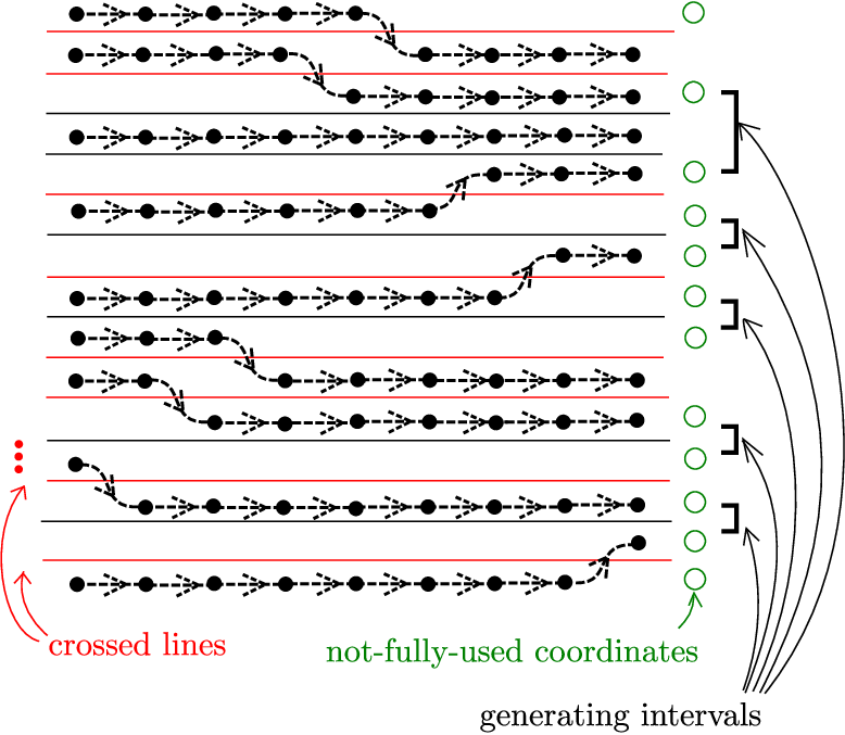
When working with algebras (like ℬ0​(n,k)\mathcal{B}_{0}(n,k) and ℬ⁡(n,k,𝒮)\mathcal{B}(n,k,\mathcal{S})) that come with a distinguished collection of idempotents, we freely make use of the perspective of differential graded categories. For the reader’s convenience, a review of the relevant category theory is included in Appendix A. In Section 4, we use Ozsváth–Szabó’s notion of “generating intervals” to give a decomposition theorem (Corollary 4.16) for Hom-spaces in the category associated to ℬ⁡(n,k,𝒮)\mathcal{B}(n,k,\mathcal{S}). In Section 5 we use this decomposition theorem to compute the homology of ℬ⁡(n,k,𝒮)\mathcal{B}(n,k,\mathcal{S}), proving Theorem 1.3. We also investigate formality in Section 5, proving Theorem 1.4 and its analogues for the truncated algebras.

Acknowledgments

The authors would like to thank Francis Bonahon, Ko Honda, Aaron Lauda, Robert Lipshitz, Ciprian Manolescu, Peter Ozsváth, Raphaël Rouquier, and Zoltán Szabó for many useful conversations. The first named author would especially like to thank Zoltán Szabó for teaching him about the Kauffman-states functor.

2. Quiver descriptions of Ozsváth-Szabó’s algebra ℬ0\mathcal{B}_{0}

2.1. Quiver algebras

Definition 2.1.

Let Γ\Gamma be a finite directed graph, allowed to have loops and multi-edges, and let VV and EE denote the sets of vertices and edges (or arrows) of Γ\Gamma respectively. A path γ\gamma in Γ\Gamma is given by a finite sequence of edges, written γ=(γ1,…,γl)\gamma=(\gamma_{1},\ldots,\gamma_{l}) (when l=1l=1 we omit the parentheses), such that for all i=1,…,l−1i=1,\ldots,l-1, the ending vertex of γi\gamma_{i} coincides with the starting vertex of γi+1\gamma_{i+1}. The start of a path γ=(γ1,…,γl)\gamma=(\gamma_{1},\ldots,\gamma_{l}) is the starting vertex of γ1\gamma_{1}, denoted by v1v_{1}. Likewise the end of γ\gamma is the ending vertex of γl\gamma_{l}, denoted by vl+1v_{l+1}. The number ll is called the length of γ\gamma.

For every vertex v∈Vv\in V, there is a distinguished path IvI_{v} from vv to vv of length 00, given by the empty sequence of edges.

Given a finite directed graph Γ\Gamma, one can construct the path algebra over Γ\Gamma with coefficients in a commutative ring 𝕜\Bbbk (in this paper, 𝕜\Bbbk will always be either the two element field 𝔽2\mathbb{F}_{2} or a polynomial ring over 𝔽2\mathbb{F}_{2}). The path IvI_{v} induces a (distinguished) idempotent in this algebra. In order to remember that this algebra comes with a set of distinguished idempotents, we can use the category defined below. For a review of some definitions concerning algebras and categories (e.g. 𝕜\Bbbk-linear category), see Appendix A. Note that for us a 𝕜\Bbbk-algebra is a ring 𝒜\mathcal{A} equipped with a ring homomorphism 𝕜→𝒜\Bbbk\to\mathcal{A}; see Remark A.1.

Definition 2.2.

Let Γ\Gamma be a finite directed graph as above and let 𝕜\Bbbk be a commutative ring. Define 𝕜​Γ\Bbbk\Gamma to be the 𝕜\Bbbk-linear category whose objects are vertices v∈Vv\in V of Γ\Gamma and such that for two vertices v1,v2∈Vv_{1},v_{2}\in V, Hom𝕜​Γ⁡(v2,v1)\Hom_{\Bbbk\Gamma}(v_{2},v_{1}) is the free 𝕜\Bbbk-module formally spanned by all paths in Γ\Gamma from v1v_{1} to v2v_{2}. Composition of morphisms in Γ\Gamma is given by concatenation of paths, extended linearly over 𝕜\Bbbk, and identity morphisms 𝐈v\mathbf{I}_{v} for v∈Vv\in V are given by the “empty” paths IvI_{v}.

Remark 2.3.

The reversal of directions in Definition 2.2 is intentional; one wants compositions f​gfg in a category, thought of as “ff after gg,” to agree with multiplications a​bab in a path algebra, thought of as “bb after aa” and determined by edges v1→𝑎v2→𝑏v3v_{1}\xrightarrow{a}v_{2}\xrightarrow{b}v_{3} in Γ\Gamma.

As defined in Section A.3, we have an 𝕀\mathbb{I}-algebra Alg𝕜​Γ\Alg_{\Bbbk\Gamma}, where 𝕀=𝕜V\mathbb{I}=\Bbbk^{V}. This algebra is called the path algebra of Γ\Gamma; we will denote it by Path⁡(Γ)\Path(\Gamma). When the coefficient ring 𝕜\Bbbk is not clear from the context, we will denote it by Path𝕜⁡(Γ)\Path_{\Bbbk}(\Gamma). The set {𝐈v|v∈V}\left\{\mathbf{I}_{v}\,\middle|\,v\in V\right\} is a set of pairwise orthogonal idempotents in Path⁡(Γ)\Path(\Gamma): for all vv, v′∈Vv^{\prime}\in V we have

𝐈v⋅𝐈v′={𝐈vif v=v′0otherwise.\mathbf{I}_{v}\cdot\mathbf{I}_{v^{\prime}}=\begin{cases}\mathbf{I}_{v}&\text{if $v=v^{\prime}$}\\ 0&\text{otherwise.}\end{cases}

The identity element of Path⁡(Γ)\Path(\Gamma) is ∑v∈V𝐈v\sum_{v\in V}\mathbf{I}_{v}.

The edges of Γ\Gamma give a natural set of multiplicative generators for Path⁡(Γ)\Path(\Gamma); paths in Γ\Gamma as defined in Definition 2.1 give a basis for Path⁡(Γ)\Path(\Gamma) as a free module over 𝕜\Bbbk.

More generally, as explained in detail in Appendix A, given a 𝕜\Bbbk-linear category 𝒞\mathcal{C} with (finite) object set VV, one can form a corresponding 𝕀\mathbb{I}-algebra Alg𝒞\Alg_{\mathcal{C}} by summing over the morphism spaces. The composition of the inclusion of constant functions 𝕜→𝕀\Bbbk\to\mathbb{I} with the ring homomorphism 𝕀→Alg𝒞\mathbb{I}\to\Alg_{\mathcal{C}} has image contained in the center of Alg𝒞\Alg_{\mathcal{C}}. Vice versa, given an 𝕀\mathbb{I}-algebra 𝒜\mathcal{A} such that the natural map 𝕜→𝕀→𝒜\Bbbk\to\mathbb{I}\to\mathcal{A} has image in Z⁡(𝒜)Z(\mathcal{A}), one can form a 𝕜\Bbbk-linear category Cat𝒜\Cat_{\mathcal{A}} with object set VV. Moreover, functors between 𝕜\Bbbk-linear categories that are the identity on objects correspond to 𝕀\mathbb{I}-algebra homomorphisms.

Remark 2.4.

We will often refer to certain functors as being equivalent to algebra homomorphisms; we assume without further mention that all functors discussed in this context are the identity on objects. Also, when discussing algebras 𝒜\mathcal{A} over 𝕀=𝕜V\mathbb{I}=\Bbbk^{V} for a finite set VV, we will assume that the natural map 𝕜→𝕀→𝒜\Bbbk\to\mathbb{I}\to\mathcal{A} has image in Z⁡(𝒜)Z(\mathcal{A}).

Definition 2.5.

Let Γ\Gamma be a directed graph with vertex set VV. For v,v′∈Vv,v^{\prime}\in V, let ℛv,v′\mathcal{R}_{v,v^{\prime}} be a subset of Hom𝕜​Γ⁡(v′,v)\Hom_{\Bbbk\Gamma}(v^{\prime},v). Let ℛ\mathcal{R} be the union of ℛv,v′\mathcal{R}_{v,v^{\prime}} over all v,v′∈Vv,v^{\prime}\in V, viewed as a subset of Path⁡(Γ)\Path(\Gamma); we will call ℛ\mathcal{R} a set of relations. Let 𝕀=𝕜V\mathbb{I}=\Bbbk^{V} as usual. We define the quiver algebra with relations Quiv⁡(Γ,ℛ)\Quiv(\Gamma,\mathcal{R}) to be the 𝕀\mathbb{I}-algebra

Quiv⁡(Γ,ℛ)=Path⁡(Γ)ℐℛ,\Quiv(\Gamma,\mathcal{R})=\frac{\Path(\Gamma)}{\mathcal{I}_{\mathcal{R}}},

where ℐℛ\mathcal{I}_{\mathcal{R}} is the two-sided ideal generated by the relation set ℛ\mathcal{R}. We have a corresponding category CatQuiv⁡(Γ,ℛ)\Cat_{\Quiv(\Gamma,\mathcal{R})} with object set VV.

The edges of Γ\Gamma still give a natural set of multiplicative generators for Quiv⁡(Γ,ℛ)\Quiv(\Gamma,\mathcal{R}). Paths in Γ\Gamma give a spanning set for Quiv⁡(Γ,ℛ)\Quiv(\Gamma,\mathcal{R}) over 𝕜\Bbbk; since we have imposed relations, the set of paths in Γ\Gamma might no longer be linearly independent. We will refer to elements of this spanning set as path-like elements or additive generators of Quiv⁡(Γ,ℛ)\Quiv(\Gamma,\mathcal{R}).

The following proposition is standard.

Proposition 2.6.

Let Γ\Gamma be a finite directed graph with vertex set VV and edge set EE. Let 𝒞\mathcal{C} be any 𝕜\Bbbk-linear category whose set of objects is VV. Suppose that for each edge γ∈E\gamma\in E starting at v1v_{1} and ending at v2v_{2}, we have a morphism F⁡(γ):v2→v1F(\gamma):v_{2}\to v_{1} in 𝒞\mathcal{C}. Then, there is a unique 𝕜\Bbbk-linear functor from 𝕜​Γ\Bbbk\Gamma to 𝒞\mathcal{C} sending vv to vv for all v∈Vv\in V and sending γ\gamma to F⁡(γ)F(\gamma) for all γ∈E\gamma\in E.

This functor gives us a homomorphism of 𝕀\mathbb{I}-algebras from Path⁡(Γ)\Path(\Gamma) to Alg𝒞\Alg_{\mathcal{C}}. If this homomorphism sends ℛ⊂Path⁡(Γ)\mathcal{R}\subset\Path(\Gamma) to zero, we get a homomorphism of 𝕀\mathbb{I}-algebras from Quiv⁡(Γ,ℛ)\Quiv(\Gamma,\mathcal{R}) to Alg𝒞\Alg_{\mathcal{C}}, or equivalently a functor from CatQuiv⁡(Γ,ℛ)\Cat_{\Quiv(\Gamma,\mathcal{R})} to 𝒞\mathcal{C}.

It will be convenient to have dg (i.e. differential graded) versions of the above constructions; the proofs of the below propositions are left to the reader. We discuss gradings first.

Proposition 2.7.

Let Γ\Gamma, VV, and ℛ\mathcal{R} be as in Definition 2.5, and let GG be a group. Suppose that for each edge γ\gamma of Γ\Gamma, we are given an element deg⁡(γ)∈G\deg(\gamma)\in G. Extend deg\deg multiplicatively to a map from paths in Γ\Gamma to GG. Assume that each relation r∈ℛr\in\mathcal{R} is a sum of paths with the same degree. Then deg\deg gives Quiv⁡(Γ,ℛ)\Quiv(\Gamma,\mathcal{R}) the structure of a GG-graded 𝕀\mathbb{I}-algebra (see Appendix A.1 for a brief review of our grading conventions).

Next we discuss the differential.

Proposition 2.8.

Let Γ\Gamma, VV, and ℛ\mathcal{R} be as in Definition 2.5. Suppose we are given an element ∂(γ)\partial(\gamma) of 𝐈𝐱​Path⁡(Γ)​𝐈𝐲\mathbf{I}_{\mathbf{x}}\Path(\Gamma)\mathbf{I}_{\mathbf{y}} for each edge γ\gamma of Γ\Gamma from a vertex 𝐱\mathbf{x} to another vertex 𝐲\mathbf{y}. Extend ∂\partial to Path⁡(Γ)\Path(\Gamma) linearly and using the Leibniz rule. Assume that ∂(ℛ)=0\partial(\mathcal{R})=0 and that ∂2(γ)=0\partial^{2}(\gamma)=0 for each edge γ\gamma. Then ∂\partial gives Quiv⁡(Γ,ℛ)\Quiv(\Gamma,\mathcal{R}) the structure of a differential 𝕀\mathbb{I}-algebra.

If Quiv⁡(Γ,ℛ)\Quiv(\Gamma,\mathcal{R}) has a GG-grading for some group GG, we have λ∈Z⁡(G)\lambda\in Z(G), and ∂\partial is homogeneous of degree λ−1\lambda^{-1}, then ∂\partial gives Quiv⁡(Γ,ℛ)\Quiv(\Gamma,\mathcal{R}) the structure of a (G,λ)(G,\lambda)-graded dg 𝕀\mathbb{I}-algebra. If the GG-grading on Quiv⁡(Γ,ℛ)\Quiv(\Gamma,\mathcal{R}) comes from Proposition 2.7, then ∂\partial is homogeneous of degree λ−1\lambda^{-1} as long as ∂(γ)\partial(\gamma) is homogeneous of degree λ−1​deg⁡(γ)\lambda^{-1}\deg(\gamma) for each edge γ\gamma of Γ\Gamma.

There are graded, differential, and dg analogues of Proposition 2.6.

2.2. The algebra ℬ0​(n,k)\mathcal{B}_{0}(n,k)

In this section we present two quiver descriptions for the algebra ℬ0​(n,k)\mathcal{B}_{0}(n,k) from [OSz18]. The first of these will be a direct translation of the definition in that paper. Proving that the second description is equivalent to the first will be the goal of Section 2.4.

2.2.1. I-states

Throughout the paper, let [0,n][0,n] denote the set {0,1,2,…,n}\{0,1,2,\ldots,n\}. Ozsváth–Szabó [OSz18, Section 3.1] define an I-state to be a subset 𝐱\mathbf{x} of [0,n][0,n] with |x|=k|x|=k. By convention, we write the elements of an I-state 𝐱\mathbf{x} in increasing order as 𝐱={x1,…,xk}\mathbf{x}=\{x_{1},\ldots,x_{k}\} with x1<⋯<xkx_{1}<\cdots<x_{k}. Let V⁡(n,k)V(n,k) be the set of I-states for a given nn and kk. The algebras ℬ0​(n,k)\mathcal{B}_{0}(n,k) and ℬ⁡(n,k)\mathcal{B}(n,k) can be viewed as algebras over 𝔽2V⁡(n,k)\mathbb{F}_{2}^{V(n,k)}; we will call 𝔽2V⁡(n,k)\mathbb{F}_{2}^{V(n,k)} the ring of idempotents and denote it by 𝐈⁡(n,k)\mathbf{I}(n,k).

Definition 2.9 ([OSz18, Section 3.1]).

Let 𝐱,𝐲∈V⁡(n,k)\mathbf{x},\mathbf{y}\in V(n,k). The minimal relative weight vector v⁡(𝐱,𝐲)=(v1​(𝐱,𝐲),…,vn​(𝐱,𝐲))∈ℤnv(\mathbf{x},\mathbf{y})=(v_{1}(\mathbf{x},\mathbf{y}),\ldots,v_{n}(\mathbf{x},\mathbf{y}))\in\mathbb{Z}^{n} is defined by the formula

vi​(𝐱,𝐲)=|𝐲∩[i,n]|−|𝐱∩[i,n]|.v_{i}(\mathbf{x},\mathbf{y})=|\mathbf{y}\cap[i,n]|-|\mathbf{x}\cap[i,n]|.

The minimal relative grading vector |v|​(𝐱,𝐲)|v|(\mathbf{x},\mathbf{y}) is defined by |v|i​(𝐱,𝐲)=|vi​(𝐱,𝐲)||v|_{i}(\mathbf{x},\mathbf{y})=|v_{i}(\mathbf{x},\mathbf{y})|.

It is straightforward to check that, for 𝐱,𝐲,𝐳∈V⁡(n,k)\mathbf{x},\mathbf{y},\mathbf{z}\in V(n,k), we have

(2.1) v⁡(𝐱,𝐳)=v⁡(𝐱,𝐲)+v⁡(𝐲,𝐳).v(\mathbf{x},\mathbf{z})=v(\mathbf{x},\mathbf{y})+v(\mathbf{y},\mathbf{z}).

The functions |v|i|v|_{i} are not additive in general, but they are subadditive.

Proposition 2.10 ([OSz18, Section 3.1]).

For 𝐱,𝐲,𝐳∈V⁡(n,k)\mathbf{x},\mathbf{y},\mathbf{z}\in V(n,k) and 1≤i≤n1\leq i\leq n, |v|i​(𝐲,𝐳)−|v|i​(𝐱,𝐳)+|​v|i​(𝐱,𝐲)|v|_{i}(\mathbf{y},\mathbf{z})-|v|_{i}(\mathbf{x},\mathbf{z})+|v|_{i}(\mathbf{x},\mathbf{y}) is a nonnegative even integer.

2.2.2. The algebras

We start with a simple rephrasing of Ozsváth–Szabó’s definition of ℬ0​(n,k)\mathcal{B}_{0}(n,k) (see [OSz18, Section 3.1]).

Definition 2.11.

Let K⁡(n,k)K(n,k) denote the complete directed graph with vertex set V=V⁡(n,k)V=V(n,k) (this graph has a unique edge from 𝐱\mathbf{x} to 𝐲\mathbf{y} for every ordered pair (𝐱,𝐲)∈V2(\mathbf{x},\mathbf{y})\in V^{2}). Denote the edge in K⁡(n,k)K(n,k) from 𝐱\mathbf{x} to 𝐲\mathbf{y} by f𝐱,𝐲f_{\mathbf{x},\mathbf{y}}. Write Path⁡(K⁡(n,k))\Path(K(n,k)) for Alg𝔽2​[U1,…,Un]​K​(n,k)\Alg_{\mathbb{F}_{2}[U_{1},\ldots,U_{n}]K(n,k)}. Let ℛK⊂Path⁡(K⁡(n,k))\mathcal{R}_{K}\subset\Path(K(n,k)) denote the set of elements

f𝐱,𝐲​f𝐲,𝐳−∏i=1nUi(|v|i​(𝐲,𝐳)−|v|i​(𝐱,𝐳)+|​v|i​(𝐱,𝐲))/2​f𝐱,𝐳f_{\mathbf{x},\mathbf{y}}f_{\mathbf{y},\mathbf{z}}-\prod_{i=1}^{n}U_{i}^{(|v|_{i}(\mathbf{y},\mathbf{z})-|v|_{i}(\mathbf{x},\mathbf{z})+|v|_{i}(\mathbf{x},\mathbf{y}))/2}f_{\mathbf{x},\mathbf{z}}

for all ordered triples (𝐱,𝐲,𝐳)∈V3(\mathbf{x},\mathbf{y},\mathbf{z})\in V^{3}. Define

ℬ0​(n,k):=Quiv⁡(K⁡(n,k),ℛK),\mathcal{B}_{0}(n,k):=\Quiv(K(n,k),\mathcal{R}_{K}),

an algebra over 𝔽2​[U1,…,Un]V⁡(n,k)\mathbb{F}_{2}[U_{1},\ldots,U_{n}]^{V(n,k)}; we have an 𝔽2​[U1,…,Un]\mathbb{F}_{2}[U_{1},\ldots,U_{n}]-linear category Catℬ0​(n,k)\Cat_{\mathcal{B}_{0}(n,k)} with set of objects V⁡(n,k)V(n,k). One can check that for 𝐱,𝐲∈V⁡(n,k)\mathbf{x},\mathbf{y}\in V(n,k), the 𝔽2​[U1,…,Un]\mathbb{F}_{2}[U_{1},\ldots,U_{n}]-linear map ϕ𝐱,𝐲\phi^{\mathbf{x},\mathbf{y}} from 𝔽2​[U1,…,Un]\mathbb{F}_{2}[U_{1},\ldots,U_{n}] to 𝐈𝐱​ℬ0​(n,k)​𝐈𝐲\mathbf{I}_{\mathbf{x}}\mathcal{B}_{0}(n,k)\mathbf{I}_{\mathbf{y}} sending 11 to f𝐱,𝐲f_{\mathbf{x},\mathbf{y}} is a bijection. Thus, Quiv⁡(K⁡(n,k),ℛK)\Quiv(K(n,k),\mathcal{R}_{K}) agrees with Ozsváth–Szabó’s definition of ℬ0​(n,k)\mathcal{B}_{0}(n,k).

We now give an alternate definition of ℬ0​(n,k)\mathcal{B}_{0}(n,k); we will prove below that the algebra Quiv⁡(Γ⁡(n,k),ℛ)\Quiv(\Gamma(n,k),\mathcal{R}) constructed in the following definition is isomorphic to ℬ0​(n,k)\mathcal{B}_{0}(n,k).

Definition 2.12.

The directed graph Γ⁡(n,k)\Gamma(n,k) has vertex set V=V⁡(n,k)V=V(n,k). Its arrows are given as follows:

  • •

    For vertices 𝐱\mathbf{x} with i−1∈𝐱i-1\in\mathbf{x} and i∉𝐱i\notin\mathbf{x}, there is an arrow from 𝐱\mathbf{x} to (𝐱∖{i−1})∪{i}(\mathbf{x}\setminus\left\{i-1\right\})\cup\left\{i\right\}, said to have label RiR_{i}.

  • •

    For vertices 𝐱\mathbf{x} with i∈𝐱i\in\mathbf{x} and i−1∉𝐱i-1\notin\mathbf{x}, there is an arrow from 𝐱\mathbf{x} to (𝐱∖{i})∪{i−1}(\mathbf{x}\setminus\left\{i\right\})\cup\left\{i-1\right\}, said to have label LiL_{i}.

  • •

    For all vertices 𝐱\mathbf{x} and all ii between 11 and nn, there is an arrow from 𝐱\mathbf{x} to 𝐱\mathbf{x}, said to have label UiU_{i}.

We write Path⁡(Γ⁡(n,k))\Path(\Gamma(n,k)) for Alg𝔽2​Γ​(n,k)\Alg_{\mathbb{F}_{2}\Gamma(n,k)}. To each basis element γ\gamma of Path⁡(Γ⁡(n,k))\Path(\Gamma(n,k)), we can associate a (non-commutative) monomial μ⁡(γ)\mu(\gamma) in the letters RiR_{i}, LiL_{i}, and UiU_{i} for 1≤i≤n1\leq i\leq n. Note that two paths γ,γ′\gamma,\gamma^{\prime} with the same monomial and starting at the same vertex are equal. We then extend μ\mu 𝔽2\mathbb{F}_{2}-linearly to each element of Path⁡(Γ⁡(n,k))\Path(\Gamma(n,k)). For every pair of vertices 𝐱\mathbf{x} and 𝐲\mathbf{y}, we define ℛ𝐱,𝐲⊂Hom⁡(𝐲,𝐱)⊂Path⁡(Γ⁡(n,k))\mathcal{R}_{\mathbf{x},\mathbf{y}}\subset\Hom(\mathbf{y},\mathbf{x})\subset\Path(\Gamma(n,k)) to be the set of elements γ∈Hom⁡(𝐲,𝐱)\gamma\in\Hom(\mathbf{y},\mathbf{x}) such that μ⁡(γ)\mu(\gamma) is equal to one of the following:

  1. (1)

    Ri​Uj−Uj​RiR_{i}U_{j}-U_{j}R_{i},    Li​Uj−Uj​LiL_{i}U_{j}-U_{j}L_{i}, or Ui​Uj−Uj​UiU_{i}U_{j}-U_{j}U_{i} (the “UU central relations”),

  2. (2)

    Ri​Li−UiR_{i}L_{i}-U_{i} or Li​Ri−UiL_{i}R_{i}-U_{i} (the “loop relations”),

  3. (3)

    Ri​Rj−Rj​RiR_{i}R_{j}-R_{j}R_{i},    Li​Lj−Lj​LiL_{i}L_{j}-L_{j}L_{i}, or Ri​Lj−Lj​RiR_{i}L_{j}-L_{j}R_{i} for |i−j|>1|i-j|>1 (the “distant commutation relations”).

The minus signs could equally well be plus signs, since we are working over 𝔽2\mathbb{F}_{2}. We have an 𝐈⁡(n,k)\mathbf{I}(n,k)-algebra Quiv⁡(Γ⁡(n,k),ℛ)\Quiv(\Gamma(n,k),\mathcal{R}), where ℛ=⋃𝐱,𝐲ℛ𝐱,𝐲\mathcal{R}=\bigcup_{\mathbf{x},\mathbf{y}}\mathcal{R}_{\mathbf{x},\mathbf{y}}, and an 𝔽2\mathbb{F}_{2}-linear category CatQuiv⁡(Γ⁡(n,k),ℛ)\Cat_{\Quiv(\Gamma(n,k),\mathcal{R})} with object set V⁡(n,k)V(n,k). Using the edges of Γ⁡(n,k)\Gamma(n,k) with label UiU_{i}, we can give Quiv⁡(Γ⁡(n,k),ℛ)\Quiv(\Gamma(n,k),\mathcal{R}) the structure of an algebra over 𝔽2​[U1,…,Un]V⁡(n,k)\mathbb{F}_{2}[U_{1},\ldots,U_{n}]^{V(n,k)}. The relations (1) imply that the natural map 𝔽2​[U1,…,Un]→𝔽2​[U1,…,Un]V⁡(n,k)→Quiv⁡(Γ⁡(n,k),ℛ)\mathbb{F}_{2}[U_{1},\ldots,U_{n}]\to\mathbb{F}_{2}[U_{1},\ldots,U_{n}]^{V(n,k)}\to\Quiv(\Gamma(n,k),\mathcal{R}) has image in the center of Quiv⁡(Γ⁡(n,k),ℛ)\Quiv(\Gamma(n,k),\mathcal{R}). Equivalently, we can view CatQuiv⁡(Γ⁡(n,k),ℛ)\Cat_{\Quiv(\Gamma(n,k),\mathcal{R})} as an 𝔽2​[U1,…,Un]\mathbb{F}_{2}[U_{1},\ldots,U_{n}]-linear category.

2.3. Graphical interpretations

Refer to caption
Figure 1. Elements 𝐱\mathbf{x} and 𝐲\mathbf{y} of V⁡(5,3)V(5,3) viewed as dots occupying regions.

In this section we will give graphical interpretations of the algebras Quiv⁡(K⁡(n,k),ℛK)\Quiv(K(n,k),\mathcal{R}_{K}) and Quiv⁡(Γ⁡(n,k),ℛ)\Quiv(\Gamma(n,k),\mathcal{R}). In both interpretations we follow [OSz18] and interpret an I-state 𝐱\mathbf{x} as a choice of “occupied” regions between nn lines, illustrated with dots as in Figure 1.

Remark 2.13.

Our graphical conventions can be obtained from those used in [OSz18, OSz17] by 90∘90^{\circ} rotation clockwise. We perform this rotation to match Lipshitz–Ozsváth–Thurston and Zarev’s conventions for strands pictures in bordered Floer homology; see [MMW19] where we construct a quasi-isomorphism from ℬ⁡(n,k,𝒮)\mathcal{B}(n,k,\mathcal{S}) to a generalized strands algebra.

2.3.1. Graphical interpretation of Quiv⁡(K⁡(n,k),ℛK)\Quiv(K(n,k),\mathcal{R}_{K})

Refer to caption
Figure 2. Graphical interpretation of Quiv⁡(K⁡(n,k),ℛK)\Quiv(K(n,k),\mathcal{R}_{K}), for n=5n=5 and k=3k=3. We have 𝐱={0,2,5}\mathbf{x}=\{0,2,5\}, 𝐲={2,3,4}\mathbf{y}=\{2,3,4\}, and 𝐳={0,4,5}\mathbf{z}=\{0,4,5\}.

We start with an interpretation of the algebra Quiv⁡(K⁡(n,k),ℛK)\Quiv(K(n,k),\mathcal{R}_{K}). The generator f𝐱,𝐲f_{\mathbf{x},\mathbf{y}} of K⁡(n,k)K(n,k) is interpreted as a motion “all at once” of the dots comprising 𝐱\mathbf{x} to the dots comprising 𝐲\mathbf{y}; see the top line of Figure 2. Multiplying f𝐱,𝐲f_{\mathbf{x},\mathbf{y}} with f𝐲,𝐳f_{\mathbf{y},\mathbf{z}} always gives f𝐱,𝐳f_{\mathbf{x},\mathbf{z}} times a monomial pp in the UiU_{i} variables which can be described graphically as follows. Draw the picture for f𝐱,𝐲f_{\mathbf{x},\mathbf{y}} on the left of the picture for f𝐲,𝐳f_{\mathbf{y},\mathbf{z}}. The power of UiU_{i} in pp equals the number of distinct bigons with one edge on line ii and the other edge on a motion of a dot in the concatenated picture. See Figure 2 for an illustration.

2.3.2. Graphical interpretation of Quiv⁡(Γ⁡(n,k),ℛ)\Quiv(\Gamma(n,k),\mathcal{R})

Refer to caption
Figure 3. Graphical interpretation of Quiv⁡(Γ⁡(n,k),ℛ)\Quiv(\Gamma(n,k),\mathcal{R}), for n=5n=5 and k=3k=3.

Now we give a graphical interpretation of the algebra Quiv⁡(Γ⁡(n,k),ℛ)\Quiv(\Gamma(n,k),\mathcal{R}); see Figure 3. A path in Γ⁡(n,k)\Gamma(n,k) from 𝐱\mathbf{x} to 𝐲\mathbf{y} is interpreted as a motion “one dot-step at a time” of the dots comprising 𝐱\mathbf{x} to the dots comprising 𝐲\mathbf{y}. An edge labeled RiR_{i} moves a dot downwards one step; an edge labeled LiL_{i} moves a dot upwards one step (we suggest the mnemonics “Lift” and “loweR”). An edge labeled UiU_{i} does not move the dots at all, but we record that a UiU_{i} edge has been traversed. The basic idempotent 𝐈𝐱\mathbf{I}_{\mathbf{x}} can be interpreted as a stationary motion of the dots from 𝐱\mathbf{x} to itself. See also [OSz18, Remark 3.1].

Refer to caption
Figure 4. Relations in ℛ\mathcal{R}, viewed as motions as in Figure 3.

Note that during the motion of dots represented by any path γ\gamma in Γ⁡(n,k)\Gamma(n,k), there are never two dots in the same region between lines at any moment in the motion. The relations ℛ⊂Path⁡(Γ)\mathcal{R}\subset\Path(\Gamma) can be described in terms of motions as follows (see Figure 4):

  1. (1)

    Each UiU_{i} loop commutes with all other moves (this is the meaning of the UU central relations),

  2. (2)

    A dot passing back and forth through the ithi^{\text{th}} line is equivalent to a UiU_{i} loop (this is the meaning of the loop relations),

  3. (3)

    If two dots can each be moved by one slot independently of each other, then the order in which they are moved does not matter and thus they can be viewed as moving at the same time (this is the meaning of the distant commutation relations).

The next lemma says that the relative weight vector v⁡(𝐱,𝐲)v(\mathbf{x},\mathbf{y}) counts (with sign) the number of dots passing through each line in any path γ\gamma from 𝐱\mathbf{x} to 𝐲\mathbf{y}.

Lemma 2.14.

Let 𝐱,𝐲∈V⁡(n,k)\mathbf{x},\mathbf{y}\in V(n,k). Given any path γ\gamma in Γ⁡(n,k)\Gamma(n,k) from 𝐱\mathbf{x} to 𝐲\mathbf{y}, we have

vi​(𝐱,𝐲)=ρi​(γ)−λi​(γ)v_{i}(\mathbf{x},\mathbf{y})=\rho_{i}(\gamma)-\lambda_{i}(\gamma)

where ρi​(γ)\rho_{i}(\gamma) (respectively λi​(γ)\lambda_{i}(\gamma)) counts the number of edges labeled RiR_{i} (respectively LiL_{i}) in the path γ\gamma.

Proof.

By additivity of the right hand side of the formula under concatenation of paths, and by equation (2.1), we can assume that the path γ\gamma consists of a single edge. The formula is true when this edge has label RjR_{j}, LjL_{j}, or UjU_{j} (for both j=ij=i and j≠ij\neq i), as one can easily check from Definition 2.12. ∎

For a path γ\gamma in Γ⁡(n,k)\Gamma(n,k), represented visually by a motion of dots occurring one dot at a time, let F⁡(γ)F(\gamma) denote the same motion with all dots moving simultaneously (we will define FF rigorously below). If 𝐱→γ1𝐲→γ2𝐳\mathbf{x}\xrightarrow{\gamma_{1}}\mathbf{y}\xrightarrow{\gamma_{2}}\mathbf{z} are minimal-length paths in Γ⁡(n,k)\Gamma(n,k), then Lemma 2.14 implies that the quantity (|v|i​(𝐲,𝐳)−|v|i​(𝐱,𝐳)+|​v|i​(𝐱,𝐲))/2(|v|_{i}(\mathbf{y},\mathbf{z})-|v|_{i}(\mathbf{x},\mathbf{z})+|v|_{i}(\mathbf{x},\mathbf{y}))/2 counts extraneous pairs Ri,LiR_{i},L_{i} in the concatenation γ1​γ2\gamma_{1}\gamma_{2} (which the relations declare should be equivalent to UiU_{i} loops). This quantity is also the exponent of UiU_{i} appearing in the relations of Definition 2.11 for ℬ0​(n,k)\mathcal{B}_{0}(n,k) when one computes the product F⁡(γ1)​F​(γ2)F(\gamma_{1})F(\gamma_{2}).

Thus it is visually plausible that the “forget-the-ordering” map FF should be an algebra homomorphism from Quiv⁡(Γ⁡(n,k),ℛK)\Quiv(\Gamma(n,k),\mathcal{R}_{K}) to ℬ0​(n,k)\mathcal{B}_{0}(n,k) (we will prove this fact in Proposition 2.17). To prove that FF is a surjection, we just need to exhibit a path from 𝐱\mathbf{x} to 𝐲\mathbf{y} in Γ⁡(n,k)\Gamma(n,k), for all 𝐱,𝐲∈V⁡(n,k)\mathbf{x},\mathbf{y}\in V(n,k), whose image under FF is the generator f𝐱,𝐲f_{\mathbf{x},\mathbf{y}} of ℬ0​(n,k)\mathcal{B}_{0}(n,k); the existence of such a path is visually clear.

We will prove that FF is injective by constructing an inverse function GG to FF. For each pair 𝐱,𝐲\mathbf{x},\mathbf{y} of elements of V⁡(n,k)V(n,k), we will need to pick an explicit path γ𝐱,𝐲\gamma_{\mathbf{x},\mathbf{y}} in the preimage F−1​(f𝐱,𝐲)F^{-1}(f_{\mathbf{x},\mathbf{y}}), and we will need to show that the function G⁡(f𝐱,𝐲):=γ𝐱,𝐲G(f_{\mathbf{x},\mathbf{y}}):=\gamma_{\mathbf{x},\mathbf{y}} respects the relations of Definition 2.11. These will be the main technical tasks required to prove that ℬ0​(n,k)\mathcal{B}_{0}(n,k) and Quiv⁡(Γ⁡(n,k),ℛ)\Quiv(\Gamma(n,k),\mathcal{R}) describe the same algebra, which is the goal of Section 2.4.

2.4. Equivalence of descriptions

2.4.1. An intermediate description

We want to show that ℬ0​(n,k)\mathcal{B}_{0}(n,k) and Quiv⁡(Γ⁡(n,k),ℛ)\Quiv(\Gamma(n,k),\mathcal{R}) are isomorphic as 𝔽2​[U1,…,Un]V⁡(n,k)\mathbb{F}_{2}[U_{1},\ldots,U_{n}]^{V(n,k)}-algebras. To do so, it is convenient to introduce a third description of the same algebra.

Definition 2.15.

Let ΓU​(n,k)\Gamma_{U}(n,k) be the directed graph Γ⁡(n,k)\Gamma(n,k) with all edges labeled UiU_{i} removed. Let ℛU⊂Path𝔽2​[U1,…,Un]⁡(ΓU​(n,k))\mathcal{R}_{U}\subset\Path_{\mathbb{F}_{2}[U_{1},\ldots,U_{n}]}(\Gamma_{U}(n,k)) be defined analogously to ℛ⊂Path𝔽2⁡(Γ⁡(n,k))\mathcal{R}\subset\Path_{\mathbb{F}_{2}}(\Gamma(n,k)) from Definition 2.12, without elements of type (1), and interpreting any instance of UiU_{i} in a loop relation as a coefficient in 𝔽2​[U1,…,Un]\mathbb{F}_{2}[U_{1},\ldots,U_{n}] rather than a label for an edge.

Recall the discussion after Definition 2.12 about viewing CatQuiv⁡(Γ⁡(n,k),ℛ)\Cat_{\Quiv(\Gamma(n,k),\mathcal{R})} as being linear over 𝔽2​[U1,…,Un]\mathbb{F}_{2}[U_{1},\ldots,U_{n}]. The following lemma essentially says that this viewpoint is equivalent to building the category using Quiv⁡(ΓU​(n,k),ℛU)\Quiv(\Gamma_{U}(n,k),\mathcal{R}_{U}) rather than Quiv⁡(Γ⁡(n,k),ℛ)\Quiv(\Gamma(n,k),\mathcal{R}).

Lemma 2.16.

We have an isomorphism of 𝔽2​[U1,…,Un]\mathbb{F}_{2}[U_{1},\ldots,U_{n}]-linear categories

CatQuiv⁡(Γ⁡(n,k),ℛ)→≅CatQuiv⁡(ΓU​(n,k),ℛU).\Cat_{\Quiv(\Gamma(n,k),\mathcal{R})}\xrightarrow{\cong}\Cat_{\Quiv(\Gamma_{U}(n,k),\mathcal{R}_{U})}.

Equivalently, we have an isomorphism of 𝔽2​[U1,…,Un]V⁡(n,k)\mathbb{F}_{2}[U_{1},\ldots,U_{n}]^{V(n,k)}-algebras

Quiv⁡(Γ⁡(n,k),ℛ)→≅Quiv⁡(ΓU​(n,k),ℛU).\Quiv(\Gamma(n,k),\mathcal{R})\xrightarrow{\cong}\Quiv(\Gamma_{U}(n,k),\mathcal{R}_{U}).
Proof.

By Proposition 2.6, we have an 𝔽2\mathbb{F}_{2}-linear functor

ζ:𝔽2​Γ​(n,k)→CatQuiv⁡(ΓU​(n,k),ℛU)\zeta:\mathbb{F}_{2}\Gamma(n,k)\to\Cat_{\Quiv(\Gamma_{U}(n,k),\mathcal{R}_{U})}

defined as the identity on objects and by sending any edge (from some vertex vv to itself) labeled by UiU_{i} to the corresponding empty path IvI_{v} in Quiv⁡(ΓU​(n,k),ℛU)\Quiv(\Gamma_{U}(n,k),\mathcal{R}_{U}) with coefficient UiU_{i}, which gives the morphism v⟶Uivv\stackrel{{\scriptstyle U_{i}}}{{\longrightarrow}}v in CatQuiv⁡(ΓU​(n,k),ℛU)\Cat_{\Quiv(\Gamma_{U}(n,k),\mathcal{R}_{U})}. The functor ζ\zeta is defined to be the identity on all other edges. Incorporating the relations, ζ\zeta induces an 𝔽2\mathbb{F}_{2}-linear functor

ζ~:CatQuiv⁡(Γ⁡(n,k),ℛ)→CatQuiv⁡(ΓU​(n,k),ℛU);\widetilde{\zeta}:\Cat_{\Quiv(\Gamma(n,k),\mathcal{R})}\to\Cat_{\Quiv(\Gamma_{U}(n,k),\mathcal{R}_{U})};

one can check that ζ~\widetilde{\zeta} is in fact 𝔽2​[U1,…,Un]\mathbb{F}_{2}[U_{1},\ldots,U_{n}]-linear when viewing CatQuiv⁡(Γ⁡(n,k),ℛ)\Cat_{\Quiv(\Gamma(n,k),\mathcal{R})} as an 𝔽2​[U1,…,Un]\mathbb{F}_{2}[U_{1},\ldots,U_{n}]-linear category as discussed after Definition 2.12.

Similarly, we can build an 𝔽2\mathbb{F}_{2}-linear functor

ξ:𝔽2​[U1,…,Un]​ΓU​(n,k)→CatQuiv⁡(Γ⁡(n,k),ℛ)\xi:\mathbb{F}_{2}[U_{1},\ldots,U_{n}]\Gamma_{U}(n,k)\to\Cat_{\Quiv(\Gamma(n,k),\mathcal{R})}

by sending all objects vv to themselves, and sending any morphism in 𝔽2​[U1,…,Un]​ΓU​(n,k)\mathbb{F}_{2}[U_{1},\ldots,U_{n}]\Gamma_{U}(n,k) (which is an 𝔽2​[U1,…,Un]\mathbb{F}_{2}[U_{1},\ldots,U_{n}]-linear combination of paths) to the corresponding morphism in CatQuiv⁡(Γ⁡(n,k),ℛ)\Cat_{\Quiv(\Gamma(n,k),\mathcal{R})}, except that coefficients UiU_{i} are reinterpreted as concatenation with an edge labeled UiU_{i}. Because the UiU_{i}-edges exist at every vertex and commute with all others in Quiv⁡(Γ⁡(n,k),ℛ)\Quiv(\Gamma(n,k),\mathcal{R}), this assignment is well-defined independently of the choice of ordering. Our functor ξ\xi induces an 𝔽2\mathbb{F}_{2}-linear functor

ξ~:CatQuiv⁡(ΓU​(n,k),ℛU)→CatQuiv⁡(Γ⁡(n,k),ℛ)\widetilde{\xi}:\Cat_{\Quiv(\Gamma_{U}(n,k),\mathcal{R}_{U})}\to\Cat_{\Quiv(\Gamma(n,k),\mathcal{R})}

and again one can check that ξ~\widetilde{\xi} is 𝔽2​[U1,…,Un]\mathbb{F}_{2}[U_{1},\ldots,U_{n}]-linear when viewing CatQuiv⁡(Γ⁡(n,k),ℛ)\Cat_{\Quiv(\Gamma(n,k),\mathcal{R})} as an 𝔽2​[U1,…,Un]\mathbb{F}_{2}[U_{1},\ldots,U_{n}]-linear category.

By construction, ζ~\widetilde{\zeta} and ξ~\widetilde{\xi} are inverse isomorphisms of 𝔽2​[U1,…,Un]\mathbb{F}_{2}[U_{1},\ldots,U_{n}]-linear categories between CatQuiv⁡(Γ⁡(n,k),ℛ)\Cat_{\Quiv(\Gamma(n,k),\mathcal{R})} and CatQuiv⁡(ΓU​(n,k),ℛU)\Cat_{\Quiv(\Gamma_{U}(n,k),\mathcal{R}_{U})}, proving the claim. ∎

Thus, it suffices to show that ℬ0​(n,k)\mathcal{B}_{0}(n,k) and Quiv⁡(ΓU​(n,k),ℛU)\Quiv(\Gamma_{U}(n,k),\mathcal{R}_{U}) are isomorphic as algebras over 𝔽2​[U1,…,Un]V⁡(n,k)\mathbb{F}_{2}[U_{1},\ldots,U_{n}]^{V(n,k)}.

2.4.2. Constructing the forward homomorphism

Let 𝐱,𝐲∈V⁡(n,k)\mathbf{x},\mathbf{y}\in V(n,k). For any edge ee of ΓU​(n,k)\Gamma_{U}(n,k) from 𝐱\mathbf{x} to 𝐲\mathbf{y}, define F⁡(e)=f𝐱,𝐲∈HomCatℬ0​(n,k)⁡(𝐲,𝐱)F(e)=f_{\mathbf{x},\mathbf{y}}\in\Hom_{\Cat_{\mathcal{B}_{0}(n,k)}}(\mathbf{y},\mathbf{x}). By Proposition 2.6, FF extends uniquely to an 𝔽2​[U1,…,Un]\mathbb{F}_{2}[U_{1},\ldots,U_{n}]-linear functor from 𝔽2​[U1,…,Un]​ΓU​(n,k)\mathbb{F}_{2}[U_{1},\ldots,U_{n}]\Gamma_{U}(n,k) to Catℬ0​(n,k)\Cat_{\mathcal{B}_{0}(n,k)}, or equivalently a homomorphism of 𝔽2​[U1,…,Un]V⁡(n,k)\mathbb{F}_{2}[U_{1},\ldots,U_{n}]^{V(n,k)}-algebras from Path⁡(ΓU​(n,k))\Path(\Gamma_{U}(n,k)) to ℬ0​(n,k)\mathcal{B}_{0}(n,k).

Proposition 2.17.

The homomorphism of 𝔽2​[U1,…,Un]V⁡(n,k)\mathbb{F}_{2}[U_{1},\ldots,U_{n}]^{V(n,k)}-algebras

F:Path⁡(ΓU​(n,k))→ℬ0​(n,k)F:\Path(\Gamma_{U}(n,k))\to\mathcal{B}_{0}(n,k)

sends each element of ℛU⊂Path⁡(ΓU​(n,k))\mathcal{R}_{U}\subset\Path(\Gamma_{U}(n,k)) to zero.

Proof.

First, consider an element of ℛU\mathcal{R}_{U} of the form (γ1,γ2)−Ui​I𝐱(\gamma_{1},\gamma_{2})-U_{i}I_{\mathbf{x}}, where γ1\gamma_{1} is an edge from 𝐱\mathbf{x} to 𝐲\mathbf{y} with label RiR_{i} and γ2\gamma_{2} is an edge from 𝐲\mathbf{y} to 𝐱\mathbf{x} with label LiL_{i}. By Lemma 2.14, we have |v|i​(𝐱,𝐲)=|v|i​(𝐲,𝐱)=1|v|_{i}(\mathbf{x},\mathbf{y})=|v|_{i}(\mathbf{y},\mathbf{x})=1 and |v|j​(𝐱,𝐲)=|v|j​(𝐲,𝐱)=0|v|_{j}(\mathbf{x},\mathbf{y})=|v|_{j}(\mathbf{y},\mathbf{x})=0 for j≠ij\neq i. Since |vj|​(𝐱,𝐱)=0|v_{j}|(\mathbf{x},\mathbf{x})=0 for all jj, we have

F⁡(γ1)​F​(γ2)=f𝐱,𝐲​f𝐲,𝐱=Ui​f𝐱,𝐱=Ui​F​(I𝐱).F(\gamma_{1})F(\gamma_{2})=f_{\mathbf{x},\mathbf{y}}f_{\mathbf{y},\mathbf{x}}=U_{i}f_{\mathbf{x},\mathbf{x}}=U_{i}F(I_{\mathbf{x}}).

The argument for elements of ℛU\mathcal{R}_{U} of the form (γ1,γ2)−Ui​I𝐱(\gamma_{1},\gamma_{2})-U_{i}I_{\mathbf{x}} where γ1\gamma_{1} has label LiL_{i} and γ2\gamma_{2} has label RiR_{i} is similar.

Next, consider an element of ℛU\mathcal{R}_{U} of the form (γ1,γ2)−(γ3,γ4)(\gamma_{1},\gamma_{2})-(\gamma_{3},\gamma_{4}) where γ1\gamma_{1} is an edge from 𝐱\mathbf{x} to 𝐲\mathbf{y} with label RiR_{i}, γ2\gamma_{2} is an edge from 𝐲\mathbf{y} to 𝐳\mathbf{z} with label RjR_{j}, γ3\gamma_{3} is an edge from 𝐱\mathbf{x} to 𝐲′\mathbf{y}^{\prime} with label RjR_{j}, γ4\gamma_{4} is an edge from 𝐲′\mathbf{y}^{\prime} to 𝐳\mathbf{z} with label RiR_{i}, and |i−j|>1|i-j|>1. Again, by Lemma 2.14 we have

|v|i​(𝐱,𝐲)=|v|j​(𝐲,𝐳)=|v|i​(𝐱,𝐳)=|v|j​(𝐱,𝐳)=1.|v|_{i}(\mathbf{x},\mathbf{y})=|v|_{j}(\mathbf{y},\mathbf{z})=|v|_{i}(\mathbf{x},\mathbf{z})=|v|_{j}(\mathbf{x},\mathbf{z})=1.

By the same lemma we also have |v|j​(𝐱,𝐲)=|v|i​(𝐲,𝐳)=0|v|_{j}(\mathbf{x},\mathbf{y})=|v|_{i}(\mathbf{y},\mathbf{z})=0 as well as |v|l​(𝐱,𝐲)=|v|l​(𝐱,𝐳)=|v|l​(𝐲,𝐳)=0|v|_{l}(\mathbf{x},\mathbf{y})=|v|_{l}(\mathbf{x},\mathbf{z})=|v|_{l}(\mathbf{y},\mathbf{z})=0 for all l≠i,jl\neq i,j. It follows that

F⁡(γ1)​F​(γ2)=f𝐱,𝐲​f𝐲,𝐳=f𝐱,𝐳.F(\gamma_{1})F(\gamma_{2})=f_{\mathbf{x},\mathbf{y}}f_{\mathbf{y},\mathbf{z}}=f_{\mathbf{x},\mathbf{z}}.

A parallel argument shows that F⁡(γ3)​F​(γ4)=f𝐱,𝐳F(\gamma_{3})F(\gamma_{4})=f_{\mathbf{x},\mathbf{z}}, so we have F⁡(γ1)​F​(γ2)=F⁡(γ3)​F​(γ4)F(\gamma_{1})F(\gamma_{2})=F(\gamma_{3})F(\gamma_{4}). The rest of the cases are similar to this one. ∎

As a result we have a homomorphism of 𝔽2​[U1,…,Un]V⁡(n,k)\mathbb{F}_{2}[U_{1},\ldots,U_{n}]^{V(n,k)}-algebras

F:Quiv⁡(ΓU​(n,k),ℛU)→ℬ0​(n,k).F:\Quiv(\Gamma_{U}(n,k),\mathcal{R}_{U})\to\mathcal{B}_{0}(n,k).

2.4.3. Constructing the inverse homomorphism

In this section, we will define a homomorphism of 𝔽2​[U1,…,Un]V⁡(n,k)\mathbb{F}_{2}[U_{1},\ldots,U_{n}]^{V(n,k)}-algebras G:ℬ0​(n,k)→Quiv⁡(ΓU​(n,k),ℛU)G:\mathcal{B}_{0}(n,k)\to\Quiv(\Gamma_{U}(n,k),\mathcal{R}_{U}), or equivalently an 𝔽2​[U1,…,Un]\mathbb{F}_{2}[U_{1},\ldots,U_{n}]-linear functor from Catℬ0​(n,k)\Cat_{\mathcal{B}_{0}(n,k)} to CatQuiv⁡(ΓU​(n,k),ℛU)\Cat_{\Quiv(\Gamma_{U}(n,k),\mathcal{R}_{U})}.

We start by defining an 𝔽2​[U1,…,Un]\mathbb{F}_{2}[U_{1},\ldots,U_{n}]-linear functor

G:𝔽2​[U1,…,Un]​K​(n,k)→CatQuiv⁡(ΓU​(n,k),ℛU).G:\mathbb{F}_{2}[U_{1},\ldots,U_{n}]K(n,k)\to\Cat_{\Quiv(\Gamma_{U}(n,k),\mathcal{R}_{U})}.

By Proposition 2.6, it suffices to choose, for all pairs (𝐱,𝐲)∈V​(n,k)2(\mathbf{x},\mathbf{y})\in V(n,k)^{2}, a path γ𝐱,𝐲\gamma_{\mathbf{x},\mathbf{y}} in ΓU​(n,k)\Gamma_{U}(n,k) from 𝐱\mathbf{x} to 𝐲\mathbf{y}. We will further require that F⁡(γ𝐱,𝐲)=f𝐱,𝐲F(\gamma_{\mathbf{x},\mathbf{y}})=f_{\mathbf{x},\mathbf{y}}. We will choose γ𝐱,𝐲\gamma_{\mathbf{x},\mathbf{y}} recursively, but we need a few results first. The proof of the following lemma is left to the reader.

Lemma 2.18.

For 𝐱∈V⁡(n,k)\mathbf{x}\in V(n,k), suppose l∈𝐱l\in\mathbf{x} and l<m≤nl<m\leq n such that 𝐱∩[l,m]={l}\mathbf{x}\cap[l,m]=\{l\}. Let 𝐱′=(𝐱∖{l})∪{m}\mathbf{x}^{\prime}=(\mathbf{x}\setminus\{l\})\cup\{m\}. There exists a path γ\gamma from 𝐱\mathbf{x} to 𝐱′\mathbf{x}^{\prime} in ΓU​(n,k)\Gamma_{U}(n,k) whose edges are labeled Rl+1,…,RmR_{l+1},\ldots,R_{m} in order. The path γ\gamma is the unique path from 𝐱\mathbf{x} to 𝐱′\mathbf{x}^{\prime} with this property.

Lemma 2.19.

Under the assumptions of Lemma 2.18, let 𝐱=𝐱1,𝐱2,…,𝐱p=𝐱′\mathbf{x}=\mathbf{x}^{1},\mathbf{x}^{2},\ldots,\mathbf{x}^{p}=\mathbf{x}^{\prime} be the sequence of vertices traversed in the path γ\gamma of that lemma. We have f𝐱,𝐱′=f𝐱1,𝐱2⋯f𝐱p−1,𝐱pf_{\mathbf{x},\mathbf{x}^{\prime}}=f_{\mathbf{x}^{1},\mathbf{x}^{2}}\cdots f_{\mathbf{x}^{p-1},\mathbf{x}^{p}}.

Proof.

Induct on p≥2p\geq 2; the case p=2p=2 is tautological. Assume that

f𝐱1,𝐱p−1=f𝐱1,𝐱2,⋯,f𝐱p−2,𝐱p−1.f_{\mathbf{x}^{1},\mathbf{x}^{p-1}}=f_{\mathbf{x}^{1},\mathbf{x}^{2}},\cdots,f_{\mathbf{x}^{p-2},\mathbf{x}^{p-1}}.

It suffices to show that f𝐱1,𝐱p=f𝐱1,𝐱p−1​f𝐱p−1,𝐱pf_{\mathbf{x}^{1},\mathbf{x}^{p}}=f_{\mathbf{x}^{1},\mathbf{x}^{p-1}}f_{\mathbf{x}^{p-1},\mathbf{x}^{p}}. For l+1≤i≤m−1l+1\leq i\leq m-1, we have |v|i​(𝐱1,𝐱p)=1|v|_{i}(\mathbf{x}^{1},\mathbf{x}^{p})=1, |v|i​(𝐱1,𝐱p−1)=1|v|_{i}(\mathbf{x}^{1},\mathbf{x}^{p-1})=1, and |v|i​(𝐱p−1,𝐱p)=0|v|_{i}(\mathbf{x}^{p-1},\mathbf{x}^{p})=0 by Lemma 2.14. For i=mi=m, we have |v|i​(𝐱1,𝐱p)=1|v|_{i}(\mathbf{x}^{1},\mathbf{x}^{p})=1, |v|i​(𝐱1,𝐱p−1)=0|v|_{i}(\mathbf{x}^{1},\mathbf{x}^{p-1})=0, and |v|i​(𝐱p−1,𝐱p)=1|v|_{i}(\mathbf{x}^{p-1},\mathbf{x}^{p})=1. For i∉[l+1,m]i\notin[l+1,m], we have |v|i​(𝐱1,𝐱p)=|v|i​(𝐱1,𝐱p−1)=|v|i​(𝐱p−1,𝐱p)=0|v|_{i}(\mathbf{x}^{1},\mathbf{x}^{p})=|v|_{i}(\mathbf{x}^{1},\mathbf{x}^{p-1})=|v|_{i}(\mathbf{x}^{p-1},\mathbf{x}^{p})=0. Thus, the lemma follows from the relations defining multiplication in ℬ0​(n,k)\mathcal{B}_{0}(n,k). ∎

Corollary 2.20.

Under the assumptions of Lemma 2.18, we have F⁡(γ)=f𝐱,𝐱′F(\gamma)=f_{\mathbf{x},\mathbf{x}^{\prime}}, where γ\gamma is the path constructed in that lemma and FF was defined in Section 2.4.2.

Proof.

Write γ=(γl+1,…,γm)\gamma=(\gamma_{l+1},\ldots,\gamma_{m}) where γi\gamma_{i} has label RiR_{i}. We have F(γ)=F(γl+1)⋯F(γm)=f𝐱1,𝐱2⋯f𝐱p−1,𝐱pF(\gamma)=F(\gamma_{l+1})\cdots F(\gamma_{m})=f_{\mathbf{x}^{1},\mathbf{x}^{2}}\cdots f_{\mathbf{x}^{p-1},\mathbf{x}^{p}}, which equals f𝐱,𝐱′f_{\mathbf{x},\mathbf{x}^{\prime}} by Lemma 2.19. ∎

Lemma 2.21.

Let 𝐱,𝐲∈V⁡(n,k)\mathbf{x},\mathbf{y}\in V(n,k) with xa<yax_{a}<y_{a} for some a∈[1,k]a\in[1,k]; let aa be the maximal such index. We have 𝐱∩[xa,ya]={xa}\mathbf{x}\cap[x_{a},y_{a}]=\{x_{a}\}.

Proof.

Suppose xb∈𝐱x_{b}\in\mathbf{x} satisfies xa<xb≤yax_{a}<x_{b}\leq y_{a}. We have a<ba<b, so ya<yby_{a}<y_{b}. Thus, xb≤ya<ybx_{b}\leq y_{a}<y_{b}, contradicting the maximality of aa. ∎

Corollary 2.22.

Under the assumptions of Lemma 2.21, let 𝐱′=(𝐱∖{xa})∪{ya}\mathbf{x}^{\prime}=(\mathbf{x}\setminus\{x_{a}\})\cup\{y_{a}\}. We have f𝐱,𝐲=f𝐱,𝐱′​f𝐱′,𝐲f_{\mathbf{x},\mathbf{y}}=f_{\mathbf{x},\mathbf{x}^{\prime}}f_{\mathbf{x}^{\prime},\mathbf{y}}.

Proof.

For 1≤i≤n1\leq i\leq n, we want to show that |v|i​(𝐱,𝐲)=|v|i​(𝐱,𝐱′)+|​v|i​(𝐱′,𝐲)|v|_{i}(\mathbf{x},\mathbf{y})=|v|_{i}(\mathbf{x},\mathbf{x}^{\prime})+|v|_{i}(\mathbf{x}^{\prime},\mathbf{y}). First, note that if i∉[xa+1,ya]i\notin[x_{a}+1,y_{a}], then |𝐱′∩[i,n]|=|𝐱∩[i,n]||\mathbf{x}^{\prime}\cap[i,n]|=|\mathbf{x}\cap[i,n]| so that vi​(𝐱,𝐱′)=0v_{i}(\mathbf{x},\mathbf{x}^{\prime})=0 and

|vi|​(𝐱,𝐲)=||𝐲∩[i,n]|−|𝐱∩[i,n]||=||𝐲∩[i,n]|−|𝐱′∩[i,n]||=|vi|​(𝐱′,𝐲)+0|v_{i}|(\mathbf{x},\mathbf{y})=\Big||\mathbf{y}\cap[i,n]|-|\mathbf{x}\cap[i,n]|\Big|=\Big||\mathbf{y}\cap[i,n]|-|\mathbf{x}^{\prime}\cap[i,n]|\Big|=|v_{i}|(\mathbf{x}^{\prime},\mathbf{y})+0

as desired. Meanwhile, if i∈[xa+1,ya]i\in[x_{a}+1,y_{a}], we must have vi​(𝐱,𝐱′)=1v_{i}(\mathbf{x},\mathbf{x}^{\prime})=1. Furthermore, Lemma 2.21 ensures that xa′=yax_{a}^{\prime}=y_{a} is the smallest element of 𝐱′\mathbf{x}^{\prime} that is greater than or equal to ii, which in turn forces vi​(𝐱′,𝐲)≥0v_{i}(\mathbf{x}^{\prime},\mathbf{y})\geq 0. Thus the additivity of viv_{i} shows that vi​(𝐱,𝐲)≥0v_{i}(\mathbf{x},\mathbf{y})\geq 0 as well, and then the desired equality is immediate from the additivity of viv_{i}. ∎

There are also “upward-moving” versions of the above results involving edges labeled LiL_{i} rather than RiR_{i}.

Lemma 2.23.

For 𝐱∈V⁡(n,k)\mathbf{x}\in V(n,k), suppose l∈𝐱l\in\mathbf{x} and 0≤m<l0\leq m<l such that 𝐱∩[m,l]={l}\mathbf{x}\cap[m,l]=\{l\}. Let 𝐱′=(𝐱∖{l})∪{m}\mathbf{x}^{\prime}=(\mathbf{x}\setminus\{l\})\cup\{m\}. There exists a path γ\gamma from 𝐱\mathbf{x} to 𝐱′\mathbf{x}^{\prime} in ΓU​(n,k)\Gamma_{U}(n,k) whose edges are labeled Ll,…,Lm+1L_{l},\ldots,L_{m+1} in order. The path γ\gamma is the unique path from 𝐱\mathbf{x} to 𝐱′\mathbf{x}^{\prime} with this property.

Lemma 2.24.

Under the assumptions of Lemma 2.23, let 𝐱=𝐱1,𝐱2,…,𝐱p=𝐱′\mathbf{x}=\mathbf{x}^{1},\mathbf{x}^{2},\ldots,\mathbf{x}^{p}=\mathbf{x}^{\prime} be the sequence of vertices traversed in the path γ\gamma of that lemma. We have f𝐱,𝐱′=f𝐱1,𝐱2⋯f𝐱p−1,𝐱pf_{\mathbf{x},\mathbf{x}^{\prime}}=f_{\mathbf{x}^{1},\mathbf{x}^{2}}\cdots f_{\mathbf{x}^{p-1},\mathbf{x}^{p}}.

Corollary 2.25.

Under the assumptions of Lemma 2.23, we have F⁡(γ)=f𝐱,𝐱′F(\gamma)=f_{\mathbf{x},\mathbf{x}^{\prime}}, where γ\gamma is the path constructed in that lemma.

Lemma 2.26.

Let 𝐱,𝐲∈V⁡(n,k)\mathbf{x},\mathbf{y}\in V(n,k) with xa>yax_{a}>y_{a} for some a∈[1,k]a\in[1,k]; let aa be the minimal such index. We have 𝐱∩[ya,xa]={xa}\mathbf{x}\cap[y_{a},x_{a}]=\{x_{a}\}.

Corollary 2.27.

Under the assumptions of Lemma 2.26, let 𝐱′=(𝐱∖{xa})∪{ya}\mathbf{x}^{\prime}=(\mathbf{x}\setminus\{x_{a}\})\cup\{y_{a}\}. We have f𝐱,𝐲=f𝐱,𝐱′​f𝐱′,𝐲f_{\mathbf{x},\mathbf{y}}=f_{\mathbf{x},\mathbf{x}^{\prime}}f_{\mathbf{x}^{\prime},\mathbf{y}}.

Now we recursively define a path γ𝐱,𝐲\gamma_{\mathbf{x},\mathbf{y}} in ΓU​(n,k)\Gamma_{U}(n,k) from 𝐱\mathbf{x} to 𝐲\mathbf{y}.

Definition 2.28.

Our recursion scheme will involve the quantity k−|𝐱∩𝐲|k-|\mathbf{x}\cap\mathbf{y}|. If this quantity is zero, then 𝐱=𝐲\mathbf{x}=\mathbf{y}. Define γ𝐱,𝐱=I𝐱\gamma_{\mathbf{x},\mathbf{x}}=I_{\mathbf{x}}, the identity path at 𝐱\mathbf{x}. Since FF sends identity morphisms to identity morphisms, we have F⁡(γ𝐱,𝐱)=f𝐱,𝐱F(\gamma_{\mathbf{x},\mathbf{x}})=f_{\mathbf{x},\mathbf{x}}.

Now suppose we have 𝐱\mathbf{x} and 𝐲\mathbf{y}, and that we have constructed γ𝐱′,𝐲′\gamma_{\mathbf{x}^{\prime},\mathbf{y}^{\prime}} such that F⁡(γ𝐱′,𝐲′)=f𝐱′,𝐲′F(\gamma_{\mathbf{x}^{\prime},\mathbf{y}^{\prime}})=f_{\mathbf{x}^{\prime},\mathbf{y}^{\prime}} for all (𝐱′,𝐲′)(\mathbf{x}^{\prime},\mathbf{y}^{\prime}) with k−|𝐱′∩𝐲′|<k−|𝐱∩𝐲|k-|\mathbf{x}^{\prime}\cap\mathbf{y}^{\prime}|<k-|\mathbf{x}\cap\mathbf{y}|. To define γ𝐱,𝐲\gamma_{\mathbf{x},\mathbf{y}}, first suppose that xa<yax_{a}<y_{a} for some a∈[1,k]a\in[1,k]. Let aa be the maximal such index. By Lemma 2.21, we have 𝐱∩[xa,ya]={xa}\mathbf{x}\cap[x_{a},y_{a}]=\{x_{a}\}. Let 𝐱′=(𝐱∖{xa})∪{ya}\mathbf{x}^{\prime}=(\mathbf{x}\setminus\{x_{a}\})\cup\{y_{a}\}. By Lemma 2.18, there exists a unique path γ\gamma in ΓU​(n,k)\Gamma_{U}(n,k) from 𝐱\mathbf{x} to 𝐱′\mathbf{x}^{\prime} with edges labeled Rxa+1,…,RyaR_{x_{a}+1},\ldots,R_{y_{a}} in order, and we have F⁡(γ)=f𝐱,𝐱′F(\gamma)=f_{\mathbf{x},\mathbf{x}^{\prime}} by Corollary 2.20. Since k−|𝐱′∩𝐲|<k−|𝐱∩𝐲|k-|\mathbf{x}^{\prime}\cap\mathbf{y}|<k-|\mathbf{x}\cap\mathbf{y}|, we have already constructed a path γ𝐱′,𝐲\gamma_{\mathbf{x}^{\prime},\mathbf{y}} from 𝐱′\mathbf{x}^{\prime} to 𝐲\mathbf{y} with F⁡(γ𝐱′,𝐲)=f𝐱′,𝐲F(\gamma_{\mathbf{x}^{\prime},\mathbf{y}})=f_{\mathbf{x}^{\prime},\mathbf{y}}. Define

γ𝐱,𝐲:=γ⋅γ𝐱′,𝐲.\gamma_{\mathbf{x},\mathbf{y}}:=\gamma\cdot\gamma_{\mathbf{x}^{\prime},\mathbf{y}}.

We have F⁡(γ𝐱,𝐲)=F⁡(γ)​F​(γ𝐱′,𝐲)=f𝐱,𝐱′​f𝐱′,𝐲F(\gamma_{\mathbf{x},\mathbf{y}})=F(\gamma)F(\gamma_{\mathbf{x}^{\prime},\mathbf{y}})=f_{\mathbf{x},\mathbf{x}^{\prime}}f_{\mathbf{x}^{\prime},\mathbf{y}}, which equals f𝐱,𝐲f_{\mathbf{x},\mathbf{y}} by Corollary 2.22.

If xa≥yax_{a}\geq y_{a} for all aa but 𝐱≠𝐲\mathbf{x}\neq\mathbf{y}, let aa be the minimal index such that xa>yax_{a}>y_{a}. By Lemma 2.26, we have 𝐱∩[ya,xa]={xa}\mathbf{x}\cap[y_{a},x_{a}]=\{x_{a}\}. By Lemma 2.23, there exists a unique path γ\gamma from 𝐱\mathbf{x} to 𝐱′\mathbf{x}^{\prime} with edges labeled Lxa,…,Lya+1L_{x_{a}},\ldots,L_{y_{a}+1} in order, and we have F⁡(γ)=f𝐱,𝐱′F(\gamma)=f_{\mathbf{x},\mathbf{x}^{\prime}} by Corollary 2.25. As before, we have already constructed a path γ𝐱′,𝐲\gamma_{\mathbf{x}^{\prime},\mathbf{y}} from 𝐱′\mathbf{x}^{\prime} to 𝐲\mathbf{y} with F⁡(γ𝐱′,𝐲)=f𝐱′,𝐲F(\gamma_{\mathbf{x}^{\prime},\mathbf{y}})=f_{\mathbf{x}^{\prime},\mathbf{y}}. Define

γ𝐱,𝐲:=γ⋅γ𝐱′,𝐲.\gamma_{\mathbf{x},\mathbf{y}}:=\gamma\cdot\gamma_{\mathbf{x}^{\prime},\mathbf{y}}.

We have F⁡(γ𝐱,𝐲)=F⁡(γ)​F​(γ𝐱′,𝐲)=f𝐱,𝐱′​f𝐱′,𝐲F(\gamma_{\mathbf{x},\mathbf{y}})=F(\gamma)F(\gamma_{\mathbf{x}^{\prime},\mathbf{y}})=f_{\mathbf{x},\mathbf{x}^{\prime}}f_{\mathbf{x}^{\prime},\mathbf{y}} which equals f𝐱,𝐲f_{\mathbf{x},\mathbf{y}} by Corollary 2.27.

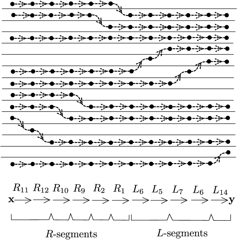
Refer to caption
Figure 5. The path γ𝐱,𝐲\gamma_{\mathbf{x},\mathbf{y}} in Example 2.29.
Example 2.29.

Let n=14n=14 and k=9k=9. For the elements 𝐱={0,1,3,6,7,8,9,10,14}\mathbf{x}=\{0,1,3,6,7,8,9,10,14\} and 𝐲={1,2,3,4,5,9,10,12,13}\mathbf{y}=\{1,2,3,4,5,9,10,12,13\} of V⁡(n,k)V(n,k), the path γ𝐱,𝐲\gamma_{\mathbf{x},\mathbf{y}} is shown in Figure 5 in the graphical notation of Section 2.3. Visually speaking, downward motions of dots happen first in γ𝐱,𝐲\gamma_{\mathbf{x},\mathbf{y}}, one dot at a time from bottom to top, and then upward motions of dots happen one dot at a time from top to bottom.

Definition 2.30.

Let

G:𝔽2​[U1,…,Un]​K​(n,k)→CatQuiv⁡(ΓU​(n,k),ℛU)G:\mathbb{F}_{2}[U_{1},\ldots,U_{n}]K(n,k)\to\Cat_{\Quiv(\Gamma_{U}(n,k),\mathcal{R}_{U})}

be the unique 𝔽2​[U1,…,Un]\mathbb{F}_{2}[U_{1},\ldots,U_{n}]-linear functor that is the identity on objects and such that G⁡(f𝐱,𝐲)G(f_{\mathbf{x},\mathbf{y}}) is the morphism in CatQuiv⁡(ΓU​(n,k),ℛU)\Cat_{\Quiv(\Gamma_{U}(n,k),\mathcal{R}_{U})} represented by γ𝐱,𝐲\gamma_{\mathbf{x},\mathbf{y}} for all edges f𝐱,𝐲f_{\mathbf{x},\mathbf{y}} in K⁡(n,k)K(n,k). We have a corresponding homomorphism

G:Path⁡(K⁡(n,k))→Quiv⁡(ΓU​(n,k),ℛU)G:\Path(K(n,k))\to\Quiv(\Gamma_{U}(n,k),\mathcal{R}_{U})

of 𝔽2​[U1,…,Un]V⁡(n,k)\mathbb{F}_{2}[U_{1},\ldots,U_{n}]^{V(n,k)}-algebras.

2.4.4. Proving that the inverse homomorphism is well-defined

In this section, we will show that the homomorphism GG of Definition 2.30 descends to a homomorphism G:ℬ0​(n,k)→Quiv⁡(ΓU​(n,k),ℛU)G:\mathcal{B}_{0}(n,k)\to\Quiv(\Gamma_{U}(n,k),\mathcal{R}_{U}); in Section 2.4.5 below, we will show that GG is the inverse of F:Quiv⁡(ΓU​(n,k),ℛU)→ℬ0​(n,k)F:\Quiv(\Gamma_{U}(n,k),\mathcal{R}_{U})\to\mathcal{B}_{0}(n,k). We start with some definitions and basic lemmas.

Definition 2.31.

If 𝐱,𝐲∈V⁡(n,k)\mathbf{x},\mathbf{y}\in V(n,k) with xa<yax_{a}<y_{a} for some a∈[1,k]a\in[1,k] and xb=ybx_{b}=y_{b} for all b≠ab\neq a, we will call γ𝐱,𝐲\gamma_{\mathbf{x},\mathbf{y}} an RR-segment. We define LL-segments similarly.

We note the following consequences of Definitions 2.28 and 2.31.

Corollary 2.32.

If γ𝐱,𝐲\gamma_{\mathbf{x},\mathbf{y}} is an RR-segment or an LL-segment, then γ𝐱,𝐲\gamma_{\mathbf{x},\mathbf{y}} is the path constructed in Lemma 2.18 or 2.23 respectively.

Corollary 2.33.

For any 𝐱,𝐲∈V⁡(n,k)\mathbf{x},\mathbf{y}\in V(n,k), either γ𝐱,𝐲\gamma_{\mathbf{x},\mathbf{y}} is trivial or we can write γ𝐱,𝐲=γ𝐱,𝐱′​γ𝐱′,𝐲\gamma_{\mathbf{x},\mathbf{y}}=\gamma_{\mathbf{x},\mathbf{x}^{\prime}}\gamma_{\mathbf{x}^{\prime},\mathbf{y}} where:

  1. (1)

    γ𝐱,𝐱′\gamma_{\mathbf{x},\mathbf{x}^{\prime}} is an RR-segment or an LL-segment;

  2. (2)

    |𝐱′∩𝐲|>|𝐱∩𝐲||\mathbf{x}^{\prime}\cap\mathbf{y}|>|\mathbf{x}\cap\mathbf{y}|;

  3. (3)

    if γ𝐱,𝐱′\gamma_{\mathbf{x},\mathbf{x}^{\prime}} is an RR-segment then ya=xa′y_{a}=x^{\prime}_{a} for the index aa with xa<xa′x_{a}<x^{\prime}_{a}, and yb≤xb′y_{b}\leq x^{\prime}_{b} for all b>ab>a;

  4. (4)

    if γ𝐱,𝐱′\gamma_{\mathbf{x},\mathbf{x}^{\prime}} is an LL-segment then ya=xa′y_{a}=x^{\prime}_{a} for the index aa with xa′<xax^{\prime}_{a}<x_{a}, yb≤xb′y_{b}\leq x^{\prime}_{b} for all bb, and yb=xb′y_{b}=x^{\prime}_{b} for all b<ab<a.

Refer to caption
Figure 6. Products of two RR-segments in Lemma 2.34: first two cases.
Refer to caption
Figure 7. Products of two RR-segments in Lemma 2.34: final case.
Refer to caption
Figure 8. Products of an RR-segment and an LL-segment in Lemma 2.34.
Refer to caption
Figure 9. Products of an LL-segment and an RR-segment in Lemma 2.34: one case.
Lemma 2.34.

If γ𝐱,𝐱′\gamma_{\mathbf{x},\mathbf{x}^{\prime}} and γ𝐱′,𝐱′′\gamma_{\mathbf{x}^{\prime},\mathbf{x}^{\prime\prime}} are both RR-segments, then in Quiv⁡(ΓU​(n,k),ℛU)\Quiv(\Gamma_{U}(n,k),\mathcal{R}_{U}), the element γ𝐱,𝐱′​γ𝐱′,𝐱′′\gamma_{\mathbf{x},\mathbf{x}^{\prime}}\gamma_{\mathbf{x}^{\prime},\mathbf{x}^{\prime\prime}} is equal to a monomial in the UiU_{i} variables times γ𝐱,𝐱′′\gamma_{\mathbf{x},\mathbf{x}^{\prime\prime}}. The same statement holds if γ𝐱,𝐱′\gamma_{\mathbf{x},\mathbf{x}^{\prime}} and/or γ𝐱′,𝐱′′\gamma_{\mathbf{x}^{\prime},\mathbf{x}^{\prime\prime}} is an LL-segment rather than an RR-segment.

Proof.

The proof is a case-by-case analysis that is left to the reader. See Figures 6 and 7 when multiplying two RR-segments, Figure 8 when multiplying an RR-segment by an LL-segment, and Figure 9 for one case of multiplying an LL-segment by an RR-segment. Multiplying two LL-segments is similar to multiplying two RR-segments. ∎

Lemma 2.35.

If γ𝐱,𝐱′\gamma_{\mathbf{x},\mathbf{x}^{\prime}} is an RR-segment or an LL-segment and 𝐲∈V⁡(n,k)\mathbf{y}\in V(n,k) is arbitrary, then in Quiv⁡(ΓU​(n,k),ℛU)\Quiv(\Gamma_{U}(n,k),\mathcal{R}_{U}), the element γ𝐱,𝐱′​γ𝐱′,𝐲\gamma_{\mathbf{x},\mathbf{x}^{\prime}}\gamma_{\mathbf{x}^{\prime},\mathbf{y}} is equal to a monomial in the UiU_{i} variables times γ𝐱,𝐲\gamma_{\mathbf{x},\mathbf{y}}.

Proof.

We will induct on k−|𝐱′∩𝐲|k-|\mathbf{x}^{\prime}\cap\mathbf{y}|. When 𝐱′=𝐲\mathbf{x}^{\prime}=\mathbf{y}, we have γ𝐱,𝐱′​γ𝐱′,𝐲=γ𝐱,𝐱′=γ𝐱,𝐲\gamma_{\mathbf{x},\mathbf{x}^{\prime}}\gamma_{\mathbf{x}^{\prime},\mathbf{y}}=\gamma_{\mathbf{x},\mathbf{x}^{\prime}}=\gamma_{\mathbf{x},\mathbf{y}}.

For the inductive step, decompose γ𝐱′,𝐲\gamma_{\mathbf{x}^{\prime},\mathbf{y}} as γ𝐱′,𝐱′′​γ𝐱′′,𝐲\gamma_{\mathbf{x}^{\prime},\mathbf{x}^{\prime\prime}}\gamma_{\mathbf{x}^{\prime\prime},\mathbf{y}} as in Corollary 2.33. Since γ𝐱,𝐱′\gamma_{\mathbf{x},\mathbf{x}^{\prime}} and γ𝐱′,𝐱′′\gamma_{\mathbf{x}^{\prime},\mathbf{x}^{\prime\prime}} are RR-segments or LL-segments, Lemma 2.34 implies that γ𝐱,𝐱′​γ𝐱′,𝐱′′\gamma_{\mathbf{x},\mathbf{x}^{\prime}}\gamma_{\mathbf{x}^{\prime},\mathbf{x}^{\prime\prime}} equals a monomial in the UiU_{i} variables times γ𝐱,𝐱′′\gamma_{\mathbf{x},\mathbf{x}^{\prime\prime}} in Quiv⁡(ΓU​(n,k),ℛU)\Quiv(\Gamma_{U}(n,k),\mathcal{R}_{U}). If γ𝐱,𝐱′′\gamma_{\mathbf{x},\mathbf{x}^{\prime\prime}} is trivial, an RR-segment, or an LL-segment, we are done by induction because |𝐱′′∩𝐲|>|𝐱′∩𝐲||\mathbf{x}^{\prime\prime}\cap\mathbf{y}|>|\mathbf{x}^{\prime}\cap\mathbf{y}|. Otherwise γ𝐱,𝐱′​γ𝐱′,𝐱′′\gamma_{\mathbf{x},\mathbf{x}^{\prime}}\gamma_{\mathbf{x}^{\prime},\mathbf{x}^{\prime\prime}} is a product of two RR-segments, two LL-segments, an RR-segment and an LL-segment, or an LL-segment and an RR-segment.

First assume that γ𝐱,𝐱′\gamma_{\mathbf{x},\mathbf{x}^{\prime}} and γ𝐱′,𝐱′′\gamma_{\mathbf{x}^{\prime},\mathbf{x}^{\prime\prime}} are RR-segments but that γ𝐱,𝐱′′\gamma_{\mathbf{x},\mathbf{x}^{\prime\prime}} is not an RR-segment. We can write γ𝐱,𝐱′′=γ𝐱,𝐱~′​γ𝐱~′,𝐱′′\gamma_{\mathbf{x},\mathbf{x}^{\prime\prime}}=\gamma_{\mathbf{x},\widetilde{\mathbf{x}}^{\prime}}\gamma_{\widetilde{\mathbf{x}}^{\prime},\mathbf{x}^{\prime\prime}} where both factors are RR-segments and we have xa<x~a′x_{a}<\widetilde{x}^{\prime}_{a}, x~b′<xb′′\widetilde{x}^{\prime}_{b}<x^{\prime\prime}_{b}, and b<ab<a. By induction, γ𝐱~′,𝐱′′​γ𝐱′′,𝐲\gamma_{\widetilde{\mathbf{x}}^{\prime},\mathbf{x}^{\prime\prime}}\gamma_{\mathbf{x}^{\prime\prime},\mathbf{y}} is equal to a monomial in the UiU_{i} variables times γ𝐱~′,𝐲\gamma_{\widetilde{\mathbf{x}}^{\prime},\mathbf{y}} in Quiv⁡(ΓU​(n,k),ℛU)\Quiv(\Gamma_{U}(n,k),\mathcal{R}_{U}). Note that if c>ac>a, then yc≤xc′′=x~c′y_{c}\leq x^{\prime\prime}_{c}=\widetilde{x}^{\prime}_{c} by item (3) of Corollary 2.33. Thus, we have γ𝐱,𝐲=γ𝐱,𝐱~′​γ𝐱~′,𝐲\gamma_{\mathbf{x},\mathbf{y}}=\gamma_{\mathbf{x},\widetilde{\mathbf{x}}^{\prime}}\gamma_{\widetilde{\mathbf{x}}^{\prime},\mathbf{y}} by the recursive definition of γ𝐱,𝐲\gamma_{\mathbf{x},\mathbf{y}}. The case when γ𝐱,𝐱′\gamma_{\mathbf{x},\mathbf{x}^{\prime}} and γ𝐱′,𝐱′′\gamma_{\mathbf{x}^{\prime},\mathbf{x}^{\prime\prime}} are both LL-segments but γ𝐱,𝐱′′\gamma_{\mathbf{x},\mathbf{x}^{\prime\prime}} is not an LL-segment is similar.

Next, suppose that γ𝐱,𝐱′\gamma_{\mathbf{x},\mathbf{x}^{\prime}} is an RR-segment, γ𝐱′,𝐱′′\gamma_{\mathbf{x}^{\prime},\mathbf{x}^{\prime\prime}} is an LL-segment, and γ𝐱,𝐱′′\gamma_{\mathbf{x},\mathbf{x}^{\prime\prime}} is

  • •

    nontrivial,

  • •

    not an RR-segment, and

  • •

    not an LL-segment.

In this case we have γ𝐱,𝐲=γ𝐱,𝐱′​γ𝐱′,𝐲\gamma_{\mathbf{x},\mathbf{y}}=\gamma_{\mathbf{x},\mathbf{x}^{\prime}}\gamma_{\mathbf{x}^{\prime},\mathbf{y}} by item (4) of Corollary 2.33 and the recursive definition of γ𝐱,𝐲\gamma_{\mathbf{x},\mathbf{y}}.

Finally, suppose that γ𝐱,𝐱′\gamma_{\mathbf{x},\mathbf{x}^{\prime}} is an LL-segment, γ𝐱′,𝐱′′\gamma_{\mathbf{x}^{\prime},\mathbf{x}^{\prime\prime}} is an RR-segment, and γ𝐱,𝐱′′\gamma_{\mathbf{x},\mathbf{x}^{\prime\prime}} is

  • •

    nontrivial,

  • •

    not an RR-segment, and

  • •

    not an LL-segment.

We can write γ𝐱,𝐱′′=γ𝐱,𝐱~′​γ𝐱~′,𝐱′′\gamma_{\mathbf{x},\mathbf{x}^{\prime\prime}}=\gamma_{\mathbf{x},\widetilde{\mathbf{x}}^{\prime}}\gamma_{\widetilde{\mathbf{x}}^{\prime},\mathbf{x}^{\prime\prime}} where γ𝐱,𝐱~′\gamma_{\mathbf{x},\widetilde{\mathbf{x}}^{\prime}} is an RR-segment, γ𝐱~′,𝐱′′\gamma_{\widetilde{\mathbf{x}}^{\prime},\mathbf{x}^{\prime\prime}} is an LL-segment, xa<x~a′x_{a}<\widetilde{x}^{\prime}_{a}, and xb′′<x~b′x^{\prime\prime}_{b}<\widetilde{x}^{\prime}_{b}. By induction, γ𝐱~′,𝐱′′​γ𝐱′′,𝐲\gamma_{\widetilde{\mathbf{x}}^{\prime},\mathbf{x}^{\prime\prime}}\gamma_{\mathbf{x}^{\prime\prime},\mathbf{y}} is equal to a monomial in the UiU_{i} variables times γ𝐱~′,𝐲\gamma_{\widetilde{\mathbf{x}}^{\prime},\mathbf{y}} in Quiv⁡(ΓU​(n,k),ℛU)\Quiv(\Gamma_{U}(n,k),\mathcal{R}_{U}). For c>ac>a, we have yc≤xc′′≤x~c′y_{c}\leq x^{\prime\prime}_{c}\leq\widetilde{x}^{\prime}_{c} by item (3) of Corollary 2.33 together with the fact that γ𝐱~′,𝐱′′\gamma_{\widetilde{\mathbf{x}}^{\prime},\mathbf{x}^{\prime\prime}} is an LL-segment. Thus, γ𝐱,𝐲=γ𝐱,𝐱~′​γ𝐱~′,𝐲\gamma_{\mathbf{x},\mathbf{y}}=\gamma_{\mathbf{x},\widetilde{\mathbf{x}}^{\prime}}\gamma_{\widetilde{\mathbf{x}}^{\prime},\mathbf{y}} by the recursive definition of γ𝐱,𝐲\gamma_{\mathbf{x},\mathbf{y}}, proving the lemma. ∎

Proposition 2.36.

If 𝐱,𝐲,𝐳∈V⁡(n,k)\mathbf{x},\mathbf{y},\mathbf{z}\in V(n,k), then γ𝐱,𝐲​γ𝐲,𝐳\gamma_{\mathbf{x},\mathbf{y}}\gamma_{\mathbf{y},\mathbf{z}} is equal to a monomial in the UiU_{i} variables times γ𝐱,𝐳\gamma_{\mathbf{x},\mathbf{z}} in Quiv⁡(ΓU​(n,k),ℛU)\Quiv(\Gamma_{U}(n,k),\mathcal{R}_{U}).

Proof.

We will induct on k−|𝐱∩𝐲|k-|\mathbf{x}\cap\mathbf{y}|. When 𝐱=𝐲\mathbf{x}=\mathbf{y}, we have γ𝐱,𝐲​γ𝐲,𝐳=γ𝐲,𝐳=γ𝐱,𝐳\gamma_{\mathbf{x},\mathbf{y}}\gamma_{\mathbf{y},\mathbf{z}}=\gamma_{\mathbf{y},\mathbf{z}}=\gamma_{\mathbf{x},\mathbf{z}}. For the inductive step, decompose γ𝐱,𝐲\gamma_{\mathbf{x},\mathbf{y}} as γ𝐱,𝐲=γ𝐱,𝐱′​γ𝐱′,𝐲\gamma_{\mathbf{x},\mathbf{y}}=\gamma_{\mathbf{x},\mathbf{x}^{\prime}}\gamma_{\mathbf{x}^{\prime},\mathbf{y}} using Corollary 2.33; in particular, γ𝐱,𝐱′\gamma_{\mathbf{x},\mathbf{x}^{\prime}} is an RR-segment or an LL-segment. We have |𝐱′∩𝐲|>|𝐱∩𝐲||\mathbf{x}^{\prime}\cap\mathbf{y}|>|\mathbf{x}\cap\mathbf{y}|, so by induction, γ𝐱′,𝐲​γ𝐲,𝐳\gamma_{\mathbf{x}^{\prime},\mathbf{y}}\gamma_{\mathbf{y},\mathbf{z}} equals a monomial in the UiU_{i} variables times γ𝐱′,𝐳\gamma_{\mathbf{x}^{\prime},\mathbf{z}} in Quiv⁡(ΓU​(n,k),ℛU)\Quiv(\Gamma_{U}(n,k),\mathcal{R}_{U}). By Lemma 2.35, γ𝐱,𝐱′​γ𝐱′,𝐳\gamma_{\mathbf{x},\mathbf{x}^{\prime}}\gamma_{\mathbf{x}^{\prime},\mathbf{z}} equals a monomial in the UiU_{i} variables times γ𝐱,𝐳\gamma_{\mathbf{x},\mathbf{z}} in Quiv⁡(ΓU​(n,k),ℛU)\Quiv(\Gamma_{U}(n,k),\mathcal{R}_{U}). ∎

Corollary 2.37.

The monomial in Proposition 2.36 is ∏i=1nUi(|v|i​(𝐲,𝐳)−|v|i​(𝐱,𝐳)+|​v|i​(𝐱,𝐲))/2\prod_{i=1}^{n}U_{i}^{(|v|_{i}(\mathbf{y},\mathbf{z})-|v|_{i}(\mathbf{x},\mathbf{z})+|v|_{i}(\mathbf{x},\mathbf{y}))/2}.

Proof.

Let MM denote the monomial in question. Applying the functor FF from Section 2.4.2 in Proposition 2.36, we get F⁡(γ𝐱,𝐲)​F​(γ𝐲,𝐳)=M​F​(γ𝐱,𝐳)F(\gamma_{\mathbf{x},\mathbf{y}})F(\gamma_{\mathbf{y},\mathbf{z}})=MF(\gamma_{\mathbf{x},\mathbf{z}}) in Catℬ0​(n,k)\Cat_{\mathcal{B}_{0}(n,k)}, i.e. f𝐱,𝐲​f𝐲,𝐳=M​f𝐱,𝐳f_{\mathbf{x},\mathbf{y}}f_{\mathbf{y},\mathbf{z}}=Mf_{\mathbf{x},\mathbf{z}}. We also know that

f𝐱,𝐲​f𝐲,𝐳=∏i=1nUi(|v|i​(𝐲,𝐳)−|v|i​(𝐱,𝐳)+|​v|i​(𝐱,𝐲))/2​f𝐱,𝐳f_{\mathbf{x},\mathbf{y}}f_{\mathbf{y},\mathbf{z}}=\prod_{i=1}^{n}U_{i}^{(|v|_{i}(\mathbf{y},\mathbf{z})-|v|_{i}(\mathbf{x},\mathbf{z})+|v|_{i}(\mathbf{x},\mathbf{y}))/2}f_{\mathbf{x},\mathbf{z}}

by the relations defining ℬ0​(n,k)\mathcal{B}_{0}(n,k). Since {f𝐱,𝐳}\{f_{\mathbf{x},\mathbf{z}}\} is a basis for

HomCatℬ0​(n,k)⁡(𝐳,𝐱)≅𝔽2​[U1,…,Un]\Hom_{\Cat_{\mathcal{B}_{0}(n,k)}}(\mathbf{z},\mathbf{x})\cong\mathbb{F}_{2}[U_{1},\ldots,U_{n}]

as a free module over 𝔽2​[U1,…,Un]\mathbb{F}_{2}[U_{1},\dots,U_{n}], we conclude that MM is given by the stated formula. ∎

Corollary 2.38.

The homomorphism G:Path⁡(K⁡(n,k))→Quiv⁡(ΓU​(n,k),ℛU)G:\Path(K(n,k))\to\Quiv(\Gamma_{U}(n,k),\mathcal{R}_{U}) descends to a homomorphism of 𝔽2​[U1,…,Un]V⁡(n,k)\mathbb{F}_{2}[U_{1},\ldots,U_{n}]^{V(n,k)}-algebras G:ℬ0​(n,k)→Quiv⁡(ΓU​(n,k),ℛU)G:\mathcal{B}_{0}(n,k)\to\Quiv(\Gamma_{U}(n,k),\mathcal{R}_{U}).

Equivalently, we have a 𝔽2​[U1,…,Un]\mathbb{F}_{2}[U_{1},\ldots,U_{n}]-linear functor G:Catℬ0​(n,k)→CatQuiv⁡(ΓU​(n,k),ℛU)G:\Cat_{\mathcal{B}_{0}(n,k)}\to\Cat_{\Quiv(\Gamma_{U}(n,k),\mathcal{R}_{U})}.

2.4.5. Equivalence of descriptions

The following corollary concludes the proof of Theorem 1.1.

Corollary 2.39.

The homomorphisms

F:Quiv⁡(ΓU​(n,k),ℛU)→ℬ0​(n,k)F:\Quiv(\Gamma_{U}(n,k),\mathcal{R}_{U})\to\mathcal{B}_{0}(n,k)

from Section 2.4.2 and

G:ℬ0​(n,k)→Quiv⁡(ΓU​(n,k),ℛU)G:\mathcal{B}_{0}(n,k)\to\Quiv(\Gamma_{U}(n,k),\mathcal{R}_{U})

from Sections 2.4.3 and 2.4.4 are inverse isomorphisms of 𝔽2​[U1,…,Un]V⁡(n,k)\mathbb{F}_{2}[U_{1},\ldots,U_{n}]^{V(n,k)}-algebras.

Equivalently, FF and GG can be viewed as inverse isomorphisms of 𝔽2​[U1,…,Un]\mathbb{F}_{2}[U_{1},\ldots,U_{n}]-linear categories.

Proof.

By Definitions 2.28 and 2.30, we have F​G​(f𝐱,𝐲)=f𝐱,𝐲FG(f_{\mathbf{x},\mathbf{y}})=f_{\mathbf{x},\mathbf{y}} for all 𝐱,𝐲∈V⁡(n,k)\mathbf{x},\mathbf{y}\in V(n,k), so it suffices to show that G​F​(γ)=γGF(\gamma)=\gamma for every edge γ\gamma of ΓU​(n,k)\Gamma_{U}(n,k). If 𝐱\mathbf{x} and 𝐲\mathbf{y} are connected by an edge γ\gamma, then γ𝐱,𝐲=γ\gamma_{\mathbf{x},\mathbf{y}}=\gamma. Thus, we have G​F​(γ)=G⁡(f𝐱,𝐲)=γ𝐱,𝐲=γGF(\gamma)=G(f_{\mathbf{x},\mathbf{y}})=\gamma_{\mathbf{x},\mathbf{y}}=\gamma as desired. ∎

By Lemma 2.16, FF and GG give us inverse isomorphisms of 𝔽2​[U1,…,Un]V⁡(n,k)\mathbb{F}_{2}[U_{1},\ldots,U_{n}]^{V(n,k)}-algebras between ℬ0​(n,k)\mathcal{B}_{0}(n,k) and Quiv⁡(Γ⁡(n,k),ℛ)\Quiv(\Gamma(n,k),\mathcal{R}).

Remark 2.40.

Below, we will often abuse notation and write FF and GG for these isomorphisms, rather than working with ΓU​(n,k)\Gamma_{U}(n,k).

3. A quiver description of Ozsváth–Szabó’s algebra ℬ\mathcal{B}

3.1. The algebras ℬ⁡(n,k)\mathcal{B}(n,k)

While the algebra ℬ0​(n,k)\mathcal{B}_{0}(n,k) can be useful on its own (it is related to the degree-zero part of Ozsváth–Szabó’s “Pong algebra” [OSzc] and appears in [AD18]), Ozsváth–Szabó work primarily with a quotient ℬ⁡(n,k)\mathcal{B}(n,k) of ℬ0​(n,k)\mathcal{B}_{0}(n,k) in [OSz18]. They define this quotient in [OSz18, Definition 3.4]; we will give an equivalent description in terms of the quiver Γ⁡(n,k)\Gamma(n,k). First, we review Ozsváth–Szabó’s definition.

Definition 3.1 (page 1115 of [OSz18]).

Define an element RiR_{i} of ℬ0​(n,k)\mathcal{B}_{0}(n,k) by

Ri:=∑𝐱∈V⁡(n,k),𝐱∩{i−1,i}={i−1}f𝐱,𝐲,R_{i}:=\sum_{\mathbf{x}\in V(n,k),\,\,\mathbf{x}\cap\{i-1,i\}=\{i-1\}}f_{\mathbf{x},\mathbf{y}},

where for a given 𝐱\mathbf{x}, we take 𝐲=(𝐱∖{i−1})∪{i}\mathbf{y}=(\mathbf{x}\setminus\{i-1\})\cup\{i\}. Similarly, define

Li:=∑𝐱∈V⁡(n,k),𝐱∩{i−1,i}={i}f𝐱,𝐲,L_{i}:=\sum_{\mathbf{x}\in V(n,k),\,\,\mathbf{x}\cap\{i-1,i\}=\{i\}}f_{\mathbf{x},\mathbf{y}},

where for a given 𝐱\mathbf{x}, we take 𝐲=(𝐱∖{i})∪{i−1}\mathbf{y}=(\mathbf{x}\setminus\{i\})\cup\{i-1\}. Define

Ui:=∑𝐱∈V⁡(n,k)Ui​f𝐱,𝐱.U_{i}:=\sum_{\mathbf{x}\in V(n,k)}U_{i}f_{\mathbf{x},\mathbf{x}}.
Remark 3.2.

We abuse notation by writing UiU_{i} both for an element of ℬ0​(n,k)\mathcal{B}_{0}(n,k) and for an element of 𝔽2​[U1,…,Un]\mathbb{F}_{2}[U_{1},\ldots,U_{n}], on top of our further use of RiR_{i}, LiL_{i}, and UiU_{i} for labels of edges in Γ⁡(n,k)\Gamma(n,k). We think this notation is well-motivated despite the potential risk of confusion.

Definition 3.3 (Definition 3.4 of [OSz18]).

The algebra ℬ⁡(n,k)\mathcal{B}(n,k) is the quotient of ℬ0​(n,k)\mathcal{B}_{0}(n,k) by the two-sided ideal generated by the following elements:

  • •

    Ri​Ri+1R_{i}R_{i+1} and Li+1​LiL_{i+1}L_{i} for 1≤i≤n−11\leq i\leq n-1

  • •

    𝐈𝐱​Ui\mathbf{I}_{\mathbf{x}}U_{i} for 1≤i≤n1\leq i\leq n and 𝐱∈V⁡(n,k)\mathbf{x}\in V(n,k) with 𝐱∩{i−1,i}=∅\mathbf{x}\cap\{i-1,i\}=\varnothing.

More specifically, ℬ⁡(n,k)\mathcal{B}(n,k) may be viewed as an algebra over 𝔽2​[U1,…,Un]V⁡(n,k)\mathbb{F}_{2}[U_{1},\ldots,U_{n}]^{V(n,k)}, since ℬ0​(n,k)\mathcal{B}_{0}(n,k) has this structure.

We now give a quiver description for ℬ⁡(n,k)\mathcal{B}(n,k). Recall that to a path γ\gamma in Γ⁡(n,k)\Gamma(n,k), we associate a noncommutative monomial μ⁡(γ)\mu(\gamma) in the letters RiR_{i}, LiL_{i}, and UiU_{i} for 1≤i≤n1\leq i\leq n.

Definition 3.4.

Define ℛ~\widetilde{\mathcal{R}} to be the union of ℛ⊂Path⁡(Γ⁡(n,k))\mathcal{R}\subset\Path(\Gamma(n,k)) with the set of paths γ\gamma such that μ⁡(γ)\mu(\gamma) is one of the following monomials for some ii:

  1. (1)

    Ri​Ri+1R_{i}R_{i+1} or Li+1​LiL_{i+1}L_{i} (the “two-line pass relations”),

  2. (2)

    UiU_{i} if γ\gamma is a loop at a vertex 𝐱∈V⁡(n,k)\mathbf{x}\in V(n,k) with 𝐱∩{i−1,i}=∅\mathbf{x}\cap\{i-1,i\}=\varnothing (the “UU vanishing relations”).

We can view the quotient Quiv⁡(Γ⁡(n,k),ℛ~)\Quiv(\Gamma(n,k),\widetilde{\mathcal{R}}) of Path⁡(Γ⁡(n,k))\Path(\Gamma(n,k)) by the two-sided ideal generated by ℛ~\widetilde{\mathcal{R}} as an algebra over 𝔽2​[U1,…,Un]V⁡(n,k)\mathbb{F}_{2}[U_{1},\ldots,U_{n}]^{V(n,k)}.

Lemma 3.5.

The isomorphisms FF and GG from Corollary 2.39 (see also Remark 2.40) descend to isomorphisms of 𝔽2​[U1,…,Un]V⁡(n,k)\mathbb{F}_{2}[U_{1},\ldots,U_{n}]^{V(n,k)}-algebras between Quiv⁡(Γ⁡(n,k),ℛ~)\Quiv(\Gamma(n,k),\widetilde{\mathcal{R}}) and ℬ⁡(n,k)\mathcal{B}(n,k).

Proof.

By Corollary 2.39, FF and GG descend to isomorphisms between Quiv⁡(Γ⁡(n,k),ℛ~)\Quiv(\Gamma(n,k),\widetilde{\mathcal{R}}) and the quotient of ℬ0​(n,k)\mathcal{B}_{0}(n,k) by the two-sided ideal ℐℛ~{\mathcal{I}}_{\widetilde{\mathcal{R}}} generated by the image under FF of ℛ~⊂Path⁡(Γ⁡(n,k))\widetilde{\mathcal{R}}\subset\Path(\Gamma(n,k)). The elements listed in Definition 3.3 are sums of generators of ℐℛ~{\mathcal{I}}_{\widetilde{\mathcal{R}}}, so they are in ℐℛ~{\mathcal{I}}_{\widetilde{\mathcal{R}}}. Conversely, any generator of ℐℛ~{\mathcal{I}}_{\widetilde{\mathcal{R}}} can be obtained from an element listed in Definition 3.3 via left multiplication by 𝐈𝐱\mathbf{I}_{\mathbf{x}} for some 𝐱∈V⁡(n,k)\mathbf{x}\in V(n,k). ∎

Definition 3.4 can be understood visually in the same way as Definition 2.12, with the new relations imposing the following new restrictions:

  1. (1)

    If a dot moves twice in the same direction, then the result is zero (the two-line pass relations),

  2. (2)

    UiU_{i} loops are zero at vertices 𝐱\mathbf{x} having 𝐱∩{i−1,i}=∅\mathbf{x}\cap\{i-1,i\}=\varnothing (the UU vanishing relations).

See Figure 10 for an illustration.

Refer to caption
Figure 10. Relations defining ℬ⁡(n,k)\mathcal{B}(n,k) as a quotient of ℬ0​(n,k)\mathcal{B}_{0}(n,k): some examples.

3.2. The algebras ℬ⁡(n,k,𝒮)\mathcal{B}(n,k,\mathcal{S}) for general orientations

In [OSz18], bimodules over the algebra ℬ⁡(n,k)\mathcal{B}(n,k) are assigned to braids oriented downwards (for us, these braids point leftwards; see Remark 2.13). For more general orientations, Ozsváth–Szabó define dg algebras ℬ⁡(n,k,𝒮)\mathcal{B}(n,k,\mathcal{S}) in [OSz18, Section 3.3]. We review the definitions of these dg algebras below.

Let 𝒮\mathcal{S} be a subset of [1,n][1,n]; we think of [1,n][1,n] as the left or right endpoints of a tangle projection (numbered from top to bottom, or from left to right in Ozsváth–Szabó’s conventions), and then i∈𝒮i\in\mathcal{S} if and only if the projection is oriented rightwards through point ii.

Definition 3.6 (Section 3.3, [OSz18]).

For 𝒮⊂[1,n]\mathcal{S}\subset[1,n] and 0≤k≤n0\leq k\leq n, the dg algebra ℬ⁡(n,k,𝒮)\mathcal{B}(n,k,\mathcal{S}) is defined to be the tensor product of ℬ⁡(n,k)\mathcal{B}(n,k) with an exterior algebra in variables CiC_{i} for i∈𝒮i\in\mathcal{S}, where ∂(Ci)=Ui=∑𝐱∈V⁡(n,k)𝐈𝐱​Ui\partial(C_{i})=U_{i}=\sum_{\mathbf{x}\in V(n,k)}\mathbf{I}_{\mathbf{x}}U_{i}. More concisely,

ℬ⁡(n,k,𝒮):=ℬ⁡(n,k)​[Ci|i∈𝒮](Ci2=0,∂(Ci)=Ui)i∈𝒮.\mathcal{B}(n,k,\mathcal{S}):=\frac{\mathcal{B}(n,k)[C_{i}\,|\,i\in\mathcal{S}]}{(C_{i}^{2}=0,\,\,\partial(C_{i})=U_{i})_{i\in\mathcal{S}}}.

We may identify ℬ⁡(n,k)\mathcal{B}(n,k) with ℬ⁡(n,k,∅)\mathcal{B}(n,k,\varnothing). Gradings will be defined in Section 3.3 below.

Generalizing the description of ℬ⁡(n,k)\mathcal{B}(n,k) as Quiv⁡(Γ⁡(n,k),ℛ~)\Quiv(\Gamma(n,k),\widetilde{\mathcal{R}}), we can give a quiver description of ℬ⁡(n,k,𝒮)\mathcal{B}(n,k,\mathcal{S}).

Definition 3.7.

Let Γ⁡(n,k,𝒮)\Gamma(n,k,\mathcal{S}) be obtained from Γ⁡(n,k)\Gamma(n,k) by adding an arrow from 𝐱\mathbf{x} to itself, for all 𝐱∈V⁡(n,k)\mathbf{x}\in V(n,k) and for each i∈𝒮i\in\mathcal{S}, with a new type of label CiC_{i}. To the relation set ℛ~\widetilde{\mathcal{R}}, we add the set of elements γ\gamma such that μ⁡(γ)\mu(\gamma) is equal to one of the following:

  • •

    Ci2C_{i}^{2} (the “C2C^{2} vanishing relations”),

  • •

    Ci​A+A​CiC_{i}A+AC_{i} for any label A=Rj,Lj,UjA=R_{j},L_{j},U_{j}, or CjC_{j} (the “CC central relations”).

Let ℛ~𝒮\widetilde{\mathcal{R}}_{\mathcal{S}} denote this new relation set. We declare that for each arrow labeled CiC_{i} at a vertex 𝐱\mathbf{x}, the differential of the corresponding generator of Quiv⁡(Γ⁡(n,k,𝒮),ℛ~𝒮)\Quiv(\Gamma(n,k,\mathcal{S}),\widetilde{\mathcal{R}}_{\mathcal{S}}) is the arrow labeled UiU_{i} at the vertex 𝐱\mathbf{x}. By Proposition 2.8, we get a differential algebra structure on Quiv⁡(Γ⁡(n,k,𝒮),ℛ~𝒮)\Quiv(\Gamma(n,k,\mathcal{S}),\widetilde{\mathcal{R}}_{\mathcal{S}}).

We will also use the notation ℛ~𝐱,𝐲,𝒮:=ℛ~𝒮∩𝐈𝐱​Path⁡(Γ⁡(n,k))​𝐈𝐲\widetilde{\mathcal{R}}_{\mathbf{x},\mathbf{y},\mathcal{S}}:=\widetilde{\mathcal{R}}_{\mathcal{S}}\cap\mathbf{I}_{\mathbf{x}}\Path(\Gamma(n,k))\mathbf{I}_{\mathbf{y}}.

Proposition 3.8.

The isomorphisms FF and GG from Lemma 3.5 extend to isomorphisms of differential algebras over 𝔽2​[U1,…,Un]V⁡(n,k)\mathbb{F}_{2}[U_{1},\ldots,U_{n}]^{V(n,k)} between ℬ⁡(n,k,𝒮)\mathcal{B}(n,k,\mathcal{S}) and Quiv⁡(Γ⁡(n,k,𝒮),ℛ~𝒮)\Quiv(\Gamma(n,k,\mathcal{S}),\widetilde{\mathcal{R}}_{\mathcal{S}}).

Proof.

One can extend FF by sending the CiC_{i} loops at 𝐱\mathbf{x} in Γ⁡(n,k,𝒮)\Gamma(n,k,\mathcal{S}) to the elements I𝐱​CiI_{\mathbf{x}}C_{i} in ℬ⁡(n,k,𝒮)\mathcal{B}(n,k,\mathcal{S}), while GG sends Ci∈ℬ⁡(n,k,𝒮)C_{i}\in\mathcal{B}(n,k,\mathcal{S}) to the sum of CiC_{i} loops at all 𝐱\mathbf{x} in Γ⁡(n,k,𝒮)\Gamma(n,k,\mathcal{S}). By the differential analogue of Proposition 2.6, the maps FF and GG are still inverse isomorphisms of differential algebras; the new relations on each side are satisfied on the other and the extended maps FF and GG respect the differential. ∎

3.3. Alexander and Maslov gradings

In [OSz18, Section 3.4], Ozsváth–Szabó define an Alexander multi-grading ww by (12​ℤ)n\left(\frac{1}{2}\mathbb{Z}\right)^{n} and a Maslov grading 𝔪\mathfrak{m} by ℤ\mathbb{Z} on ℬ⁡(n,k,𝒮)\mathcal{B}(n,k,\mathcal{S}) which we review below. However, we begin with an “unrefined” version of the Alexander multi-grading which is not mentioned in [OSz18].

Definition 3.9.

The unrefined Alexander multi-grading on ℬ⁡(n,k,𝒮)\mathcal{B}(n,k,\mathcal{S}) is a grading by ℤ2​n\mathbb{Z}^{2n} denoted by wunw^{\un} and defined as follows. Write τ1,β1,…,τn,βn\tau_{1},\beta_{1},\ldots,\tau_{n},\beta_{n} for the standard basis of ℤ2​n\mathbb{Z}^{2n}. For 1≤i≤n1\leq i\leq n and an edge γ\gamma of Γ⁡(n,k,𝒮)\Gamma(n,k,\mathcal{S}), we set

wun​(γ)\displaystyle w^{\un}(\gamma) :=τi​ if ​γ​ has label ​Ri\displaystyle:=\tau_{i}\textrm{ if }\gamma\textrm{ has label }R_{i}
wun​(γ)\displaystyle w^{\un}(\gamma) :=βi​ if ​γ​ has label ​Li\displaystyle:=\beta_{i}\textrm{ if }\gamma\textrm{ has label }L_{i}
wun​(γ)\displaystyle w^{\un}(\gamma) :=τi+βi​ if ​γ​ has label ​Ui​ or ​Ci.\displaystyle:=\tau_{i}+\beta_{i}\textrm{ if }\gamma\textrm{ has label }U_{i}\textrm{ or }C_{i}.

For γ=(γ1,…,γl)\gamma=(\gamma_{1},\ldots,\gamma_{l}), we define the unrefined Alexander multi-degree wun​(γ)w^{\un}(\gamma) to be

wun​(γ):=∑j=1lwun​(γj).w^{\un}(\gamma):=\sum_{j=1}^{l}w^{\un}(\gamma_{j}).

Since each element of ℛ~𝒮⊂Path⁡(Γ⁡(n,k,𝒮))\widetilde{\mathcal{R}}_{\mathcal{S}}\subset\Path(\Gamma(n,k,\mathcal{S})) is wunw^{\un}-homogeneous, we get an Alexander multi-grading by ℤ2​n\mathbb{Z}^{2n} on ℬ⁡(n,k,𝒮)≅Quiv⁡(Γ⁡(n,k,𝒮),ℛ~𝒮)\mathcal{B}(n,k,\mathcal{S})\cong\Quiv(\Gamma(n,k,\mathcal{S}),\widetilde{\mathcal{R}}_{\mathcal{S}}) by Proposition 2.7.

We can pass from the unrefined Alexander multi-grading to the “refined” version of Ozsváth–Szabó as in the following definition.

Definition 3.10 ([OSz18, Section 3.4]).

The (refined) Alexander multi-grading on ℬ⁡(n,k,𝒮)\mathcal{B}(n,k,\mathcal{S}) is a grading by (12​ℤ)n\left(\frac{1}{2}\mathbb{Z}\right)^{n} denoted by ww and defined as follows. Write e1,…,ene_{1},\ldots,e_{n} for the standard basis elements of ℤn\mathbb{Z}^{n}. Let φ:ℤ2​n→(12​ℤ)n\varphi:\mathbb{Z}^{2n}\rightarrow\left(\frac{1}{2}\mathbb{Z}\right)^{n} denote the homomorphism defined by setting φ⁡(τi)=φ⁡(βi)=12​ei\varphi(\tau_{i})=\varphi(\beta_{i})=\frac{1}{2}e_{i} for all 1≤i≤n1\leq i\leq n, where τi,βi\tau_{i},\beta_{i} form the basis for ℤ2​n\mathbb{Z}^{2n} as in Definition 3.9. Then we define w:=φ∘wunw:=\varphi\circ w^{\un}. Explicitly, for an edge γ\gamma of Γ⁡(n,k,𝒮)\Gamma(n,k,\mathcal{S}) representing an element of ℬ⁡(n,k,𝒮)\mathcal{B}(n,k,\mathcal{S}), we have

w⁡(γ)\displaystyle w(\gamma) :=12​ei​ if ​γ​ has label ​Ri​ or ​Li\displaystyle:=\frac{1}{2}e_{i}\textrm{ if }\gamma\textrm{ has label }R_{i}\textrm{ or }L_{i}
w⁡(γ)\displaystyle w(\gamma) :=ei​ if ​γ​ has label ​Ui​ or ​Ci.\displaystyle:=e_{i}\textrm{ if }\gamma\textrm{ has label }U_{i}\textrm{ or }C_{i}.

We will also use the notation wi​(a)w_{i}(a) to denote the coefficient of w⁡(a)w(a) on the basis element eie_{i}.

We will often refer to the refined Alexander multi-grading as simply the Alexander multi-grading.

Remark 3.11.

In [Man17], the meaning of “refined” and “unrefined” grading was reversed. Here we use terminology following [LOT18, Section 3.3] in line with [MMW19] where we relate the gradings on Ozsváth–Szabó’s algebras with group-valued gradings on strands algebras.

Going one step further, we can collapse the Alexander multi-grading to a single Alexander grading by 12​ℤ\frac{1}{2}\mathbb{Z}.

Definition 3.12 (Equation 3.8 of [OSz18]).

The (single) Alexander grading on ℬ⁡(n,k,𝒮)\mathcal{B}(n,k,\mathcal{S}) is a grading by 12​ℤ\frac{1}{2}\mathbb{Z} defined by

Alex(γ):=−∑i∈𝒮wi(γ)+∑i∉𝒮wi(γ).\Alex(\gamma):=-\sum_{i\in\mathcal{S}}w_{i}(\gamma)+\sum_{i\notin\mathcal{S}}w_{i}(\gamma).

Finally, we define homological gradings, also known as Maslov gradings.

Definition 3.13 (Equation 3.9 of [OSz18]).

For a path γ\gamma in Γ⁡(n,k,𝒮)\Gamma(n,k,\mathcal{S}), we define the Maslov degree of γ\gamma to be

𝔪⁡(γ):=#C​(γ)−2​∑i∈𝒮wi​(γ),\mathfrak{m}(\gamma):=\#_{C}(\gamma)-2\sum_{i\in\mathcal{S}}w_{i}(\gamma),

where #C​(γ)\#_{C}(\gamma) is the number of edges in γ\gamma labeled CiC_{i} for some i∈𝒮i\in\mathcal{S}. Concretely, if γ\gamma is a single edge we have:

  • •

    𝔪⁡(γ)=0\mathfrak{m}(\gamma)=0 if γ\gamma has label RiR_{i}, LiL_{i}, or UiU_{i} and i∉𝒮i\notin\mathcal{S},

  • •

    𝔪⁡(γ)=−1\mathfrak{m}(\gamma)=-1 if γ\gamma has label RiR_{i}, LiL_{i}, or CiC_{i} and i∈𝒮i\in\mathcal{S}, and

  • •

    𝔪⁡(γ)=−2\mathfrak{m}(\gamma)=-2 if γ\gamma has label UiU_{i} and i∈𝒮i\in\mathcal{S}.

The following corollary concludes the proof of Theorem 1.2.

Corollary 3.14.

When using the refined or single Alexander gradings, together with the Maslov grading, the isomorphisms FF and GG from Proposition 3.8 are isomorphisms of dg algebras over 𝔽2​[U1,…,Un]V⁡(n,k)\mathbb{F}_{2}[U_{1},\ldots,U_{n}]^{V(n,k)} between ℬ⁡(n,k,𝒮)\mathcal{B}(n,k,\mathcal{S}) and Quiv⁡(Γ⁡(n,k,𝒮),ℛ~𝒮)\Quiv(\Gamma(n,k,\mathcal{S}),\widetilde{\mathcal{R}}_{\mathcal{S}}).

Proof.

By Proposition 3.8, we only need to check that FF preserves gradings (we have G=F−1G=F^{-1}). Translating Ozsváth–Szabó’s definition of the Alexander multi-grading from [OSz18, Section 3.4] into our terminology, let

a=U1r1⋯Unrnf𝐱,𝐲a=U_{1}^{r_{1}}\cdots U_{n}^{r_{n}}f_{\mathbf{x},\mathbf{y}}

be a generator of ℬ⁡(n,k)\mathcal{B}(n,k). Ozsváth–Szabó define the Alexander multi-degree of aa to have it​hi^{th} component equal to the quantity they call wi​(a)w_{i}(a), which in our notation is ri+|v|i​(𝐱,𝐲)2r_{i}+\frac{|v|_{i}(\mathbf{x},\mathbf{y})}{2}. More generally, for a generator

a=Ci1⋯CilU1r1⋯Unrnf𝐱,𝐲a=C_{i_{1}}\cdots C_{i_{l}}U_{1}^{r_{1}}\cdots U_{n}^{r_{n}}f_{\mathbf{x},\mathbf{y}}

of ℬ⁡(n,k,𝒮)\mathcal{B}(n,k,\mathcal{S}) (with i1,…,il∈𝒮i_{1},\ldots,i_{l}\in\mathcal{S}), Ozsváth–Szabo define the degree of aa by declaring that CiC_{i} contributes 11 to the it​hi^{th} component of the Alexander multi-degree and 00 to all other components. One can check that for an edge γ\gamma of Γ⁡(n,k,𝒮)\Gamma(n,k,\mathcal{S}) labeled RiR_{i}, LiL_{i}, UiU_{i}, or CiC_{i}, the Alexander multi-degree of γ\gamma from Definition 3.10 agrees with Ozsváth–Szabó’s Alexander multi-degree of F⁡(γ)∈ℬ⁡(n,k,𝒮)F(\gamma)\in\mathcal{B}(n,k,\mathcal{S}); indeed, a similar computation is given in the second paragraph of [OSz18, Section 3.4] for the elements RiR_{i}, LiL_{i}, and UiU_{i} of Definition 3.1.

Our single Alexander degree and Ozsváth–Szabó’s are obtained from the Alexander multi-degrees by the same specialization, so FF preserves single Alexander degrees as well. Finally, since FF preserves Alexander multi-degrees and the number of CiC_{i} variables, FF also preserves Maslov degrees. ∎

Ozsváth–Szabó do not discuss the unrefined Alexander multi-grading, so there is no need for a comparison result in this case.

Remark 3.15.

Using Propositions 2.7 and 2.8, one can package the Maslov grading and the Alexander multi-grading into a grading by (G,λ)(G,\lambda) as in Section A.1, with G=ℤ⊕(12​ℤ)nG=\mathbb{Z}\oplus\left(\frac{1}{2}\mathbb{Z}\right)^{n} and λ=(1,0)\lambda=(1,0). One can also package the Maslov grading with the unrefined grading of Definition 3.9 or the single Alexander grading of Definition 3.12 similarly.

3.4. Idempotent-truncated algebras

As in [OSz18, Section 12], one can define dg algebras related to ℬ⁡(n,k,𝒮)\mathcal{B}(n,k,\mathcal{S}) by taking full subcategories of Catℬ⁡(n,k,𝒮)\Cat_{\mathcal{B}(n,k,\mathcal{S})}.

Definition 3.16.

Define algebras ℬr​(n,k,𝒮)\mathcal{B}_{r}(n,k,\mathcal{S}), ℬl​(n,k,𝒮)\mathcal{B}_{l}(n,k,\mathcal{S}), and ℬ′​(n,k,𝒮)\mathcal{B}^{\prime}(n,k,\mathcal{S}) as follows:

  • •

    ℬr​(n,k,𝒮):=AlgBr\mathcal{B}_{r}(n,k,\mathcal{S}):=\Alg_{B_{r}} where BrB_{r} is the full dg subcategory of Catℬ⁡(n,k,𝒮)\Cat_{\mathcal{B}(n,k,\mathcal{S})} on objects 𝐱∈V⁡(n,k)\mathbf{x}\in V(n,k) with 0∉𝐱0\notin\mathbf{x}; call the set of these objects Vr​(n,k)V_{r}(n,k).

  • •

    ℬl​(n,k,𝒮):=AlgBl\mathcal{B}_{l}(n,k,\mathcal{S}):=\Alg_{B_{l}} where BlB_{l} is the full dg subcategory of Catℬ⁡(n,k,𝒮)\Cat_{\mathcal{B}(n,k,\mathcal{S})} on objects 𝐱∈V⁡(n,k)\mathbf{x}\in V(n,k) with n∉𝐱n\notin\mathbf{x}; call the set of these objects Vl​(n,k)V_{l}(n,k).

  • •

    ℬ′​(n,k,𝒮):=AlgB′\mathcal{B}^{\prime}(n,k,\mathcal{S}):=\Alg_{B^{\prime}} where B′B^{\prime} is the full dg subcategory of Catℬ⁡(n,k,𝒮)\Cat_{\mathcal{B}(n,k,\mathcal{S})} on objects 𝐱∈V⁡(n,k)\mathbf{x}\in V(n,k) with 0,n∉𝐱0,n\notin\mathbf{x}; call the set of these objects V′​(n,k)V^{\prime}(n,k).

Without reference to categories, we can write ℬr​(n,k,𝒮)\mathcal{B}_{r}(n,k,\mathcal{S}) as

(∑𝐱:0∉𝐱𝐈𝐱)ℬ(n,k,𝒮)(∑𝐱:0∉𝐱𝐈𝐱),\bigg(\sum_{\mathbf{x}:0\notin\mathbf{x}}\mathbf{I}_{\mathbf{x}}\bigg)\mathcal{B}(n,k,\mathcal{S})\bigg(\sum_{\mathbf{x}:0\notin\mathbf{x}}\mathbf{I}_{\mathbf{x}}\bigg),

and similarly for ℬl​(n,k,𝒮)\mathcal{B}_{l}(n,k,\mathcal{S}) and ℬ′​(n,k,𝒮)\mathcal{B}^{\prime}(n,k,\mathcal{S}). The gradings on ℬ⁡(n,k,𝒮)\mathcal{B}(n,k,\mathcal{S}) give rise to gradings on the idempotent-truncated algebras ℬr​(n,k,𝒮)\mathcal{B}_{r}(n,k,\mathcal{S}), ℬl​(n,k,𝒮)\mathcal{B}_{l}(n,k,\mathcal{S}), and ℬ′​(n,k,𝒮)\mathcal{B}^{\prime}(n,k,\mathcal{S}).

Remark 3.17.

In [Man19], the algebras ℬr​(n,k,𝒮)\mathcal{B}_{r}(n,k,\mathcal{S}) and ℬl​(n,k,𝒮)\mathcal{B}_{l}(n,k,\mathcal{S}) were called 𝒞r​(n,k,𝒮)\mathcal{C}_{r}(n,k,\mathcal{S}) and 𝒞l​(n,k,𝒮)\mathcal{C}_{l}(n,k,\mathcal{S}), following old notation of Ozsváth–Szabó, and shown to categorify tensor products V⊗𝒮V^{\otimes\mathcal{S}} of the vector representation VV of 𝒰q​(𝔤​𝔩​(1|1))\mathcal{U}_{q}(\mathfrak{gl}(1|1)) and its dual (depending on the orientations 𝒮\mathcal{S}).

Quiver descriptions of ℬr​(n,k,𝒮)\mathcal{B}_{r}(n,k,\mathcal{S}), ℬl​(n,k,𝒮)\mathcal{B}_{l}(n,k,\mathcal{S}), and ℬ′​(n,k,𝒮)\mathcal{B}^{\prime}(n,k,\mathcal{S}) will be given in Section 4.4, once we have reviewed [OSz18, Proposition 3.7] (see Proposition 4.11 below).

4. The structure of Hom-spaces

4.1. Far pairs of vertices and crossed lines

The visual interpretation of Section 2.3 motivates the following definitions.

Definition 4.1 ([OSz18], Definition 3.5).

Vertices 𝐱,𝐲∈V⁡(n,k)\mathbf{x},\mathbf{y}\in V(n,k) are far (from each other) if there is some a∈[1,k]a\in[1,k] such that |xa−ya|>1|x_{a}-y_{a}|>1. Otherwise they are not far.

Note that if 𝐱\mathbf{x} and 𝐲\mathbf{y} are not far, then vi​(𝐱,𝐲)∈{−1,0,1}v_{i}(\mathbf{x},\mathbf{y})\in\left\{-1,0,1\right\} for all i∈[1,n]i\in[1,n]. It follows from [OSz18, Proposition 3.7] that if 𝐱\mathbf{x} and 𝐲\mathbf{y} are far from each other then 𝐈𝐱​ℬ​(n,k,𝒮)​𝐈𝐲=0\mathbf{I}_{\mathbf{x}}\mathcal{B}(n,k,\mathcal{S})\mathbf{I}_{\mathbf{y}}=0; we will review this proposition below.

The terminology in the next definitions is also due to Ozsváth–Szabó, although it does not appear explicitly in [OSz18].

Definition 4.2.

Let 𝐱,𝐲∈V⁡(n,k)\mathbf{x},\mathbf{y}\in V(n,k) and suppose 𝐱\mathbf{x} and 𝐲\mathbf{y} are not far. In terms of the graphical interpretation from Section 2.3, indices i∈[1,n]i\in[1,n] correspond to horizontal lines, arranged in parallel and numbered from top to bottom. We say that line ii is a crossed line if vi​(𝐱,𝐲)≠0v_{i}(\mathbf{x},\mathbf{y})\neq 0, and we let 𝒞​ℒ𝐱,𝐲:={i∈[1,n]|vi​(𝐱,𝐲)≠0}\mathcal{CL}_{\mathbf{x},\mathbf{y}}:=\{i\in[1,n]\,|\,v_{i}(\mathbf{x},\mathbf{y})\neq 0\} denote the set of crossed lines from 𝐱\mathbf{x} to 𝐲\mathbf{y}.

By Lemma 2.14, if i∈𝒞​ℒ𝐱,𝐲i\in\mathcal{CL}_{\mathbf{x},\mathbf{y}} then every path γ\gamma in Γ⁡(n,k)\Gamma(n,k) from 𝐱\mathbf{x} to 𝐲\mathbf{y} contains at least one edge labeled RiR_{i} or LiL_{i}; the converse is also true. Thus, graphically speaking, we have i∈𝒞​ℒ𝐱,𝐲i\in\mathcal{CL}_{\mathbf{x},\mathbf{y}} if and only if every motion of dots from 𝐱\mathbf{x} to 𝐲\mathbf{y} involves a dot crossing over line ii.

Definition 4.3.

Let 𝐱,𝐲∈V⁡(n,k)\mathbf{x},\mathbf{y}\in V(n,k). A coordinate i∈[0,n]∖(𝐱∩𝐲)i\in[0,n]\setminus(\mathbf{x}\cap\mathbf{y}) is called a not-fully-used coordinate. Coordinates i∈𝐱∩𝐲i\in\mathbf{x}\cap\mathbf{y} are called fully-used coordinates.

Visually, elements of [0,n][0,n] correspond to the regions between and outside the horizontal lines in Definition 4.2. A coordinate is fully-used if both 𝐱\mathbf{x} and 𝐲\mathbf{y} have a dot in the corresponding region. Note that this does not ensure that this dot was “stationary” in a minimal motion from 𝐱\mathbf{x} to 𝐲\mathbf{y}; algebraically, a coordinate i∈[0,n]i\in[0,n] is fully used if i=xa=ybi=x_{a}=y_{b} for some a,b∈[1,k]a,b\in[1,k], but we may have a≠ba\neq b.

4.2. The structure of ℬ⁡(n,k,𝒮)\mathcal{B}(n,k,\mathcal{S}) via generating intervals

Given two vertices 𝐱,𝐲∈V⁡(n,k)\mathbf{x},\mathbf{y}\in V(n,k) that are not far, there is a helpful way of describing the relations in 𝐈𝐱​ℬ​(n,k,𝒮)​𝐈𝐲\mathbf{I}_{\mathbf{x}}\mathcal{B}(n,k,\mathcal{S})\mathbf{I}_{\mathbf{y}}, as discussed in [OSz18, Section 3.2]. The main idea is as follows. An additive generator a∈𝐈𝐱​ℬ​(n,k,𝒮)​𝐈𝐲a\in\mathbf{I}_{\mathbf{x}}\mathcal{B}(n,k,\mathcal{S})\mathbf{I}_{\mathbf{y}} can be represented by a path γ∈Γ⁡(n,k,𝒮)\gamma\in\Gamma(n,k,\mathcal{S}) from 𝐱\mathbf{x} to 𝐲\mathbf{y}. Modulo the relations, one may be able to replace some UiU_{i}-loops in γ\gamma by sequences of edges labeled (Ri,Li)(R_{i},L_{i}) or (Li,Ri)(L_{i},R_{i}). In this way, one may get a new path γ′\gamma^{\prime} representing aa that passes through a new vertex 𝐱′\mathbf{x}^{\prime} (not passed through by γ\gamma). If 𝐱′∩{j−1,j}=∅\mathbf{x}^{\prime}\cap\{j-1,j\}=\varnothing for some jj and γ′\gamma^{\prime} contains a UjU_{j} loop, one can then commute this UjU_{j} loop past other edges of γ′\gamma^{\prime} until it is based at 𝐱′\mathbf{x}^{\prime}, implying that γ′=0\gamma^{\prime}=0 and thus a=0a=0. Fortunately, the cases where this occurs can be summarized in a simple way with the help of the following definition.

Definition 4.4 (Definition 3.6 of [OSz18]).

Let 𝐱,𝐲∈V⁡(n,k)\mathbf{x},\mathbf{y}\in V(n,k) and suppose that 𝐱\mathbf{x} and 𝐲\mathbf{y} are not far. A generating interval for 𝐱\mathbf{x} and 𝐲\mathbf{y} is a sequence of coordinates [j+1,j+l]⊂[0,n][j+1,j+l]\subset[0,n] such that:

  • •

    The coordinates jj and j+lj+l are not fully used, but the coordinate tt is fully used for j<t<j+lj<t<j+l.

  • •

    𝒞​ℒ𝐱,𝐲∩[j+1,j+l]=∅\mathcal{CL}_{\mathbf{x},\mathbf{y}}\cap[j+1,j+l]=\varnothing, i.e. all of the dots between lines j+1j+1 and j+lj+l can be viewed as “stationary” (see Definition 4.2).

We say the length of a generating interval G=[j+1,j+l]G=[j+1,j+l] is ll. If G=[j+1,j+l]G=[j+1,j+l] is a generating interval, it has an associated (commutative) monomial pGp_{G} in the variables U1,…,UnU_{1},\ldots,U_{n} defined by pG:=Uj+1⋯Uj+lp_{G}:=U_{j+1}\cdots U_{j+l}.

Visually, a generating interval is a sequence of lines surrounding stationary dots for the minimal motion from 𝐱\mathbf{x} to 𝐲\mathbf{y}, with each region on either end of the interval being empty in either 𝐱\mathbf{x} or 𝐲\mathbf{y}.

Refer to caption
Figure 11. Crossed lines, not-fully-used coordinates, and generating intervals in Example 4.5.
Example 4.5.

Let 𝐱={0,1,3,5,7,8,9,11,14}\mathbf{x}=\{0,1,3,5,7,8,9,11,14\} and 𝐲={1,2,3,4,6,9,10,12,13}\mathbf{y}=\{1,2,3,4,6,9,10,12,13\}; 𝐱\mathbf{x} and 𝐲\mathbf{y} are elements of V⁡(14,9)V(14,9) that are not far (the similar-looking elements in Example 2.29 are far). Crossed lines between 𝐱\mathbf{x} and 𝐲\mathbf{y} are shown in red in Figure 11. Not-fully-used coordinates are indicated with green circles to the right of the figure, and the generating intervals are also shown to the right. The monomials pGp_{G} for the generating intervals GG are U3​U4U_{3}U_{4}, U6U_{6}, U8U_{8}, U11U_{11}, and U13U_{13}.

In analogy to Definition 4.4, we define a variant of generating intervals, which we call edge intervals.

Definition 4.6.

Let 𝐱,𝐲∈V⁡(n,k)\mathbf{x},\mathbf{y}\in V(n,k) be I-states that are not far. For 1≤l<n1\leq l<n, we say that [[1,l][[1,l] is a left edge interval for 𝐱\mathbf{x} and 𝐲\mathbf{y} if the coordinate ll is not fully used, but the coordinate tt is fully used for 0≤t<l0\leq t<l. Note that in this case, up to coordinate ll there are no crossed lines, i.e. all of the dots above line ll can be viewed as stationary. We say the length of a left edge interval G=[[1,l]G=[[1,l] is ll.

Definition 4.7.

Let 𝐱,𝐲∈V⁡(n,k)\mathbf{x},\mathbf{y}\in V(n,k) be I-states that are not far. For 1≤l<n1\leq l<n, we say that [n−l+1,n]][n-l+1,n]] is a right edge interval for 𝐱\mathbf{x} and 𝐲\mathbf{y} if the coordinate n−ln-l is not fully used, but the coordinate tt is fully used for n−l+1≤t≤nn-l+1\leq t\leq n. In this case, after coordinate n−ln-l there are no crossed lines, i.e. all of the dots below line n−l+1n-l+1 can be viewed as stationary. We say the length of a right edge interval G=[n−l+1,n]]G=[n-l+1,n]] is ll.

Definition 4.8.

Let 𝐱=𝐲=[0,n]∈V⁡(n,n+1)\mathbf{x}=\mathbf{y}=[0,n]\in V(n,n+1). We say that [[1,n]][[1,n]] is a two-faced edge interval for 𝐱\mathbf{x} and 𝐲\mathbf{y}, with length n+1n+1.

Note that for 𝐱=𝐲=[0,n]\mathbf{x}=\mathbf{y}=[0,n], all coordinates t∈[0,n]t\in[0,n] are fully-used, and there are no crossed lines from 𝐱\mathbf{x} to 𝐲\mathbf{y}.

Proposition 4.9.

Given 𝐱,𝐲∈V⁡(n,k)\mathbf{x},\mathbf{y}\in V(n,k) not far, for each i∈[1,n]i\in[1,n] exactly one of the following is true:

  1. (1)

    i∈𝒞​ℒ𝐱,𝐲i\in\mathcal{CL}_{\mathbf{x},\mathbf{y}} (line ii is crossed);

  2. (2)

    there exists a unique generating interval GG such that i∈Gi\in G;

  3. (3)

    there exists a unique (left, right, or two-faced) edge interval GG such that i∈Gi\in G.

We will prove Proposition 4.9 with the help of the following lemma.

Lemma 4.10.

Suppose that 𝐱,𝐲∈V⁡(n,k)\mathbf{x},\mathbf{y}\in V(n,k) are not far and fix i∈[1,n]∖𝒞​ℒ𝐱,𝐲i\in[1,n]\setminus\mathcal{CL}_{\mathbf{x},\mathbf{y}}. Then:

  1. (1)

    ii belongs to a generating interval [j+1,j+l][j+1,j+l] if and only if there exist a coordinate t≤i−1t\leq i-1 and a coordinate t′≥it^{\prime}\geq i that are not fully used. In this case we have

    (4.1) j=max⁡{t≤i−1|t is not fully used},\displaystyle j=\max\left\{t\leq i-1\,\middle|\,\text{$t$ is not fully used}\right\},
    l=min⁡{t≥i|t is not fully used}−j.\displaystyle l=\min\left\{t\geq i\,\middle|\,\text{$t$ is not fully used}\right\}-j.
  2. (2)

    ii belongs to a left edge interval [[1,l][[1,l] if and only if all coordinates t≤i−1t\leq i-1 are fully used and there exists a non-fully used coordinate t′≥it^{\prime}\geq i. In this case we have

    l=min⁡{t≥i|t is not fully used}.l=\min\left\{t\geq i\,\middle|\,\text{$t$ is not fully used}\right\}.
  3. (3)

    ii belongs to a right edge interval [n−l+1,n]][n-l+1,n]] if and only if there exists a non-fully used coordinate t≤i−1t\leq i-1 and all coordinates t′≥it^{\prime}\geq i are fully used. In this case we have

    l=n−max⁡{t≤i−1|t is not fully used}.l=n-\max\left\{t\leq i-1\,\middle|\,\text{$t$ is not fully used}\right\}.
  4. (4)

    ii belongs to a two-faced edge interval [[1,n]][[1,n]] if and only if all coordinates are fully used.

Proof.

We only prove (1), since the proof in the other cases requires only straightforward variations. First, if ii belongs to a generating interval [j+1,j+l][j+1,j+l], then jj and j+lj+l are non-fully-used coordinates satisfying j≤i−1j\leq i-1 and j+l≥ij+l\geq i. Moreover, from Definition 4.4, jj and ll must be given by the formulas in equation (4.1).

Conversely, suppose that there exist a coordinate t≤i−1t\leq i-1 and a coordinate t′≥it^{\prime}\geq i that are not fully used. Then jj and ll from equation (4.1) are well defined. Recall that line ii is not crossed, that is, vi​(𝐱,𝐲)=0v_{i}(\mathbf{x},\mathbf{y})=0. It follows that vt​(𝐱,𝐲)=0v_{t}(\mathbf{x},\mathbf{y})=0 for all t∈[j+1,i−1]t\in[j+1,i-1], since vi​(𝐱,𝐲)=0v_{i}(\mathbf{x},\mathbf{y})=0 and all coordinates between j+1j+1 and i−1i-1 are fully used. Analogously, vt​(𝐱,𝐲)=0v_{t}(\mathbf{x},\mathbf{y})=0 for all t∈[i,j+l]t\in[i,j+l]. Then, by definition, the interval [j+1,j+l][j+1,j+l] is a generating interval containing ii. ∎

Proof of Proposition 4.9.

If line ii is crossed, then, by Definitions 4.4, 4.6, 4.7 and 4.8, ii does not belong to any generating or edge interval. Thus, (1) is true and (2) and (3) are false in this case.

Now suppose that line ii is not crossed. Note that we must be in exactly one of the following 4 cases:

  1. (1)

    there exist a coordinate t≤i−1t\leq i-1 and a coordinate t′≥it^{\prime}\geq i that are not fully used;

  2. (2)

    all coordinates t≤i−1t\leq i-1 are fully used and there exists a non-fully used coordinate t′≥it^{\prime}\geq i;

  3. (3)

    there exists a non-fully used coordinate t≤i−1t\leq i-1 and all coordinates t′≥it^{\prime}\geq i are fully used;

  4. (4)

    all coordinates are fully used.

By Lemma 4.10 there exists exactly one generating or edge interval containing ii, so we are done. ∎

The following proposition from [OSz18] shows that generating intervals provide all the relations within 𝐈𝐱​ℬ​(n,k)​𝐈𝐲\mathbf{I}_{\mathbf{x}}\mathcal{B}(n,k)\mathbf{I}_{\mathbf{y}}.

Proposition 4.11 ([OSz18, Proposition 3.7]).

For 𝐱,𝐲∈V⁡(n,k)\mathbf{x},\mathbf{y}\in V(n,k), let ϕ=ϕ𝐱,𝐲\phi=\phi^{\mathbf{x},\mathbf{y}} be the isomorphism of 𝔽2​[U1,…,Un]\mathbb{F}_{2}[U_{1},\ldots,U_{n}]-modules from Definition 2.11. Its inverse

ϕ−1:𝐈𝐱​ℬ0​(n,k)​𝐈𝐲→𝔽2​[U1,…,Un]\phi^{-1}\colon\mathbf{I}_{\mathbf{x}}\mathcal{B}_{0}(n,k)\mathbf{I}_{\mathbf{y}}\to\mathbb{F}_{2}[U_{1},\ldots,U_{n}]

induces an isomorphism

ϕ−1:𝐈𝐱​ℬ​(n,k)​𝐈𝐲⟶∼{0if 𝐱 and 𝐲 are far𝔽2​[U1,…,Un](pG|G​ generating interval)otherwise.\phi^{-1}\colon\mathbf{I}_{\mathbf{x}}\mathcal{B}(n,k)\mathbf{I}_{\mathbf{y}}\stackrel{{\scriptstyle\sim}}{{\longrightarrow}}\begin{cases}0&\text{if $\mathbf{x}$ and $\mathbf{y}$ are far}\\ \frac{\mathbb{F}_{2}[U_{1},\ldots,U_{n}]}{\left(\,{p_{G}\,|\,G\text{ generating interval}}\,\right)}&\text{otherwise.}\end{cases}

Thus, a basis over 𝔽2\mathbb{F}_{2} for 𝐈𝐱​ℬ​(n,k)​𝐈𝐲\mathbf{I}_{\mathbf{x}}\mathcal{B}(n,k)\mathbf{I}_{\mathbf{y}} is given by the elements ϕ⁡(p)\phi(p) where pp is a monomial in U1,…,UnU_{1},\ldots,U_{n} that is not divisible by pGp_{G} for any generating interval GG for 𝐱\mathbf{x} and 𝐲\mathbf{y}. It follows that a basis for 𝐈𝐱​ℬ​(n,k,𝒮)​𝐈𝐲\mathbf{I}_{\mathbf{x}}\mathcal{B}(n,k,\mathcal{S})\mathbf{I}_{\mathbf{y}} is given by elements ϕ⁡(p)\phi(p) times square-free monomials in variables CiC_{i} for i∈𝒮i\in\mathcal{S}.

Corollary 4.12.

Under the isomorphism

𝔽2​[U1,…,Un](pG)→ϕ𝐈𝐱​ℬ​(n,k)​𝐈𝐲→𝐺𝐈𝐱​Quiv⁡(Γ⁡(n,k),ℛ~)​𝐈𝐲,\frac{\mathbb{F}_{2}[U_{1},\ldots,U_{n}]}{(p_{G})}\xrightarrow{\phi}\mathbf{I}_{\mathbf{x}}\mathcal{B}(n,k)\mathbf{I}_{\mathbf{y}}\xrightarrow{G}\mathbf{I}_{\mathbf{x}}\Quiv(\Gamma(n,k),\widetilde{\mathcal{R}})\mathbf{I}_{\mathbf{y}},

a monomial U1r1⋯UnrnU_{1}^{r_{1}}\cdots U_{n}^{r_{n}} gets sent to γU⋅γ𝐱,𝐲\gamma_{U}\cdot\gamma_{\mathbf{x},\mathbf{y}} where γ𝐱,𝐲\gamma_{\mathbf{x},\mathbf{y}} is the path from Definition 2.28 and γU\gamma_{U} is a product of UiU_{i} loops at 𝐱\mathbf{x} with multiplicities rir_{i}.

Corollary 4.12 will be useful in [MMW19] when proving that the algebra map

Φ:ℬ⁡(n,k,𝒮)→𝒜⁡(n,k,𝒮)\Phi:\mathcal{B}(n,k,\mathcal{S})\to\mathcal{A}(n,k,\mathcal{S})

constructed in that paper is a quasi-isomorphism in the case 𝒮=∅\mathcal{S}=\varnothing.

4.3. A splitting theorem

Proposition 4.11 implies that 𝐈𝐱​ℬ​(n,k,𝒮)​𝐈𝐲\mathbf{I}_{\mathbf{x}}\mathcal{B}(n,k,\mathcal{S})\mathbf{I}_{\mathbf{y}} decomposes as a tensor product of chain complexes. First, we introduce special cases of Ozsváth–Szabó’s algebras that we will call generating algebras and edge algebras.

Definition 4.13.

For l≥0l\geq 0 and 𝒮⊂[1,l]\mathcal{S}\subset[1,l], define the generating algebra B¯​(l,𝒮)\overline{B}(l,\mathcal{S}) to be

B¯​(l,𝒮):=𝐈[1,l−1]​ℬ​(l,l−1,𝒮)​𝐈[1,l−1].\overline{B}(l,\mathcal{S}):=\mathbf{I}_{[1,l-1]}\mathcal{B}(l,l-1,\mathcal{S})\mathbf{I}_{[1,l-1]}.

Similarly, define the left edge algebra B¯λ​(l,𝒮)\overline{B}_{\lambda}(l,\mathcal{S}) to be 𝐈[0,l−1]​ℬ​(l,l,𝒮)​𝐈[0,l−1]\mathbf{I}_{[0,l-1]}\mathcal{B}(l,l,\mathcal{S})\mathbf{I}_{[0,l-1]}, and define the right edge algebra B¯ρ​(l,𝒮)\overline{B}_{\rho}(l,\mathcal{S}) to be 𝐈[1,l]​ℬ​(l,l,𝒮)​𝐈[1,l]\mathbf{I}_{[1,l]}\mathcal{B}(l,l,\mathcal{S})\mathbf{I}_{[1,l]}. Define the two-faced edge algebra B¯λ​ρ​(l,𝒮)\overline{B}_{\lambda\rho}(l,\mathcal{S}) to be ℬ⁡(l,l+1,𝒮)\mathcal{B}(l,l+1,\mathcal{S}).

Now let 𝐱,𝐲∈V⁡(n,k)\mathbf{x},\mathbf{y}\in V(n,k) be not far. Based on the structure of the generating intervals and edge intervals for 𝐱\mathbf{x} and 𝐲\mathbf{y}, we introduce a regrading of the generating and edge algebras B¯​(l,𝒮)\overline{B}(l,\mathcal{S}) and B¯ρ​(l,𝒮)\overline{B}_{\rho}(l,\mathcal{S}). This regrading will be used primarily in Corollary 4.16.

Let [j1+1,j1+l1],…,[jb+1,jb+lb][j_{1}+1,j_{1}+l_{1}],\ldots,[j_{b}+1,j_{b}+l_{b}] be the generating intervals for 𝐱\mathbf{x} and 𝐲\mathbf{y} (see Definition 4.4), of lengths l1,…,lbl_{1},\ldots,l_{b} respectively, ordered so that j1<⋯<jbj_{1}<\cdots<j_{b}.

Definition 4.14.

If G=[ja+1,ja+la]G=[j_{a}+1,j_{a}+l_{a}] is a generating interval for 𝐱\mathbf{x} and 𝐲\mathbf{y}, consider the dg algebra

𝐈[ja+1,ja+la−1]​ℬ​(n,la−1,𝒮∩G)​𝐈[ja+1,ja+la−1].\mathbf{I}_{[j_{a}+1,j_{a}+l_{a}-1]}\mathcal{B}(n,l_{a}-1,\mathcal{S}\cap G)\mathbf{I}_{[j_{a}+1,j_{a}+l_{a}-1]}.

If la=1l_{a}=1, note that this algebra is 𝔽2\mathbb{F}_{2}. We have a canonical isomorphism

(4.2) ψG:𝐈[ja+1,ja+la−1]​ℬ​(n,la−1,𝒮∩G)​𝐈[ja+1,ja+la−1]→B¯​(la,𝒮a),\psi_{G}\colon\mathbf{I}_{[j_{a}+1,j_{a}+l_{a}-1]}\mathcal{B}(n,l_{a}-1,\mathcal{S}\cap G)\mathbf{I}_{[j_{a}+1,j_{a}+l_{a}-1]}\to\overline{B}(l_{a},\mathcal{S}_{a}),

by a simple re-indexing of the regions [0,n][0,n] (omitting the ones outside [ja,ja+la][j_{a},j_{a}+l_{a}]), where

𝒮a:={i−ja|i∈𝒮∩G}.\mathcal{S}_{a}:=\{i-j_{a}\,|\,i\in\mathcal{S}\cap G\}.

Redefine the Alexander multi-gradings on B¯​(la,𝒮a)\overline{B}(l_{a},\mathcal{S}_{a}) by shifting the indices by jaj_{a}, so that τi,βi↦τi+ja,βi+ja\tau_{i},\beta_{i}\mapsto\tau_{i+j_{a}},\beta_{i+j_{a}} and the isomorphism preserves the Maslov grading and all Alexander gradings from Section 3.3. Similarly, if G=[n−lb+1+1,n]]G=[n-l_{b+1}+1,n]] is a right edge interval for 𝐱\mathbf{x} and 𝐲\mathbf{y}, there is a canonical isomorphism

(4.3) ψG:𝐈[n−lb+1+1,n]​ℬ​(n,lb+1,𝒮∩[n−lb+1+1,n])​𝐈[n−lb+1+1,n]→B¯ρ​(lb+1,𝒮b+1),\psi_{G}\colon\mathbf{I}_{[n-l_{b+1}+1,n]}\mathcal{B}(n,l_{b+1},\mathcal{S}\cap[n-l_{b+1}+1,n])\mathbf{I}_{[n-l_{b+1}+1,n]}\to\overline{B}_{\rho}(l_{b+1},\mathcal{S}_{b+1}),

where

𝒮b+1:={i−n+lb+1|i∈𝒮∩[n−lb+1+1,n]}.\mathcal{S}_{b+1}:=\{i-n+l_{b+1}\,|\,i\in\mathcal{S}\cap[n-l_{b+1}+1,n]\}.

Modify the Alexander gradings on B¯ρ​(lb+1,𝒮b+1)\overline{B}_{\rho}(l_{b+1},\mathcal{S}_{b+1}) so that ψG\psi_{G} preserves them as above.

If G=[[1,l0]G=[[1,l_{0}] is a left edge interval for 𝐱\mathbf{x} and 𝐲\mathbf{y}, then there is a canonical isomorphism

(4.4) ψG:𝐈[0,l0−1]​ℬ​(n,l0,𝒮∩[1,l0])​𝐈[0,l0−1]→B¯λ​(l0,𝒮0),\psi_{G}\colon\mathbf{I}_{[0,l_{0}-1]}\mathcal{B}(n,l_{0},\mathcal{S}\cap[1,l_{0}])\mathbf{I}_{[0,l_{0}-1]}\to\overline{B}_{\lambda}(l_{0},\mathcal{S}_{0}),

defined as above. By analogy with the previous cases, we set 𝒮0:=𝒮∩[1,l0]\mathcal{S}_{0}:=\mathcal{S}\cap[1,l_{0}]. Note that there is no need to redefine the Alexander multi-grading on B¯λ​(l0,𝒮0)\overline{B}_{\lambda}(l_{0},\mathcal{S}_{0}) in this case, because ψG\psi_{G} already preserves it. If G=[[1,n]]G=[[1,n]] is a two-faced edge interval for 𝐱\mathbf{x} and 𝐲\mathbf{y}, then B¯λ​ρ​(n,𝒮)=𝐈[0,n]​ℬ​(n,n+1,𝒮)​𝐈[0,n]\overline{B}_{\lambda\rho}(n,\mathcal{S})=\mathbf{I}_{[0,n]}\mathcal{B}(n,n+1,\mathcal{S})\mathbf{I}_{[0,n]} by definition.

Definition 4.15.

We define a dg algebra for the crossed lines from 𝐱\mathbf{x} to 𝐲\mathbf{y} (see Definition 4.2), denoted by B𝐱,𝐲𝒞​ℒ​(𝒮)B^{\mathcal{CL}}_{\mathbf{x},\mathbf{y}}(\mathcal{S}), as follows:

B𝐱,𝐲𝒞​ℒ​(𝒮):=𝔽2​[Ui|i∈𝒞​ℒ𝐱,𝐲]​[Cj|j∈𝒞​ℒ𝐱,𝐲∩𝒮](Cj2,∂Cj=Uj).B^{\mathcal{CL}}_{\mathbf{x},\mathbf{y}}(\mathcal{S}):=\frac{\mathbb{F}_{2}[U_{i}\,|\,i\in\mathcal{CL}_{\mathbf{x},\mathbf{y}}][C_{j}\,|\,j\in\mathcal{CL}_{\mathbf{x},\mathbf{y}}\cap\mathcal{S}]}{(C_{j}^{2},\,\,\partial C_{j}=U_{j})}.

The differential is zero on all terms other than CjC_{j} as shown. We define an Alexander multi-grading on B𝐱,𝐲𝒞​ℒ​(𝒮)B^{\mathcal{CL}}_{\mathbf{x},\mathbf{y}}(\mathcal{S}) by setting

wi​(1)={12if i∈𝒞​ℒ𝐱,𝐲0otherwisew_{i}(1)=\begin{cases}\frac{1}{2}&\text{if $i\in\mathcal{CL}_{\mathbf{x},\mathbf{y}}$}\\ 0&\text{otherwise}\\ \end{cases}

and declaring that multiplication by either UjU_{j} or CjC_{j} increases wiw_{i} by δi,j\delta_{i,j} for all j∈𝒞​ℒ𝐱,𝐲j\in\mathcal{CL}_{\mathbf{x},\mathbf{y}} (j∈𝒞​ℒ𝐱,𝐲∩𝒮j\in\mathcal{CL}_{\mathbf{x},\mathbf{y}}\cap\mathcal{S} for the variables CjC_{j}) and i∈[1,n]i\in[1,n]. We define a Maslov grading on B𝐱,𝐲𝒞​ℒ​(𝒮)B^{\mathcal{CL}}_{\mathbf{x},\mathbf{y}}(\mathcal{S}) by setting

𝔪⁡(1)=−|𝒞​ℒ𝐱,𝐲∩𝒮|\mathfrak{m}(1)=-|\mathcal{CL}_{\mathbf{x},\mathbf{y}}\cap\mathcal{S}|

and declaring that multiplication by UiU_{i} (respectively CiC_{i}) decreases 𝔪\mathfrak{m} by 22 (respectively 11) if i∈𝒞​ℒ𝐱,𝐲∩𝒮i\in\mathcal{CL}_{\mathbf{x},\mathbf{y}}\cap\mathcal{S}. Multiplication by UjU_{j} for j∈𝒞​ℒ𝐱,𝐲∖𝒮j\in\mathcal{CL}_{\mathbf{x},\mathbf{y}}\setminus\mathcal{S} has no effect on 𝔪\mathfrak{m}.

Corollary 4.16.

Let 𝐱,𝐲∈V⁡(n,k)\mathbf{x},\mathbf{y}\in V(n,k) be not far. Let [j1+1,j1+l1],…,[jb+1,jb+lb][j_{1}+1,j_{1}+l_{1}],\ldots,[j_{b}+1,j_{b}+l_{b}] be the generating intervals, of lengths l1,…,lbl_{1},\ldots,l_{b} respectively, ordered so that j1<⋯<jbj_{1}<\cdots<j_{b}.

There is an isomorphism of chain complexes

ψ:𝐈𝐱ℬ(n,k,𝒮)𝐈𝐲⟶∼B𝐱,𝐲𝒞​ℒ(𝒮)⊗B¯∘(l0,𝒮0)⊗B¯(l1,𝒮1)⊗⋯⊗B¯(lb,𝒮b)⊗B¯∘(lb+1,𝒮b+1),\psi\colon\mathbf{I}_{\mathbf{x}}\mathcal{B}(n,k,\mathcal{S})\mathbf{I}_{\mathbf{y}}\stackrel{{\scriptstyle\sim}}{{\longrightarrow}}B^{\mathcal{CL}}_{\mathbf{x},\mathbf{y}}(\mathcal{S})\otimes\overline{B}_{\circ}(l_{0},\mathcal{S}_{0})\otimes\overline{B}(l_{1},\mathcal{S}_{1})\otimes\cdots\otimes\overline{B}(l_{b},\mathcal{S}_{b})\otimes\overline{B}_{\circ}(l_{b+1},\mathcal{S}_{b+1}),

where B¯∘​(l0,𝒮0)\overline{B}_{\circ}(l_{0},\mathcal{S}_{0}) and B¯∘​(lb+1,𝒮b+1)\overline{B}_{\circ}(l_{b+1},\mathcal{S}_{b+1}) are defined as follows:

  • •

    If [[1,l0][[1,l_{0}] is a left edge interval for 𝐱\mathbf{x} and 𝐲\mathbf{y}, then we set B¯∘​(l0,𝒮0)=B¯λ​(l0,𝒮0)\overline{B}_{\circ}(l_{0},\mathcal{S}_{0})=\overline{B}_{\lambda}(l_{0},\mathcal{S}_{0}); otherwise we set B¯∘​(l0,𝒮0)=𝔽2\overline{B}_{\circ}(l_{0},\mathcal{S}_{0})=\mathbb{F}_{2}.

  • •

    If [n−lb+1+1,n]][n-l_{b+1}+1,n]] is a right edge interval for 𝐱\mathbf{x} and 𝐲\mathbf{y}, then we set B¯∘​(lb+1,𝒮b+1)=B¯ρ​(lb+1,𝒮b+1)\overline{B}_{\circ}(l_{b+1},\mathcal{S}_{b+1})=\overline{B}_{\rho}(l_{b+1},\mathcal{S}_{b+1}); otherwise we set B¯∘​(lb+1,𝒮b+1)=𝔽2\overline{B}_{\circ}(l_{b+1},\mathcal{S}_{b+1})=\mathbb{F}_{2}.

  • •

    If 𝐱=𝐲=[0,n]\mathbf{x}=\mathbf{y}=[0,n] (i.e. [[1,n]][[1,n]] is a two-faced edge interval for 𝐱\mathbf{x} and 𝐲\mathbf{y}), then we set the target of ψ\psi to be B¯λ​ρ​(n,𝒮)\overline{B}_{\lambda\rho}(n,\mathcal{S}).

The Alexander and Maslov gradings on the right hand side are as specified in Definitions 4.14 and 4.15.

Corollary 4.16 is useful below when we compute the homology of ℬ⁡(n,k,𝒮)\mathcal{B}(n,k,\mathcal{S}). We will prove an analogous splitting theorem for the strands algebras 𝒜⁡(n,k,𝒮)\mathcal{A}(n,k,\mathcal{S}) in [MMW19] and use it for homology computations in parallel fashion.

Proof.

First suppose 𝒮=∅\mathcal{S}=\varnothing. By Proposition 4.11, 𝐈𝐱​ℬ​(n,k)​𝐈𝐲\mathbf{I}_{\mathbf{x}}\mathcal{B}(n,k)\mathbf{I}_{\mathbf{y}} is isomorphic to 𝔽2​[U1,…,Un](pG)\frac{\mathbb{F}_{2}[U_{1},\ldots,U_{n}]}{(p_{G})}, and if there are no edge intervals we can write

𝔽2​[U1,…,Un]≅𝔽2​[Ui|i∈𝒞​ℒ𝐱,𝐲]⊗⨂a=1b𝔽2​[Uja+1,…,Uja+la]\mathbb{F}_{2}[U_{1},\ldots,U_{n}]\cong\mathbb{F}_{2}[U_{i}\,|\,i\in\mathcal{CL}_{\mathbf{x},\mathbf{y}}]\otimes\bigotimes_{a=1}^{b}\mathbb{F}_{2}[U_{j_{a}+1},\ldots,U_{j_{a}+l_{a}}]

by Proposition 4.9 (when there are left or right edge intervals we have extra polynomial factors on the right hand side of the isomorphism). Since each generator pGp_{G} of the ideal (pG)(p_{G}) involves only UiU_{i} generators with ja+1≤i≤ja+laj_{a}+1\leq i\leq j_{a}+l_{a}, we have

(4.5) 𝔽2​[U1,…,Un](pG)≅𝔽2​[Ui|i∈𝒞​ℒ𝐱,𝐲]⊗⨂a=1b𝔽2​[Uja+1,…,Uja+la](Uja+1⋯Uja+la),\frac{\mathbb{F}_{2}[U_{1},\ldots,U_{n}]}{(p_{G})}\cong\mathbb{F}_{2}[U_{i}\,|\,i\in\mathcal{CL}_{\mathbf{x},\mathbf{y}}]\otimes\bigotimes_{a=1}^{b}\frac{\mathbb{F}_{2}[U_{j_{a}+1},\ldots,U_{j_{a}+l_{a}}]}{(U_{j_{a}+1}\cdots U_{j_{a}+l_{a}})},

where edge intervals again give extra polynomial factors with no relations. Using Proposition 4.11 a second time, the tensor product on the right side of (4.5) is isomorphic to the target of ψ\psi as in the statement of the corollary.

We can thus define ψ\psi to be the isomorphism of (4.5), composed on both sides with isomorphisms from Proposition 4.11. By the grading shifts of Definition 4.14, ψ\psi is an isomorphism of graded modules. When 𝒮≠∅\mathcal{S}\neq\varnothing, we define ψ\psi by tensoring both sides with an exterior algebra on {Ci|i∈𝒮}\{C_{i}\,|\,i\in\mathcal{S}\} (with appropriate gradings and differentials). We get an isomorphism of chain complexes as desired. ∎

Remark 4.17.

The various tensor factors in Corollary 4.16 can also be given unrefined Alexander gradings so that the splitting isomorphism ψ\psi respects these gradings as well.

4.4. Quiver descriptions of the truncated algebras

Using Proposition 4.11, we can give quiver descriptions of the truncated algebras ℬr​(n,k,𝒮)\mathcal{B}_{r}(n,k,\mathcal{S}), ℬl​(n,k,𝒮)\mathcal{B}_{l}(n,k,\mathcal{S}), and ℬ′​(n,k,𝒮)\mathcal{B}^{\prime}(n,k,\mathcal{S}) from Definition 3.16.

Definition 4.18.

We define quivers and relations for the truncated algebras as follows:

  • •

    Let Γr​(n,k,𝒮)\Gamma_{r}(n,k,\mathcal{S}) be the subgraph of Γ⁡(n,k,𝒮)\Gamma(n,k,\mathcal{S}) on vertices 𝐱∈Vr​(n,k)\mathbf{x}\in V_{r}(n,k), and let

    ℛ~r:=⋃𝐱,𝐲∈Vr​(n,k)ℛ~𝐱,𝐲,𝒮.\widetilde{\mathcal{R}}_{r}:=\bigcup_{\mathbf{x},\mathbf{y}\in V_{r}(n,k)}\widetilde{\mathcal{R}}_{\mathbf{x},\mathbf{y},\mathcal{S}}.

    Define Γl​(n,k,𝒮)\Gamma_{l}(n,k,\mathcal{S}) and ℛ~l\widetilde{\mathcal{R}}_{l} similarly.

  • •

    Let Γ′​(n,k,𝒮)\Gamma^{\prime}(n,k,\mathcal{S}) be the subgraph of Γ⁡(n,k,𝒮)\Gamma(n,k,\mathcal{S}) on vertices 𝐱∈V′​(n,k)\mathbf{x}\in V^{\prime}(n,k), and let ℛ~′\widetilde{\mathcal{R}}^{\prime} be the union of ⋃𝐱,𝐲∈V′​(n,k)ℛ~𝐱,𝐲,𝒮\bigcup_{\mathbf{x},\mathbf{y}\in V^{\prime}(n,k)}\widetilde{\mathcal{R}}_{\mathbf{x},\mathbf{y},\mathcal{S}} with one additional element U1⋯UnU_{1}\cdots U_{n} in ℛ𝐱,𝐱,𝒮\mathcal{R}_{\mathbf{x},\mathbf{x},\mathcal{S}} for 𝐱=[1,n−1]\mathbf{x}=[1,n-1] (if k=n−1k=n-1).

Proposition 4.19.

The dg algebra homomorphism FF from Path⁡(Γr​(n,k,𝒮))\Path(\Gamma_{r}(n,k,\mathcal{S})) to ℬr​(n,k,𝒮)\mathcal{B}_{r}(n,k,\mathcal{S}) obtained by restricting the map FF from Proposition 3.8 to

Path⁡(Γr​(n,k,𝒮))⊂Path⁡(Γ⁡(n,k,𝒮))\Path(\Gamma_{r}(n,k,\mathcal{S}))\subset\Path(\Gamma(n,k,\mathcal{S}))

induces an isomorphism from Quiv⁡(Γr​(n,k,𝒮),ℛ~r)\Quiv(\Gamma_{r}(n,k,\mathcal{S}),\widetilde{\mathcal{R}}_{r}) to ℬr​(n,k,𝒮)\mathcal{B}_{r}(n,k,\mathcal{S}). Similar statements hold for ℬl​(n,k,𝒮)\mathcal{B}_{l}(n,k,\mathcal{S}) and ℬ′​(n,k,𝒮)\mathcal{B}^{\prime}(n,k,\mathcal{S}).

Proof.

Since the relations in ℛ~r\widetilde{\mathcal{R}}_{r} hold in ℬr​(n,k,𝒮)\mathcal{B}_{r}(n,k,\mathcal{S}), it suffices to show that FF induces a bijection

F:𝐈𝐱​Quiv⁡(Γr​(n,k,𝒮),ℛ~r)​𝐈𝐲→𝐈𝐱​ℬr​(n,k,𝒮)​𝐈𝐲F:\mathbf{I}_{\mathbf{x}}\Quiv(\Gamma_{r}(n,k,\mathcal{S}),\widetilde{\mathcal{R}}_{r})\mathbf{I}_{\mathbf{y}}\to\mathbf{I}_{\mathbf{x}}\mathcal{B}_{r}(n,k,\mathcal{S})\mathbf{I}_{\mathbf{y}}

for all 𝐱,𝐲∈Vr​(n,k)\mathbf{x},\mathbf{y}\in V_{r}(n,k). First, we prove this in the case 𝒮=∅\mathcal{S}=\varnothing.

For surjectivity, note that by Proposition 4.11 (or by definition), 𝐈𝐱​ℬr​(n,k)​𝐈𝐲\mathbf{I}_{\mathbf{x}}\mathcal{B}_{r}(n,k)\mathbf{I}_{\mathbf{y}} is spanned by products of f𝐱,𝐲f_{\mathbf{x},\mathbf{y}} with UiU_{i} generators. One can check that γ𝐱,𝐲=F−1​(f𝐱,𝐲)\gamma_{\mathbf{x},\mathbf{y}}=F^{-1}(f_{\mathbf{x},\mathbf{y}}) is a path in Γr​(n,k)\Gamma_{r}(n,k), and all loops giving rise to UiU_{i} generators are in Γr​(n,k)\Gamma_{r}(n,k), so FF is surjective.

For injectivity, first note that Lemma 2.34, Lemma 2.35, and Proposition 2.36 also hold when the elements γ𝐱,𝐲\gamma_{\mathbf{x},\mathbf{y}} in these proofs are viewed as elements of Quiv⁡(Γr​(n,k),ℛ~r)\Quiv(\Gamma_{r}(n,k),\widetilde{\mathcal{R}}_{r}) rather than Quiv⁡(ΓU​(n,k),ℛU)\Quiv(\Gamma_{U}(n,k),\mathcal{R}_{U}). In fact, the case of Quiv⁡(Γr​(n,k),ℛ~r)\Quiv(\Gamma_{r}(n,k),\widetilde{\mathcal{R}}_{r}), like Quiv⁡(Γ⁡(n,k),ℛ~)\Quiv(\Gamma(n,k),\widetilde{\mathcal{R}}), is a bit simpler because RR-segments and LL-segments with length greater than 11 are zero. The only thing to check is that all relations used in the proofs of Lemma 2.34, Lemma 2.35, and Proposition 2.36 are in ℛ~r⊂ℛ~\widetilde{\mathcal{R}}_{r}\subset\widetilde{\mathcal{R}}, and this follows from re-examining the proofs.

Since any path γ\gamma in Γr​(n,k)\Gamma_{r}(n,k) can be written as some UiU_{i} loops times a product of edges γ𝐱,𝐲\gamma_{\mathbf{x},\mathbf{y}}, we see from these results that γ\gamma is equivalent modulo ℛ~r\widetilde{\mathcal{R}}_{r} to γ𝐱,𝐲\gamma_{\mathbf{x},\mathbf{y}} times some UiU_{i} loops. It follows that as 𝔽2​[U1,…,Un]\mathbb{F}_{2}[U_{1},\ldots,U_{n}]-modules, 𝐈𝐱​Quiv⁡(Γr​(n,k),ℛ~r)​𝐈𝐲\mathbf{I}_{\mathbf{x}}\Quiv(\Gamma_{r}(n,k),\widetilde{\mathcal{R}}_{r})\mathbf{I}_{\mathbf{y}} is isomorphic to 𝔽2​[U1,…,Un]𝒥\frac{\mathbb{F}_{2}[U_{1},\ldots,U_{n}]}{\mathcal{J}} where 𝒥\mathcal{J} is an ideal in 𝔽2​[U1,…,Un]\mathbb{F}_{2}[U_{1},\ldots,U_{n}].

Since FF is well-defined, 𝒥\mathcal{J} is contained in the ideal generated by the monomials pGp_{G} for GG a generating interval between 𝐱\mathbf{x} and 𝐲\mathbf{y}. To show that FF is injective, it suffices to show that each of these monomials is in 𝒥\mathcal{J}. Indeed, writing pG=Uj+1⋯Uj+lp_{G}=U_{j+1}\cdots U_{j+l}, we consider several cases.

If 𝐱∩{j,j+l}=∅\mathbf{x}\cap\{j,j+l\}=\varnothing (respectively 𝐲∩{j,j+l}=∅\mathbf{y}\cap\{j,j+l\}=\varnothing), then we can factor pGp_{G} as the path Rj+l⋯Rj+2Uj+1Lj+2⋯Lj+lR_{j+l}\cdots R_{j+2}U_{j+1}L_{j+2}\cdots L_{j+l} in Γr​(n,k)\Gamma_{r}(n,k) based at 𝐱\mathbf{x} (respectively at 𝐲\mathbf{y}). Note that all of the edges used are indeed in Γr​(n,k)\Gamma_{r}(n,k) even in the extreme case that j=0j=0. Then since j∉𝐱j\notin\mathbf{x} (respectively j∉𝐲j\notin\mathbf{y}), the edge labeled Uj+1U_{j+1} in this expression is zero by the UU vanishing relations.

Since GG is a generating interval, the only cases that remain are the cases where

|𝐱∩{j,j+l}|=|𝐲∩{j,j+l}|=1,|\mathbf{x}\cap\{j,j+l\}|=|\mathbf{y}\cap\{j,j+l\}|=1,

but 𝐱∩{j,j+l}≠𝐲∩{j,j+l}\mathbf{x}\cap\{j,j+l\}\neq\mathbf{y}\cap\{j,j+l\}, which we analyze separately below.

  • •

    If 𝐱∩{j,j+l}={j+l}\mathbf{x}\cap\{j,j+l\}=\{j+l\} and 𝐲∩{j,j+l}={j}\mathbf{y}\cap\{j,j+l\}=\{j\}, then vj​(𝐱,𝐲)=vj+l+1​(𝐱,𝐲)=1v_{j}(\mathbf{x},\mathbf{y})=v_{j+l+1}(\mathbf{x},\mathbf{y})=1 and the construction of Definition 2.28 ensures that γ𝐱,𝐲\gamma_{\mathbf{x},\mathbf{y}} contains a pair of consecutive edges labeled Rj+l+1​RjR_{j+l+1}R_{j}. Let 𝐱′\mathbf{x}^{\prime} be the vertex common to these two edges; we have 𝐱′∩{j,j+l}=∅\mathbf{x}^{\prime}\cap\{j,j+l\}=\varnothing, so we can factorize pGp_{G} as a path based at 𝐱′\mathbf{x}^{\prime} and get zero.

  • •

    If 𝐱∩{j,j+l}={j}\mathbf{x}\cap\{j,j+l\}=\{j\} and 𝐲∩{j,j+l}={j+l}\mathbf{y}\cap\{j,j+l\}=\{j+l\}, the argument is similar with γ𝐱,𝐲\gamma_{\mathbf{x},\mathbf{y}} containing a pair of consecutive edges labeled Lj​Lj+l+1L_{j}L_{j+l+1}. Let 𝐱′\mathbf{x}^{\prime} be the vertex common to these edges; we again have 𝐱′∩{j,j+l}=∅\mathbf{x}^{\prime}\cap\{j,j+l\}=\varnothing, so we can factorize pGp_{G} as a path based at 𝐱′\mathbf{x}^{\prime} and get zero.

It follows that

F:Quiv⁡(Γr​(n,k),ℛ~r)→ℬr​(n,k)F\colon\Quiv(\Gamma_{r}(n,k),\widetilde{\mathcal{R}}_{r})\to\mathcal{B}_{r}(n,k)

is a dg algebra isomorphism as claimed. By adjoining the CiC_{i} generators on both sides, we get the statement for general 𝒮\mathcal{S}.

The case of ℬl​(n,k,𝒮)\mathcal{B}_{l}(n,k,\mathcal{S}) is analogous; one uses the factorization

Lj+1⋯Lj+l−1Uj+lRj+l−1⋯Rj+1,L_{j+1}\cdots L_{j+l-1}U_{j+l}R_{j+l-1}\cdots R_{j+1},

the edges of which are included in Γl​(n,k)\Gamma_{l}(n,k).

For ℬ′​(n,k,𝒮)\mathcal{B}^{\prime}(n,k,\mathcal{S}), the argument needs a minor modification: if k=n−1k=n-1, so 𝐱=𝐲=[1,n−1]\mathbf{x}=\mathbf{y}=[1,n-1], the unique generating interval GG between 𝐱\mathbf{x} and 𝐲\mathbf{y} has pG=U1⋯Unp_{G}=U_{1}\cdots U_{n}, and none of the UiU_{i} generators can be factored into RiR_{i} and LiL_{i} generators in 𝐈𝐱​Quiv⁡(Γ′​(n,k),ℛ~′)​𝐈𝐲\mathbf{I}_{\mathbf{x}}\Quiv(\Gamma^{\prime}(n,k),\widetilde{\mathcal{R}}^{\prime})\mathbf{I}_{\mathbf{y}}. However, U1⋯UnU_{1}\cdots U_{n} was explicitly added as an element of ℛ~′\widetilde{\mathcal{R}}^{\prime} (and thus 𝒥\mathcal{J}), so it still follows that each monomial pGp_{G} is in 𝒥\mathcal{J}. Thus, FF is a dg algebra isomorphism in this case as well. ∎

Remark 4.20.

The proof of Proposition 4.19 also gives us an alternate and shorter proof of Proposition 3.8, relying fundamentally on Proposition 4.11 ([OSz18, Proposition 3.7]).

Our first proof of Proposition 3.8, though, has the advantage that it comes from a quiver description of the algebra ℬ0​(n,k)\mathcal{B}_{0}(n,k), which may be of independent interest and to which [OSz18, Proposition 3.7] does not apply.

4.5. Symmetries

In [OSz18, Section 3.6], Ozsváth–Szabó exhibit two symmetries of the algebras ℬ⁡(n,k,𝒮)\mathcal{B}(n,k,\mathcal{S}), taking the form of algebra isomorphisms

ρ:ℬ⁡(n,k,𝒮)→ℬ⁡(n,k,ρ⁡(𝒮))\rho:\mathcal{B}(n,k,\mathcal{S})\to\mathcal{B}(n,k,\rho(\mathcal{S}))

and

o:ℬ⁡(n,k,𝒮)→ℬ​(n,k,𝒮)op,o:\mathcal{B}(n,k,\mathcal{S})\to\mathcal{B}(n,k,\mathcal{S})^{\op},

where

ρ⁡(𝒮)={n+1−i|i∈𝒮}.\rho(\mathcal{S})=\left\{n+1-i\,\middle|\,i\in\mathcal{S}\right\}.

Ozsváth and Szabó refer to the first symmetry as ℛ\mathcal{R} rather than ρ\rho. We use the latter to avoid confusion with the relation ideals in the quiver description of ℬ⁡(n,k,𝒮)\mathcal{B}(n,k,\mathcal{S}). In the language of Definition 2.11, we can describe these symmetries as follows; first, define ρ:V⁡(n,k)→V⁡(n,k)\rho:V(n,k)\to V(n,k) by

ρ⁡(𝐱)={n−a|a∈𝐱}.\rho(\mathbf{x})=\{n-a\,|\,a\in\mathbf{x}\}.
Definition 4.21 (Section 3.6 of [OSz18]).

The isomorphism ρ:ℬ⁡(n,k)→ℬ⁡(n,k)\rho:\mathcal{B}(n,k)\to\mathcal{B}(n,k) is induced from the isomorphism ρ:ℬ0​(n,k)→ℬ0​(n,k)\rho:\mathcal{B}_{0}(n,k)\to\mathcal{B}_{0}(n,k) sending U1r1⋯Unrnf𝐱,𝐲U_{1}^{r_{1}}\cdots U_{n}^{r_{n}}f_{\mathbf{x},\mathbf{y}} to U1rn⋯Unr1fρ⁡(𝐱),ρ⁡(𝐲)U_{1}^{r_{n}}\cdots U_{n}^{r_{1}}f_{\rho(\mathbf{x}),\rho(\mathbf{y})}. The isomorphism ρ:ℬ⁡(n,k,𝒮)→ℬ⁡(n,k,ρ⁡(𝒮))\rho:\mathcal{B}(n,k,\mathcal{S})\to\mathcal{B}(n,k,\rho(\mathcal{S})) is induced from ρ:ℬ⁡(n,k)→ℬ⁡(n,k)\rho:\mathcal{B}(n,k)\to\mathcal{B}(n,k) by sending CiC_{i} to Cn+1−iC_{n+1-i}.

We can view ρ\rho as an isomorphism of 𝔽2​[U1,…,Un]V⁡(n,k)\mathbb{F}_{2}[U_{1},\ldots,U_{n}]^{V(n,k)}-algebras if we modify the left and right actions of 𝔽2​[U1,…,Un]V⁡(n,k)\mathbb{F}_{2}[U_{1},\ldots,U_{n}]^{V(n,k)} on ℬ⁡(n,k,ρ⁡(𝒮))\mathcal{B}(n,k,\rho(\mathcal{S})) by precomposing them with the endomorphism of 𝔽2​[U1,…,Un]V⁡(n,k)\mathbb{F}_{2}[U_{1},\ldots,U_{n}]^{V(n,k)} sending UiU_{i} to Un+1−iU_{n+1-i} and 𝐱\mathbf{x} to ρ⁡(𝐱)\rho(\mathbf{x}). One can check that ρ\rho is an involution, i.e. ρ2=id\rho^{2}=\id; this makes sense because ρ\rho is defined for all 𝒮\mathcal{S}.

Definition 4.22 (Section 3.6 of [OSz18]).

The involution o:ℬ⁡(n,k,𝒮)→ℬ​(n,k,𝒮)opo:\mathcal{B}(n,k,\mathcal{S})\to\mathcal{B}(n,k,\mathcal{S})^{\op} sends

U1r1⋯Unrnf𝐱,𝐲↦U1r1⋯Unrnf𝐲,𝐱,U_{1}^{r_{1}}\cdots U_{n}^{r_{n}}f_{\mathbf{x},\mathbf{y}}\mapsto U_{1}^{r_{1}}\cdots U_{n}^{r_{n}}f_{\mathbf{y},\mathbf{x}},

and it sends CiC_{i} to CiC_{i}. Unlike with ρ\rho, we can view oo as an involution of 𝔽2​[U1,…,Un]V⁡(n,k)\mathbb{F}_{2}[U_{1},\ldots,U_{n}]^{V(n,k)}-algebras without modifying the actions on either side. One can check that this involution oo sends RiR_{i} to LiL_{i}, LiL_{i} to RiR_{i}, UiU_{i} to UiU_{i}, and CiC_{i} to CiC_{i} where RiR_{i}, LiL_{i}, UiU_{i}, and CiC_{i} are defined as in Definition 3.1, so that our definition of oo agrees with Ozsváth–Szabó’s.

In fact, we can see both symmetries ρ\rho and oo from the perspective of Quiv⁡(Γ⁡(n,k,𝒮),ℛ~𝒮)\Quiv(\Gamma(n,k,\mathcal{S}),\widetilde{\mathcal{R}}_{\mathcal{S}}).

Definition 4.23.

Define an involution of directed graphs ρ:Γ⁡(n,k,𝒮)→Γ⁡(n,k,ρ⁡(𝒮))\rho:\Gamma(n,k,\mathcal{S})\to\Gamma(n,k,\rho(\mathcal{S})) by sending an edge γ\gamma from 𝐱\mathbf{x} to 𝐲\mathbf{y} in V⁡(n,k)V(n,k) labeled RiR_{i}, LiL_{i}, UiU_{i}, or CiC_{i} to the unique edge from ρ⁡(𝐱)\rho(\mathbf{x}) to ρ⁡(𝐲)\rho(\mathbf{y}) labeled Ln+1−iL_{n+1-i}, Rn+1−iR_{n+1-i}, Un+1−iU_{n+1-i}, or Cn+1−iC_{n+1-i} respectively.

The involution ρ\rho induces an involution of path algebras

ρ:Path⁡(Γ⁡(n,k,𝒮))→≅Path⁡(Γ⁡(n,k,ρ⁡(𝒮))),\rho:\Path(\Gamma(n,k,\mathcal{S}))\xrightarrow{\cong}\Path(\Gamma(n,k,\rho(\mathcal{S}))),

at least as algebras over 𝔽2\mathbb{F}_{2}. We can view ρ\rho as an involution of 𝔽2​[U1,…,Un]V⁡(n,k)\mathbb{F}_{2}[U_{1},\ldots,U_{n}]^{V(n,k)}-algebras if we precompose the usual left and right actions of 𝔽2​[U1,…,Un]V⁡(n,k)\mathbb{F}_{2}[U_{1},\ldots,U_{n}]^{V(n,k)} on Path⁡(Γ⁡(n,k,ρ⁡(𝒮)))\Path(\Gamma(n,k,\rho(\mathcal{S}))) with the involution of 𝔽2​[U1,…,Un]V⁡(n,k)\mathbb{F}_{2}[U_{1},\ldots,U_{n}]^{V(n,k)} sending 𝐱\mathbf{x} to ρ⁡(𝐱)\rho(\mathbf{x}) and sending UiU_{i} to Un+1−iU_{n+1-i}.

Proposition 4.24.

The involution ρ:Path⁡(Γ⁡(n,k,𝒮))→≅Path⁡(Γ⁡(n,k,ρ⁡(𝒮)))\rho:\Path(\Gamma(n,k,\mathcal{S}))\xrightarrow{\cong}\Path(\Gamma(n,k,\rho(\mathcal{S}))) sends the relation set ℛ~𝒮\widetilde{\mathcal{R}}_{\mathcal{S}} to the relation set ℛ~ρ⁡(𝒮)\widetilde{\mathcal{R}}_{\rho(\mathcal{S})}.

Proof.

One can check that the image under ρ\rho of each relation in ℛ~𝒮\widetilde{\mathcal{R}}_{\mathcal{S}} listed in Definitions 2.12, 3.4, and 3.7 is also listed in one of these definitions for ℛ~ρ⁡(𝒮)\widetilde{\mathcal{R}}_{\rho(\mathcal{S})}. ∎

It follows from Proposition 4.24 that ρ\rho induces an involution

ρ:Quiv⁡(Γ⁡(n,k,𝒮),ℛ~𝒮)→≅Quiv⁡(Γ⁡(n,k,ρ⁡(𝒮)),ℛ~ρ⁡(𝒮))\rho:\Quiv(\Gamma(n,k,\mathcal{S}),\widetilde{\mathcal{R}}_{\mathcal{S}})\xrightarrow{\cong}\Quiv(\Gamma(n,k,\rho(\mathcal{S})),\widetilde{\mathcal{R}}_{\rho(\mathcal{S})})

of 𝔽2\mathbb{F}_{2}-algebras, or of 𝔽2​[U1,…,Un]V⁡(n,k)\mathbb{F}_{2}[U_{1},\ldots,U_{n}]^{V(n,k)}-algebras if we modify the left and right actions on the right-hand side as discussed below Definition 4.23. We have ρ∘∂=∂∘ρ\rho\circ\partial=\partial\circ\rho (it suffices to check that ρ⁡(∂(Ci))=∂(ρ⁡(Ci))\rho(\partial(C_{i}))=\partial(\rho(C_{i}))), so ρ\rho is an involution of differential algebras.

Finally, Definition 3.13 implies that ρ\rho preserves the Maslov grading. If we postcompose the unrefined Alexander multi-degree function on the right-hand side with the involution of ℤ2​n\mathbb{Z}^{2n} sending τi\tau_{i} to βn+1−i\beta_{n+1-i} and sending βi\beta_{i} to τn+1−i\tau_{n+1-i}, then ρ\rho preserves the unrefined Alexander multi-grading as well. Similar statements hold for the refined Alexander multi-grading and the single Alexander grading, so that in any case we may view ρ\rho as an involution of dg algebras over 𝔽2​[U1,…,Un]V⁡(n,k)\mathbb{F}_{2}[U_{1},\ldots,U_{n}]^{V(n,k)}.

Proposition 4.25.

The isomorphisms FF and GG between Quiv⁡(Γ⁡(n,k,𝒮),ℛ~𝒮)\Quiv(\Gamma(n,k,\mathcal{S}),\widetilde{\mathcal{R}}_{\mathcal{S}}) and ℬ⁡(n,k,𝒮)\mathcal{B}(n,k,\mathcal{S}) from Proposition 3.8 intertwine the symmetry ρ\rho of Quiv⁡(Γ⁡(n,k,𝒮),ℛ~𝒮)\Quiv(\Gamma(n,k,\mathcal{S}),\widetilde{\mathcal{R}}_{\mathcal{S}}) with Ozsváth–Szabó’s first symmetry of ℬ⁡(n,k,𝒮)\mathcal{B}(n,k,\mathcal{S}), which we also denote by ρ\rho as discussed above.

Proof.

We only need to prove the result for FF, since G=F−1G=F^{-1}. If γ\gamma is an edge in Γ⁡(n,k,𝒮)\Gamma(n,k,\mathcal{S}) from 𝐱\mathbf{x} to 𝐲\mathbf{y} with label RiR_{i}, then F⁡(γ)=f𝐱,𝐲F(\gamma)=f_{\mathbf{x},\mathbf{y}}, so ρ⁡(F⁡(γ))=fρ⁡(𝐱),ρ⁡(𝐲)\rho(F(\gamma))=f_{\rho(\mathbf{x}),\rho(\mathbf{y})}. The edge ρ⁡(γ)\rho(\gamma) in Γ⁡(n,k,ρ⁡(𝒮))\Gamma(n,k,\rho(\mathcal{S})) from ρ⁡(𝐱)\rho(\mathbf{x}) to ρ⁡(𝐲)\rho(\mathbf{y}) is the unique such edge (and its label is Ln+1−iL_{n+1-i}), so F⁡(ρ⁡(γ))=fρ⁡(𝐱),ρ⁡(𝐲)F(\rho(\gamma))=f_{\rho(\mathbf{x}),\rho(\mathbf{y})} and we have ρ⁡(F⁡(γ))=F⁡(ρ⁡(γ))\rho(F(\gamma))=F(\rho(\gamma)). If γ\gamma has label LiL_{i} rather than RiR_{i}, the proof is similar.

Let γ\gamma be an edge in Γ⁡(n,k,𝒮)\Gamma(n,k,\mathcal{S}) from 𝐱\mathbf{x} to 𝐱\mathbf{x} with label UiU_{i}. We have F⁡(γ)=Ui​f𝐱,𝐱F(\gamma)=U_{i}f_{\mathbf{x},\mathbf{x}}, so

ρ⁡(F⁡(γ))=Un+1−i​fρ⁡(𝐱),ρ⁡(𝐱).\rho(F(\gamma))=U_{n+1-i}f_{\rho(\mathbf{x}),\rho(\mathbf{x})}.

The edge ρ⁡(γ)\rho(\gamma) from ρ⁡(𝐱)\rho(\mathbf{x}) to ρ⁡(𝐱)\rho(\mathbf{x}) has label Un+1−iU_{n+1-i}, so we have

F⁡(ρ⁡(γ))=Un+1−i​fρ⁡(𝐱),ρ⁡(𝐱)F(\rho(\gamma))=U_{n+1-i}f_{\rho(\mathbf{x}),\rho(\mathbf{x})}

and thus ρ⁡(F⁡(γ))=F⁡(ρ⁡(γ))\rho(F(\gamma))=F(\rho(\gamma)).

Finally, FF sends CiC_{i} to CiC_{i}, and ρ⁡(Ci)=Cn+1−i\rho(C_{i})=C_{n+1-i} on both sides. Since FF and ρ\rho are multiplicative, it follows that ρ∘F=F∘ρ\rho\circ F=F\circ\rho. ∎

Note that 𝐱∈Vr​(n,k)\mathbf{x}\in V_{r}(n,k) if and only if ρ⁡(𝐱)∈Vl​(n,k)\rho(\mathbf{x})\in V_{l}(n,k); similarly, 𝐱∈V′​(n,k)\mathbf{x}\in V^{\prime}(n,k) if and only if ρ⁡(x)∈V′​(n,k)\rho(x)\in V^{\prime}(n,k). Thus, the following proposition is immediate.

Proposition 4.26.

The symmetry ρ:ℬ⁡(n,k,𝒮)→ℬ⁡(n,k,ρ⁡(𝒮))\rho:\mathcal{B}(n,k,\mathcal{S})\to\mathcal{B}(n,k,\rho(\mathcal{S})) restricts to isomorphisms

ρ:ℬr​(n,k,𝒮)→≅ℬl​(n,k,ρ⁡(𝒮)),\displaystyle\rho:\mathcal{B}_{r}(n,k,\mathcal{S})\xrightarrow{\cong}\mathcal{B}_{l}(n,k,\rho(\mathcal{S})),
ρ:ℬl​(n,k,𝒮)→≅ℬr​(n,k,ρ⁡(𝒮)), and\displaystyle\rho:\mathcal{B}_{l}(n,k,\mathcal{S})\xrightarrow{\cong}\mathcal{B}_{r}(n,k,\rho(\mathcal{S})),\textrm{ and}
ρ:ℬ′​(n,k,𝒮)→≅ℬ′​(n,k,ρ⁡(𝒮)).\displaystyle\rho:\mathcal{B}^{\prime}(n,k,\mathcal{S})\xrightarrow{\cong}\mathcal{B}^{\prime}(n,k,\rho(\mathcal{S})).

Edges of Γr​(n,k,𝒮)\Gamma_{r}(n,k,\mathcal{S}) are mapped to edges of Γl​(n,k,ρ​(𝒮))\Gamma_{l}(n,k,\rho(\mathcal{S})) by ρ\rho and vice versa; elements of ℛ~r\widetilde{\mathcal{R}}_{r} are mapped to elements of ℛ~l\widetilde{\mathcal{R}}_{l} and vice versa. Thus, the symmetry ρ\rho is apparent in our quiver descriptions of ℬr​(n,k,𝒮)\mathcal{B}_{r}(n,k,\mathcal{S}) and ℬl​(n,k,ρ​(𝒮))\mathcal{B}_{l}(n,k,\rho(\mathcal{S})); the same is true for ℬ′​(n,k,𝒮)\mathcal{B}^{\prime}(n,k,\mathcal{S}).

Now we will consider Ozsváth–Szabó’s second symmetry oo, relating ℬ⁡(n,k,𝒮)\mathcal{B}(n,k,\mathcal{S}) and its opposite algebra. Note that the opposite Γop\Gamma^{\op} of a directed graph Γ\Gamma can be defined by reversing the orientation of all edges in Γ\Gamma. Each edge of Γop\Gamma^{\op} keeps the same label as it had in Γ\Gamma. We have identifications (𝔽2​Γ)op≅𝔽2​(Γop)(\mathbb{F}_{2}\Gamma)^{\op}\cong\mathbb{F}_{2}(\Gamma^{\op}) of path categories, and similarly for path algebras.

Definition 4.27.

Define an automorphism of directed graphs o:Γ⁡(n,k,𝒮)→Γ​(n,k,𝒮)opo:\Gamma(n,k,\mathcal{S})\to\Gamma(n,k,\mathcal{S})^{\op} as follows:

  • •

    For a vertex 𝐱∈V⁡(n,k)\mathbf{x}\in V(n,k) of Γ⁡(n,k,𝒮)\Gamma(n,k,\mathcal{S}), define o⁡(𝐱)=𝐱o(\mathbf{x})=\mathbf{x}.

  • •

    For an edge γ\gamma from 𝐱\mathbf{x} to 𝐲\mathbf{y} in Γ⁡(n,k,𝒮)\Gamma(n,k,\mathcal{S}) labeled RiR_{i}, LiL_{i}, UiU_{i}, or CiC_{i}, define o⁡(γ)o(\gamma) to be the unique edge from 𝐱\mathbf{x} to 𝐲\mathbf{y} in Γ​(n,k,𝒮)op\Gamma(n,k,\mathcal{S})^{\op} labeled LiL_{i}, RiR_{i}, UiU_{i}, or CiC_{i} respectively.

As with ρ\rho, one can check that oo is an involution, so oo induces an involution of path categories o:𝔽2​Γ​(n,k,𝒮)→≅𝔽2​Γ​(n,k,𝒮)opo:\mathbb{F}_{2}\Gamma(n,k,\mathcal{S})\xrightarrow{\cong}\mathbb{F}_{2}\Gamma(n,k,\mathcal{S})^{\op} and thus an involution of path algebras o:Path⁡(Γ⁡(n,k,𝒮))→≅Path⁡(Γ​(n,k,𝒮)op)o:\Path(\Gamma(n,k,\mathcal{S}))\xrightarrow{\cong}\Path(\Gamma(n,k,\mathcal{S})^{\op}). Unlike with ρ\rho, the involution oo is 𝔽2​[U1,…,Un]V⁡(n,k)\mathbb{F}_{2}[U_{1},\ldots,U_{n}]^{V(n,k)}-linear without modification of the actions on either side.

Note that we may view ℛ~𝒮\widetilde{\mathcal{R}}_{\mathcal{S}} as a set of elements in Path⁡(Γ⁡(n,k,𝒮))op\Path(\Gamma(n,k,\mathcal{S}))^{\op}, and the quotient of the opposite algebra by the ideal generated by this set can be identified with the opposite algebra of the original quotient.

Proposition 4.28.

The involution o:Path⁡(Γ⁡(n,k,𝒮))→≅Path⁡(Γ⁡(n,k,𝒮))opo:\Path(\Gamma(n,k,\mathcal{S}))\xrightarrow{\cong}\Path(\Gamma(n,k,\mathcal{S}))^{\op} sends the relation set ℛ~𝒮\widetilde{\mathcal{R}}_{\mathcal{S}} to the relation set ℛ~𝒮\widetilde{\mathcal{R}}_{\mathcal{S}}.

Proof.

As with ρ\rho, one can check that the image under oo of each relation in ℛ~𝒮\widetilde{\mathcal{R}}_{\mathcal{S}} is also a relation in ℛ~𝒮\widetilde{\mathcal{R}}_{\mathcal{S}}. For example, o⁡(Ri​Ri+1)o(R_{i}R_{i+1}) is Li​Li+1L_{i}L_{i+1} where the product is taken in the opposite algebra; this is the element we would more typically call Li+1​LiL_{i+1}L_{i}, and it is an element of ℛ~𝒮\widetilde{\mathcal{R}}_{\mathcal{S}}. ∎

Thus, oo induces an involution

o:Quiv⁡(Γ⁡(n,k,𝒮),ℛ~𝒮)→≅Quiv⁡(Γ⁡(n,k,𝒮),ℛ~𝒮)opo:\Quiv(\Gamma(n,k,\mathcal{S}),\widetilde{\mathcal{R}}_{\mathcal{S}})\xrightarrow{\cong}\Quiv(\Gamma(n,k,\mathcal{S}),\widetilde{\mathcal{R}}_{\mathcal{S}})^{\op}

of 𝔽2​[U1,…,Un]V⁡(n,k)\mathbb{F}_{2}[U_{1},\ldots,U_{n}]^{V(n,k)}-algebras. We have o∘∂=∂∘oo\circ\partial=\partial\circ o, so oo is an involution of differential algebras, and oo preserves the Maslov grading. If we postcompose the unrefined Alexander multi-degree function on the right-hand side with the involution of ℤ2​n\mathbb{Z}^{2n} sending τi\tau_{i} to βi\beta_{i} and sending βi\beta_{i} to τi\tau_{i}, then oo preserves the unrefined Alexander multi-grading, so oo is an involution of dg algebras over 𝔽2​[U1,…,Un]V⁡(n,k)\mathbb{F}_{2}[U_{1},\ldots,U_{n}]^{V(n,k)}. Similar statements hold for the refined and single Alexander gradings.

Proposition 4.29.

The isomorphisms FF and GG between Quiv⁡(Γ⁡(n,k,𝒮),ℛ~𝒮)\Quiv(\Gamma(n,k,\mathcal{S}),\widetilde{\mathcal{R}}_{\mathcal{S}}) and ℬ⁡(n,k,𝒮)\mathcal{B}(n,k,\mathcal{S}) from Proposition 3.8 intertwine the symmetry oo of Quiv⁡(Γ⁡(n,k,𝒮),ℛ~𝒮)\Quiv(\Gamma(n,k,\mathcal{S}),\widetilde{\mathcal{R}}_{\mathcal{S}}) with Ozsváth–Szabó’s symmetry oo of ℬ⁡(n,k,𝒮)\mathcal{B}(n,k,\mathcal{S}).

Proof.

The proof is similar to that of Proposition 4.25. Again, we only need to prove the result for FF. If γ\gamma is an edge in Γ⁡(n,k,𝒮)\Gamma(n,k,\mathcal{S}) from 𝐱\mathbf{x} to 𝐲\mathbf{y} with label RiR_{i}, then F⁡(γ)=f𝐱,𝐲F(\gamma)=f_{\mathbf{x},\mathbf{y}}, so o⁡(F⁡(γ))=f𝐲,𝐱o(F(\gamma))=f_{\mathbf{y},\mathbf{x}}. The edge o⁡(γ)o(\gamma) in Γ​(n,k,𝒮)op\Gamma(n,k,\mathcal{S})^{\op} from 𝐱\mathbf{x} to 𝐲\mathbf{y} is the unique such edge (and its label is LiL_{i}), so F⁡(o⁡(γ))=f𝐲,𝐱F(o(\gamma))=f_{\mathbf{y},\mathbf{x}} and we have o⁡(F⁡(γ))=F⁡(o⁡(γ))o(F(\gamma))=F(o(\gamma)). If γ\gamma has label LiL_{i} rather than RiR_{i}, the proof is similar. For an edge γ\gamma in Γ⁡(n,k,𝒮)\Gamma(n,k,\mathcal{S}) with label UiU_{i} or CiC_{i}, we have o⁡(γ)=γo(\gamma)=\gamma and o⁡(F⁡(γ))=F⁡(γ)o(F(\gamma))=F(\gamma). Since oo and FF are multiplicative, it follows that o∘F=F∘oo\circ F=F\circ o. ∎

Like with ρ\rho, the symmetry oo can be restricted to the truncated algebras.

Proposition 4.30.

The symmetry o:ℬ⁡(n,k,𝒮)→ℬ​(n,k,𝒮)opo:\mathcal{B}(n,k,\mathcal{S})\to\mathcal{B}(n,k,\mathcal{S})^{\op} restricts to isomorphisms

o:ℬr​(n,k,𝒮)→≅ℬr​(n,k,𝒮)op,\displaystyle o:\mathcal{B}_{r}(n,k,\mathcal{S})\xrightarrow{\cong}\mathcal{B}_{r}(n,k,\mathcal{S})^{\op},
o:ℬl​(n,k,𝒮)→≅ℬl​(n,k,𝒮)op, and\displaystyle o:\mathcal{B}_{l}(n,k,\mathcal{S})\xrightarrow{\cong}\mathcal{B}_{l}(n,k,\mathcal{S})^{\op},\textrm{ and}
o:ℬ′​(n,k,𝒮)→≅ℬ′​(n,k,𝒮)op.\displaystyle o:\mathcal{B}^{\prime}(n,k,\mathcal{S})\xrightarrow{\cong}\mathcal{B}^{\prime}(n,k,\mathcal{S})^{\op}.

Again, the symmetry oo is apparent in our quiver descriptions of the truncated algebras. Note that ρ∘o=o∘ρ\rho\circ o=o\circ\rho, properly interpreted. In [MMW19], we will define analogues of the symmetries ρ\rho and oo for the strands algebras defined there and interpret them geometrically in terms of rotations of strands pictures.

5. Homology of Ozsváth-Szabó’s algebras

When 𝒮≠∅\mathcal{S}\neq\varnothing, the algebra ℬ⁡(n,k,𝒮)\mathcal{B}(n,k,\mathcal{S}) has a differential; in Section 5.1 we compute its homology, and in Section 5.2 we discuss formality and higher products.

5.1. Homology computations

Let 𝐱,𝐲∈V⁡(n,k)\mathbf{x},\mathbf{y}\in V(n,k). By Corollary 4.16, 𝐈𝐱​ℬ​(n,k,𝒮)​𝐈𝐲\mathbf{I}_{\mathbf{x}}\mathcal{B}(n,k,\mathcal{S})\mathbf{I}_{\mathbf{y}} decomposes as a tensor product over 𝔽2\mathbb{F}_{2} of the crossed line complex B𝐱,𝐲𝒞​ℒ​(𝒮)B^{\mathcal{CL}}_{\mathbf{x},\mathbf{y}}(\mathcal{S}) with chain complexes B¯​(la,𝒮a)\overline{B}(l_{a},\mathcal{S}_{a}) for each generating interval [ja+1,ja+la][j_{a}+1,j_{a}+l_{a}] as well as B¯λ​(l0,𝒮0)\overline{B}_{\lambda}(l_{0},\mathcal{S}_{0}), B¯ρ​(lb+1,𝒮b+1)\overline{B}_{\rho}(l_{b+1},\mathcal{S}_{b+1}), and B¯λ​ρ​(n,𝒮)\overline{B}_{\lambda\rho}(n,\mathcal{S}) for various types of edge intervals.

We will compute the homology of the factors appearing in this tensor product; we start with B𝐱,𝐲𝒞​ℒ​(𝒮)B^{\mathcal{CL}}_{\mathbf{x},\mathbf{y}}(\mathcal{S}).

Lemma 5.1.

Fix 0≤k≤n0\leq k\leq n, 𝐱,𝐲∈V⁡(n,k)\mathbf{x},\mathbf{y}\in V(n,k), and 𝒮⊂[1,n]\mathcal{S}\subset[1,n]. A basis for the homology of the crossed line complex B𝐱,𝐲𝒞​ℒ​(𝒮)B^{\mathcal{CL}}_{\mathbf{x},\mathbf{y}}(\mathcal{S}) is given by monomials in the variables Ui∈𝒞​ℒ𝐱,𝐲∖𝒮U_{i}\in\mathcal{CL}_{\mathbf{x},\mathbf{y}}\setminus\mathcal{S}.

Proof.

B𝐱,𝐲𝒞​ℒ​(𝒮)B^{\mathcal{CL}}_{\mathbf{x},\mathbf{y}}(\mathcal{S}) can be decomposed as a tensor product having a factor 𝔽2​[Ui]\mathbb{F}_{2}[U_{i}] for each i∈𝒞​ℒ𝐱,𝐲∖𝒮i\in\mathcal{CL}_{\mathbf{x},\mathbf{y}}\setminus\mathcal{S} and a factor 𝔽2​[Uj,Cj](Cj2=0,∂Cj=Uj)\frac{\mathbb{F}_{2}[U_{j},C_{j}]}{(C_{j}^{2}=0,\,\,\partial C_{j}=U_{j})} for each j∈𝒞​ℒ𝐱,𝐲∩𝒮j\in\mathcal{CL}_{\mathbf{x},\mathbf{y}}\cap\mathcal{S}. Both types have easily computable homology; the Künneth theorem allows us to combine them to compute H∗​(B𝐱,𝐲𝒞​ℒ​(𝒮))H_{*}(B^{\mathcal{CL}}_{\mathbf{x},\mathbf{y}}(\mathcal{S})) and see that the basis elements are as described. ∎

Next we consider the complexes for edge intervals.

Lemma 5.2.

For n≥0n\geq 0 and 𝒮⊂[1,n]\mathcal{S}\subset[1,n], a basis for the homology of any of the edge-interval complexes B¯λ​(n,𝒮)\overline{B}_{\lambda}(n,\mathcal{S}), B¯ρ​(n,𝒮)\overline{B}_{\rho}(n,\mathcal{S}), or B¯λ​ρ​(n,𝒮)\overline{B}_{\lambda\rho}(n,\mathcal{S}) is given by elements [ϕ⁡(p)][\phi(p)] (in the notation of Proposition 4.11) where pp is a monomial in the variables UiU_{i} for i∉𝒮i\notin\mathcal{S}.

Proof.

Similarly to Lemma 5.1, B¯λ​(n,𝒮)\overline{B}_{\lambda}(n,\mathcal{S}) is isomorphic via the map ϕ\phi of Proposition 4.11 to a tensor product of complexes 𝔽2​[Ui]\mathbb{F}_{2}[U_{i}] for each i∈[1,n]∖𝒮i\in[1,n]\setminus\mathcal{S} and 𝔽2​[Uj,Cj](Cj2=0,∂Cj=Uj)\frac{\mathbb{F}_{2}[U_{j},C_{j}]}{(C_{j}^{2}=0,\,\,\partial C_{j}=U_{j})} for each j∈𝒮j\in\mathcal{S}. The same argument works for B¯ρ​(n,𝒮)\overline{B}_{\rho}(n,\mathcal{S}) and B¯λ​ρ​(n,𝒮)\overline{B}_{\lambda\rho}(n,\mathcal{S}). ∎

We now consider the case of generating intervals, which are a bit more complicated.

Lemma 5.3.

For n≥0n\geq 0 and 𝒮={i1,…,il}⊂[1,n]\mathcal{S}=\{i_{1},\ldots,i_{l}\}\subset[1,n], a basis for the homology of B¯​(n,𝒮)\overline{B}(n,\mathcal{S}) is given by:

  • •

    elements [ϕ⁡(p)][\phi(p)] where pp is a monomial in the variables UiU_{i} for i∉𝒮i\notin\mathcal{S}, together with

  • •

    elements [Ci1​ϕ​(p)][C_{i_{1}}\phi(p)] where pp is U1⋯Ui1^⋯UnU_{1}\cdots\widehat{U_{i_{1}}}\cdots U_{n} times a monomial in the variables UiU_{i} for i∉𝒮i\notin\mathcal{S}.

For the second type of basis element, we could use any CijC_{i_{j}} for ij∈𝒮i_{j}\in\mathcal{S} in place of i1i_{1}, removing UijU_{i_{j}} instead of Ui1U_{i_{1}} from the monomial pp; the resulting elements represent the same homology class.

Proof.

Let l=|𝒮|l=|\mathcal{S}|. We will induct on ll; recall that B¯(n,∅)≅𝔽2[U1,…,Un]/(U1⋯Un)\overline{B}(n,\varnothing)\cong\mathbb{F}_{2}[U_{1},\ldots,U_{n}]/(U_{1}\cdots U_{n}).

For l=1l=1, so 𝒮={i}\mathcal{S}=\{i\} for some ii, the complex B¯​(n,𝒮)\overline{B}(n,\mathcal{S}) is isomorphic to the mapping cone of Ui:B¯​(n,∅)→B¯​(n,∅)U_{i}:\overline{B}(n,\varnothing)\to\overline{B}(n,\varnothing). Since B¯​(n,∅)\overline{B}(n,\varnothing) is a complex with vanishing differential, we have

H∗​(B¯​(n,𝒮))≅(B¯​(n,∅)/im⁡(Ui))⊕ker⁡(Ui).H_{*}(\overline{B}(n,\mathcal{S}))\cong(\overline{B}(n,\varnothing)/\im(U_{i}))\oplus\ker(U_{i}).

A basis for B¯​(n,∅)/im⁡(Ui)\overline{B}(n,\varnothing)/\im(U_{i}) is given by monomials in the variables UjU_{j} for j≠ij\neq i. A basis for ker⁡(Ui)\ker(U_{i}) is given by monomials that are divisible by UjU_{j} for all j≠ij\neq i, but not divisible by UiU_{i} (otherwise they would be zero). The identification of the homology of the mapping cone with H∗​(B¯​(n,𝒮))H_{*}(\overline{B}(n,\mathcal{S})) sends these monomials to the basis elements stated in the lemma.

Now assume l>1l>1; write 𝒮={i1,…,il}\mathcal{S}=\{i_{1},\ldots,i_{l}\} and 𝒮′=𝒮∖{il}\mathcal{S}^{\prime}=\mathcal{S}\setminus\{i_{l}\}. The complex B¯​(n,𝒮)\overline{B}(n,\mathcal{S}) is isomorphic to the mapping cone of Uil:B¯​(n,𝒮′)→B¯​(n,𝒮′)U_{i_{l}}:\overline{B}(n,\mathcal{S}^{\prime})\to\overline{B}(n,\mathcal{S}^{\prime}). Thus, we have a long exact sequence in homology

⋯→H∗​(B¯​(n,𝒮′))→H∗​(B¯​(n,𝒮))→H∗​(B¯​(n,𝒮′))→⋯\cdots\to H_{*}(\overline{B}(n,\mathcal{S}^{\prime}))\to H_{*}(\overline{B}(n,\mathcal{S}))\to H_{*}(\overline{B}(n,\mathcal{S}^{\prime}))\to\cdots

with connecting map the map [Uil][U_{i_{l}}] induced by UilU_{i_{l}} on homology.

From this long exact sequence, we can extract a short exact sequence

0→H∗​(B¯​(n,𝒮′))/im⁡([Uil])→H∗​(B¯​(n,𝒮))→ker⁡([Uil])→0.0\to H_{*}(\overline{B}(n,\mathcal{S}^{\prime}))/\im([U_{i_{l}}])\to H_{*}(\overline{B}(n,\mathcal{S}))\to\ker([U_{i_{l}}])\to 0.

Multiplication by [Uil][U_{i_{l}}] sends a basis vector of H∗​(B¯​(n,𝒮′))H_{*}(\overline{B}(n,\mathcal{S}^{\prime})) to another such basis vector. Moreover, it is straightforward to check that no two basis vectors are sent to the same one. Thus, ker⁡([Uil])=0\ker([U_{i_{l}}])=0 and

H∗​(B¯​(n,𝒮))≅H∗​(B¯​(n,𝒮′))/im⁡([Uil]).H_{*}(\overline{B}(n,\mathcal{S}))\cong H_{*}(\overline{B}(n,\mathcal{S}^{\prime}))/\im([U_{i_{l}}]).

A basis for this quotient is given by basis elements for H∗​(B¯​(n,𝒮′))H_{*}(\overline{B}(n,\mathcal{S}^{\prime})) that are not equal to another basis element times UilU_{i_{l}}; by induction, these are the basis elements stated in the lemma. ∎

We can assemble the results above to compute the homology of ℬ⁡(n,k,𝒮)\mathcal{B}(n,k,\mathcal{S}) in general.

Theorem 5.4.

Let 𝐱,𝐲∈V⁡(n,k)\mathbf{x},\mathbf{y}\in V(n,k) be not far. Let [j1+1,j1+l1],…,[jb+1,jb+lb][j_{1}+1,j_{1}+l_{1}],\ldots,[j_{b}+1,j_{b}+l_{b}] be the generating intervals from 𝐱\mathbf{x} to 𝐲\mathbf{y}. For 1≤a≤b1\leq a\leq b, let iai_{a} be an element of [ja+1,ja+la]∩𝒮[j_{a}+1,j_{a}+l_{a}]\cap\mathcal{S}, if such an element exists.

For a generating interval G=[ja+1,ja+la]G=[j_{a}+1,j_{a}+l_{a}], write pap_{a} for pGp_{G} (as defined above in Section 4.2). Abusing notation slightly, a basis for 𝐈𝐱​H∗​(ℬ⁡(n,k,𝒮))​𝐈𝐲\mathbf{I}_{\mathbf{x}}H_{*}(\mathcal{B}(n,k,\mathcal{S}))\mathbf{I}_{\mathbf{y}} is given by the elements

ϕ⁡(p​∏a=1b(Cia​paUia)εa)\phi\left(p\prod_{a=1}^{b}\bigg(\frac{C_{i_{a}}p_{a}}{U_{i_{a}}}\bigg)^{\varepsilon_{a}}\right)

where εa∈{0,1}\varepsilon_{a}\in\{0,1\} is zero if 𝒮∩[ja+1,ja+la]=∅\mathcal{S}\cap[j_{a}+1,j_{a}+l_{a}]=\varnothing and pp is a monomial in the variables UiU_{i} for i∉𝒮i\notin\mathcal{S}, not divisible by pGp_{G} for any generating interval GG (this condition is only relevant for generating intervals disjoint from 𝒮\mathcal{S}).

Note that, as discussed in Remark A.19 in the appendix, it does not matter whether we write 𝐈𝐱​H∗​(ℬ⁡(n,k,𝒮))​𝐈𝐲\mathbf{I}_{\mathbf{x}}H_{*}(\mathcal{B}(n,k,\mathcal{S}))\mathbf{I}_{\mathbf{y}} or H∗​(𝐈𝐱​ℬ​(n,k,𝒮)​𝐈𝐲)H_{*}(\mathbf{I}_{\mathbf{x}}\mathcal{B}(n,k,\mathcal{S})\mathbf{I}_{\mathbf{y}}).

Proof.

By the Künneth formula for the homology of a tensor product of chain complexes over 𝔽2\mathbb{F}_{2}, the isomorphism ψ\psi of Corollary 4.16 induces an isomorphism

ψ:𝐈𝐱​H∗​(ℬ⁡(n,k,𝒮))​𝐈𝐲⟶∼𝔽2​[Ui|i∈𝒞​ℒ𝐱,𝐲∖𝒮]\displaystyle\psi\colon\mathbf{I}_{\mathbf{x}}H_{*}(\mathcal{B}(n,k,\mathcal{S}))\mathbf{I}_{\mathbf{y}}\stackrel{{\scriptstyle\sim}}{{\longrightarrow}}\mathbb{F}_{2}[U_{i}\,|\,i\in\mathcal{CL}_{\mathbf{x},\mathbf{y}}\setminus\mathcal{S}] ⊗H∗(B¯∘(l0,𝒮0))⊗H∗(B¯(l1,𝒮1))⊗⋯\displaystyle\otimes H_{*}(\overline{B}_{\circ}(l_{0},\mathcal{S}_{0}))\otimes H_{*}(\overline{B}(l_{1},\mathcal{S}_{1}))\otimes\cdots
⊗H∗​(B¯​(lb,𝒮b))⊗H∗​(B¯∘​(lb+1,𝒮b+1)),\displaystyle\otimes H_{*}(\overline{B}(l_{b},\mathcal{S}_{b}))\otimes H_{*}(\overline{B}_{\circ}(l_{b+1},\mathcal{S}_{b+1})),

where 𝒞​ℒ𝐱,𝐲\mathcal{CL}_{\mathbf{x},\mathbf{y}} is the set of crossed lines from 𝐱\mathbf{x} to 𝐲\mathbf{y} as usual. We can get a basis for 𝐈𝐱​H∗​(ℬ⁡(n,k,𝒮))​𝐈𝐲\mathbf{I}_{\mathbf{x}}H_{*}(\mathcal{B}(n,k,\mathcal{S}))\mathbf{I}_{\mathbf{y}} by taking the product of bases for each tensor factor. Using the bases of Lemmas 5.1, 5.2, and 5.3, we get the basis stated in the theorem. ∎

Each summand 𝐈𝐱​ℬr​(n,k,𝒮)​𝐈𝐲\mathbf{I}_{\mathbf{x}}\mathcal{B}_{r}(n,k,\mathcal{S})\mathbf{I}_{\mathbf{y}} is a summand of ℬ⁡(n,k,𝒮)\mathcal{B}(n,k,\mathcal{S}) (there are just fewer summands in ℬr​(n,k,𝒮)\mathcal{B}_{r}(n,k,\mathcal{S})), and the same is true for the other truncated algebras. Thus, the homology of the truncated algebras follows from Theorem 5.4.

5.2. Formality and Massey products

Let 𝒜\mathcal{A} be a dg algebra. By homological perturbation theory (see e.g. [LOT15, Corollary 2.1.18] and the references therein), 𝒜\mathcal{A} is 𝒜∞\mathcal{A}_{\infty} homotopy equivalent to H∗​(𝒜)H_{*}(\mathcal{A}) where the multiplication on H∗​(𝒜)H_{*}(\mathcal{A}) is supplemented by certain higher 𝒜∞\mathcal{A}_{\infty} actions. If one has such an equivalence when taking the extra 𝒜∞\mathcal{A}_{\infty} actions on H∗​(𝒜)H_{*}(\mathcal{A}) to be zero, then 𝒜\mathcal{A} is called formal. Instead of an 𝒜∞\mathcal{A}_{\infty} homotopy equivalence, one can ask for a zig-zag pattern of dg quasi-isomorphisms connecting 𝒜\mathcal{A} and H∗​(𝒜)H_{*}(\mathcal{A}).

Remark 5.5.

The equivalence of these two notions of formality is a standard result at least for 𝕜\Bbbk-algebras defined as rings 𝒜\mathcal{A} equipped with ring homomorphisms from 𝕜\Bbbk to Z⁡(𝒜)Z(\mathcal{A}); see [Lun10, Corollary 2.9]. Presumably the equivalence also holds in our setting, although we do not need this fact for our results. By [LH03, Theorem 9.2.0.4, (b)⇒\Rightarrow(a)], a dg quasi-isomorphism is an 𝒜∞\mathcal{A}_{\infty} homotopy equivalence under our definitions; the same therefore holds for a more general zig-zag of dg quasi-isomorphisms. When proving algebras are formal, we will always exhibit zig-zags of dg quasi-isomorphisms. When obstructing formality, we will always obstruct 𝒜∞\mathcal{A}_{\infty} formality.

The higher 𝒜∞\mathcal{A}_{\infty} actions induced on H∗​(𝒜)H_{*}(\mathcal{A}) are not canonical in general. However, certain higher actions on H∗​(𝒜)H_{*}(\mathcal{A}) (“Massey products”) are canonical and thus obstruct formality. We will use the notion of “Massey admissible sequences” described by Lipshitz–Ozsváth–Thurston in [LOT15, Definition 2.1.21] to identify Massey products on H∗​(ℬ​(n,k,𝒮))H_{*}(\mathcal{B}(n,k,\mathcal{S})) for some choices of nn, kk, and 𝒮\mathcal{S}, and we will show that for the remaining choices ℬ⁡(n,k,𝒮)\mathcal{B}(n,k,\mathcal{S}) is formal. We will consider formality for the truncated algebras ℬr​(n,k,𝒮)\mathcal{B}_{r}(n,k,\mathcal{S}), ℬl​(n,k,𝒮)\mathcal{B}_{l}(n,k,\mathcal{S}), and ℬ′​(n,k,𝒮)\mathcal{B}^{\prime}(n,k,\mathcal{S}) in Section 5.2.1.

Remark 5.6.

Throughout this section, we will be using the quiver description for ℬ⁡(n,k,𝒮)\mathcal{B}(n,k,\mathcal{S}) via the graph Γ⁡(n,k,𝒮)\Gamma(n,k,\mathcal{S}) freely without reference to the isomorphisms FF and GG from Sections 2 and 3.

Definition 5.7 (see Definition 2.1.21 of [LOT15]).

Let 𝒜\mathcal{A} be a dg algebra (with a homological grading by ℤ\mathbb{Z}, and possibly with an additional intrinsic grading) over 𝔽2V\mathbb{F}_{2}^{V} for VV finite and write μ¯\overline{\mu} for a set of 𝒜∞\mathcal{A}_{\infty} operations on H∗​(𝒜)H_{*}(\mathcal{A}) such that (H∗​(𝒜),μ¯)(H_{*}(\mathcal{A}),\overline{\mu}) is 𝒜∞\mathcal{A}_{\infty} homotopy equivalent to 𝒜\mathcal{A}. Let (α1,…,αm)(\alpha_{1},\ldots,\alpha_{m}) be a finite sequence of elements of H∗​(𝒜)H_{*}(\mathcal{A}) coming from composable morphisms in CatH∗​(𝒜)\Cat_{H_{*}(\mathcal{A})}. The sequence is called Massey admissible if the following conditions hold for all 1≤i<j≤m1\leq i<j\leq m with (i,j)≠(1,m)(i,j)\neq(1,m):

  • •

    The higher product μ¯j−i+1​(αi,…,αj)\overline{\mu}_{j-i+1}(\alpha_{i},\ldots,\alpha_{j}) is zero.

  • •

    If 𝐱,𝐲∈V\mathbf{x},\mathbf{y}\in V denote the left and right idempotents of αi\alpha_{i} and αj\alpha_{j} respectively, the summand 𝐈𝐱​H∗​(𝒜)​𝐈𝐲\mathbf{I}_{\mathbf{x}}H_{*}(\mathcal{A})\mathbf{I}_{\mathbf{y}} of the homology algebra H∗​(𝒜)H_{*}(\mathcal{A}) is zero in degree j−i+deg⁡(αi)+⋯+deg⁡(αj)j-i+\deg(\alpha_{i})+\cdots+\deg(\alpha_{j}).

Integers added to degrees are taken to modify the homological degree while leaving the intrinsic degree unchanged. Note that the Massey admissibility condition for sequences of length three does not depend on the choice of μ¯\overline{\mu}.

In our case, the homological grading is the Maslov grading of Definition 3.13, while the refined Alexander multi-grading of Definition 3.10 will be treated as the additional intrinsic grading (see Remark 5.18 below for a brief discussion of the other grading possibilities).

Remark 5.8.

Definition 5.7 is a slight modification of [LOT15, Definition 2.1.21] because it takes the idempotent structure into account; one can check that [LOT15, Lemma 2.1.22] still holds in this setting.

If (α1,…,αm)(\alpha_{1},\ldots,\alpha_{m}) is a Massey admissible sequence, then μ¯m​(α1,…,αm)\overline{\mu}_{m}(\alpha_{1},\ldots,\alpha_{m}) can be computed as in [LOT15, Lemma 2.1.22]. In many cases the result will be nonzero, implying that 𝒜\mathcal{A} cannot be formal.

We will not attempt to characterize all Massey admissible sequences in H∗​(ℬ​(n,k,𝒮))H_{*}(\mathcal{B}(n,k,\mathcal{S})) or to determine the higher multiplication completely. We will content ourselves with determining the cases in which ℬ⁡(n,k,𝒮)\mathcal{B}(n,k,\mathcal{S}) is formal. Certain Massey products of length three commonly appear, and they will help us obstruct formality in many cases.

Lemma 5.9.

For 1≤k≤n−11\leq k\leq n-1 and 1≤i≤n−11\leq i\leq n-1, we have the following Massey admissible sequences in H∗​(ℬ​(n,k,𝒮))H_{*}(\mathcal{B}(n,k,\mathcal{S})):

  • •

    If i∈𝒮i\in\mathcal{S}, there is a Massey admissible sequence whose elements have labels

    ([Li],[Ri],[Ri+1]),([L_{i}],[R_{i}],[R_{i+1}]),

    where the brackets [⋅][\cdot] denote the homology class of an element of ℬ⁡(n,k,𝒮)\mathcal{B}(n,k,\mathcal{S}) with the given label.

  • •

    If i+1∈𝒮i+1\in\mathcal{S}, there is a Massey admissible sequence whose elements have labels

    ([Ri+1],[Li+1],[Li]).([R_{i+1}],[L_{i+1}],[L_{i}]).
  • •

    If 𝒮∩{i,i+1}={i}\mathcal{S}\cap\{i,i+1\}=\{i\}, there is a Massey admissible sequence whose elements have labels

    ([Li],[Ri],[Ui+1]).([L_{i}],[R_{i}],[U_{i+1}]).
  • •

    If 𝒮∩{i,i+1}={i+1}\mathcal{S}\cap\{i,i+1\}=\{i+1\}, there is a Massey admissible sequence whose elements have labels

    ([Ri+1],[Li+1],[Ui]).([R_{i+1}],[L_{i+1}],[U_{i}]).
Proof.

Assuming that i∈𝒮i\in\mathcal{S}, let 𝐱\mathbf{x} be any element of V⁡(n,k)V(n,k) such that 𝐱∩[i−1,i+1]={i}\mathbf{x}\cap[i-1,i+1]=\{i\}. We have a sequence (Li,Ri,Ri+1)(L_{i},R_{i},R_{i+1}) of algebra elements such that the left idempotent of LiL_{i} is 𝐈𝐱\mathbf{I}_{\mathbf{x}}. Let 𝐱1=𝐱\mathbf{x}_{1}=\mathbf{x}, 𝐱2=(𝐱∖{i})∪{i−1}\mathbf{x}_{2}=(\mathbf{x}\setminus\{i\})\cup\{i-1\}, and 𝐱3=(𝐱∖{i})∪{i+1}\mathbf{x}_{3}=(\mathbf{x}\setminus\{i\})\cup\{i+1\}.

The products [Li]​[Ri][L_{i}][R_{i}] and [Ri]​[Ri+1][R_{i}][R_{i+1}] are both zero (note that μ¯2\overline{\mu}_{2} must agree with the usual multiplication induced on H∗​(ℬ​(n,k,𝒮))H_{*}(\mathcal{B}(n,k,\mathcal{S})), and [Ui]=0[U_{i}]=0 because Ui=∂(Ci)U_{i}=\partial(C_{i})). The homological degrees of LiL_{i} and RiR_{i} are each −1-1. The Alexander multi-degrees of these elements are each ei2\frac{e_{i}}{2}.

The homology of 𝐈𝐱1​ℬ​(n,k,𝒮)​𝐈𝐱1\mathbf{I}_{\mathbf{x}_{1}}\mathcal{B}(n,k,\mathcal{S})\mathbf{I}_{\mathbf{x}_{1}} is zero in homological degree −1-1 and Alexander multi-degree eie_{i}. Indeed, a basis element for 𝐈𝐱1​H∗​ℬ​(n,k,𝒮)​𝐈𝐱1\mathbf{I}_{\mathbf{x}_{1}}H_{*}\mathcal{B}(n,k,\mathcal{S})\mathbf{I}_{\mathbf{x}_{1}} in these degrees would need to be a single edge with label CiC_{i}, but we have ∂(Ci)≠0\partial(C_{i})\neq 0 at the idempotent 𝐈𝐱1\mathbf{I}_{\mathbf{x}_{1}}. Meanwhile, the homology of 𝐈𝐱2​ℬ​(n,k,𝒮)​𝐈𝐱3\mathbf{I}_{\mathbf{x}_{2}}\mathcal{B}(n,k,\mathcal{S})\mathbf{I}_{\mathbf{x}_{3}} is zero because 𝐱2\mathbf{x}_{2} and 𝐱3\mathbf{x}_{3} are far. Thus, the sequence ([Li],[Ri],[Ri+1])([L_{i}],[R_{i}],[R_{i+1}]) is Massey admissible; the case of ([Ri+1],[Li+1],[Li])([R_{i+1}],[L_{i+1}],[L_{i}]) when i+1∈𝒮i+1\in\mathcal{S} is similar.

Now assume that 𝒮∩{i,i+1}={i}\mathcal{S}\cap\{i,i+1\}=\{i\}. Again, let 𝐱\mathbf{x} be any element of V⁡(n,k)V(n,k) such that 𝐱∩[i−1,i+1]={i}\mathbf{x}\cap[i-1,i+1]=\{i\}. We have a sequence (Li,Ri,Ui+1)(L_{i},R_{i},U_{i+1}) of algebra elements such that the left idempotent of LiL_{i} is 𝐈𝐱\mathbf{I}_{\mathbf{x}}. Let 𝐱1=𝐱\mathbf{x}_{1}=\mathbf{x} and 𝐱2=(𝐱∖{i})∪{i−1}\mathbf{x}_{2}=(\mathbf{x}\setminus\{i\})\cup\{i-1\}.

As before, the products [Li]​[Ri][L_{i}][R_{i}] and [Ri]​[Ui+1][R_{i}][U_{i+1}] are zero; the second product even vanishes in ℬ⁡(n,k,𝒮)\mathcal{B}(n,k,\mathcal{S}) because [i+1][i+1] is a generating interval from 𝐱2\mathbf{x}_{2} to 𝐱1\mathbf{x}_{1}. The homological degrees of LiL_{i} and RiR_{i} are each −1-1; the homological degree of Ui+1U_{i+1} is 00. The Alexander multi-degrees of these elements are ei2\frac{e_{i}}{2}, ei2\frac{e_{i}}{2}, and ei+1e_{i+1} respectively.

The homology 𝐈𝐱1​H∗​(ℬ⁡(n,k,𝒮))​𝐈𝐱1\mathbf{I}_{\mathbf{x}_{1}}H_{*}(\mathcal{B}(n,k,\mathcal{S}))\mathbf{I}_{\mathbf{x}_{1}} is zero in homological degree −1-1 and Alexander multi-degree eie_{i} for the same reason as above. Since homological degrees are nonpositive and an edge with Alexander multi-degree ei2\frac{e_{i}}{2} has strictly negative homological degree, the summand 𝐈𝐱2​ℬ​(n,k,𝒮)​𝐈𝐱1\mathbf{I}_{\mathbf{x}_{2}}\mathcal{B}(n,k,\mathcal{S})\mathbf{I}_{\mathbf{x}_{1}} of ℬ⁡(n,k,𝒮)\mathcal{B}(n,k,\mathcal{S}) is zero in homological degree 00 and Alexander multi-degree ei2+ei+1\frac{e_{i}}{2}+e_{i+1}. Thus, 𝐈𝐱2​H∗​(ℬ⁡(n,k,𝒮))​𝐈𝐱1\mathbf{I}_{\mathbf{x}_{2}}H_{*}(\mathcal{B}(n,k,\mathcal{S}))\mathbf{I}_{\mathbf{x}_{1}} is also zero in this degree (note that this argument would not work if i+1∈𝒮i+1\in\mathcal{S}, since the relevant homological degree would be −2-2 and 𝐈𝐱2​H∗​(ℬ⁡(n,k,𝒮))​𝐈𝐱1\mathbf{I}_{\mathbf{x}_{2}}H_{*}(\mathcal{B}(n,k,\mathcal{S}))\mathbf{I}_{\mathbf{x}_{1}} would have a basis element labeled [Ci+1​Ri][C_{i+1}R_{i}] in this degree).

Thus, the sequence ([Li],[Ri],[Ui+1])([L_{i}],[R_{i}],[U_{i+1}]) is Massey admissible; the case of ([Ri+1],[Li+1],[Ui])([R_{i+1}],[L_{i+1}],[U_{i}]) when 𝒮∩{i,i+1}={i+1}\mathcal{S}\cap\{i,i+1\}=\{i+1\} is similar. ∎

Using Lemma 5.9, we can determine when ℬ⁡(n,k,𝒮)\mathcal{B}(n,k,\mathcal{S}) is formal.

Theorem 5.10.

The dg algebra ℬ⁡(n,k,𝒮)\mathcal{B}(n,k,\mathcal{S}) is formal if and only if 𝒮=∅\mathcal{S}=\varnothing or k∈{0,n,n+1}k\in\{0,n,n+1\}.

Proof.

If 𝒮=∅\mathcal{S}=\varnothing or k=0k=0, then ℬ⁡(n,k,𝒮)\mathcal{B}(n,k,\mathcal{S}) has no differential, so it is formal. If k=n+1k=n+1, then H∗​(ℬ⁡(n,k,𝒮))≅𝔽2​[Ui|i∉𝒮]H_{*}(\mathcal{B}(n,k,\mathcal{S}))\cong\mathbb{F}_{2}[U_{i}\,|\,i\notin\mathcal{S}] and the inclusion of these polynomials into ℬ⁡(n,k,𝒮)\mathcal{B}(n,k,\mathcal{S}) is a quasi-isomorphism (even a homotopy equivalence).

If k=nk=n, then there are no generating intervals from 𝐱\mathbf{x} to 𝐲\mathbf{y} for any 𝐱,𝐲∈V⁡(n,n)\mathbf{x},\mathbf{y}\in V(n,n). Thus, no CiC_{i} labels appear in the basis for any summand 𝐈𝐱​H∗​(ℬ⁡(n,n,𝒮))​𝐈𝐲\mathbf{I}_{\mathbf{x}}H_{*}(\mathcal{B}(n,n,\mathcal{S}))\mathbf{I}_{\mathbf{y}} from Theorem 5.4. Define a homomorphism from ℬ⁡(n,n,𝒮)\mathcal{B}(n,n,\mathcal{S}) to H∗​(ℬ​(n,n,𝒮))H_{*}(\mathcal{B}(n,n,\mathcal{S})) by sending any CiC_{i} generator to 00 and by sending all other generators (which are contained in ker∂\ker\partial) to their homology classes. For each defining relation of ℬ⁡(n,n,𝒮)\mathcal{B}(n,n,\mathcal{S}), either all terms or no terms of the relation involve a CiC_{i} generator. Thus, the map is well defined, and it induces an isomorphism on homology by construction.

On the other hand, assume that 𝒮\mathcal{S} is nonempty and that 1≤k≤n−11\leq k\leq n-1. If 𝒮≠{n}\mathcal{S}\neq\{n\}, then Lemma 5.9 gives us a Massey admissible sequence ([Li],[Ri],[Ri+1])([L_{i}],[R_{i}],[R_{i+1}]). In the notation of [LOT15, Lemma 2.1.22], let ξ01=Li\xi_{01}=L_{i}, ξ12=Ri\xi_{12}=R_{i}, ξ23=Ri+1\xi_{23}=R_{i+1}, ξ02=Ci\xi_{02}=C_{i}, and ξ13=0\xi_{13}=0. We have μ¯3​([Li],[Ri],[Ri+1])=[ξ02​ξ23]=[Ci​Ri+1]\overline{\mu}_{3}([L_{i}],[R_{i}],[R_{i+1}])=[\xi_{02}\xi_{23}]=[C_{i}R_{i+1}] by [LOT15, Lemma 2.1.22]. Since [Ci​Ri+1][C_{i}R_{i+1}] is a basis element of 𝐈𝐱​H∗​(ℬ⁡(n,k,𝒮))​𝐈𝐲\mathbf{I}_{\mathbf{x}}H_{*}(\mathcal{B}(n,k,\mathcal{S}))\mathbf{I}_{\mathbf{y}} and this product exists for any 𝒜∞\mathcal{A}_{\infty} structure μ¯\overline{\mu} on H∗​(ℬ​(n,k,𝒮))H_{*}(\mathcal{B}(n,k,\mathcal{S})) that is 𝒜∞\mathcal{A}_{\infty} homotopy equivalent to ℬ⁡(n,k,𝒮)\mathcal{B}(n,k,\mathcal{S}), the algebra ℬ⁡(n,k,𝒮)\mathcal{B}(n,k,\mathcal{S}) cannot be formal.

Similarly, if 𝒮≠{1}\mathcal{S}\neq\{1\}, then we have a product μ¯3​([Ri+1],[Li+1],[Li])=[Ci+1​Li]\overline{\mu}_{3}([R_{i+1}],[L_{i+1}],[L_{i}])=[C_{i+1}L_{i}] from Lemma 5.9, implying that ℬ⁡(n,k,𝒮)\mathcal{B}(n,k,\mathcal{S}) is not formal. We have already covered all possible cases; for completeness, we note that the remaining items of Lemma 5.9 give us μ¯3​([Li],[Ri],[Ui+1])=[Ci​Ui+1]\overline{\mu}_{3}([L_{i}],[R_{i}],[U_{i+1}])=[C_{i}U_{i+1}] and μ¯3​([Ri+1],[Li+1],[Ui])=[Ci+1​Ui]\overline{\mu}_{3}([R_{i+1}],[L_{i+1}],[U_{i}])=[C_{i+1}U_{i}]. ∎

5.2.1. Truncated algebras

We now investigate formality for ℬr​(n,k,𝒮)\mathcal{B}_{r}(n,k,\mathcal{S}), ℬl​(n,k,𝒮)\mathcal{B}_{l}(n,k,\mathcal{S}), and ℬ′​(n,k,𝒮)\mathcal{B}^{\prime}(n,k,\mathcal{S}), starting with ℬr​(n,k,𝒮)\mathcal{B}_{r}(n,k,\mathcal{S}). First, we deal with an especially tricky subcase.

Lemma 5.11.

If 1∈𝒮1\in\mathcal{S}, then the dg algebra ℬr​(n,n−1,𝒮)\mathcal{B}_{r}(n,n-1,\mathcal{S}) is formal.

Proof.

If n=1n=1 the differential is zero, so assume n≥2n\geq 2. Let 𝒜\mathcal{A} be the path algebra of the subgraph Γ𝒜\Gamma_{\mathcal{A}} of Γr​(n,n−1,𝒮)\Gamma_{r}(n,n-1,\mathcal{S}) in which we omit all U1U_{1} and C1C_{1} loops except for a single C1C_{1} loop at the vertex 𝐱1=[2,n]\mathbf{x}_{1}=[2,n], modulo the two-sided ideal generated by the elements of ℛ~r\widetilde{\mathcal{R}}_{r} involving only edges in Γ𝒜\Gamma_{\mathcal{A}}. Explicitly, we take the quotient by the following relations:

  • •

    UU central relations not involving U1U_{1},

  • •

    loop relations not involving U1U_{1},

  • •

    CC central relations not involving C1C_{1},

  • •

    C1C_{1} central relations of the form C1​Ci=Ci​C1C_{1}C_{i}=C_{i}C_{1} and C1​Ui=Ui​C1C_{1}U_{i}=U_{i}C_{1} for i≠1i\neq 1 (all occurring at vertex 𝐱1\mathbf{x}_{1}), and

  • •

    C2C^{2} vanishing relations not involving C1C_{1} at a vertex other than 𝐱1\mathbf{x}_{1}.

Define a homomorphism of dg algebras κ:𝒜→ℬr​(n,n−1,𝒮)\kappa:\mathcal{A}\to\mathcal{B}_{r}(n,n-1,\mathcal{S}) by sending each edge in Γ𝒜\Gamma_{\mathcal{A}} to the corresponding generator of ℬr​(n,n−1,𝒮)\mathcal{B}_{r}(n,n-1,\mathcal{S}). Since κ\kappa sends the relation set for 𝒜\mathcal{A} into the relation set for ℬr​(n,n−1,𝒮)\mathcal{B}_{r}(n,n-1,\mathcal{S}), κ\kappa is well-defined.

We want to show that κ\kappa is a quasi-isomorphism; to do this, we compute the homology of 𝒜\mathcal{A}. For i∈[1,n]i\in[1,n], let 𝐱i=[1,n]∖{i}\mathbf{x}_{i}=[1,n]\setminus\{i\}. We claim that any path in Γ𝒜\Gamma_{\mathcal{A}} from 𝐱i\mathbf{x}_{i} to 𝐱j\mathbf{x}_{j} is equal, modulo the relations defining 𝒜\mathcal{A}, to a product of UlU_{l} and ClC_{l} loops for l>1l>1 with either:

  1. (1)

    γ𝐱i,𝐱j\gamma_{\mathbf{x}_{i},\mathbf{x}_{j}}, or

  2. (2)

    γ𝐱i,𝐱1​C1​γ𝐱1,𝐱j\gamma_{\mathbf{x}_{i},\mathbf{x}_{1}}C_{1}\gamma_{\mathbf{x}_{1},\mathbf{x}_{j}}.

First let γ\gamma be a path in Γ𝒜\Gamma_{\mathcal{A}} from 𝐱i\mathbf{x}_{i} to 𝐱j\mathbf{x}_{j} with no edge labeled C1C_{1}. Since 𝒜\mathcal{A} has all UU central relations and CC central relations not involving U1U_{1} or C1C_{1}, γ\gamma is equal in 𝒜\mathcal{A} to a product of UlU_{l} and ClC_{l} loops for l>1l>1 (in any order) with a path γ′\gamma^{\prime} from 𝐱i\mathbf{x}_{i} to 𝐱j\mathbf{x}_{j} having only RR- or LL-labeled edges. If γ′\gamma^{\prime} has exactly |i−j||i-j| edges, then γ′=γ𝐱i,𝐱j\gamma^{\prime}=\gamma_{\mathbf{x}_{i},\mathbf{x}_{j}}. If γ′\gamma^{\prime} has more than |i−j||i-j| edges, then it contains a consecutive pair of edges with labels (Rk,Lk)(R_{k},L_{k}) or (Lk,Rk)(L_{k},R_{k}) for some k∈[2,n]k\in[2,n]. We can use the loop relations of 𝒜\mathcal{A} to replace γ′\gamma^{\prime} with an equivalent shorter path while adding a UkU_{k} loop to the product for γ\gamma, proving the claim for paths containing no C1C_{1} edge by induction on the length of γ′\gamma^{\prime}.

If γ\gamma is a path in Γ𝒜\Gamma_{\mathcal{A}} containing more than one C1C_{1} edge, let γ′\gamma^{\prime} be a subpath of γ\gamma containing all edges between two consecutive instances of C1C_{1} (non-inclusive). The starting and ending vertex of γ′\gamma^{\prime} are 𝐱1\mathbf{x}_{1}, so by the above argument, γ′\gamma^{\prime} is equivalent to a product of UlU_{l} and ClC_{l} loops for l>2l>2 with the identity path γ𝐱1,𝐱1\gamma_{\mathbf{x}_{1},\mathbf{x}_{1}} modulo the relations defining 𝒜\mathcal{A}. The C1C_{1} central relations existing in 𝒜\mathcal{A} then imply that γ\gamma is equal in 𝒜\mathcal{A} to a path with two consecutive C1C_{1} edges at the vertex 𝐱1\mathbf{x}_{1}, which is zero by the one instance of a C12C_{1}^{2} vanishing relation existing in 𝒜\mathcal{A}.

Finally, if γ\gamma is a path in Γ𝒜\Gamma_{\mathcal{A}} from 𝐱i\mathbf{x}_{i} to 𝐱j\mathbf{x}_{j} with exactly one C1C_{1} edge, write γ=γ′​C1​γ′′\gamma=\gamma^{\prime}C_{1}\gamma^{\prime\prime}, where C1C_{1} stands for the single-edge path from 𝐱1\mathbf{x}_{1} to itself with label C1C_{1}. By the argument for paths with no C1C_{1} edges, γ′\gamma^{\prime} and γ′′\gamma^{\prime\prime} are equal in 𝒜\mathcal{A} to γ𝐱i,𝐱1\gamma_{\mathbf{x}_{i},\mathbf{x}_{1}} and γ𝐱1,𝐱j\gamma_{\mathbf{x}_{1},\mathbf{x}_{j}} respectively, times some number of UlU_{l} and ClC_{l} loops for l>1l>1. Thus, γ\gamma is equal in 𝒜\mathcal{A} to a product of γ𝐱i,𝐱1​C1​γ𝐱1,𝐱j\gamma_{\mathbf{x}_{i},\mathbf{x}_{1}}C_{1}\gamma_{\mathbf{x}_{1},\mathbf{x}_{j}} with UlU_{l} and ClC_{l} loops for l>1l>1 as desired.

Thus, products of the elements (1) and (2) above with UlU_{l} and ClC_{l} loops for l>1l>1 form a spanning set for 𝐈𝐱i​𝒜​𝐈𝐱j\mathbf{I}_{\mathbf{x}_{i}}\mathcal{A}\mathbf{I}_{\mathbf{x}_{j}} over 𝔽2\mathbb{F}_{2}. Choose one such product of each type for each pair of a monomial in UlU_{l} for l>1l>1 and a square-free monomial in ClC_{l} for l∈[2,n]∩𝒮l\in[2,n]\cap\mathcal{S}. We want to show that the set β\beta of these products is linearly independent over 𝔽2\mathbb{F}_{2}, and thus forms a basis for 𝐈𝐱i​𝒜​𝐈𝐱j\mathbf{I}_{\mathbf{x}_{i}}\mathcal{A}\mathbf{I}_{\mathbf{x}_{j}}.

Since the algebra homomorphism κ:𝒜→ℬr​(n,n−1,𝒮)\kappa:\mathcal{A}\to\mathcal{B}_{r}(n,n-1,\mathcal{S}) is, in particular, an 𝔽2\mathbb{F}_{2}-linear map, it suffices to show that κ\kappa maps the elements of β\beta to distinct elements of a basis for 𝐈𝐱i​ℬr​(n,n−1,𝒮)​𝐈𝐱j\mathbf{I}_{\mathbf{x}_{i}}\mathcal{B}_{r}(n,n-1,\mathcal{S})\mathbf{I}_{\mathbf{x}_{j}}. In fact, the image under κ\kappa of each element of β\beta is one of the basis elements for 𝐈𝐱i​ℬr​(n,n−1,𝒮)​𝐈𝐱j\mathbf{I}_{\mathbf{x}_{i}}\mathcal{B}_{r}(n,n-1,\mathcal{S})\mathbf{I}_{\mathbf{x}_{j}} given in Proposition 4.11 (recall that we have Rl⋯R2C1L2⋯Ll=C1U2⋯UlR_{l}\cdots R_{2}C_{1}L_{2}\cdots L_{l}=C_{1}U_{2}\cdots U_{l} in ℬr​(n,n−1,𝒮)\mathcal{B}_{r}(n,n-1,\mathcal{S})), and one can check that κ\kappa restricted to β\beta is injective.

Therefore, we have a basis of 𝐈𝐱i​𝒜​𝐈𝐱j\mathbf{I}_{\mathbf{x}_{i}}\mathcal{A}\mathbf{I}_{\mathbf{x}_{j}} over 𝔽2\mathbb{F}_{2}. The subset of basis elements that do not involve C1C_{1} (i.e. those from (1)) is in differential-preserving bijection with the set of basis elements for 𝐈𝐱i−1​ℬ​(n−1,n−1,𝒮−1)​𝐈𝐱j−1\mathbf{I}_{\mathbf{x}_{i}-1}\mathcal{B}(n-1,n-1,\mathcal{S}-1)\mathbf{I}_{\mathbf{x}_{j}-1} from Proposition 4.11, where 𝒮−1={l−1|l∈𝒮∩[2,n]}\mathcal{S}-1=\{l-1\,|\,l\in\mathcal{S}\cap[2,n]\}. Since 𝐱1=[2,n]\mathbf{x}_{1}=[2,n], we have

∂(γ𝐱i,𝐱1​C1​γ𝐱1,𝐱j)=0,\partial(\gamma_{\mathbf{x}_{i},\mathbf{x}_{1}}C_{1}\gamma_{\mathbf{x}_{1},\mathbf{x}_{j}})=0,

so the basis elements for 𝐈𝐱i​𝒜​𝐈𝐱j\mathbf{I}_{\mathbf{x}_{i}}\mathcal{A}\mathbf{I}_{\mathbf{x}_{j}} that do involve C1C_{1} (i.e. those from (2)) are also in differential-preserving bijection with basis elements for 𝐈𝐱i−1​ℬ​(n−1,n−1,𝒮−1)​𝐈𝐱j−1\mathbf{I}_{\mathbf{x}_{i}-1}\mathcal{B}(n-1,n-1,\mathcal{S}-1)\mathbf{I}_{\mathbf{x}_{j}-1}.

Using these bijections, we can deduce a basis for 𝐈𝐱i​H∗​(𝒜)​𝐈𝐱j\mathbf{I}_{\mathbf{x}_{i}}H_{*}(\mathcal{A})\mathbf{I}_{\mathbf{x}_{j}} from Theorem 5.4; note that there are no generating intervals from 𝐱i−1\mathbf{x}_{i}-1 to 𝐱j−1\mathbf{x}_{j}-1. The basis elements are p⁡[γ𝐱i,𝐱j]p[\gamma_{\mathbf{x}_{i},\mathbf{x}_{j}}] and p⁡[γ𝐱i,𝐱1​C1​γ𝐱1,𝐱j]p[\gamma_{\mathbf{x}_{i},\mathbf{x}_{1}}C_{1}\gamma_{\mathbf{x}_{1},\mathbf{x}_{j}}] where pp ranges over all monomials in [Ul][U_{l}] for l∈[2,n]∖𝒮l\in[2,n]\setminus\mathcal{S}. Using Theorem 5.4 again, we see that κ\kappa sends these elements to a basis for 𝐈𝐱i​H∗​(ℬr​(n,n−1,𝒮))​𝐈𝐱j\mathbf{I}_{\mathbf{x}_{i}}H_{*}(\mathcal{B}_{r}(n,n-1,\mathcal{S}))\mathbf{I}_{\mathbf{x}_{j}} (note that [1,min⁡(i,j)][1,\min(i,j)] is the only generating interval from 𝐱i\mathbf{x}_{i} to 𝐱j\mathbf{x}_{j}). It follows that κ\kappa is a quasi-isomorphism.

We can also define a homomorphism of dg algebras λ:𝒜→H∗​(ℬr​(n,n−1,𝒮))\lambda:\mathcal{A}\to H_{*}(\mathcal{B}_{r}(n,n-1,\mathcal{S})) as follows. Generators of 𝒜\mathcal{A} labeled RiR_{i}, LiL_{i}, and UiU_{i} are in the kernel of ∂\partial. The generator of 𝒜\mathcal{A} labeled C1C_{1} is a loop at the vertex 𝐱1=[2,n]\mathbf{x}_{1}=[2,n], so it is also in the kernel of ∂\partial. Let λ\lambda send each of these generators to the homology class of its image under κ\kappa and send all other generators of 𝒜\mathcal{A} (loops labeled ClC_{l} for l>1l>1 in 𝒮\mathcal{S}) to zero. Any defining relation in 𝒜\mathcal{A} not involving any such ClC_{l} is in the kernel of κ\kappa, so it is in the kernel of λ\lambda. Meanwhile, any defining relation in 𝒜\mathcal{A} involving some ClC_{l} (l>1l>1 in 𝒮\mathcal{S}) is in fact wholly divisible by ClC_{l}, and as such gets mapped to zero as well. Thus, λ\lambda is well-defined.

To see that λ\lambda respects the differential, note that H∗​(ℬr​(n,n−1,𝒮))H_{*}(\mathcal{B}_{r}(n,n-1,\mathcal{S})) has zero differential, so it is enough to show that λ∘∂=0\lambda\circ\partial=0. Since λ\lambda is either the zero map or the quotient to homology on each generator of 𝒜\mathcal{A}, it sends boundaries to zero, i.e. λ∘∂=0\lambda\circ\partial=0.

By Theorem 5.4, λ\lambda sends the basis elements for 𝐈𝐱i​H∗​(𝒜)​𝐈𝐱j\mathbf{I}_{\mathbf{x}_{i}}H_{*}(\mathcal{A})\mathbf{I}_{\mathbf{x}_{j}} listed above to a basis for 𝐈𝐱i​H∗​(ℬr​(n,n−1,𝒮))​𝐈𝐱j\mathbf{I}_{\mathbf{x}_{i}}H_{*}(\mathcal{B}_{r}(n,n-1,\mathcal{S}))\mathbf{I}_{\mathbf{x}_{j}}, so λ\lambda is a quasi-isomorphism. In summary, we have a zig-zag of quasi-isomorphisms

ℬr​(n,n−1,𝒮)←𝜅𝒜→𝜆H∗​(ℬr​(n,n−1,𝒮)),\mathcal{B}_{r}(n,n-1,\mathcal{S})\xleftarrow{\kappa}\mathcal{A}\xrightarrow{\lambda}H_{*}(\mathcal{B}_{r}(n,n-1,\mathcal{S})),

so ℬr​(n,n−1,𝒮)\mathcal{B}_{r}(n,n-1,\mathcal{S}) is formal. ∎

Remark 5.12.

It appears impossible to define a quasi-isomorphism directly from ℬr​(n,n−1,[1,n])\mathcal{B}_{r}(n,n-1,[1,n]) to its homology or vice-versa.

Theorem 5.13.

The dg algebra ℬr​(n,k,𝒮)\mathcal{B}_{r}(n,k,\mathcal{S}) is formal if and only if one of the following conditions holds:

  • •

    𝒮=∅\mathcal{S}=\varnothing, 𝒮={1}\mathcal{S}=\{1\}, k=0k=0, or k=nk=n;

  • •

    k=n−1k=n-1 and 1∈𝒮1\in\mathcal{S}.

Proof.

The cases 𝒮=∅\mathcal{S}=\varnothing, k=0k=0, and k=nk=n follow as in Theorem 5.10. The case k=n−1k=n-1 and 1∈𝒮1\in\mathcal{S} follows from Lemma 5.11.

If 𝒮={1}\mathcal{S}=\{1\} and k<nk<n, let 𝐱,𝐲∈Vr​(n,k)\mathbf{x},\mathbf{y}\in V_{r}(n,k) (following the notation of Definition 3.16). By Theorem 5.4, we have a basis for 𝐈𝐱​H∗​(ℬr​(n,k,𝒮))​𝐈𝐲\mathbf{I}_{\mathbf{x}}H_{*}(\mathcal{B}_{r}(n,k,\mathcal{S}))\mathbf{I}_{\mathbf{y}} consisting of classes [p][p] where pp is a monomial in the UiU_{i} variables not divisible by U1U_{1} or the monomial for any generating interval, as well as classes [C1⋯Ulp][C_{1}\cdots U_{l}p] where [1,l][1,l] is the first generating interval from 𝐱\mathbf{x} to 𝐲\mathbf{y}. Note that a generating interval [1,l][1,l] exists because k<nk<n. Define a map from 𝐈𝐱​H∗​(ℬr​(n,k,𝒮))​𝐈𝐲\mathbf{I}_{\mathbf{x}}H_{*}(\mathcal{B}_{r}(n,k,\mathcal{S}))\mathbf{I}_{\mathbf{y}} to 𝐈𝐱​ℬr​(n,k,𝒮)​𝐈𝐲\mathbf{I}_{\mathbf{x}}\mathcal{B}_{r}(n,k,\mathcal{S})\mathbf{I}_{\mathbf{y}} by sending [p][p] to pp and [C1⋯Ulp][C_{1}\cdots U_{l}p] to C1⋯UlpC_{1}\cdots U_{l}p. By definition, this map induces an isomorphism on homology; one can check that it is also compatible with the multiplication on H∗​(ℬr​(n,k,𝒮))H_{*}(\mathcal{B}_{r}(n,k,\mathcal{S})) and ℬr​(n,k,𝒮)\mathcal{B}_{r}(n,k,\mathcal{S}). Thus, ℬr​(n,k,𝒮)\mathcal{B}_{r}(n,k,\mathcal{S}) is quasi-isomorphic to its homology in this case.

On the other hand, assume 𝒮∩[2,n]≠∅\mathcal{S}\cap[2,n]\neq\varnothing and 1≤k≤n−21\leq k\leq n-2. As in the proof of Theorem 5.10, Lemma 5.9 gives us a canonical higher multiplication μ¯3​([Li],[Ri],[Ri+1])=[Ci​Ri+1]\overline{\mu}_{3}([L_{i}],[R_{i}],[R_{i+1}])=[C_{i}R_{i+1}] or μ¯3([Ri+1],[Li+1],[Li]])=[Ci+1Li]\overline{\mu}_{3}([R_{i+1}],[L_{i+1}],[L_{i}]])=[C_{i+1}L_{i}] for some ii, so ℬr​(n,k,𝒮)\mathcal{B}_{r}(n,k,\mathcal{S}) is not formal.

Lastly, let k=n−1k=n-1. Assuming that 𝒮\mathcal{S} is nonempty and 1∉𝒮1\notin\mathcal{S}, we show that there exists a nonzero triple Massey product. Let l=min⁡𝒮l=\min\mathcal{S}; we must have l>1l>1 because 1∉𝒮1\notin\mathcal{S}. We claim that there is a Massey admissible sequence labeled

(5.1) ([Rl⋯R2],[L2⋯Ll],[U1])([R_{l}\cdots R_{2}],[L_{2}\cdots L_{l}],[U_{1}])

such that the left idempotent of [Rl⋯R2][R_{l}\cdots R_{2}] is 𝐱l=[1,n]∖{l}\mathbf{x}_{l}=[1,n]\setminus\left\{l\right\}. The right idempotent of [L2⋯Ll][L_{2}\cdots L_{l}] and both the left and right idempotents of [U1][U_{1}] are also 𝐱l\mathbf{x}_{l}. The right idempotent of [Rl⋯R2][R_{l}\cdots R_{2}] and the left idempotent of [L2⋯Ll][L_{2}\cdots L_{l}] are 𝐱1=[1,n]∖{1}\mathbf{x}_{1}=[1,n]\setminus\left\{1\right\}. The homology classes [Rl⋯R2][R_{l}\cdots R_{2}] and [L2⋯Ll][L_{2}\cdots L_{l}] both have homological degree −1-1 and Alexander multi-degree 12​(e2+⋯+el)\frac{1}{2}(e_{2}+\cdots+e_{l}), while [U1][U_{1}] has homological degree 00 and Alexander multi-degree e1e_{1}. By Theorem 5.4, 𝐈𝐱l​H∗​(ℬr​(n,k,𝒮))​𝐈𝐱l\mathbf{I}_{\mathbf{x}_{l}}H_{*}(\mathcal{B}_{r}(n,k,\mathcal{S}))\mathbf{I}_{\mathbf{x}_{l}} vanishes in homological degree −1-1 and Alexander multi-degree e2+⋯+ele_{2}+\cdots+e_{l}, and 𝐈𝐱1​H∗​(ℬr​(n,k,𝒮))​𝐈𝐱l\mathbf{I}_{\mathbf{x}_{1}}H_{*}(\mathcal{B}_{r}(n,k,\mathcal{S}))\mathbf{I}_{\mathbf{x}_{l}} vanishes in homological degree 00 and Alexander multi-degree e1+12​(e2+⋯+el)e_{1}+\frac{1}{2}(e_{2}+\cdots+e_{l}). Moreover,

μ¯2([Rl⋯R2],[L2⋯Ll])=[U2⋯Ul]=[∂(U2⋯Ul−1Cl)]=0,\overline{\mu}_{2}([R_{l}\cdots R_{2}],[L_{2}\cdots L_{l}])=[U_{2}\cdots U_{l}]=[\partial(U_{2}\cdots U_{l-1}C_{l})]=0,

and μ¯2([L2⋯Ll],[U1])=0\overline{\mu}_{2}([L_{2}\cdots L_{l}],[U_{1}])=0 because [U1][U_{1}] can be commuted to the left but U1=0U_{1}=0 at the vertex 𝐱1\mathbf{x}_{1} even before taking homology. Thus, the sequence in (5.1) is Massey admissible. The triple Massey product is computed following [LOT15, Lemma 2.1.22]: let ξ01=Rl⋯R2\xi_{01}=R_{l}\cdots R_{2}, ξ12=L2⋯Ll\xi_{12}=L_{2}\cdots L_{l}, ξ23=U1\xi_{23}=U_{1}, ξ02=U2⋯Ul−1Cl\xi_{02}=U_{2}\cdots U_{l-1}C_{l}, and ξ13=0\xi_{13}=0. We have

μ¯3([Rl⋯R2],[L2⋯Ll],[U1])=[ξ02ξ23]=[U1⋯Ul−1Cl].\overline{\mu}_{3}([R_{l}\cdots R_{2}],[L_{2}\cdots L_{l}],[U_{1}])=[\xi_{02}\xi_{23}]=[U_{1}\cdots U_{l-1}C_{l}].

Note that this element is nonzero in 𝐈𝐱l​H∗​(ℬr​(n,k,𝒮))​𝐈𝐱l\mathbf{I}_{\mathbf{x}_{l}}H_{*}(\mathcal{B}_{r}(n,k,\mathcal{S}))\mathbf{I}_{\mathbf{x}_{l}} by Theorem 5.4, since [1,l][1,l] is a generating interval from 𝐱l\mathbf{x}_{l} to itself. ∎

Using the symmetry ρ:ℬl​(n,k,𝒮)→≅ℬr​(n,k,ρ⁡(𝒮))\rho:\mathcal{B}_{l}(n,k,\mathcal{S})\xrightarrow{\cong}\mathcal{B}_{r}(n,k,\rho(\mathcal{S})), we can deduce the following theorem from Theorem 5.13.

Theorem 5.14.

The dg algebra ℬl​(n,k,𝒮)\mathcal{B}_{l}(n,k,\mathcal{S}) is formal if and only if one of the following conditions holds:

  • •

    𝒮=∅\mathcal{S}=\varnothing, 𝒮={n}\mathcal{S}=\{n\}, k=0k=0, or k=nk=n;

  • •

    k=n−1k=n-1 and n∈𝒮n\in\mathcal{S}.

For the doubly-truncated algebra ℬ′​(n,k,𝒮)\mathcal{B}^{\prime}(n,k,\mathcal{S}), we again consider an interesting subcase.

Lemma 5.15.

If both 1∈𝒮1\in\mathcal{S} and n∈𝒮n\in\mathcal{S}, the algebra ℬ′​(n,n−2,𝒮)\mathcal{B}^{\prime}(n,n-2,\mathcal{S}) is formal.

Proof.

The algebra is zero if n=1n=1 and has no differential if n=2n=2, so assume n≥3n\geq 3. Let 𝐱i\mathbf{x}_{i} denote the vertex [1,n−1]∖{i}[1,n-1]\setminus\{i\}, and let γi,j\gamma_{i,j} denote the path γ𝐱i,𝐱j\gamma_{\mathbf{x}_{i},\mathbf{x}_{j}}. In parallel fashion to the proof of Lemma 5.11, we consider the subgraph Γ𝒞\Gamma_{\mathcal{C}} of Γ′​(n,n−2,𝒮)\Gamma^{\prime}(n,n-2,\mathcal{S}) in which we omit all loops with labels U1,Un,C1,CnU_{1},U_{n},C_{1},C_{n} except for a single C1C_{1} loop at 𝐱1\mathbf{x}_{1} and a single CnC_{n} loop at 𝐱n−1\mathbf{x}_{n-1}. We will let 𝒞\mathcal{C} be the path algebra of Γ𝒞\Gamma_{\mathcal{C}} modulo the following relations:

  • •

    UU central relations not involving U1U_{1} or UnU_{n},

  • •

    loop relations not involving U1U_{1} or UnU_{n},

  • •

    CC central relations not involving C1C_{1} or CnC_{n},

  • •

    C1C_{1} central relations of the form C1​Ci=Ci​C1C_{1}C_{i}=C_{i}C_{1} and C1​Ui=Ui​C1C_{1}U_{i}=U_{i}C_{1} for i∉{1,n}i\notin\{1,n\} (all occurring at vertex 𝐱1\mathbf{x}_{1}),

  • •

    CnC_{n} central relations of the form Cn​Ci=Ci​CnC_{n}C_{i}=C_{i}C_{n} and Cn​Ui=Ui​CnC_{n}U_{i}=U_{i}C_{n} for i∉{1,n}i\notin\{1,n\} (all occurring at vertex 𝐱n−1\mathbf{x}_{n-1}),

  • •

    C2C^{2} vanishing relations not involving C1C_{1} (respectively CnC_{n}) at a vertex other than 𝐱1\mathbf{x}_{1} (respectively 𝐱n−1\mathbf{x}_{n-1}), and

  • •

    the “Pong” relations γi,1​C1​γ1,n−1​Cn​γn−1,i=γi,n−1​Cn​γn−1,1​C1​γ1,i\gamma_{i,1}C_{1}\gamma_{1,n-1}C_{n}\gamma_{n-1,i}=\gamma_{i,n-1}C_{n}\gamma_{n-1,1}C_{1}\gamma_{1,i} for i∈[1,n−1]i\in[1,n-1].

Unlike in Lemma 5.11, the Pong relations are not in the relation set ℛ~′\widetilde{\mathcal{R}}^{\prime} defining ℬ′​(n,n−2,𝒮)\mathcal{B}^{\prime}(n,n-2,\mathcal{S}).

As in Lemma 5.11, we have a well-defined dg algebra homomorphism κ′:𝒞→ℬ′​(n,n−2,𝒮)\kappa^{\prime}:\mathcal{C}\rightarrow\mathcal{B}^{\prime}(n,n-2,\mathcal{S}) that sends edges of Γ𝒞\Gamma_{\mathcal{C}} to corresponding generators in ℬ′​(n,n−2,𝒮)\mathcal{B}^{\prime}(n,n-2,\mathcal{S}). While the Pong relations are not in ℛ~′\widetilde{\mathcal{R}}^{\prime}, they are in the two-sided ideal generated by ℛ~′\widetilde{\mathcal{R}}^{\prime}; the elements γi,1​C1​γ1,n−1​Cn​γn−1,i\gamma_{i,1}C_{1}\gamma_{1,n-1}C_{n}\gamma_{n-1,i} and γi,n−1​Cn​γn−1,1​C1​γ1,i\gamma_{i,n-1}C_{n}\gamma_{n-1,1}C_{1}\gamma_{1,i} are both equal to C1U2⋯Un−1CnC_{1}U_{2}\cdots U_{n-1}C_{n} in ℬ′​(n,n−2,𝒮)\mathcal{B}^{\prime}(n,n-2,\mathcal{S}).

We again seek a basis for 𝐈𝐱i​𝒞​𝐈𝐱j\mathbf{I}_{\mathbf{x}_{i}}\mathcal{C}\mathbf{I}_{\mathbf{x}_{j}}. This time around, we consider the following elements:

  1. (1)

    γi,j\gamma_{i,j},

  2. (2)

    γi,1​C1​γ1,j\gamma_{i,1}C_{1}\gamma_{1,j},

  3. (3)

    γi,n−1​Cn​γn−1,j\gamma_{i,n-1}C_{n}\gamma_{n-1,j},

  4. (4)

    γi,1​C1​γ1,n−1​Cn​γn−1,j\gamma_{i,1}C_{1}\gamma_{1,n-1}C_{n}\gamma_{n-1,j} for i≤ji\leq j, or

  5. (5)

    γi,n−1​Cn​γn−1,1​C1​γ1,j\gamma_{i,n-1}C_{n}\gamma_{n-1,1}C_{1}\gamma_{1,j} for j<ij<i.

We define a set β′\beta^{\prime} analogous to β\beta in Lemma 5.11 by choosing, for each monomial in UlU_{l} and ClC_{l} (l≠1,nl\neq 1,n) not divisible by any Cl2C_{l}^{2}, a corresponding path of each type above. To prove that β′\beta^{\prime} spans 𝐈𝐱i​𝒞​𝐈𝐱j\mathbf{I}_{\mathbf{x}_{i}}\mathcal{C}\mathbf{I}_{\mathbf{x}_{j}}, we consider various cases. If we have a path γ∈𝐈𝐱i​Path⁡(Γ𝒞)​𝐈𝐱j\gamma\in\mathbf{I}_{\mathbf{x}_{i}}\Path(\Gamma_{\mathcal{C}})\mathbf{I}_{\mathbf{x}_{j}} that contains no C1C_{1} or CnC_{n} loops, or only one such loop, then it is equivalent to a UlU_{l}- and ClC_{l}-multiple of element (1), (2), or (3) as in the proof of Lemma 5.11. Similarly, if γ∈𝐈𝐱i​Path⁡(Γ𝒞)​𝐈𝐱j\gamma\in\mathbf{I}_{\mathbf{x}_{i}}\Path(\Gamma_{\mathcal{C}})\mathbf{I}_{\mathbf{x}_{j}} has two or more C1C_{1} loops with no CnC_{n} loops occurring between them (or CnC_{n} loops with no C1C_{1} loops between them), then γ=0\gamma=0 in 𝐈𝐱i​𝒞​𝐈𝐱j\mathbf{I}_{\mathbf{x}_{i}}\mathcal{C}\mathbf{I}_{\mathbf{x}_{j}} by arguments like those in the proof of Lemma 5.11.

In the genuinely new case where γ∈𝐈𝐱i​Path⁡(Γ𝒞)​𝐈𝐱j\gamma\in\mathbf{I}_{\mathbf{x}_{i}}\Path(\Gamma_{\mathcal{C}})\mathbf{I}_{\mathbf{x}_{j}} contains a single C1C_{1} loop followed by a single CnC_{n} loop (and no other C1C_{1} or CnC_{n} loops), the arguments in the proof of Lemma 5.11 allow us to write γ\gamma as a UlU_{l}- and ClC_{l}-multiple of γi,1​C1​γ1,n−1​Cn​γn−1,j\gamma_{i,1}C_{1}\gamma_{1,n-1}C_{n}\gamma_{n-1,j}. If i≤ji\leq j, we are done (γ\gamma is a multiple of element (4)). If i>ji>j, we use the further relations

γi,1​C1​γ1,n−1​Cn​γn−1,j\displaystyle\gamma_{i,1}C_{1}\gamma_{1,n-1}C_{n}\gamma_{n-1,j} =γi,j​γj,1​C1​γ1,n−1​Cn​γn−1,j\displaystyle=\gamma_{i,j}\gamma_{j,1}C_{1}\gamma_{1,n-1}C_{n}\gamma_{n-1,j}
=γi,j​γj,n−1​Cn​γn−1,1​C1​γ1,j\displaystyle=\gamma_{i,j}\gamma_{j,n-1}C_{n}\gamma_{n-1,1}C_{1}\gamma_{1,j}
=Uj+1⋯Uiγi,n−1Cnγn−1,1C1γ1,j\displaystyle=U_{j+1}\cdots U_{i}\gamma_{i,n-1}C_{n}\gamma_{n-1,1}C_{1}\gamma_{1,j}

where the second equality follows from the Pong relations, and the others follow directly from the definitions and loop relations. We see that γ\gamma is a UlU_{l}- and ClC_{l}-multiple of element (5). The case where γ\gamma contains a single CnC_{n} loop followed by a single C1C_{1} loop is handled similarly.

Finally, in the case that γ\gamma contains two C1C_{1} loops separated by a CnC_{n} loop (or vice versa), the Pong relations can be used to swap the order of a C1C_{1} with a CnC_{n}. We get two consecutive C1C_{1} or CnC_{n} edges, causing γ\gamma to be zero in 𝒞\mathcal{C} as above.

Thus β′\beta^{\prime} is a spanning set. The linear independence of the elements in β′\beta^{\prime} follows as in Lemma 5.11, since κ′\kappa^{\prime} maps each element of β′\beta^{\prime} to a distinct basis element in ℬ′​(n,n−2,𝒮)\mathcal{B}^{\prime}(n,n-2,\mathcal{S}). We conclude that β′\beta^{\prime} is a basis for 𝐈𝐱i​𝒞​𝐈𝐱j\mathbf{I}_{\mathbf{x}_{i}}\mathcal{C}\mathbf{I}_{\mathbf{x}_{j}}.

Note that, after fixing 𝐱i\mathbf{x}_{i} and 𝐱j\mathbf{x}_{j}, we consider only one of the two elements (4) and (5); in either case, we find the image under κ′\kappa^{\prime} to be a UlU_{l}- and ClC_{l}-multiple of an element of the form (C1U2⋯Umin⁡(i,j))(Umax⁡(i,j)+1⋯Un−1Cn)γi,j(C_{1}U_{2}\cdots U_{\min(i,j)})(U_{\max(i,j)+1}\cdots U_{n-1}C_{n})\gamma_{i,j} in ℬ′​(n,n−2,𝒮)\mathcal{B}^{\prime}(n,n-2,\mathcal{S}). The intervals [1,min⁡(i,j)][1,\min(i,j)] and [max⁡(i,j)+1,n][\max(i,j)+1,n] are precisely the generating intervals in ℬ′​(n,n−2,𝒮)\mathcal{B}^{\prime}(n,n-2,\mathcal{S}) from 𝐱i\mathbf{x}_{i} to 𝐱j\mathbf{x}_{j}.

Using these facts together with Proposition 4.11 and Theorem 5.4, one can show that κ′\kappa^{\prime} is a quasi-isomorphism as in the proof of Lemma 5.11. This time the basis of 𝐈𝐱i​H∗​(𝒞)​𝐈𝐱j\mathbf{I}_{\mathbf{x}_{i}}H_{*}(\mathcal{C})\mathbf{I}_{\mathbf{x}_{j}} is deduced by comparing 𝐈𝐱i​𝒞​𝐈𝐱j\mathbf{I}_{\mathbf{x}_{i}}\mathcal{C}\mathbf{I}_{\mathbf{x}_{j}} to four copies of 𝐈𝐱i−1​ℬ​(n−2,n−2,𝒮−1)​𝐈𝐱j−1\mathbf{I}_{\mathbf{x}_{i}-1}\mathcal{B}(n-2,n-2,\mathcal{S}-1)\mathbf{I}_{\mathbf{x}_{j}-1}; each copy of the latter complex corresponds to a type of basis element of 𝐈𝐱i​𝒞​𝐈𝐱j\mathbf{I}_{\mathbf{x}_{i}}\mathcal{C}\mathbf{I}_{\mathbf{x}_{j}} listed above (namely types (1), (2), (3), or (4)/(5)).

The remainder of the proof follows along the lines of the proof of Lemma 5.11. We have a well-defined dg algebra homomorphism λ′:𝒞→H∗​(ℬ′​(n,n−2,𝒮))\lambda^{\prime}:\mathcal{C}\rightarrow H_{*}(\mathcal{B}^{\prime}(n,n-2,\mathcal{S})) that sends edges labeled ClC_{l} for l≠1,nl\neq 1,n to zero and sends all other edges (which are in ker⁡(∂)\ker(\partial)) to the homology classes of their images under κ′\kappa^{\prime}. The map λ′\lambda^{\prime} is well-defined and respects the differential by the same arguments as in the proof of Lemma 5.11. Theorem 5.4 is used in a similar fashion to show that λ′\lambda^{\prime} maps a basis for 𝐈𝐱i​H∗​(𝒞)​𝐈𝐱j\mathbf{I}_{\mathbf{x}_{i}}H_{*}(\mathcal{C})\mathbf{I}_{\mathbf{x}_{j}} to a basis for 𝐈𝐱i​H∗​(ℬ′​(n,n−2,𝒮))​𝐈𝐱j\mathbf{I}_{\mathbf{x}_{i}}H_{*}(\mathcal{B}^{\prime}(n,n-2,\mathcal{S}))\mathbf{I}_{\mathbf{x}_{j}}.

Thus, we again have a zig-zag of quasi-isomorphisms

ℬ′​(n,n−2,𝒮)←κ′𝒞→λ′H∗​(ℬ′​(n,n−2,𝒮)),\mathcal{B}^{\prime}(n,n-2,\mathcal{S})\xleftarrow{\kappa^{\prime}}\mathcal{C}\xrightarrow{\lambda^{\prime}}H_{*}(\mathcal{B}^{\prime}(n,n-2,\mathcal{S})),

showing that ℬ′​(n,n−2,𝒮)\mathcal{B}^{\prime}(n,n-2,\mathcal{S}) is formal. ∎

Remark 5.16.

Our terminology in the proof of Lemma 5.15 follows Ozsváth–Szabó. In their more general “Pong algebra,” to be introduced in [OSzc], the above Pong relations are not zero. Instead, the Pong algebra is curved, and these relations form the curvature in one summand of the algebra.

Theorem 5.17.

The dg algebra ℬ′​(n,k,𝒮)\mathcal{B}^{\prime}(n,k,\mathcal{S}) is formal if and only if one of the following conditions holds:

  • •

    𝒮=∅,{1},{n}\mathcal{S}=\varnothing,\{1\},\{n\}, or {1,n}\{1,n\};

  • •

    k=0k=0 or k=n−1k=n-1;

  • •

    k=n−2k=n-2 and {1,n}⊂𝒮\left\{1,n\right\}\subset\mathcal{S}.

Proof.

The cases 𝒮=∅\mathcal{S}=\varnothing and k=0k=0 follow as in Theorem 5.10.

When 𝒮\mathcal{S} is nonempty and k=n−1k=n-1, a basis for H∗​(ℬ′​(n,n−1,𝒮))H_{*}(\mathcal{B}^{\prime}(n,n-1,\mathcal{S})) is given by elements [p​(CjU1⋯UnUj)ε]\left[p\bigg(\frac{C_{j}U_{1}\cdots U_{n}}{U_{j}}\bigg)^{\varepsilon}\right] where pp is a monomial in the UiU_{i} variables for i∉𝒮i\notin\mathcal{S}, ε∈{0,1}\varepsilon\in\{0,1\}, and jj is any element of 𝒮\mathcal{S} (the resulting basis element for the homology is independent of the choice of jj). Choosing one particular j∈𝒮j\in\mathcal{S}, the map sending

[p​(CjU1⋯UnUj)ε]↦p​(CjU1⋯UnUj)ε\left[p\bigg(\frac{C_{j}U_{1}\cdots U_{n}}{U_{j}}\bigg)^{\varepsilon}\right]\mapsto p\bigg(\frac{C_{j}U_{1}\cdots U_{n}}{U_{j}}\bigg)^{\varepsilon}

is a quasi-isomorphism from H∗​(ℬ′​(n,n−1,𝒮))H_{*}(\mathcal{B}^{\prime}(n,n-1,\mathcal{S})) to ℬ′​(n,n−1,𝒮)\mathcal{B}^{\prime}(n,n-1,\mathcal{S}).

The case 𝒮={1}\mathcal{S}=\{1\} is treated as in Theorem 5.13; the case 𝒮={n}\mathcal{S}=\{n\} follows by applying the symmetry ρ\rho. For the case 𝒮={1,n}\mathcal{S}=\{1,n\}, only a slight modification is needed: the quasi-isomorphism sends

  • •

    [p]↦p[p]\mapsto p,

  • •

    [C1⋯Ulp]↦C1⋯Ulp[C_{1}\cdots U_{l}p]\mapsto C_{1}\cdots U_{l}p,

  • •

    [Ul′⋯Cnp]↦Ul′⋯Cnp[U_{l^{\prime}}\cdots C_{n}p]\mapsto U_{l^{\prime}}\cdots C_{n}p, and

  • •

    [(C1⋯Ul)(Ul′⋯Cn)p]↦(C1⋯Ul)(Ul′⋯Cn)p[(C_{1}\cdots U_{l})(U_{l^{\prime}}\cdots C_{n})p]\mapsto(C_{1}\cdots U_{l})(U_{l^{\prime}}\cdots C_{n})p.

The case k=n−2k=n-2 and {1,l}⊂𝒮\left\{1,l\right\}\subset\mathcal{S} follows from Lemma 5.15. Conversely, we show that in any of the remaining cases there is a canonical non-vanishing triple Massey product.

If 𝒮∩[2,n−1]≠∅\mathcal{S}\cap[2,n-1]\neq\varnothing and 1≤k≤n−31\leq k\leq n-3, then Lemma 5.9 gives us a canonical higher multiplication μ¯3​([Li],[Ri],[Ri+1])=[Ci​Ri+1]\overline{\mu}_{3}([L_{i}],[R_{i}],[R_{i+1}])=[C_{i}R_{i+1}] or μ¯3([Ri+1],[Li+1],[Li]])=[Ci+1Li]\overline{\mu}_{3}([R_{i+1}],[L_{i+1}],[L_{i}]])=[C_{i+1}L_{i}] for some ii, so ℬ′​(n,k,𝒮)\mathcal{B}^{\prime}(n,k,\mathcal{S}) is not formal.

If k=n−2k=n-2, 1∉𝒮1\notin\mathcal{S}, and 𝒮∩[2,n−1]\mathcal{S}\cap[2,n-1] is nonempty, then as in the proof of Theorem 5.13 we have a Massey admissible sequence

([Rmin⁡𝒮⋯R2],[L2⋯Lmin⁡𝒮],[U1])([R_{\min{\mathcal{S}}}\cdots R_{2}],[L_{2}\cdots L_{\min{\mathcal{S}}}],[U_{1}])

inducing a non-vanishing triple product. Lastly, if k=n−2k=n-2, n∉𝒮n\notin\mathcal{S}, and 𝒮∩[2,n−1]\mathcal{S}\cap[2,n-1] is nonempty, a symmetric argument shows that

([Lmax⁡𝒮⋯Ln−1],[Rn−1⋯Rmax⁡𝒮],[Un])([L_{\max{\mathcal{S}}}\cdots L_{n-1}],[R_{n-1}\cdots R_{\max\mathcal{S}}],[U_{n}])

is a Massey admissible sequence with non-vanishing triple product. ∎

Remark 5.18.

We have used the refined Alexander grading when discussing formality. A priori, formality of ℬ⁡(n,k,𝒮)\mathcal{B}(n,k,\mathcal{S}) when given the unrefined Alexander grading could be stronger than formality given the refined Alexander grading, which could be stronger than formality given the single Alexander grading. In fact, one can check that in all cases where formality is proven above, the results hold even for the unrefined Alexander grading; in particular, all of our quasi-isomorphisms respect the unrefined grading. However, our arguments for Massey admissibility break down in the singly graded case, so that non-formality results proved above do not necessarily hold. It would be interesting to determine whether ℬ⁡(n,k,𝒮)\mathcal{B}(n,k,\mathcal{S}) is sometimes formal when given the single Alexander grading but not formal when given multiple Alexander gradings.

Appendix A Algebraic background

In this section, we review some useful algebraic and category-theoretic definitions for readers who may be unfamiliar with them. For some motivation, consider the familiar “torus algebra” 𝒜⁡(𝒵,1)\mathcal{A}(\mathcal{Z},1) from bordered Floer homology, which can be described as the 𝔽2\mathbb{F}_{2}-algebra of paths in the directed graph of Figure 12 modulo the relations ρ2​ρ1=ρ3​ρ2=0\rho_{2}\rho_{1}=\rho_{3}\rho_{2}=0 (path algebras with relations are discussed more formally in Section 2.1).

Refer to caption
Figure 12. The torus algebra as described in [HRW16, Figure 4].

It is often important to remember that 𝒜⁡(𝒵,1)\mathcal{A}(\mathcal{Z},1) comes with a distinguished pair of orthogonal idempotents, corresponding to the constant paths at the vertices ι0\iota_{0} and ι1\iota_{1} in Figure 12. One can remember this fact by viewing 𝒜⁡(𝒵,1)\mathcal{A}(\mathcal{Z},1) as an algebra over 𝔽2×2\mathbb{F}_{2}^{\times 2}, but an equivalent and sometimes more natural way to remember the idempotent data is to interpret 𝒜⁡(𝒵,1)\mathcal{A}(\mathcal{Z},1) as a category with two objects (corresponding to the basic idempotents). One wants to be able to recover 𝒜⁡(𝒵,1)\mathcal{A}(\mathcal{Z},1) as the direct sum of the (four) morphism spaces in the category. Because 𝒜⁡(𝒵,1)\mathcal{A}(\mathcal{Z},1) is defined over the ground field 𝔽2\mathbb{F}_{2}, these morphism spaces should be 𝔽2\mathbb{F}_{2}-vector spaces rather than just sets.

Thus, the category corresponding to 𝒜⁡(𝒵,1)\mathcal{A}(\mathcal{Z},1) should be an 𝔽2\mathbb{F}_{2}-linear category. An 𝔽2\mathbb{F}_{2}-linear category is informally a category whose morphism spaces are 𝔽2\mathbb{F}_{2}-vector spaces, rather than sets, and whose composition maps are 𝔽2\mathbb{F}_{2}-linear maps. If we had a more general dg algebra instead of 𝒜⁡(𝒵,1)\mathcal{A}(\mathcal{Z},1), the corresponding category should be a differential graded, or dg, category over 𝔽2\mathbb{F}_{2}, which is informally a category whose morphism spaces are chain complexes of 𝔽2\mathbb{F}_{2}-vector spaces and whose composition maps are chain maps. We define linear categories and dg categories in Section A.2; we review our intended relationship between algebras and categories in Section A.3.

In Section 2.2, we find it useful to work with algebras and categories defined over a polynomial ring 𝔽2​[U1,…,Un]\mathbb{F}_{2}[U_{1},\ldots,U_{n}]. Thus we give the below definitions over a general commutative ring 𝕜\Bbbk of characteristic 22.

A.1. Algebras

Let 𝕜\Bbbk be a commutative ring of characteristic 22. A 𝕜\Bbbk-algebra is a ring 𝒜\mathcal{A} equipped with a ring homomorphism 𝕜→𝒜\Bbbk\to\mathcal{A}.

Remark A.1.

Equivalently, a 𝕜\Bbbk-algebra is a monoid in the monoidal category of (𝕜,𝕜)(\Bbbk,\Bbbk)-bimodules; see below for some basics on monoidal categories. Note that our definition differs slightly from another standard definition taking a 𝕜\Bbbk-algebra to be a monoid in the monoidal category of 𝕜\Bbbk-modules, or equivalently a ring 𝒜\mathcal{A} equipped with a ring homomorphism from 𝕜\Bbbk to Z⁡(𝒜)Z(\mathcal{A}).

A differential algebra over 𝕜\Bbbk is a 𝕜\Bbbk-algebra 𝒜\mathcal{A} equipped with a 𝕜\Bbbk-linear map ∂:𝒜→𝒜\partial:\mathcal{A}\to\mathcal{A} satisfying ∂2=0\partial^{2}=0 and ∂(a​b)=(∂a)​b+a⁡(∂b)\partial(ab)=(\partial a)b+a(\partial b) for all a,b∈𝒜a,b\in\mathcal{A}. If 𝒜\mathcal{A} is a differential 𝕜\Bbbk-algebra, we can take its homology to get a 𝕜\Bbbk-algebra H∗​(𝒜)H_{*}(\mathcal{A}).

Let GG be a group and let λ\lambda be an element of the center of GG. A (G,λ)(G,\lambda)-graded differential graded algebra or dg algebra over 𝕜\Bbbk is a differential 𝕜\Bbbk-algebra 𝒜\mathcal{A} equipped with a decomposition 𝒜=⊕g∈G𝒜g\mathcal{A}=\oplus_{g\in G}\mathcal{A}_{g} as 𝕜\Bbbk-modules, such that 𝒜g⋅𝒜g′⊂𝒜g​g′\mathcal{A}_{g}\cdot\mathcal{A}_{g^{\prime}}\subset\mathcal{A}_{gg^{\prime}} and ∂(𝒜g)⊂𝒜λ−1​g\partial(\mathcal{A}_{g})\subset\mathcal{A}_{\lambda^{-1}g} for all g,g′∈Gg,g^{\prime}\in G. If differentials are not present, we can define GG-graded 𝕜\Bbbk-algebras similarly. If 𝒜\mathcal{A} is a (G,λ)(G,\lambda)-graded dg 𝕜\Bbbk-algebra, its homology H∗​(𝒜)H_{*}(\mathcal{A}) is a GG-graded 𝕜\Bbbk-algebra.

If 𝒜\mathcal{A} and 𝒜′\mathcal{A}^{\prime} are differential 𝕜\Bbbk-algebras, a homomorphism of differential algebras from 𝒜\mathcal{A} to 𝒜′\mathcal{A}^{\prime} is a homomorphism f:𝒜→𝒜′f:\mathcal{A}\to\mathcal{A}^{\prime} of 𝕜\Bbbk-algebras satisfying ∂′∘f=f∘∂\partial^{\prime}\circ f=f\circ\partial. If 𝒜\mathcal{A} and 𝒜′\mathcal{A}^{\prime} are (G,λ)(G,\lambda)-graded dg 𝕜\Bbbk-algebras, a homomorphism of dg algebras from 𝒜\mathcal{A} to 𝒜′\mathcal{A}^{\prime} is a homomorphism ff of differential algebras such that f⁡(Ag)⊂Ag′f(A_{g})\subset A^{\prime}_{g} for all g∈Gg\in G. Homomorphisms of GG-graded 𝕜\Bbbk-algebras (without differentials) are defined similarly. We can consider the following categories:

  • •

    (𝕜\Bbbk-algebras, homomorphisms)

  • •

    (GG-graded 𝕜\Bbbk-algebras, homomorphisms)

  • •

    (differential 𝕜\Bbbk-algebras, homomorphisms)

  • •

    ((G,λ)(G,\lambda)-graded dg 𝕜\Bbbk-algebras, homomorphisms).

A homomorphism f:𝒜→𝒜′f:\mathcal{A}\to\mathcal{A}^{\prime} of differential or dg algebras induces a map H∗​(f)H_{*}(f) from H∗​(𝒜)H_{*}(\mathcal{A}) to H∗​(𝒜′)H_{*}(\mathcal{A}^{\prime}). Indeed, homology gives us functors H∗H_{*} from (differential 𝕜\Bbbk-algebras, homomorphisms) to (𝕜\Bbbk-algebras, homomorphisms) and from ((G,λ)(G,\lambda)-graded dg 𝕜\Bbbk-algebras, homomorphisms) to (GG-graded 𝕜\Bbbk-algebras, homomorphisms).

Definition A.2.

Let f:𝒜→𝒜′f:\mathcal{A}\to\mathcal{A}^{\prime} be a homomorphism of differential or (G,λ)(G,\lambda)-graded dg algebras over 𝕜\Bbbk. If the induced map H∗​(f):H∗​(𝒜)→H∗​(𝒜′)H_{*}(f):H_{*}(\mathcal{A})\to H_{*}(\mathcal{A}^{\prime}) is an isomorphism, ff is called a quasi-isomorphism.

A.2. Linear and dg categories

As mentioned above, it is often convenient to have an analogue of Section A.1 for categories. In this section we will review the theory of 𝕜\Bbbk-linear categories, GG-graded 𝕜\Bbbk-linear categories, differential categories, and (G,λ)(G,\lambda)-graded dg categories. All four of these constructions can be treated in a unified way by viewing them as categories enriched in four different monoidal categories. We will review what we need of enriched category theory and apply it to the four examples of interest. For a more detailed overview, see [EK66, Chapters 2.1 and 2.6].

A.2.1. Monoidal categories

Recall that the Cartesian product M1×M2M_{1}\times M_{2} of two categories M1M_{1} and M2M_{2} has objects and morphisms given by pairs of objects and morphisms of the two factors, with composition defined componentwise. A monoidal category is a category MM equipped with a functor ⊗:M×M→M\otimes:M\times M\to M, an object I∈MI\in M, a natural isomorphism α:(−⊗−)⊗−→−⊗(−⊗−)\alpha:(-\otimes-)\otimes-\to-\otimes(-\otimes-) called the associator, and natural isomorphisms λ:I⊗−→−\lambda:I\otimes-\to- and ρ:−⊗I→−\rho:-\otimes I\to- called the left and right unitor respectively, satisfying:

αw,x,y⊗z∘αw⊗x,y,z=(idw⊗αx,y,z)∘αw,x⊗y,z∘(αw,x,y⊗idz)\alpha_{w,x,y\otimes z}\circ\alpha_{w\otimes x,y,z}=(\id_{w}\otimes\alpha_{x,y,z})\circ\alpha_{w,x\otimes y,z}\circ(\alpha_{w,x,y}\otimes\id_{z})

as morphisms from ((w⊗x)⊗y)⊗z((w\otimes x)\otimes y)\otimes z to w⊗(x⊗(y⊗z))w\otimes(x\otimes(y\otimes z)) for all objects w,x,y,zw,x,y,z of MM (the pentagon identity) as well as

ρx⊗idy=(idx⊗λy)∘αx,I,y\rho_{x}\otimes\id_{y}=(\id_{x}\otimes\lambda_{y})\circ\alpha_{x,I,y}

as morphisms from (x⊗I)⊗y(x\otimes I)\otimes y to x⊗yx\otimes y for all objects x,yx,y of MM (the triangle identity).

Recall that 𝕜\Bbbk denotes a commutative ring of characteristic 22.

Example A.3.

As with algebras, we will consider four examples:

  • •

    The category of 𝕜\Bbbk-modules and 𝕜\Bbbk-linear maps has a monoidal structure with ⊗\otimes given by the tensor product of 𝕜\Bbbk-modules and II given by 𝕜\Bbbk as a module over itself.

  • •

    For a group GG, the category of GG-graded 𝕜\Bbbk-modules and degree-preserving 𝕜\Bbbk-linear maps has a similar monoidal structure: we have

    (M⊗N)g:=⨁g1,g2∈G:g1​g2=gMg1⊗Ng2.(M\otimes N)_{g}:=\bigoplus_{g_{1},g_{2}\in G:g_{1}g_{2}=g}M_{g_{1}}\otimes N_{g_{2}}.

    The monoidal unit II is 𝕜\Bbbk concentrated in the identity degree.

  • •

    The category of differential 𝕜\Bbbk-modules and homomorphisms of differential modules (i.e. 𝕜\Bbbk-module maps ff with ∂∘f=f∘∂\partial\circ f=f\circ\partial) also has a monoidal structure: ⊗\otimes is given by the tensor product of differential 𝕜\Bbbk-modules, and II is given by 𝕜\Bbbk as a module over itself with zero differential.

  • •

    The category of (G,λ)(G,\lambda)-graded dg 𝕜\Bbbk-modules and homomorphisms of dg modules (i.e. degree-preserving homomorphisms of differential modules) has a similar monoidal structure, defined as in the above two items. The monoidal unit II is 𝕜\Bbbk with zero differential and concentrated in the identity degree.

A.2.2. Monoidal functors

One can also consider functors between monoidal categories.

Definition A.4.

Let (M,⊗,I,α,ρ,λ)(M,\otimes,I,\alpha,\rho,\lambda) and (M′,⊗′,I′,α′,ρ′,λ′)(M^{\prime},\otimes^{\prime},I^{\prime},\alpha^{\prime},\rho^{\prime},\lambda^{\prime}) be monoidal categories. A (lax) monoidal functor from MM to M′M^{\prime} is a triple (H,μ,ϵ)(H,\mu,\epsilon) where H:M→M′H:M\to M^{\prime} is a functor, μ:H(−)⊗′H(−)→H(−⊗−)\mu:H(-)\otimes^{\prime}H(-)\to H(-\otimes-) is a natural transformation of functors from M×MM\times M to M′M^{\prime}, and ϵ:I′→H⁡(I)\epsilon:I^{\prime}\to H(I) is a morphism in M′M^{\prime}, such that

H⁡(αx,y,z)∘μx⊗y,z∘(μx,y⊗′idH⁡(z))=μx,y⊗z∘(idH⁡(x)⊗′μy,z)∘αH⁡(x),H⁡(y),H⁡(z)′H(\alpha_{x,y,z})\circ\mu_{x\otimes y,z}\circ(\mu_{x,y}\otimes^{\prime}\id_{H(z)})=\mu_{x,y\otimes z}\circ(\id_{H(x)}\otimes^{\prime}\mu_{y,z})\circ\alpha^{\prime}_{H(x),H(y),H(z)}

as morphisms from (H⁡(x)⊗′H⁡(y))⊗′H⁡(z)(H(x)\otimes^{\prime}H(y))\otimes^{\prime}H(z) to H⁡(x⊗(y⊗z))H(x\otimes(y\otimes z)) for all objects x,y,zx,y,z of MM,

λH⁡(x)′=H⁡(λx)∘μI,x∘(ϵ⊗′idH⁡(x))\lambda^{\prime}_{H(x)}=H(\lambda_{x})\circ\mu_{I,x}\circ(\epsilon\otimes^{\prime}\id_{H(x)})

as morphisms from I′⊗′H⁡(x)I^{\prime}\otimes^{\prime}H(x) to H⁡(x)H(x) for all objects xx of MM, and

ρH⁡(x)′=H⁡(ρx)∘μx,I∘(idH⁡(x)⊗′ϵ)\rho^{\prime}_{H(x)}=H(\rho_{x})\circ\mu_{x,I}\circ(\id_{H(x)}\otimes^{\prime}\epsilon)

as morphisms from H⁡(x)⊗′I′H(x)\otimes^{\prime}I^{\prime} to H⁡(x)H(x) for all objects xx of MM.

Example A.5.

Homology gives us a monoidal functor from (differential 𝕜\Bbbk-modules, homomorphisms) to (𝕜\Bbbk-modules, 𝕜\Bbbk-linear maps) sending a differential 𝕜\Bbbk-module NN to H∗​(N)H_{*}(N) and sending a homomorphism of differential modules to the induced map on homology. The natural transformation μ\mu is given by the map from H∗​(N1)⊗H∗​(N2)H_{*}(N_{1})\otimes H_{*}(N_{2}) to H∗​(N1⊗N2)H_{*}(N_{1}\otimes N_{2}) sending [n1]⊗[n2][n_{1}]\otimes[n_{2}] to [n1⊗n2][n_{1}\otimes n_{2}] for each pair (N1,N2)(N_{1},N_{2}) of differential 𝕜\Bbbk-modules.

We have a similar monoidal functor from ((G,λ)(G,\lambda)-graded dg 𝕜\Bbbk-modules, homomorphisms) to (GG-graded 𝕜\Bbbk-modules, degree-preserving 𝕜\Bbbk-linear maps).

A.2.3. Categories enriched in a monoidal category

Definition A.6.

If (M,⊗,I,α,λ,ρ)(M,\otimes,I,\alpha,\lambda,\rho) is a monoidal category, then a category CC enriched in MM consists of the following data:

  • •

    A class of objects Ob⁡C\Ob C;

  • •

    For X,Y∈Ob⁡CX,Y\in\Ob C, an object Hom⁡(X,Y)\Hom(X,Y) of MM;

  • •

    For X∈Ob⁡CX\in\Ob C, a morphism jX:I→Hom⁡(X,X)j_{X}:I\to\Hom(X,X) in MM;

  • •

    For X,Y,Z∈Ob⁡CX,Y,Z\in\Ob C, a morphism ∘X,Y,Z:Hom(Y,Z)⊗Hom(X,Y)→Hom(X,Z)\circ_{X,Y,Z}:\Hom(Y,Z)\otimes\Hom(X,Y)\to\Hom(X,Z) in MM.

We require that, for W,X,Y,Z∈Ob⁡CW,X,Y,Z\in\Ob C, we have

∘W,X,Z∘(∘X,Y,Z⊗idHom⁡(W,X))=∘W,Y,Z∘(idHom⁡(Y,Z)⊗∘W,X,Y)∘αHom⁡(Y,Z),Hom⁡(X,Y),Hom⁡(W,X)\circ_{W,X,Z}\circ(\circ_{X,Y,Z}\otimes\id_{\Hom(W,X)})=\circ_{W,Y,Z}\circ(\id_{\Hom(Y,Z)}\otimes\circ_{W,X,Y})\circ\alpha_{\Hom(Y,Z),\Hom(X,Y),\Hom(W,X)}

as morphisms in MM from (Hom⁡(Y,Z)⊗Hom⁡(X,Y))⊗Hom⁡(W,X)(\Hom(Y,Z)\otimes\Hom(X,Y))\otimes\Hom(W,X) to Hom⁡(W,Z)\Hom(W,Z). We also require that, for X,Y∈Ob⁡CX,Y\in\Ob C, we have

λHom⁡(X,Y)=∘X,Y,Y∘(jY⊗idHom⁡(X,Y))\lambda_{\Hom(X,Y)}=\circ_{X,Y,Y}\circ(j_{Y}\otimes\id_{\Hom(X,Y)})

as morphisms in MM from I⊗Hom⁡(X,Y)I\otimes\Hom(X,Y) to Hom⁡(X,Y)\Hom(X,Y) and

ρHom⁡(X,Y)=∘X,X,Y∘(idHom⁡(X,Y)⊗jX)\rho_{\Hom(X,Y)}=\circ_{X,X,Y}\circ(\id_{\Hom(X,Y)}\otimes j_{X})

as morphisms in MM from Hom⁡(X,Y)⊗I\Hom(X,Y)\otimes I to Hom⁡(X,Y)\Hom(X,Y).

We will consider four types of enriched category; recall that homomorphisms of differential and dg 𝕜\Bbbk-modules were defined in Example A.3.

Example A.7.

A 𝕜\Bbbk-linear category is a category enriched in (𝕜\Bbbk-modules, 𝕜\Bbbk-linear maps). A GG-graded 𝕜\Bbbk-linear category is a category enriched in (GG-graded 𝕜\Bbbk-modules, degree-preserving 𝕜\Bbbk-linear maps).

A differential category over 𝕜\Bbbk is a category enriched in (differential 𝕜\Bbbk-modules, homomorphisms). A (G,λ)(G,\lambda)-graded dg category over 𝕜\Bbbk (a.k.a. 𝕜\Bbbk-linear dg category) is a category enriched in ((G,λ)(G,\lambda)-graded dg 𝕜\Bbbk-modules, homomorphisms).

A.2.4. Change of enrichment

We can change enrichment via monoidal functors as follows.

Definition A.8.

If CC is a category enriched in the monoidal category MM and (H,μ,ϵ):M→M′(H,\mu,\epsilon):M\to M^{\prime} is a monoidal functor, we obtain a M′M^{\prime}-enriched category C′C^{\prime} with the same objects as CC by defining HomC′⁡(X,Y)=H⁡(HomC⁡(X,Y))\Hom_{C^{\prime}}(X,Y)=H(\Hom_{C}(X,Y)) for objects X,YX,Y of CC. The identity morphisms jX′:IM′→HomC′⁡(X,X)j^{\prime}_{X}:I_{M^{\prime}}\to\Hom_{C^{\prime}}(X,X) are defined to be

IM′→ϵH⁡(IM)→H⁡(jX)H⁡(HomC⁡(X,X))=HomC′⁡(X,X).I_{M^{\prime}}\xrightarrow{\epsilon}H(I_{M})\xrightarrow{H(j_{X})}H(\Hom_{C}(X,X))=\Hom_{C^{\prime}}(X,X).

The composition morphisms are defined as

HomC′⁡(Y,Z)⊗′HomC′⁡(X,Y)→𝜇H⁡(HomC⁡(Y,Z)⊗HomC⁡(X,Y))→H⁡(∘)HomC′⁡(X,Z),\Hom_{C^{\prime}}(Y,Z)\otimes^{\prime}\Hom_{C^{\prime}}(X,Y)\xrightarrow{\mu}H(\Hom_{C}(Y,Z)\otimes\Hom_{C}(X,Y))\xrightarrow{H(\circ)}\Hom_{C^{\prime}}(X,Z),

where μ=μHomC⁡(Y,Z),HomC⁡(X,Y)\mu=\mu_{\Hom_{C}(Y,Z),\Hom_{C}(X,Y)}.

Example A.9.

Given a differential category CC over 𝕜\Bbbk, we can get a 𝕜\Bbbk-linear category H∗​(C)H_{*}(C) by applying Definition A.8 to the homology monoidal functor from Example A.5. Similarly, from a (G,λ)(G,\lambda)-graded dg category CC over 𝕜\Bbbk, we can get a GG-graded 𝕜\Bbbk-linear category H∗​(C)H_{*}(C).

Remark A.10.

Concretely, H∗​(C)H_{*}(C) is obtained from CC by taking the homology of the morphism spaces of CC. The theory of monoidal functors and change of enrichment ensures that the resulting 𝕜\Bbbk-linear category is well-defined, although one could also check this fact directly.

A.2.5. Enriched functors

We can also consider enriched functors between enriched categories.

Definition A.11.

If CC and C′C^{\prime} are categories enriched in a monoidal category MM, an enriched functor FF from CC to C′C^{\prime} is the data of an object F⁡(X)F(X) of C′C^{\prime} for every object XX of CC, as well as a morphism FX,Y:HomC⁡(X,Y)→HomC′⁡(F⁡(X),F⁡(Y))F_{X,Y}:\Hom_{C}(X,Y)\to\Hom_{C^{\prime}}(F(X),F(Y)) in MM for all pairs of objects (X,Y)(X,Y) of CC, such that the diagrams

HomC⁡(Y,Z)⊗HomC⁡(X,Y)\textstyle{\Hom_{C}(Y,Z)\otimes\Hom_{C}(X,Y)\ignorespaces\ignorespaces\ignorespaces\ignorespaces\ignorespaces\ignorespaces\ignorespaces\ignorespaces}∘X,Y,Z\scriptstyle{\circ_{X,Y,Z}}FY,Z⊗FX,Y\scriptstyle{F_{Y,Z}\otimes F_{X,Y}}HomC⁡(X,Z)\textstyle{\Hom_{C}(X,Z)\ignorespaces\ignorespaces\ignorespaces\ignorespaces}FX,Z\scriptstyle{F_{X,Z}}HomC′⁡(F⁡(Y),F⁡(Z))⊗HomC′⁡(F⁡(X),F⁡(Y))\textstyle{\Hom_{C^{\prime}}(F(Y),F(Z))\otimes\Hom_{C^{\prime}}(F(X),F(Y))\ignorespaces\ignorespaces\ignorespaces\ignorespaces}∘F⁡(X),F⁡(Y),F⁡(Z)\scriptstyle{\circ_{F(X),F(Y),F(Z)}}HomC′⁡(F⁡(X),F⁡(Z))\textstyle{\Hom_{C^{\prime}}(F(X),F(Z))}

and

I\textstyle{I\ignorespaces\ignorespaces\ignorespaces\ignorespaces\ignorespaces\ignorespaces\ignorespaces\ignorespaces}jX\scriptstyle{j_{X}}jF⁡(X)\scriptstyle{j_{F(X)}}HomC⁡(X,X)\textstyle{\Hom_{C}(X,X)\ignorespaces\ignorespaces\ignorespaces\ignorespaces}FX,X\scriptstyle{F_{X,X}}HomC′⁡(F⁡(X),F⁡(X))\textstyle{\Hom_{C^{\prime}}(F(X),F(X))}

commute for all objects X,Y,ZX,Y,Z of CC.

Example A.12.

We define 𝕜\Bbbk-linear functors, GG-graded 𝕜\Bbbk-linear functors, differential functors, and (G,λ)(G,\lambda)-graded dg functors using the general notion of enriched functor from Definition A.11.

One can define composition of enriched functors as well as identity enriched functors in a natural way. Thus, for a given monoidal category MM, we have a category whose objects are MM-enriched categories and whose morphisms are enriched functors. In particular, we have the following four categories:

  • •

    (𝕜\Bbbk-linear categories, 𝕜\Bbbk-linear functors)

  • •

    (GG-graded 𝕜\Bbbk-linear categories, GG-graded 𝕜\Bbbk-linear functors)

  • •

    (differential categories over 𝕜\Bbbk, differential functors)

  • •

    ((G,λ)(G,\lambda)-graded dg categories over 𝕜\Bbbk, dg functors).

A.2.6. Changing enrichment on functors

If we change enrichment on categories, we can change enrichment on functors correspondingly.

Definition A.13.

Suppose CC and C′C^{\prime} are MM-enriched categories and F:C→C′F:C\to C^{\prime} is an enriched functor. Let H:M→M′H:M\to M^{\prime} be a monoidal functor; write H⁡(C)H(C) and H⁡(C′)H(C^{\prime}) for the M′M^{\prime}-enriched categories obtained from CC and C′C^{\prime} by change of enrichment. Define an enriched functor H⁡(F):H⁡(C)→H⁡(C′)H(F):H(C)\to H(C^{\prime}) by letting H⁡(F):=FH(F):=F on objects, and defining

H​(F)X,Y:H⁡(HomC⁡(X,Y))→H⁡(HomC′⁡(F⁡(X),F⁡(Y)))H(F)_{X,Y}:H(\Hom_{C}(X,Y))\to H(\Hom_{C^{\prime}}(F(X),F(Y)))

to be H​(F)X,Y:=H⁡(FX,Y)H(F)_{X,Y}:=H(F_{X,Y}). We leave it to the reader to verify commutativity of the required diagrams.

Change of enrichment is compatible with composition of enriched functors and identity enriched functors, so HH gives us a functor from (MM-enriched categories, enriched functors) to (M′M^{\prime}-enriched categories, enriched functors).

Example A.14.

Given a differential functor F:C→C′F:C\to C^{\prime} where CC and C′C^{\prime} are differential categories over 𝕜\Bbbk, Definition A.13 gives us a 𝕜\Bbbk-linear functor H∗​(F):H∗​(C)→H∗​(C′)H_{*}(F):H_{*}(C)\to H_{*}(C^{\prime}). Similarly, if FF is a functor between (G,λ)(G,\lambda)-graded dg categories over 𝕜\Bbbk, we get a GG-graded 𝕜\Bbbk-linear functor H∗​(F)H_{*}(F).

To summarize, homology gives us a functor from (differential categories over 𝕜\Bbbk, differential functors) to (𝕜\Bbbk-linear categories, 𝕜\Bbbk-linear functors). In the graded case, it gives us a functor from ((G,λ)(G,\lambda)-graded dg categories over 𝕜\Bbbk, dg functors) to (GG-graded 𝕜\Bbbk-linear categories, GG-graded 𝕜\Bbbk-linear functors).

A.3. Algebras and categories

Let VV be a finite set. Following [Dri04, Appendix C.2], if 𝒞\mathcal{C} is any 𝕜\Bbbk-linear category with object set VV, let

Alg𝒞:=⨁v1,v2∈VHom𝒞⁡(v2,v1).\Alg_{\mathcal{C}}:=\bigoplus_{v_{1},v_{2}\in V}\Hom_{\mathcal{C}}(v_{2},v_{1}).

We may view Alg𝒞\Alg_{\mathcal{C}} as an algebra over 𝕜\Bbbk; multiplication is induced by the composition map

Hom𝒞⁡(v2,v1)⊗Hom𝒞⁡(v3,v2)→Hom𝒞⁡(v3,v1)\Hom_{\mathcal{C}}(v_{2},v_{1})\otimes\Hom_{\mathcal{C}}(v_{3},v_{2})\to\Hom_{\mathcal{C}}(v_{3},v_{1})

and is zero when two morphisms are not composable. Since VV is finite, Alg𝒞\Alg_{\mathcal{C}} is unital; the unit is ∑v∈V𝐈v\sum_{v\in V}\mathbf{I}_{v} where 𝐈v∈Hom𝒞⁡(v,v)\mathbf{I}_{v}\in\Hom_{\mathcal{C}}(v,v) is the identity morphism. These elements 𝐈v\mathbf{I}_{v} are idempotents in Alg𝒞\Alg_{\mathcal{C}} that are pairwise orthogonal: we have 𝐈v1​𝐈v2=0\mathbf{I}_{v_{1}}\mathbf{I}_{v_{2}}=0 if v1≠v2v_{1}\neq v_{2}. Also note that the natural map 𝕜→Alg𝒞\Bbbk\to\Alg_{\mathcal{C}} has image in the center of Alg𝒞\Alg_{\mathcal{C}}, since the morphism spaces in 𝒞\mathcal{C} are modules over 𝕜\Bbbk (not just bimodules).

It can be even more useful to view Alg𝒞\Alg_{\mathcal{C}} as an algebra over 𝕀\mathbb{I}, where 𝕀=𝕜V\mathbb{I}=\Bbbk^{V} is the ring of functions from VV into 𝕜\Bbbk. By slight abuse of notation, denote the basis element of 𝕀\mathbb{I} corresponding to v∈Vv\in V by 𝐈v\mathbf{I}_{v} as well. We have a 𝕜\Bbbk-algebra homomorphism from 𝕀\mathbb{I} to Alg𝒞\Alg_{\mathcal{C}} sending 𝐈v\mathbf{I}_{v} to 𝐈v\mathbf{I}_{v}. Thus, we can view Alg𝒞\Alg_{\mathcal{C}} as an 𝕀\mathbb{I}-algebra; the natural map 𝕜→𝕀→Alg𝒞\Bbbk\to\mathbb{I}\to\Alg_{\mathcal{C}} is the structure map of Alg𝒞\Alg_{\mathcal{C}} as a 𝕜\Bbbk-algebra, so it has image in Z⁡(Alg𝒞)Z(\Alg_{\mathcal{C}}).

Conversely, if 𝒜\mathcal{A} is a 𝕀\mathbb{I}-algebra such that the natural map 𝕜→𝕀→𝒜\Bbbk\to\mathbb{I}\to\mathcal{A} has image in Z⁡(𝒜)Z(\mathcal{A}), one can define a 𝕜\Bbbk-linear category Cat𝒜\Cat_{\mathcal{A}} with set of objects VV by defining HomCat𝒜⁡(v2,v1):=𝐈v1​𝒜​𝐈v2\Hom_{\Cat_{\mathcal{A}}}(v_{2},v_{1}):=\mathbf{I}_{v_{1}}\mathcal{A}\mathbf{I}_{v_{2}}. The condition on the map 𝕜→𝕀→𝒜\Bbbk\to\mathbb{I}\to\mathcal{A} ensures that composition is a 𝕜\Bbbk-linear map whose domain is a tensor product of 𝕜\Bbbk-modules (not just of 𝕜\Bbbk-bimodules).

The operations 𝒞↦Alg𝒞\mathcal{C}\mapsto\Alg_{\mathcal{C}} and 𝒜↦Cat𝒜\mathcal{A}\mapsto\Cat_{\mathcal{A}} extend to inverse equivalences of categories between (𝕜\Bbbk-linear categories with object set VV, 𝕜\Bbbk-linear functors that are the identity on objects) and (𝕀\mathbb{I}-algebras, homomorphisms), where we assume as usual that 𝕀\mathbb{I}-algebras 𝒜\mathcal{A} satisfy the standard condition on 𝕜→𝕀→𝒜\Bbbk\to\mathbb{I}\to\mathcal{A}. Similarly, we have inverse equivalences of categories between (GG-graded 𝕜\Bbbk-linear categories with object set VV, GG-graded 𝕜\Bbbk-linear functors that are the identity on objects) and (GG-graded 𝕀\mathbb{I}-algebras, homomorphisms).

Adding in differentials, the same constructions give inverse equivalences of categories between (differential categories with object set VV, differential functors that are the identity on objects) and (differential algebras over 𝕀\mathbb{I}, homomorphisms) as well as between ((G,λ)(G,\lambda)-graded dg categories with object set VV, dg functors that are the identity on objects) and (dg algebras over 𝕀\mathbb{I}, homomorphisms).

Remark A.15.

Explicitly, if F:𝒞1→𝒞2F:{\mathcal{C}}_{1}\to{\mathcal{C}}_{2} is a dg functor that is the identity on objects, then FF gives us a chain map from Hom𝒞1⁡(v2,v1)\Hom_{{\mathcal{C}}_{1}}(v_{2},v_{1}) to Hom𝒞2⁡(v2,v1)\Hom_{{\mathcal{C}}_{2}}(v_{2},v_{1}) for all v1,v2∈Vv_{1},v_{2}\in V, compatible with composition. These chain maps assemble into a dg 𝕀\mathbb{I}-algebra homomorphism from Alg𝒞1\Alg_{{\mathcal{C}}_{1}} to Alg𝒞2\Alg_{{\mathcal{C}}_{2}}. In the other direction, if f:𝒜1→𝒜2f:{\mathcal{A}}_{1}\to{\mathcal{A}}_{2} is a dg 𝕀\mathbb{I}-algebra homomorphism, then ff restricts to a chain map from 𝐈v1​𝒜1​𝐈v2\mathbf{I}_{v_{1}}{\mathcal{A}}_{1}\mathbf{I}_{v_{2}} to 𝐈v1​𝒜2​𝐈v2\mathbf{I}_{v_{1}}{\mathcal{A}}_{2}\mathbf{I}_{v_{2}} for all v1,v2∈Vv_{1},v_{2}\in V, giving us a dg functor from Cat⁡(𝒜1)\Cat({\mathcal{A}}_{1}) to Cat⁡(𝒜2)\Cat({\mathcal{A}}_{2}) that is the identity on objects.

The equivalences Alg\Alg and Cat\Cat interact with homology as follows.

Proposition A.16.

The diagram of functors

(diff cats with objs ​V​, diff functors id. on objs)\textstyle{\textrm{(diff cats with objs }V\textrm{, diff functors id.~on objs)}\ignorespaces\ignorespaces\ignorespaces\ignorespaces\ignorespaces\ignorespaces\ignorespaces\ignorespaces}Alg\scriptstyle{\Alg}H∗\scriptstyle{H_{*}}(diff ​𝕀​-algs, homomorphisms)\textstyle{\textrm{(diff }\mathbb{I}\textrm{-algs, homomorphisms)}\ignorespaces\ignorespaces\ignorespaces\ignorespaces\ignorespaces\ignorespaces\ignorespaces\ignorespaces}Cat\scriptstyle{\Cat}H∗\scriptstyle{H_{*}}(𝕜​-linear cats with objs ​V​, ​𝕜​-linear functors id. on objs)CLOSE\textstyle{(\Bbbk\textrm{-linear cats with objs }V\textrm{, }\Bbbk\textrm{-linear functors id.~on objs)}\ignorespaces\ignorespaces\ignorespaces\ignorespaces}Alg\scriptstyle{\Alg}(𝕀​-algs, homomorphisms) CLOSE\textstyle{(\mathbb{I}\textrm{-algs, homomorphisms) \ignorespaces\ignorespaces\ignorespaces\ignorespaces}}Cat\scriptstyle{\Cat}

is commutative up to natural isomorphism of functors. Analogous statements hold when gradings are present.

Proof.

Left to reader. ∎

Thus, for a dg category CC, we have H∗​(AlgC)≅AlgH∗​(C)H_{*}(\Alg_{C})\cong\Alg_{H_{*}(C)}, and for a dg algebra AA, we have H∗​(CatA)≅CatH∗​(A)H_{*}(\Cat_{A})\cong\Cat_{H_{*}(A)}.

A.3.1. Orthogonal idempotents

Let 𝒜\mathcal{A} be a 𝕜\Bbbk-algebra whose structure map 𝕜→𝒜\Bbbk\to\mathcal{A} has image in Z⁡(𝒜)Z(\mathcal{A}); let OO be a subset of 𝒜\mathcal{A} consisting of pairwise orthogonal idempotents satisfying 1𝒜=∑𝐈∈O𝐈1_{\mathcal{A}}=\sum_{\mathbf{I}\in O}\mathbf{I}. We can view 𝒜\mathcal{A} as a 𝕜O\Bbbk^{O}-algebra via the 𝕜\Bbbk-algebra homomorphism from 𝕜O\Bbbk^{O} to 𝒜\mathcal{A} sending the basis element of 𝕜O\Bbbk^{O} corresponding to 𝐈∈O\mathbf{I}\in O to the actual element 𝐈∈𝒜\mathbf{I}\in\mathcal{A}. The fact that the elements of OO are orthogonal idempotents ensures that this 𝕜\Bbbk-linear map respects algebra multiplication; the fact that the elements of OO sum to 1∈𝒜1\in\mathcal{A} ensures that it respects the units of the algebras. The natural map 𝕜→𝕜O→𝒜\Bbbk\to\Bbbk^{O}\to\mathcal{A} is the original structure map of 𝒜\mathcal{A}, so it has image in Z⁡(𝒜)Z(\mathcal{A}).

Similar statements hold for GG-graded, differential, and (G,λ)(G,\lambda)-graded dg algebras over 𝕜\Bbbk. In the presence of a differential, we require that ∂(𝐈)=0\partial(\mathbf{I})=0 for all 𝐈∈O\mathbf{I}\in O. In this case, we have a homomorphism of differential 𝕜\Bbbk-algebras from 𝕜O\Bbbk^{O} to 𝒜\mathcal{A}, i.e. a differential 𝕜O\Bbbk^{O}-algebra structure on 𝒜\mathcal{A}.

Corresponding to the 𝕜O\Bbbk^{O}-algebra 𝒜\mathcal{A}, by above we have a 𝕜\Bbbk-linear category Cat𝒜\Cat_{\mathcal{A}} such that 𝒜≅AlgCat𝒜\mathcal{A}\cong\Alg_{\Cat_{\mathcal{A}}}. The isomorphism from 𝒜\mathcal{A} to AlgCat𝒜\Alg_{\Cat_{\mathcal{A}}} sends a∈Aa\in A to (𝐈​a​𝐉)𝐈,𝐉(\mathbf{I}a\mathbf{J})_{\mathbf{I},\mathbf{J}}. In particular, we have the following lemma.

Lemma A.17.

Let 𝒜\mathcal{A} be a 𝕜\Bbbk-algebra with a finite subset OO consisting of pairwise orthogonal idempotents satisfying 1𝒜=∑𝐈∈O𝐈1_{\mathcal{A}}=\sum_{\mathbf{I}\in O}\mathbf{I}. Writing AlgCat𝒜\Alg_{\Cat_{\mathcal{A}}} as ⨁𝐈,𝐉𝐈​𝒜​𝐉\bigoplus_{\mathbf{I},\mathbf{J}}\mathbf{I}\mathcal{A}\mathbf{J}, the map

𝒜\displaystyle\mathcal{A} →⨁𝐈,𝐉𝐈​𝒜​𝐉\displaystyle\to\bigoplus_{\mathbf{I},\mathbf{J}}\mathbf{I}\mathcal{A}\mathbf{J}
a\displaystyle a ↦(𝐈​a​𝐉)𝐈,𝐉\displaystyle\mapsto(\mathbf{I}a\mathbf{J})_{\mathbf{I},\mathbf{J}}

is an isomorphism of 𝕜O\Bbbk^{O}-algebras. Similar statements hold for GG-graded, differential, and (G,λ)(G,\lambda)-graded dg algebras over 𝕜\Bbbk.

If 𝒜\mathcal{A} has a differential, the homology of 𝒜\mathcal{A} admits a similar decomposition. From the above isomorphism 𝒜→≅AlgCat𝒜\mathcal{A}\xrightarrow{\cong}\Alg_{\Cat_{\mathcal{A}}}, we get isomorphisms

H∗​(𝒜)→≅H∗​(AlgCat𝒜)→≅AlgH∗​(Cat𝒜)→≅AlgCatH∗​(𝒜)H_{*}(\mathcal{A})\xrightarrow{\cong}H_{*}(\Alg_{\Cat_{\mathcal{A}}})\xrightarrow{\cong}\Alg_{H_{*}(\Cat_{\mathcal{A}})}\xrightarrow{\cong}\Alg_{\Cat_{H_{*}(\mathcal{A})}}

using Proposition A.16. The first map sends [a][a] to [(𝐈​a​𝐉)𝐈,𝐉][(\mathbf{I}a\mathbf{J})_{\mathbf{I},\mathbf{J}}]. The second map sends this to ([𝐈​a​𝐉])𝐈,𝐉([\mathbf{I}a\mathbf{J}])_{\mathbf{I},\mathbf{J}}. The third map sends this to (𝐈⁡[a]​𝐉)𝐈,𝐉(\mathbf{I}[a]\mathbf{J})_{\mathbf{I},\mathbf{J}}. We get the following analogue of Lemma A.17.

Lemma A.18.

Let 𝒜\mathcal{A} be a differential algebra over 𝕜\Bbbk with a finite subset OO consisting of pairwise orthogonal idempotents satisfying 1𝒜=∑𝐈∈O𝐈1_{\mathcal{A}}=\sum_{\mathbf{I}\in O}\mathbf{I}. Writing AlgCatH∗​(𝒜)\Alg_{\Cat_{H_{*}(\mathcal{A})}} as ⨁𝐈,𝐉𝐈​H∗​(𝒜)​𝐉\bigoplus_{\mathbf{I},\mathbf{J}}\mathbf{I}H_{*}(\mathcal{A})\mathbf{J}, the map

H∗​(𝒜)\displaystyle H_{*}(\mathcal{A}) →⨁𝐈,𝐉𝐈​H∗​(𝒜)​𝐉\displaystyle\to\bigoplus_{\mathbf{I},\mathbf{J}}\mathbf{I}H_{*}(\mathcal{A})\mathbf{J}
[a]\displaystyle[a] ↦(𝐈⁡[a]​𝐉)𝐈,𝐉\displaystyle\mapsto(\mathbf{I}[a]\mathbf{J})_{\mathbf{I},\mathbf{J}}

is an isomorphism of 𝕜O\Bbbk^{O}-algebras. A similar statement holds for (G,λ)(G,\lambda)-graded dg algebras over 𝕜\Bbbk.

Remark A.19.

Under the hypotheses of Lemma A.18, let 𝐈\mathbf{I} and 𝐉\mathbf{J} in OO be two orthogonal idempotents. Then, the map above canonically identifies H∗​(𝐈​𝒜​𝐉)H_{*}(\mathbf{I}\mathcal{A}\mathbf{J}) with 𝐈​H∗​(𝒜)​𝐉\mathbf{I}H_{*}(\mathcal{A})\mathbf{J}, so we can use these expressions interchangeably.

A.3.2. Quasi-isomorphisms

We will not need the general notion of quasi-equivalence of dg categories; the following restricted definition will suffice.

Definition A.20.

Let 𝒞1{\mathcal{C}}_{1} and 𝒞2{\mathcal{C}}_{2} be differential categories over 𝕜\Bbbk with object set VV. Let FF be a differential functor from 𝒞1{\mathcal{C}}_{1} to 𝒞2{\mathcal{C}}_{2} that is the identity on objects of 𝒞1{\mathcal{C}}_{1}. We call FF a quasi-isomorphism if the induced functor H∗​(F):H∗​(𝒞1)→H∗​(𝒞2)H_{*}(F):H_{*}({\mathcal{C}}_{1})\to H_{*}({\mathcal{C}}_{2}) (see Example A.14 above) is an isomorphism of 𝕜\Bbbk-linear categories. We define quasi-isomorphisms of (G,λ)(G,\lambda)-graded dg categories similarly, again restricting our attention to functors that are the identity on objects.

The inverse equivalences between (differential categories over 𝕜\Bbbk with object set VV, differential functors that are the identity on objects) and (differential algebras over 𝕀\mathbb{I}, homomorphisms) from Section A.3 send quasi-isomorphisms of differential categories over 𝕜\Bbbk to quasi-isomorphisms of differential algebras over 𝕀\mathbb{I} and vice-versa, by Proposition A.16. Similar statements hold in the dg setting.

References

  • [AD18] A. Alishahi and N. Dowlin. A link invariant related to Khovanov homology and knot Floer homology, 2018. https://arxiv.org/abs/1810.13406.
  • [BN07] D. Bar-Natan. Fast Khovanov homology computations. J. Knot Theory Ramifications,
    16(3):243–255, 2007.
    https://arxiv.org/abs/math/0606318.
  • [DGR06] N. M. Dunfield, S. Gukov, and J. Rasmussen. The superpolynomial for knot homologies. Experiment. Math., 15(2):129–159, 2006. https://arxiv.org/abs/math/0505662.
  • [Dri04] V. Drinfeld. DG quotients of DG categories. J. Algebra, 272(2):643–691, 2004. https://arxiv.org/abs/math/0210114.
  • [EK66] S. Eilenberg and G. M. Kelly. Closed categories. In Proc. Conf. Categorical Algebra (La Jolla, Calif., 1965), pages 421–562. Springer, New York, 1966.
  • [FGMW10] M. Freedman, R. Gompf, S. Morrison, and K. Walker. Man and machine thinking about the smooth 4-dimensional Poincaré conjecture. Quantum Topol., 1(2):171–208, 2010. https://arxiv.org/abs/0906.5177.
  • [HRW16] J. Hanselman, J. Rasmussen, and L. Watson. Bordered Floer homology for manifolds with torus boundary via immersed curves, 2016. https://arxiv.org/abs/1604.03466.
  • [Kau83] L. H. Kauffman. Formal Knot Theory, volume 30 of Mathematical Notes. Princeton University Press, Princeton, NJ, 1983.
  • [Kho00] M. Khovanov. A categorification of the Jones polynomial. Duke Math. J., 101(3):359–426, 2000. https://arxiv.org/abs/math/9908171.
  • [LH03] K. Lefevre-Hasegawa. Sur les A-infini catégories, 2003. Thesis (Ph.D.)–Université Paris-Diderot – Paris VII.
  • [LOT] R. Lipshitz, P. S. Ozsváth, and D. P. Thurston. A bordered H​F−{HF}^{-} algebra for the torus. In preparation.
  • [LOT15] R. Lipshitz, P. S. Ozsváth, and D. P. Thurston. Bimodules in bordered Heegaard Floer homology. Geom. Topol., 19(2):525–724, 2015. https://arxiv.org/abs/1003.0598.
  • [LOT18] R. Lipshitz, P. S. Ozsváth, and D. P. Thurston. Bordered Heegaard Floer homology. Mem. Amer. Math. Soc., 254(1216):viii+279, 2018. https://arxiv.org/abs/0810.0687.
  • [Lun10] V. A. Lunts. Formality of DG algebras (after Kaledin). J. Algebra, 323(4):878–898, 2010. https://arxiv.org/abs/0712.0996.
  • [Man17] A. Manion. Khovanov–Seidel quiver algebras and Ozsváth–Szabó’s bordered theory. J. Algebra, 488:110–144, 2017. https://arxiv.org/abs/1605.08082.
  • [Man19] A. Manion. On the decategorification of Ozsváth and Szabó’s bordered theory for knot Floer homology. Quantum Topol., 10(1):77–206, 2019. https://arxiv.org/abs/1611.08001.
  • [MMW] A. Manion, M. Marengon, and M. Willis. Bimodules over strands algebras and Ozsváth–Szabó’s Kauffman states functor. In preparation.
  • [MMW19] A. Manion, M. Marengon, and M. Willis. Strands algebras and Ozsváth–Szabó’s Kauffman states functor, 2019. To appear as preprint.
  • [MR] A. Manion and R. Rouquier. Higher representations and arc algebras. In preparation.
  • [OSza] P. S. Ozsváth and Z. Szabó. Algebras with matchings and knot Floer homology. In preparation.
  • [OSzb] P. S. Ozsváth and Z. Szabó. Knot Floer homology calculator.
    http://www.math.princeton.edu/~szabo/HFKcalc.html.
  • [OSzc] P. S. Ozsváth and Z. Szabó. The Pong algebra. In preparation.
  • [OSz04a] P. S. Ozsváth and Z. Szabó. Holomorphic disks and knot invariants. Adv. Math., 186(1):58–116, 2004. https://arxiv.org/abs/math/0209056.
  • [OSz04b] P. S. Ozsváth and Z. Szabó. Holomorphic disks and three-manifold invariants: properties and applications. Ann. of Math. (2), 159(3):1159–1245, 2004. https://arxiv.org/abs/math/0105202.
  • [OSz04c] P. S. Ozsváth and Z. Szabó. Holomorphic disks and topological invariants for closed three-manifolds. Ann. of Math. (2), 159(3):1027–1158, 2004. https://arxiv.org/abs/math/0101206.
  • [OSz17] P. S. Ozsváth and Z. Szabó. Bordered knot algebras with matchings, 2017. https://arxiv.org/abs/1707.00597v1.
  • [OSz18] P. S. Ozsváth and Z. Szabó. Kauffman states, bordered algebras, and a bigraded knot invariant. Adv. Math., 328:1088–1198, 2018. https://arxiv.org/abs/1603.06559.
  • [Ras03] J. Rasmussen. Floer homology and knot complements. 2003. Thesis (Ph.D.)–Harvard University.
  • [Ras05] J. Rasmussen. Knot polynomials and knot homologies. In Geometry and topology of manifolds, volume 47 of Fields Inst. Commun., pages 261–280. Amer. Math. Soc., Providence, RI, 2005.
  • [Zar09] R. Zarev. Bordered Floer homology for sutured manifolds, 2009. https://arxiv.org/abs/0908.1106.