Doubly Robust Inference when Combining Probability and Non-probability Samples with High-dimensional Data
Summary. We consider integrating a non-probability sample with a probability sample which provides high-dimensional representative covariate information of the target population. We propose a two-step approach for variable selection and finite population inference. In the first step, we use penalized estimating equations with folded-concave penalties to select important variables and show the selection consistency for general samples. In the second step, we focus on a doubly robust estimator of the finite population mean and re-estimate the nuisance model parameters by minimizing the asymptotic squared bias of the doubly robust estimator. This estimating strategy mitigates the possible first-step selection error and renders the doubly robust estimator root- consistent if either the sampling probability or the outcome model is correctly specified.
Keywords: Data integration; Double robustness; Generalizability; Penalized estimating equation; Variable selection
1 Introduction
Probability sampling is regarded as the gold-standard in survey statistics for finite population inference. Fundamentally, probability samples are selected under known sampling designs and therefore are representative of the target population. However, many practical challenges arise in collecting and analyzing probability sample data such as cost, time duration, and increasing non-response rates (Keiding and Louis 2016). As the advancement of technology, non-probability samples become increasingly available for research purposes, such as remote sensing data, web-based volunteer samples, etc. Although non-probability samples do not contain information on the sampling mechanism, they provide rich information about the target population and can be potentially helpful for finite population inference. These complementary features of probability samples and non-probability samples raise the question of whether it is possible to develop data integration methods that leverage the advantages of both data sources.
Existing methods for data integration can be categorized into three types. The first type is the so-called propensity score adjustment (Rosenbaum and Rubin 1983). In this approach, the probability of a unit being selected into the non-probability sample, which is referred to as the propensity or sampling score, is modeled and estimated for all units in the non-probability sample. The subsequent adjustments, such as propensity score weighting or stratification, can then be used to adjust for selection biases; see, e.g., Lee and Valliant 2009, Valliant and Dever 2011, Elliott and Valliant 2017 and Chen, Li and Wu 2018. Stuart et al. 2011, Stuart et al. 2015 and Buchanan et al. 2018 use propensity score weighting to generalize results from randomized trials to a target population. O’Muircheartaigh and Hedges 2014 propose propensity score stratification for analyzing a non-randomized social experiment. One notable disadvantage of the propensity score methods is that they rely on an explicit propensity score model and are biased and highly variable if the model is misspecified (Kang and Schafer 2007). The second type uses calibration weighting (Deville and Särndal 1992, Kott 2006, Chen, Valliant and Elliott 2018, Chen et al. 2019). This technique calibrates auxiliary information in the non-probability sample with that in the probability sample, so that after calibration the weighted distribution of the non-probability sample is similar to that of the target population (DiSogra et al. 2011). The third type is mass imputation, which imputes the missing values for all units in the probability sample. In the usual imputation for missing data analysis, the respondents in the sample constitute a training dataset for developing an imputation model. In the mass imputation, an independent non-probability sample is used as a training dataset, and imputation is applied to all units in the probability sample; see, e.g., Breidt et al. 1996, Rivers 2007, Kim and Rao 2012, Chipperfield et al. 2012, Bethlehem 2016, and Yang and Kim 2018.
Let be a vector of auxiliary variables (including an intercept) that are available from two data sources, and let be a general-type study variable of interest. We consider combining a probability sample with , referred to as Sample A, and a non-probability sample with , referred to as Sample B, to estimate the population mean of . Because the sampling mechanism of a non-probability sample is unknown, the target population quantity is not identifiable in general. Researchers rely on an identification strategy that requires a non-informative sampling assumption imposed on the non-probability sample. To ensure this assumption holds, researchers should control for all covariates that are predictors of both sampling and the outcome variable. In practice, subject matter experts will recommend a rich set of potential useful variables but will not identify the exact variables to adjust for. In the presence of many auxiliary variables, variable selection becomes important, because existing methods may become unstable or even infeasible, and irrelevant auxiliary variables can introduce a large variability in estimation. There is a large literature on variable selection methods for prediction, but little work on variable selection for data integration that can successfully recognize the strengths and the limitations of each data source and utilize all information captured for finite population inference. Gao and Carroll 2017 propose a pseudo-likelihood approach to combining multiple non-survey data with high dimensionality; this approach requires all likelihoods be correctly specified and therefore is sensitive to model misspecification. Chen, Valliant and Elliott 2018 propose a model-assisted calibration approach using LASSO; this approach relies on a correctly specified outcome model. Up to our knowledge, robust inference has not been addressed in the context of data integration with high-dimensional data.
We propose a doubly robust variable selection and estimation strategy that harnesses the representativeness of the probability sample and the outcome information in the non-probability sample. The double robustness entails that the final estimator is consistent for the true value if either the probability of selection into the non-probability sample, referred to as the sampling score, or the outcome model is correctly specified, not necessarily both (a double robustness condition); see, e.g., Bang and Robins 2005, Tsiatis 2006, Cao et al. 2009, and Han and Wang 2013. To handle potentially high-dimensional covariates, our strategy separates the variable selection step and the estimation step for finite population mean to achieve two different goals.
In the first step, we select a set of variables that are important predictors of either the sampling score or the outcome model by penalized estimating equations. Following most of the empirical literature, we assume the sampling score follows a logistic regression model with the unknown parameter and the outcome follows a generalized linear model (accommodating different types of the outcome) with the unknown parameter . Importantly, we separate the estimating equations for and in order to achieve stability in variable selection under the double robustness condition. Specifically, we construct the estimating equation for by calibrating the weighted average of from Sample B, weighted by the inverse of the sampling score, to the design weighted average of from Sample A (i.e., a design estimate of population mean of ). We construct the estimating equation for by minimizing the standard least squared error loss under the outcome model. To establish the selection properties, we consider the “large , diverging ” framework. To the best of our knowledge, the asymptotic properties of penalized estimating estimation based on survey data have not been studied in the literature. Our major technical challenge is that under the finite population framework, the sampling indicator of Sample A may not be independent even under simple random sampling. To overcome this challenge, we construct martingale random variables with a weak dependence that allows applying Bernstein inequality. This construction is innovative and crucial in establishing our new selection consistency result.
In the second step, we consider a doubly robust estimator of , , and re-estimate based on the joint set of covariates selected from the first step. We propose using different estimating equations for , derived by minimizing the asymptotic squared bias of . This estimation strategy is not new; see, e.g., Kim and Haziza 2014 for missing data analyses in low-dimensional data; however, we demonstrate its new role in high-dimensional data to mitigate the possible selection error in the first step. In essence, our strategy for estimating renders the first order term in the Taylor expansion of with respect to to be exactly zero, and the remaining terms are negligible under regularity conditions. This estimating strategy makes the doubly robust estimator root- consistent if either the sampling probability or the outcome model is correctly specified. This also enables us to construct a simple and consistent variance estimator allowing for doubly robust inferences. Importantly, the proposed estimator allows model misspecification of either the sampling score or the outcome model. In the existing high-dimensional causal inference literature, the doubly robust estimators have been shown to be robust to selection errors using penalization (Farrell 2015) or approximation errors using machine learning (Chernozhukov et al. 2018). However, this double robustness feature requires both nuisance models to be correctly specified. We relax this requirement allowing one of the nuisance models to be misspecified. We clarify that even though the set of variables for estimation may include the variables that are solely related to the sampling score but not the outcome and therefore may harm efficiency of estimating (De Luna et al. 2011, Patrick et al. 2011), it is important to include these variables for to achieve consistency in the case when the outcome model is misspecified and the sampling score model is correctly specified; see Section 6.
The paper proceeds as follows. Section 2 provides the basic setup of the paper. Section 3 presents the proposed two-step procedure for variable selection and doubly robust estimation of the finite population mean. Section 4 describes the computation algorithm for solving penalized estimating equations. Section 5 presents the theoretical properties for variable selection and doubly robust estimation. Section 6 reports simulation results that illustrate the finite-sample performance of the proposed method. In Section 7, we present an application to analyze a non-probability sample collected by the Pew Research Centre. We relegate all proofs to the supplementary material.
2 Basic Setup
2.1 Notation: Two Samples
Let be the index set of units for the finite population, with being the known population size. The finite population consists of . Let the parameter of interest be the finite population mean . We consider two data sources: one from a probability sample, referred to as Sample A, and the other one from a non-probability sample, referred to as Sample B. Table 1 illustrates the observed data structure. Sample A consists of observations with sample size where is known throughout Sample A, and Sample B consists of observations with sample size . We define and to be the indicators of selection to Sample A and Sample B, respectively. Although the non-probability sample contains rich information on , the sampling mechanism is unknown, and therefore we cannot compute the first-order inclusion probability for Horvitz–Thompson estimation. The naive estimators without adjusting for the sampling process are subject to selection biases (Meng 2018). On the other hand, although the probability sample with sampling weights represents the finite population, it does not observe the study variable of interest.
| Sample weight | Covariate | Study Variable | ||
|---|---|---|---|---|
| Probability | ? | |||
| Sample | ||||
| ? | ||||
| Non-probability | ? | |||
| Sample | ||||
| ? |
Sample A is a probability sample, and Sample B is a non-probability sample.
2.2 An Identification Assumption
Before presenting the proposed methodology for integrating the two data sources, we first discuss the identification assumption. Let be the conditional distribution of given in the superpopulation model that generates the finite population. We make the following primary assumption.
Assumption 1
(i) The sampling indicator of Sample B and the response variable is independent given ; i.e. , referred to as the sampling score , and (ii) for all , where .
Assumption 1 (i) implies that , denoted by , can be estimated based solely on Sample B. Assumption 1 (ii) specifies a lower bound of for the technicality in Section 5. A standard condition in the literature imposes a strict positivity in the sense that ; however, it implies that , which may be restrictive in survey sampling. Here, we relax this condition and allow , where can be strictly less than .
Assumption 1 is a key assumption for identification. Under Assumption 1, is identifiable based on Sample A by or Sample B by . However, this assumption is not verifiable from the observed data. To ensure this assumption holds, researchers often consider many potentially predictors for the sampling indicator or the outcome , resulting in a rich set of variables in .
2.3 Existing Estimators
In practice, the sampling score function and the outcome mean function are unknown and need to be estimated from the data. Let and be the posited models for and , respectively, where and are unknown parameters. Researchers have proposed various estimators for requiring different model assumptions and estimation strategies. We provide examples below and discuss their properties and limitations.
Example 1 (Inverse probability of sampling score weighting)
Given an estimator , the inverse probability of sampling score weighting estimator is
| (1) |
There are different approaches to obtain . Following Valliant and Dever 2011, one can obtain by fitting the sampling score model based on the blended data , weighted by the design weights from Sample A. The resulting estimator is valid if the size of Sample B is relatively small (Valliant and Dever 2011). Elliott and Valliant 2017 propose an alternative strategy based on the Bayes rule: , where is the odds of selection into Sample B among the blended sample. This approach does not require the size of Sample B to be small; however, if does not correspond to the design variables for Sample A, it requires positing an additional model for . More importantly variable selection based on this approach is not straightforward in the setting with a high-dimensional . To obtain , we use the following estimating equation for :
| (2) |
for some such that (2) has a unique solution. Kott 2019 advocated using and Chen, Li and Wu 2018 advocated using . The justification for relies on the correct specification of and the consistency of . If is misspecified or is inconsistent, is biased.
Example 2 (Outcome regression based on Sample A)
The outcome regression estimator is
| (3) |
where is obtained by fitting the outcome model based solely on under Assumption 1.
The justification for relies on the correct specification of and the consistency of . If is misspecified or is inconsistent, can be biased.
Example 3 (Calibration weighting)
The calibration weighting estimator is
| (4) |
where satisfies constraint (i) or constraint (ii) in a model-assisted approach (McConville et al. 2017, Chen, Valliant and Elliott 2018, Chen et al. 2019).
The justification for subject to constraint (i) relies on the linearity of the outcome model, i.e., for some , or the linearity of the inverse probability of sampling weight, i.e., for some (Fuller 2009; Theorem 5.1). The linearity conditions are unlikely to hold for non-continuous variables. In these cases, is biased. The justification for subject to constraint (ii) relies on being correctly specified in the data integration problem.
Example 4 (Doubly robust estimator)
The doubly robust estimator is
| (5) |
The estimator is doubly robust with fixed-dimensional (Chen, Li and Wu 2018), in the sense that it achieves the consistency if either or is correctly specified, but not necessarily both. The double robustness is attractive; therefore, we shall investigate the potential of in high-dimensional setup.
3 Methodology in High-dimensional Data
A major challenge arises in the presence of a large number of covariates, not all of them are necessary for making inference of the population mean of the outcome. This necessitates variable selection. For simplicity of exposition, we introduce the following notation. For any vector , denote the number of nonzero elements in as , the -norm as , the -norm as , and the -norm as . For any , let be the sub-vector of formed by elements of whose indexes are in . Let be the complement of . For any and matrix , let be the sub-matrix of formed by rows in and columns in . Following the literature on variable selection, we can first standardize the covariates so that approximately they have variances equal to one to stabilize the variable selection procedure. We make the following modeling assumptions.
Assumption 2 (Sampling score model)
The sampling mechanism of Sample B, , follows a logistic regression model ; i.e., for .
Assumption 3 (Outcome model)
The outcome mean function follows a generalized linear regression model; i.e., for , where is a link function by an abuse the notation.
Define to be the -dimensional parameter that minimizes the Kullback-Leibler divergence
and
In Assumption 2, we adopt the logistic regression model for the sampling score following most of the empirical literature; but our framework can be extended to the case with other parameter models such as the probit model. The models and are working models and they may be misspecified. If the sampling score model is correctly specified, . If the outcome model is correctly specified, .
The proposed procedure consists of two steps: the first step selects important variables in the sampling score model and the outcome model, and the second step focuses on doubly robust estimation of the population mean.
In the first step, we propose solving penalized estimating equations for variable selection. Using (2) with , we define the estimating function for as
To select important variables in , under Assumption 1, we have . Therefore, we define the estimating function for as
Let be the joint estimating function for . When is large, following Johnson et al. 2008, we consider solving the penalized estimating function
| (6) |
for , where and are some continuous functions, is the element-wise product of and and is the element-wise product of and . We let , where is some penalization function. Although the same discussion applies to different non-concave penalty functions, we specify to be a folded-concave smoothly clipped absolute deviation (SCAD) penalty function (Fan and Lv 2011). Accordingly, we have
| (7) |
for , where is the truncated linear function; i.e., if , , and if , . We use . Fan and Li 2001 demonstrate that with , the SCAD selector has a good performance based on simulation. Thereafter, this choice has become standard in the literature and become a default choice in many softwares such as “ncvreg” in R. We select the variables if the corresponding estimates of (6) are nonzero in either the sampling score or the outcome model, indexed by .
Remark 1
To help understand the penalized estimating equation, we discuss two scenarios. If is large, then is zero, and therefore is not penalized. Whereas, if is small but nonzero, then is large, and therefore is penalized with a penalty term. The penalty term then forces to be zero and excludes the th element in from the final selected set of variables. The same discussion applies to and .
In the second step, we consider the estimator of the population mean in (5) with re-estimated based on . As we will show in Section 5, contains the true important variables in either the sampling score model or the outcome model with probability approaching one (the oracle property). Therefore, if either the sampling score model or the outcome model is correctly specified, the asymptotic bias of is zero; however, if both models are misspecified, the asymptotic bias of is
In order to minimize , we consider the estimating function
| (8) |
and the corresponding empirical estimating function
| (9) |
for estimating , constrained on . Equation (9) is doubly robust in the sense that is unbiased if either or is correctly specified, not necessarily both (Kim and Haziza 2014).
Remark 2
The two steps use different estimating functions (6) and (9), respectively, for selection and estimation with the following advantages. First, (6) separates the selection for and in and , so it stabilizes the selection procedure if either the sampling score model or the outcome model is misspecified. Second, using (9) for estimation leads to an attractive feature for inference about . We clarify that although the joint estimating function (9) is motivated by minimizing the asymptotic bias if both nuisance models are misspecified, we do not expect that the proposed estimator for is unbiased in this case. Instead, we show the advantage of (9) in the case if either the sampling probability or the outcome model is correctly specified in high-dimensional data. It is well-known that post-selection inference is notoriously difficult even when both models are correctly specified because the estimation step is based on a random set of variables being selected. We show that our estimating strategy based on (9) mitigates the possible first-step selection error and renders root- consistent if either the sampling probability or the outcome model is correctly specified in high-dimensional data. Heuristically this is achieved because the first Taylor expansion term is set to be zero due to (8). We relegate the details to Section 5.
In summary, our two-step procedure for variable selection and estimation is as follows. spacing
- Step
To facilitate joint selection of variables for the sampling score and outcome, solve the penalized joint estimating equations in (6), denoted by . Let and .
- Step
Let the set of variables for estimation be . Obtain the proposed estimator as
(10) where and are obtained by solving the joint estimating equations (9) for and with and .
Remark 3
Variable selection circumvents the instability or infeasibility of direct estimation of with high-dimensional . Moreover, in Step 2 for estimation, we consider a union of covariates , where . It is worth comparing this choice with two other common choices in the literature. First, one considers separate sets of variables for the two models; i.e., the sampling score is fitted based on , and the outcome model is fitted based on . However, we note that in the joint estimating equation (9), and should have the same dimension, otherwise, it is possible that (9) does not guarantee that there exists a solution. This is obvious if one considers a linear outcome model. Moreover, Brookhart et al. 2006 and Shortreed and Ertefaie 2017 show that including variables that are related to the outcome in the propensity score model will increase the precision of the estimated average treatment effect without increasing bias. This implies that an efficient variable selection and estimation method should take into account both sampling-covariate and outcome-covariate relationships. As a result, may have a better performance than the oracle estimator which uses the true important variables in the sampling score and the outcome model. This is particularly true when one of the models is misspecified. Our simulation study in Section 6 demonstrates that with variable selection has a similar performance as the orcale estimator for the continuous outcome and outperforms the oracle estimator for the binary outcome. Second, many authors have suggested that including predictors that are solely related to the sampling score but not the outcome may harm efficiency (De Luna et al. 2011, Patrick et al. 2011). However, this strategy is effective when both the sampling score and outcome models are correctly specified. When the sampling score model is correctly specified but the outcome model is misspecified, restricting the variables to be the outcome predictors may render the sampling score “misspecified” by using the wrong set of variables. The simulation study suggests that restricted to the set of variables in is not doubly robust.
4 Computation
In this section, we discuss the computation for solving the penalized estimating function (6). Following Johnson et al. 2008, we use an iterative algorithm that combines the Newton–Raphson algorithm for solving estimating equation and the minorization-maximization algorithm for non-convex penalty of Hunter and Li 2005.
First, by the minorization-maximization algorithm, the penalized estimator solving (6) satisfies
| (11) |
for is a predefined small number. In our implementation, we choose to be .
Second, we solve (11) by the Newton-Raphson algorithm. It may be challenging to implement the Newton-Raphson algorithm directly, because it involves inverting a large matrix. For ease and stability in those cases, we can use a coordinate decent algorithm (Friedman et al. 2007) by cycling through and updating each of the coordinates.
Following most of the empirical literature, we assume that follows a logistic regression model. Define for . We denote
| (12) | |||||
and
Let start at an initial value . With the other coordinates fixed, the th Newton-Raphson update for (), the th element of , is
| (14) |
where and are the th diagonal elements in and , respectively. The procedure cycles through all the elements of and is repeated until convergence.
We use -fold cross-validation to select the tuning parameter . To be specific, we partition both samples into approximately equal sized subsets and pair subsets of Sample A and subsets of Sample B randomly. Of the pairs, we retain one single pair as the validation data and the remaining pairs as the training data. We fit the models based on the training data and estimate the loss function based on the validation data. We repeat the process times, with each of the pairs used exactly once as the validation data. Finally, we aggregate the estimated loss function. We select the tuning parameter as the one that minimizes the aggregated loss function over a pre-specified grid.
Because the weighting estimator uses the sampling score to calibrate the distribution of between Sample B and the target population, we use the following loss function for selecting :
where is the penalized estimator with the tuning parameter . We use the prediction error loss function for selecting :
where is the penalized estimator with the tuning parameter .
5 Asymptotic Results for Variable Selection and Estimation
We establish the asymptotic properties for the proposed double variable selection and doubly robust estimation. We can establish theoretical results for general sampling mechanisms for Sample A requiring specific regularity conditions. In this section, for technical convenience, we assume that Sample A is collected by simple random sampling or Poisson sampling with the following regularity conditions.
Assumption 4
For all , , where .
Similar to Assumption 1 (ii), we relax the strict positivity on and render for possibly strictly less than . Let , which is under Assumptions 1 and 4.
Let the support of model parameters be
Define , , , and .
Assumption 5
The following regularity conditions hold.
- (A1)
-
The parameter belongs to a compact subset in , and lies in the interior of the compact subset.
- (A2)
-
are fixed and uniformly bounded.
- (A3)
-
There exist constants and such that
where and are the minimum and the maximum eigenvalue of a matrix, respectively.
- (A4)
-
Let be the th residual. There exists a constant such that for all and some . There exist constants and such that for all .
- (A5)
-
, , and are uniformly bounded away from on for some .
- (A6)
-
and as .
- (A7)
-
, , , , , , as .
These assumptions are typical in the penalization literature. (A2) specifies a fixed design which is well suited under the finite population inference framework. (A4) holds for Gaussian distribution, sub-Gaussian distribution, and so on. (A5) holds for common models. (A7) specifies the restrictions on the dimension of covariates and the dimension of the true nonzero coefficients . To gain insight, when the true model size is fixed, (A7) holds for , i.e., can be the same size as .
We establish the asymptotic properties of the penalized estimating equation procedure.
Theorem 1
Results (15) and (16) imply that . Results (17) and (18) imply that with probability approaching to one, the penalized estimating equation procedure would not over-select irrelevant variables and estimate the true nonzero coefficients at the convergence rate, which is the so-called oracle property of variable selection.
Remark 4
It is worth discussing the relationship of Theorem 1 to existing variable selection methods in the survey literature. Based on a single probability sample source, McConville et al. 2017 propose a model-assisted survey regression estimator of finite-population totals using the LASSO to improve the efficiency. Chen, Valliant and Elliott 2018 and Chen et al. 2019 propose model-assisted calibration estimators using the LASSO based on nonprobability samples integrating with auxiliary known totals or probability samples, respectively. However, their methods require the working outcome model to include sufficient population information and therefore are not doubly robust. To the best of our knowledge, our paper is the first to propose doubly robust inference of finite population means after variable selection.
We now establish the asymptotic properties of . Define a sequence of events , where we emphasize that depends on although we suppress the dependence of and on . Following the same argument for (18), given the event , we have Combining with , we have
| (19) |
By Taylor expansion,
| (29) | |||||
where is defined in (10). Equation (5) follows because we solve (9) for . Equation (29) follows because of (19) and Assumption 5 (A7). As a result, the way for estimating leads to the asymptotic equivalence between and .
Moreover, we show that is asymptotically unbiased for under the double robustness condition. We note that
If is correctly specified, then and therefore (5) is zero; if is correctly specified, then and therefore (5) is zero.
Following the variance decomposition strategy of Shao and Steel 1999, the asymptotic variance of the linearized term is
where the conditional distribution in and is the sampling distribution for Sample A. The first term is the sampling variance of the Horvitz–Thompson estimator. Thus,
| (30) |
For the second term , note that
Thus,
| (31) |
Theorem 2 below summarizes the asymptotic properties of .
Theorem 2
To estimate , we can use the design-based variance estimator applied to as
| (32) |
To estimate we further express as
| (33) |
Let , and let be a consistent estimator of . We can then estimate by
By the law of large numbers, is consistent for regardless whether one of or is misspecificed, and therefore it is doubly robust.
6 Simulation Study
6.1 Setup
In this section, we evaluate the finite-sample performance of the proposed procedure. We first generate a finite population with , where is a continuous or binary outcome variable, and is a -dimensional vector of covariates with the first component being and other components independently generated from standard normal with mean and variance . We set . From the finite population, we select a non-probability sample of size , according to the inclusion indicator Ber. We select a probability sample of the average size under Poisson sampling with . The parameter of interest is the population mean .
For the non-probability sampling probability, we consider both linear and nonlinear sampling score models
- PSM I:
-
, where ,
- PSM II:
-
, where .
For generating a continuous outcome variable , we consider both linear and nonlinear outcome models with :
- OM I:
-
,
- OM II:
-
.
For generating a binary outcome variable , we consider both linear and nonlinear outcome models with ,
- OM I:
-
Ber with logit,
- OM II:
-
Ber with logit.
We consider the following estimators:
- Naive,,
-
the naive estimator using the simple average of from Sample B, which provides the degree of the selection bias;
- Oracle,
-
, the doubly robust estimator where and are based on the joint estimation restricting to the known important covariates for comparison purpose;
- p-ipw,,
-
the penalized inverse probability of sampling weighting estimator where , and is obtained by a weighted penalized regression of on using the combined sample of A and B, weighted by the design weights;
- p-reg,,
-
the penalized regression estimator , where is obtained by a penalized regression of on based on Sample B;
- p-dr0,,
-
the penalized double estimating equation estimator based on the set of outcome predictors ;
- p-dr,,
-
the proposed penalized double estimating equation estimator based on the union of sampling and outcome predictors ;.
We also note that without variable selection is severely biased and unstable and therefore is excluded for comparison.
6.2 Simulation Results
All simulation results are based on Monte Carlo runs. Table 2 reports the selection performance of the proposed penalized estimating equation approach in terms of the proportion of the proposed procedure under-selecting (Under), over-selecting (Over), the average false negatives (FN: the average number of selected covariates that have the true zero coefficients), and the average false positives (FP: the average number of selected covariates that have the true zero coefficients). The proposed procedure selects all covariates with nonzero coefficients in both outcome model and the sampling score model under the true model specification. Moreover, the number of false positives is small under the true model specification.
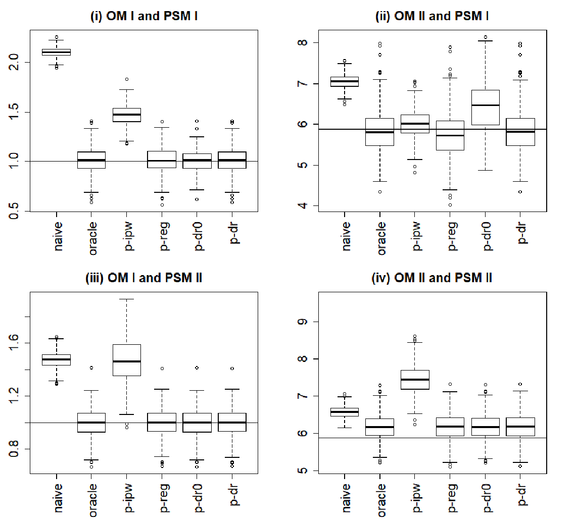
Figure 1 displays the estimation simulation results for the continuous outcome. The naive estimator shows large biases across scenarios. The oracle estimator is doubly robust, in the sense that if either the outcome or the sampling score is correctly specified, it is unbiased. The penalized inverse probability of sampling weighting estimator shows larges biases except for Scenario (ii). The weighted estimator is based on the blended sample combining Sample A and Sample B, where the units in Sample A are weighted by the known sampling weights and the units in Sample B are weighted by . This approach is justifiable only if the sampling rate of Sample B is relatively small compared the the population size. The penalized regression estimator is only singly robust. When the outcome model is misspecified as in Scenarios (ii) and (iv), it shows large biases. The proposed penalized double estimating equation estimator based on is doubly robust, and its performance is comparable to the oracle estimator that requires knowing the true important variables. Moreover, is slightly more efficient than . This efficiency gain is due to using the union of covariates selected for the sampling score model and the outcome model. This phenomenon is consistent with the findings in Brookhart et al. 2006 and Shortreed and Ertefaie 2017. The proposed penalized double estimating equation estimator based on is slightly more efficient than based on in Scenario (i) when both the outcome and sampling score models are correctly specified; however, has a large bias in Scenario (ii) when the outcome model is misspecified and therefore is not doubly robust anymore; see Remark 3.
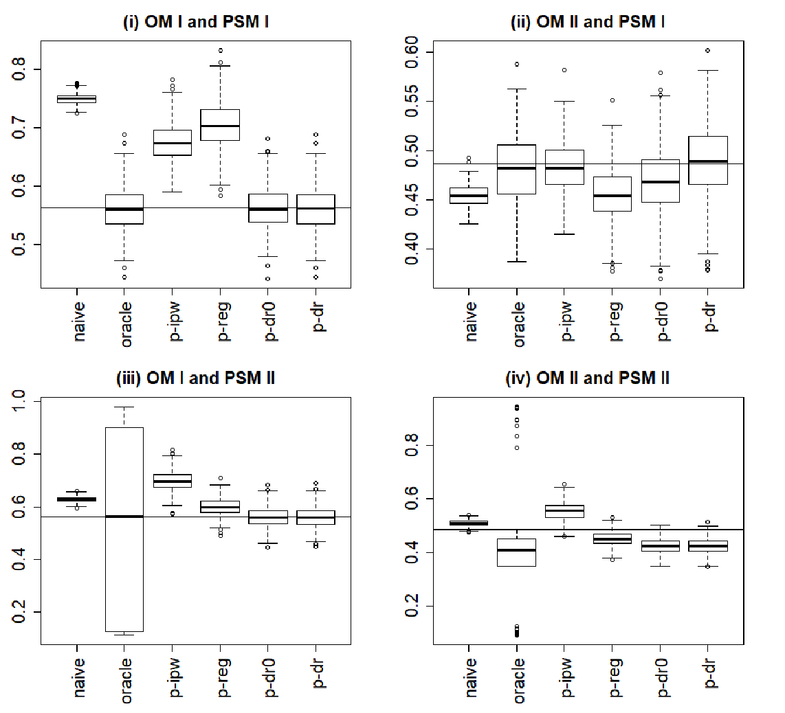
Figure 2 displays the estimation results for the binary outcome. The same discussion above applies here. Moreover, when the outcome model is incorrectly specified, the oracle estimator has a large variability. In this case, the proposed estimator outperforms the oracle estimator, because the variable selection step helps to stabilize the estimation performance.
Table 3 reports the simulation results for the coverage properties for the continuous outcome and binary outcome. Under the double robustness condition (i.e., if either the outcome model or the sampling score model is correctly specified), the coverage rates are close to the nominal coverage; while if both models are misspecified, the coverage rates are off the nominal coverage.
| Under | Over | FN | FP | Under | Over | FN | FP | ||
| Continuous outcome | |||||||||
| (i) OM I and PSM I | 0.0 | 31.8 | 0.0 | 1.4 | 0.0 | 0.0 | 0.0 | 0.0 | |
| (ii) OM II and PSM I | 70.6 | 15.0 | 0.9 | 0.2 | 0.0 | 0.0 | 0.0 | 0.0 | |
| (iii) OM I and PSM II | 0.0 | 32.8 | 0.0 | 1.4 | 100.0 | 100.0 | 4.0 | 1.0 | |
| (iv) OM II and PSM II | 0.0 | 0.4 | 0.0 | 0.4 | 100.0 | 100.0 | 3.5 | 4.3 | |
| Binary outcome | |||||||||
| (i) OM I and PSM I | 0.0 | 0.0 | 0.0 | 0.0 | 0.0 | 0.0 | 0.0 | 0.0 | |
| (ii) OM II and PSM I | 100.0 | 0.0 | 2.1 | 0.0 | 0.0 | 0.0 | 0.0 | 0.0 | |
| (iii) OM I and PSM II | 0.0 | 0.0 | 0.0 | 0.0 | 100.0 | 100.0 | 4.0 | 1.0 | |
| (iv) OM II and PSM II | 100.0 | 0.0 | 4.0 | 0.0 | 100.0 | 96.0 | 4.0 | 1.0 | |
| Continuous outcome | Binary outcome | ||||
|---|---|---|---|---|---|
| (i) OM I and PSM I | |||||
| (ii) OM II and PSM I | |||||
| (iii) OM I and PSM II | |||||
| (iv) OM II and PSM II | |||||
7 An Application

We analyze two datasets from the 2005 Pew Research Centre (PRC, http://www.pewresearch.org/) and the 2005 Behavioral Risk Factor Surveillance System (BRFSS). The goal of the PRC study was to evaluate the relationship between individuals and community (Chen, Li and Wu 2018, Kim et al. 2018). The 2005 PRC dataset is from a non-probability sample provided by eight different vendors, which consists of subjects. We focus on two study variables, a continuous (days had at least one drink last month) and a binary (an indicator of voted local elections). The 2005 BRFSS sample is a probability sample, which consists of subjects with survey weights. This dataset does not have measurements on the study variables of interest; however, it contains a rich set of common covariates with the PRC dataset listed in Figure 3. To illustrate the heterogeneity in the study populations, Figure 3 contrasts the covariate means from the PRC data and the design-weighted covariate means (i.e., the estimated population covariate means) from the BRFSS dataset. The covariate distributions from the PRC sample and the BRFSS sample are considerably different, e.g., age, education (high school or less), financial status (no money to see doctors, own house), retirement rate, and health (smoking). Therefore, the naive analyses of the study variables based on the PRC dataset are subject to selection biases.
We compute the naive and proposed estimators. To apply the proposed method, we assume the sampling score to be a logistic regression model, the continuous outcome to be a linear regression model, and the binary outcome model to be a logistic regression model adjusting for all available covariates. Using cross validation, the double selection procedure identifies 18 important covariates (all available covariates except for the northeast region) in the sampling score and the binary outcome model, and it identifies 15 important covariates (all available covariates except for black, indicator of smoking everyday, the northeast region and the south region).
Table 4 presents the point estimate and the standard error. For estimating the standard error, because the second-order inclusion probabilities are unknown, following the survey literature, we approximate the variance estimator in (32) by assuming the survey design is single-stage Poisson sampling. We find significant differences in the results between our proposed estimator and the corresponding naive estimator. As demonstrated by the simulation in Section 6, the naive estimator may be biased due to selection biases, and the proposed estimator utilizes a probability sample to correct for such biases. From the results, on average, the target population had at least one drink for days over the last month, and of the target population voted in local elections.
| (days had at least one drink last month) | (whether voted local elections) | ||||||
| Est | SE | CI | Est | SE | CI | ||
| Naive | 5.36 | 0.90 | (5.17,5.54) | 75.3 | 0.5 | (74.4,76.3) | |
| Proposed method | 4.84 | 0.15 | (4.81,4.87) | 71.8 | 0.2 | (71.3,72.2) | |
Acknowledgment
Dr. Yang is partially supported by the National Science Foundation grant DMS 1811245, National Cancer Institute grant P01 CA142538, and Oak Ridge Associated Universities. Dr. Kim is partially supported by the National Science Foundation MMS-1733572. An R package ”IntegrativeFPM” that implements the proposed method is available at https://github.com/shuyang1987/IntegrativeFPM.
SUPPLEMENTARY MATERIAL
Supplementary material provides technical details and proofs.
References
- (1)
- Bang and Robins (2005) Bang, H. and Robins, J. M. (2005). Doubly robust estimation in missing data and causal inference models, Biometrics 61: 962–973.
- Bethlehem (2016) Bethlehem, J. (2016). Solving the nonresponse problem with sample matching?, Social Science Computer Review 34: 59–77.
- Breidt et al. (1996) Breidt, F. J., McVey, A. and Fuller, W. A. (1996). Two-phase estimation by imputation, J. Indian Soc. Agri. Statist. 49: 79–90.
- Brookhart et al. (2006) Brookhart, M. A., Schneeweiss, S., Rothman, K. J., Glynn, R. J., Avorn, J. and Stürmer, T. (2006). Variable selection for propensity score models, Am. J. Epidemiol. 163: 1149–1156.
- Buchanan et al. (2018) Buchanan, A. L., Hudgens, M. G., Cole, S. R., Mollan, K. R., Sax, P. E., Daar, E. S., Adimora, A. A., Eron, J. J. and Mugavero, M. J. (2018). Generalizing evidence from randomized trials using inverse probability of sampling weights, J. R. Statist. Soc. A p. doi: 10.1111/rssa.12357.
- Cao et al. (2009) Cao, W., Tsiatis, A. A. and Davidian, M. (2009). Improving efficiency and robustness of the doubly robust estimator for a population mean with incomplete data, Biometrika 96: 723–734.
- Chen, Valliant and Elliott (2018) Chen, J. K. T., Valliant, R. and Elliott, M. R. (2018). Model-assisted calibration of non-probability sample survey data using adaptive LASSO, Survey Methodology 44: 117–144.
- Chen et al. (2019) Chen, J. K. T., Valliant, R. L. and Elliott, M. R. (2019). Calibrating non-probability surveys to estimated control totals using LASSO, with an application to political polling, Journal of the Royal Statistical Society: Series C (Applied Statistics) 68: 657–681.
- Chen, Li and Wu (2018) Chen, Y., Li, P. and Wu, C. (2018). Doubly robust inference with non-probability survey samples, arXiv preprint arXiv:1805.06432 .
- Chernozhukov et al. (2018) Chernozhukov, V., Chetverikov, D., Demirer, M., Duflo, E., Hansen, C., Newey, W. and Robins, J. (2018). Double/debiased machine learning for treatment and structural parameters, The Econometrics Journal 21: C1–C68.
- Chipperfield et al. (2012) Chipperfield, J., Chessman, J. and Lim, R. (2012). Combining household surveys using mass imputation to estimate population totals, Aust. New Zeal. J. Statist. 54: 223–238.
- De Luna et al. (2011) De Luna, X., Waernbaum, I. and Richardson, T. S. (2011). Covariate selection for the nonparametric estimation of an average treatment effect, Biometrika 98: 861–875.
- Deville and Särndal (1992) Deville, J.-C. and Särndal, C.-E. (1992). Calibration estimators in survey sampling, J. Am. Stat. Assoc. 87: 376–382.
- DiSogra et al. (2011) DiSogra, C., Cobb, C., Chan, E. and Dennis, J. M. (2011). Calibrating non-probability internet samples with probability samples using early adopter characteristics, Joint Statistical Meetings (JSM), Survey Research Methods, pp. 4501–4515.
- Elliott and Valliant (2017) Elliott, M. R. and Valliant, R. (2017). Inference for nonprobability samples, Statist. Sci. 32: 249–264.
- Fan and Li (2001) Fan, J. and Li, R. (2001). Variable selection via nonconcave penalized likelihood and its oracle properties, J. Am. Stat. Assoc. 96: 1348–1360.
- Fan and Lv (2011) Fan, J. and Lv, J. (2011). Nonconcave penalized likelihood with np-dimensionality, IEEE Trans. Inf. Theory 57: 5467–5484.
- Farrell (2015) Farrell, M. H. (2015). Robust inference on average treatment effects with possibly more covariates than observations, Journal of Econometrics 189: 1–23.
- Friedman et al. (2007) Friedman, J., Hastie, T., Höfling, H., Tibshirani, R. et al. (2007). Pathwise coordinate optimization, Ann. Appl. Statist. 1: 302–332.
- Fuller (2009) Fuller, W. A. (2009). Sampling Statistics, Wiley, Hoboken, NJ.
- Gao and Carroll (2017) Gao, X. and Carroll, R. J. (2017). Data integration with high dimensionality, Biometrika 104: 251–272.
- Han and Wang (2013) Han, P. and Wang, L. (2013). Estimation with missing data: beyond double robustness, Biometrika 100: 417–430.
- Hunter and Li (2005) Hunter, D. R. and Li, R. (2005). Variable selection using MM algorithms, Annals of Statistics 33: 1617–1642.
- Johnson et al. (2008) Johnson, B. A., Lin, D. and Zeng, D. (2008). Penalized estimating functions and variable selection in semiparametric regression models, J. Am. Stat. Assoc. 103: 672–680.
- Kang and Schafer (2007) Kang, J. D. and Schafer, J. L. (2007). Demystifying double robustness: A comparison of alternative strategies for estimating a population mean from incomplete data, Statist. Sci. 22: 523–539.
- Keiding and Louis (2016) Keiding, N. and Louis, T. A. (2016). Perils and potentials of self-selected entry to epidemiological studies and surveys, J. R. Statist. Soc. A 179: 319–376.
- Kim and Haziza (2014) Kim, J. K. and Haziza, D. (2014). Doubly robust inference with missing data in survey sampling, Statistica Sinica 24: 375–394.
- Kim et al. (2018) Kim, J. K., Park, S., Chen, Y. and Wu, C. (2018). Combining non-probability and probability survey samples through mass imputation, arxiv.org/abs/1812.10694 .
- Kim and Rao (2012) Kim, J. K. and Rao, J. N. K. (2012). Combining data from two independent surveys: a model-assisted approach, Biometrika 99: 85–100.
- Kott (2019) Kott, P. (2019). A partially successful attempt to integrate a web-recruited cohort into an address-based sample, Survey Research Methods pp. 95–101.
- Kott (2006) Kott, P. S. (2006). Using calibration weighting to adjust for nonresponse and coverage errors, Survey Methodology 32: 133–142.
- Lee and Valliant (2009) Lee, S. and Valliant, R. (2009). Estimation for volunteer panel web surveys using propensity score adjustment and calibration adjustment, Sociological Methods & Research 37: 319–343.
- McConville et al. (2017) McConville, K. S., Breidt, F. J., Lee, T. C. and Moisen, G. G. (2017). Model-assisted survey regression estimation with the LASSO, Journal of Survey Statistics and Methodology 5: 131–158.
- Meng (2018) Meng, X.-L. (2018). Statistical paradises and paradoxes in big data (I): Law of large populations, big data paradox, and the 2016 US presidential election, Ann. Appl. Statist. 12: 685–726.
- O’Muircheartaigh and Hedges (2014) O’Muircheartaigh, C. and Hedges, L. V. (2014). Generalizing from unrepresentative experiments: a stratified propensity score approach, J. R. Statist. Soc. C 63: 195–210.
- Patrick et al. (2011) Patrick, A. R., Schneeweiss, S., Brookhart, M. A., Glynn, R. J., Rothman, K. J., Avorn, J. and Stürmer, T. (2011). The implications of propensity score variable selection strategies in pharmacoepidemiology: an empirical illustration, Pharmacoepidemiology and Drug Safety 20: 551–559.
- Rivers (2007) Rivers, D. (2007). Sampling for web surveys, Proc. Survey Res. Meth. Sect., American Statistical Association.
- Rosenbaum and Rubin (1983) Rosenbaum, P. R. and Rubin, D. B. (1983). The central role of the propensity score in observational studies for causal effects, Biometrika 70: 41–55.
- Shao and Steel (1999) Shao, J. and Steel, P. (1999). Variance estimation for survey data with composite imputation and nonnegligible sampling fractions, J. Am. Stat. Assoc. 94: 254–265.
- Shortreed and Ertefaie (2017) Shortreed, S. M. and Ertefaie, A. (2017). Outcome-adaptive lasso: Variable selection for causal inference, Biometrics 73: 1111–1122.
- Stuart et al. (2015) Stuart, E. A., Bradshaw, C. P. and Leaf, P. J. (2015). Assessing the generalizability of randomized trial results to target populations, Prev. Sci. 16: 475–485.
- Stuart et al. (2011) Stuart, E. A., Cole, S. R., Bradshaw, C. P. and Leaf, P. J. (2011). The use of propensity scores to assess the generalizability of results from randomized trials, J. R. Statist. Soc. A 174: 369–386.
- Tsiatis (2006) Tsiatis, A. (2006). Semiparametric Theory and Missing Data, Springer, New York.
- Valliant and Dever (2011) Valliant, R. and Dever, J. A. (2011). Estimating propensity adjustments for volunteer web surveys, Sociological Methods & Research 40: 105–137.
- Yang and Kim (2018) Yang, S. and Kim, J. K. (2018). Integration of survey data and big observational data for finite population inference using mass imputation, arXiv preprint arXiv:1807.02817 .