Ribosome flow model with different site sizes

Eyal Bar-Shalom Alexander Ovseevich Michael Margaliot Thanks: E. Bar-Shalom is with the School of Electrical Engineering, Tel-Aviv University, Tel-Aviv 69978, Israel. E-mail: eyalbarshalom500@gmail.com A. Ovseevich is with the Ishlinsky Institute for Problems in Mechanics, Russian Academy of Sciences and the Russian Quantum Center, Moscow, Russia. E-mail: ovseev@ipmnet.ru M. Margaliot (corresponding author) is with the School of Electrical Engineering and the Sagol School of Neuroscience, Tel-Aviv University, Tel-Aviv 69978, Israel. E-mail: michaelm@eng.tau.ac.il

Abstract

We introduce and analyze two general dynamical models for unidirectional movement of particles along a circular chain and an open chain of sites. The models include a soft version of the simple exclusion principle, that is, as the density in a site increases the effective entry rate into this site decreases. This allows to model and study the evolution of “traffic jams” of particles along the chain. A unique feature of these two new models is that each site along the chain can have a different size.

Although the models are nonlinear, they are amenable to rigorous asymptotic analysis. In particular, we show that the dynamics always converges to a steady-state, and that the steady-state densities along the chain and the steady-state output flow rate from the chain can be derived from the spectral properties of a suitable matrix, thus eliminating the need to numerically simulate the dynamics until convergence. This spectral representation also allows for powerful sensitivity analysis, i.e. understanding how a change in one of the parameters in the models affects the steady-state.

We show that the site sizes and the transition rates from site to site play different roles in the dynamics, and that for the purpose of maximizing the steady-state output (or production) rate the site sizes are more important than the transition rates. We also show that the problem of finding parameter values that maximize the production rate is tractable.

We believe that the models introduced here can be applied to study various natural and artificial processes including ribosome flow during mRNA translation, the movement of molecular motors along filaments of the cytoskeleton, pedestrian and vehicular traffic, evacuation dynamics, and more.

I Introduction

Understanding various transport phenomena in the cell is of considerable interest. Fundamental cellular processes like transcription, translation, and the movement of molecular motors can be studied using a general model for the flow of “particles” along a cellular “track”. The particles may be ribosomes moving along the mRNA strand or molecular motors moving along actin filaments. To increase the flow, often several particles traverse the same track simultaneously. For example, during mRNA translation several ribosomes may “read” the same mRNA strand simultaneously (thus forming a polysome). It is important to note that new experimental methods are providing unprecedented data on the dynamics of this fundamental biological process [1], thus increasing the interest in computational models that can integrate and explain this data.

A simple physical concept underlying such motion is the simple exclusion principle: two particles cannot be in the same site along the track at the same time. This implies that a “traffic jam” of particles may evolve behind a particle that remains in the same site for a long time. The evolution and implications of such traffic jams in various biological processes are attracting considerable interest (see, e.g. [24, 2, 27]).

To study the transport phenomena in the cell in a qualitative and quantitative manner, scientists build computational models, identify useful control parameters, and determine the functional dependence of the transport properties on these parameters. Such models are particularly important in the context of synthetic biology and biomimetic systems where biological modules are modified or redesigned [29]. An important goal in such studies is to determine how the density of particles along the chain depends on the structure and parameters of the system, and to find parameter values that lead to an optimal production rate [33, 6, 7, 32].

A fundamental model from statistical physics is the totally asymmetric simple exclusion process (TASEP) [25, 36, 10]. This is a stochastic model for unidirectional movement that takes place on some kind of tracks or trails. The tracks are modeled by an ordered lattice of sites, and the moving objects are modeled as particles that can hop, with some probability, from one site to the consecutive site. The motion is assumed to be asymmetric in the sense that there is some preferred direction of motion. The term totally asymmetric refers to the case where motion is unidirectional. The term simple exclusion refers to the fact that hops to a target site may take place only if it is not already occupied by another particle. Note that every site may either by empty or contain a single particle, so in particular all the sites have the same size.

TASEP has two basic configurations, open boundary conditions and periodic boundary conditions. In the first configuration, the lattice boundaries are open and the first and last sites are connected to external particle reservoirs. In TASEP with periodic boundary conditions, the lattice is closed, so that a particle that hops from the last site returns back to the first one. Thus, the particles hop around a circular chain, and the total number of particles along the lattice is conserved.

In this paper, we introduce and rigorously analyze two nonlinear continuous-time dynamical models describing the unidirectional movement of “particles” along a circular and an open chain of $n$ sites. For every index $i\in\{1,\dots,n\}$ site $i$ has a size site (i.e. maximal possible capacity) $q_{i}$ , and the transition to site $i+1$ is controlled by a parameter $\lambda_{i}$ . The state-variable $x_{i}(t)$ , that takes values in $[0,q_{i}]$ , describes the density of particles at site $i$ at time $t$ . The models include a soft version of the simple exclusion principle. This allows to study the evolution of “traffic jams” along the chain and, in particular, the effect of a small transition rate $\lambda_{i}$ or a small site size $q_{i}$ . A unique feature of these models is that each site along the chain can have a different size. Indeed, there is no a priori reason to expect that the capacity in two different sites is equal. For example, if we consider the flow of vehicular traffic along a road then the capacity changes when the number of parallel lanes along the road increases or decreases.

Although nonlinear, the new models are amenable to rigorous analysis. Our results show that the dynamics always converges to a steady-state. In other words, as time goes to infinity, the density $x_{i}(t)$ at every site $i\in\{1,\dots,n\}$ converges to a steady-state value $e_{i}$ , with $e_{i}\in[0,q_{i}]$ . This means that as time goes to infinity, the effective entry rate into site $i$ and the effective exit rate from site $i$ become equal, yielding a constant density $e_{i}$ at site $i$ . In the open chain, these steady-state densities depend on all the parameters $q_{i},\lambda_{i}$ , but not on the initial density $x_{j}(0)$ , $j=1,\dots,n$ , at each site. In the circular model, the steady-state densities depend on all the parameters $q_{i},\lambda_{i}$ , and also on the initial total density, i.e. $x_{1}(0)+\dots+x_{n}(0)$ along the chain.

Surprisingly, we show that in both models the steady-state densities and flow rate can be derived from the spectral properties of a suitable matrix, thus eliminating the need to numerically simulate the dynamics until convergence. This spectral representation also allows a powerful sensitivity analysis, i.e. understanding how a change in one of the parameters in the models affects the steady-state. Furthermore, we apply the spectral representation to show that the mapping from the model parameters to the steady-state flow rate is quasi-concave implying that the problem of maximizing the flow rate is numerically tractable even for very long chains.

The remainder of this paper is organized as follows. The next section reviews several related models and in particular emphasizes the unique features of the new models introduced here. Section III describes the two new models for movement along a circular and an open chain. The main analysis results are described in Sections IV and V. We first analyze the circular model and then show that the steady-state behavior in the open model can be derived by taking one of the transition rates $\lambda_{i}$ in the $n$ -dimensional circular model to infinity. This effectively “opens the loop” in the circular model yielding an open model with dimension $n-2$ . The final section concludes and describes several directions for further research.

II Preliminaries

The ribosome flow model (RFM) [23] is a dynamic mean-field approximation of TASEP with open boundary conditions. The RFM has been extensively used to model and analyze ribosome flow along an mRNA molecule [11, 12, 13, 14, 19, 30, 31, 33]. The molecule is coarse-grained into $n$ codons (or groups of codons). Ribosomes reach the first site with initiation rate $\lambda_{0}>0$ , but the effective entry rate decreases as the density in the first site increases. A ribosome that occupies site $i$ moves, with transition rate $\lambda_{i}>0$ , to the consecutive site but again the effective rate decreases as the consecutive site becomes more occupied.

The ribosome flow model on a ring (RFMR) [21, 35] is the dynamic mean-field of TASEP with periodic boundary conditions. Here the particles exiting the last site enter the first site. The RFMR dynamics admits a first integral as the total density along the chain is preserved. The RFMR has been used as a model for mRNA translation with ribosome recycling. Note that a recent study [17] concluded that polysomes are globular in shape rather than elongated, based on the observation that the distance between protein- and mRNA-labeling fluorophores was largely unaffected by the length of the coding sequence.

In both the RFM and RFMR all the sites along the chain are assumed to have the same size, and this is normalized to one. Here, we introduce and analyze generalizations of these models, called the RFM with different site sizes and RFMR with different site sizes, respectively, that allow for different site sizes.

III New Models

We begin with the open model, i.e. the RFM with different site sizes (RFMD) depicted in Fig. 1. This is described by $n$ first-order differential equations:

$\displaystyle\dot{x}_{1}$	$\displaystyle=\lambda_{0}(q_{1}-x_{1})-\lambda_{1}x_{1}(q_{2}-x_{2}),$
$\displaystyle\dot{x}_{2}$	$\displaystyle=\lambda_{1}x_{1}(q_{2}-x_{2})-\lambda_{2}x_{2}(q_{3}-x_{3}),$

$\displaystyle\dot{x}_{n}$	$\displaystyle=\lambda_{n-1}x_{n-1}(q_{n}-x_{n})-\lambda_{n}x_{n},$	(1)

with $\lambda_{i}>0$ and $0<q_{i}\leq 1$ for all $i$ . The state variable $x_{i}(t):\mathbb{R}_{+}\rightarrow[0,q_{i}]$ , $i=1,...,n$ , describes the normalized occupancy level at site $i$ at time $t$ , where $x_{i}(t)=q_{i}$ $[x_{i}(t)=0]$ indicates that site $i$ is completely full [empty] at time $t$ .

The model includes $2n+1$ positive parameters. The parameters $\lambda_{0},\dots,\lambda_{n}$ describe the maximal possible transition rate between the sites: the initiation rate $\lambda_{0}$ into the chain, the elongation (or transition) rate $\lambda_{i}$ from site $i$ to site $i+1$ , $i=1,...,n-1$ , and the exit rate $\lambda_{n}$ . The parameters $q_{1},\dots,q_{n}\in(0,1]$ describe the maximal capacity at each site. The use of different values $q_{i}$ allows to model flow through a chain of sites with different sizes. In the special case where $q_{i}=1$ for all $i=1,\dots,n$ we retrieve the RFM that has been extensively used to model and analyze the flow of ribosomes along the mRNA molecule during translation (see, e.g. [23, 34, 22, 32]).

Refer to caption — Fig. 1: The RFM with different site sizes models unidirectional flow along a chain of $n$ sites. The state variable $x_{i}(t)\in[0,q_{i}]$ represents the density at site $i$ at time $t$ . The maximal possible density at site $i$ is $q_{i}$ . The parameter $\lambda_{i}>0$ controls the transition rate from site $i$ to site $i+1$ , with $\lambda_{0}>0$ [ $\lambda_{n}>0$ ] controlling the initiation [exit] rate. The output rate at time $t$ is $R(t):=\lambda_{n}x_{n}(t)$ .

It is important to note that the RFMD cannot be derived by simply scaling the state-variables in the RFM. The next example demonstrates this.

Example 1

Consider an RFM with $n=2$ , i.e.

	$\displaystyle\dot{x}_{1}$	$\displaystyle=\lambda_{0}(1-x_{1})-\lambda_{1}x_{1}(1-x_{2}),$
	$\displaystyle\dot{x}_{2}$	$\displaystyle=\lambda_{1}x_{1}(1-x_{2})-\lambda_{2}x_{2}.$

Define new state-variables $z_{i}(t):=s_{i}x_{i}(t)$ , with $s_{i}>0$ . Then the equations in the new state-variables are:

	$\displaystyle\dot{z}_{1}$	$\displaystyle=\lambda_{0}(s_{1}-z_{1})-\frac{\lambda_{1}}{s_{2}}z_{1}(s_{2}-z_{2}),$
	$\displaystyle\dot{z}_{2}$	$\displaystyle=\frac{\lambda_{1}}{s_{1}}z_{1}(s_{2}-z_{2})-\lambda_{2}z_{2}.$		(2)

If $s_{1}\not=s_{2}$ then (1) is not an RFMD, as the flow out of site $1$ is $\frac{\lambda_{1}}{s_{2}}z_{1}(s_{2}-z_{2})$ whereas the flow into site $2$ is $\frac{\lambda_{1}}{s_{1}}z_{1}(s_{2}-z_{2})$ , and these are not equal. If $s_{1}=s_{2}$ then (1) is also not a general RFMD, as both sites have the same size, namely, $s_{1}=s_{2}$ .

The different site sizes in the RFMD add important dynamical features that do not exist in the RFM nor other equal-site models like TASEP. The next example demonstrates this.

Example 2

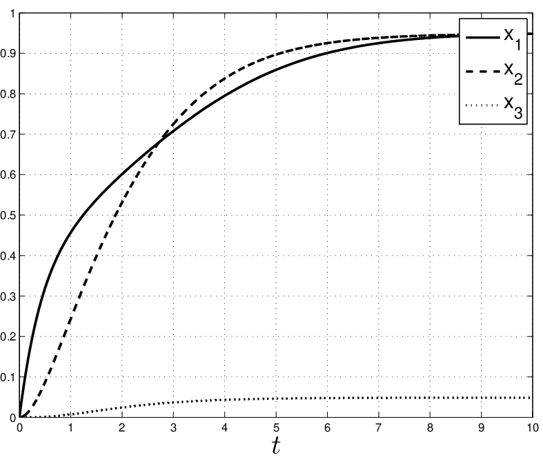
Fig. 2 depicts the state-variables $x_{i}(t)$ , $i=1,2,3$ , in an RFMD with $n=3$ and compares them to the state-variables in an RFM with $n=3$ . In both models all the $\lambda_{i}$ ’s are set to one. In the RFMD the site sizes are $q_{1}=q_{2}=1$ , and $q_{3}=0.1$ . Thus, the last site has a much smaller size than the first two.

It may be seen that in both models the state-variables converge to a steady-state. However, the steady-state behavior in the two models is quite different. The small size of site $3$ in the RFMD makes it fill up quickly. Consequently, site $2$ fills up and then also site $1$ . This generates a “traffic jam” in the RFMD. Thus, in the RFMD there can be two different “bottlenecks” that generate traffic jams: a small transition rate or a small site size.

We now turn to describe the RFMRD. This is similar to the RFMD, but under the additional assumption that all the particles leaving site $n$ circulate back to site $1$ . The equations are thus:

$\displaystyle\dot{x}_{1}$	$\displaystyle=\lambda_{n}x_{n}(q_{1}-x_{1})-\lambda_{1}x_{1}(q_{2}-x_{2}),$
$\displaystyle\dot{x}_{2}$	$\displaystyle=\lambda_{1}x_{1}(q_{2}-x_{2})-\lambda_{2}x_{2}(q_{3}-x_{3}),$

$\displaystyle\dot{x}_{n}$	$\displaystyle=\lambda_{n-1}x_{n-1}(q_{n}-x_{n})-\lambda_{n}x_{n}(q_{1}-x_{1}).$	(3)

Note that here the entry rate into site $1$ is equal to the exit rate from site $n$ . This models a flow of particles along a circular chain, rather than an open chain. When considering the RFMRD we always interpret the indexes modulo $n$ . For example, $\lambda_{n+1}=\lambda_{1}$ and $q_{0}=q_{n}$ .

In the special case where $q_{i}=1$ for all $i$ the RFMRD in (III) becomes the ribosome flow model on a ring (RFMR) that has been used to study ribosome flow with circularization [21, 35, 33].

The next two sections describe the mathematical properties of the new models. We begin by analyzing the RFMRD, as we will later show that the theoretical results for the RFMD follow by taking $\lambda_{n}\to\infty$ in an RFMRD with a specific total density. To increase readability, all the proofs are placed in the Appendix.

IV Analysis of the RFMRD

The state space of (III) is the set $C:=[0,q_{1}]\times\dots\times[0,q_{n}]$ . For any initial condition $a\in C$ , let $x(t,a)$ denote the solution at time $t$ of (III) with $x(0)=a$ . Define the function $H:\mathbb{R}^{n}_{+}\to\mathbb{R}_{+}$ by $H(y):=y_{1}+\dots+y_{n}.$ An important property of (III) is that $\sum_{i=1}^{n}\dot{x}_{i}(t)\equiv 0$ . This means that along any solution of (III) we have

H(x(t,a))\equiv H(a).

In other words, the total density along the circular chain is conserved. For $s\in[0,q_{1}+\dots+q_{n}]$ , let

L_{s}:=\{y\in C:\sum_{i=1}^{n}y_{i}=s\}

denote the $s$ level-set of $H$ , i.e. the set of all points $y\in C$ such that $H(y)=s$ . For example, for $n=2$ and $s=3$ the set $L_{3}$ includes the points $\begin{bmatrix}0&3\end{bmatrix}^{T}$ , $\begin{bmatrix}0.5&2.5\end{bmatrix}^{T}$ , and so on.

IV-A Invariance and asymptotic stability

The next result shows that for any $a\in C$ the solution $x(t,a)$ of the RFMRD remains in $C$ for all $t\geq 0$ . In other words, for any $i$ , the density $x_{i}(t)\in[0,q_{i}]$ for any time $t\geq 0$ . This means that the density remains well-defined for all $t\geq 0$ . Furthermore, $x(t,a)$ converges to a steady-state that depends on the RFMRD parameters and on the initial total density $x_{1}(0)+\dots+x_{n}(0)$ . Recall that all the proofs are placed in the Appendix.

Proposition 1

The set $C$ is an invariant set of (III). For any $s\in[0,q_{1}+\dots+q_{n}]$ the set $L_{s}$ includes a unique steady-state $e^{s}$ and any solution $x(t,a)$ of (III) with $\sum_{i=1}^{n}a_{i}(0)=s$ satisfies

\lim_{t\to\infty}x(t,a)=e^{s}.

Example 3

Consider the RFMRD with $n=3$ , $\lambda_{1}=\lambda_{2}=\lambda_{3}=1$ , $q_{1}=1$ , $q_{2}=1/2$ , and $q_{3}=1$ . Fig. 4 depicts the trajectories emanating from three different initial conditions in the level set $L_{1}$ : $\begin{bmatrix}1/3&1/3&1/3\end{bmatrix}^{T}$ , $\begin{bmatrix}2/5&1/5&2/5\end{bmatrix}^{T}$ , and $\begin{bmatrix}1/3&1/2&1/6\end{bmatrix}^{T}$ . It may be observed that all three trajectories converge to the same equilibrium point $e^{1}=\begin{bmatrix}0.5&0.207&0.293\end{bmatrix}^{T}$ (all numerical values in this paper are to four-digit accuracy).

It is clear that $e^{s}$ satisfies $\sum_{i=1}^{n}e_{i}^{s}=s$ , and also

$\displaystyle\lambda_{n}e_{n}^{s}(q_{1}-e_{1}^{s})$	$\displaystyle=\lambda_{1}e_{1}^{s}(q_{2}-e_{2}^{s})$	(4)
	$\displaystyle=\lambda_{2}e_{2}^{s}(q_{3}-e_{3}^{s})$

	$\displaystyle=\lambda_{n-1}e_{n-1}^{s}(q_{n}-e_{n}^{s}).$

In other words, at the steady-state the flow into and out of each site is equal. Let

\displaystyle R^{s}:=\lambda_{n-1}e_{n-1}^{s}(q_{n}-e_{n}^{s})

denote this steady-state flow rate for any initial condition in $L_{s}$ .

Note that $L_{0}$ includes only the origin and for this initial condition $x(t)\equiv 0$ , so $e^{0}=0$ , and $R^{0}=0$ . Let $p:=q_{1}+\dots+q_{n}$ . Then $L_{p}$ includes only the point $q:=\begin{bmatrix}q_{1}&\dots&q_{n}\end{bmatrix}^{\prime}$ and for this initial condition $e^{p}=q$ , and $R^{p}=0$ . Thus, the steady-state flow is zero in both these extreme cases.

IV-B Optimal steady-state flow

A natural question is how does $R^{s}$ depends on $s$ ? When $s$ is very small we expect a small $R^{s}$ because there are few particles along the circular chain. When $s$ is very large we again expect a small $R^{s}$ because there are too many particles along the circular chain and this yields “traffic jams”. The next result shows that there exists a unique total density $s^{*}$ that maximizes the steady-state flow rate. We refer to this as the optimal density.

Proposition 2

Consider an RFMRD with rates $\lambda_{i}$ and site sizes $q_{i}$ . There exists a unique value $s^{*}=s^{*}(\lambda_{1},\dots,\lambda_{n},q_{1},\dots,q_{n})\in[0,q_{1}+\dots+q_{n}]$ such that $R^{*}:=R^{s^{*}}>R^{s}$ for any $s\not=s^{*}$ . Furthermore, $R^{s}$ is increasing in $s$ for all $s<s^{*}$ and decreasing in $s$ for all $s>s^{*}$ . Let $e^{*}$ denote the steady-state corresponding to the density $s^{*}$ . Then

e_{1}^{*}e_{2}^{*}\dots e_{n}^{*}=(q_{1}-e_{1}^{*})(q_{2}-e_{2}^{*})\dots(q_{n}-e_{n}^{*}).

(5)

Eq. (5) can be explained as follows. If $s$ is very small, then every $e_{i}^{s}$ is small (as $\sum_{i=1}^{n}e_{i}^{s}=s$ ) and the left-hand side of (5) is smaller than the right-hand side. If $s$ is very large, then the opposite case occurs. The optimal $s^{*}$ is the value that yields an equality in (5).

Example 4

Fig. 5 depicts the steady-state flow rate $R^{s}$ as a function of $s$ for an RFMRD with $n=3$ , $\lambda_{1}=\lambda_{2}=\lambda_{3}=1$ , $q_{1}=1$ , $q_{2}=1/2$ , and $q_{3}=1$ . This was generated by simulating the dynamics until convergence for various values of $s$ with an initial condition $x(0)$ satisfying $x_{i}(0)\in[0,q_{i}]$ and $\sum_{i=1}^{3}x_{i}(0)=s$ . The value that maximizes $R^{s}$ is $s^{*}=1.25$ (i.e. one half of the maximal possible total density which is $q_{1}+q_{2}+q_{3}=2.5$ ), and the corresponding steady-state is

e_{1}^{*}=0.6096,\;e_{2}^{*}=0.2500,\;e_{3}^{*}=0.3904.

(6)

A calculation shows that these values satisfy (5). Note that here site $2$ is the “bottleneck site” in the sense that its size is smaller than that of the other two sites, and that $e^{*}_{2}=q_{2}/2$ , i.e. the optimal density at site $2$ is exactly one half of its capacity.

Example 5

Consider an RFMRD of order $n=2$ ,

	$\displaystyle\dot{x}_{1}$	$\displaystyle=\lambda_{2}x_{2}(q_{1}-x_{1})-\lambda_{1}x_{1}(q_{2}-x_{2}),$
	$\displaystyle\dot{x}_{2}$	$\displaystyle=\lambda_{1}x_{1}(q_{2}-x_{2})-\lambda_{2}x_{2}(q_{1}-x_{1}).$

The steady-state satisfies $\lambda_{2}e_{2}(q_{1}-e_{1})=\lambda_{1}e_{1}(q_{2}-e_{2}),$ and this yields

e_{2}=\frac{\lambda_{1}e_{1}q_{2}}{(\lambda_{1}-\lambda_{2})e_{1}+\lambda_{2}q_{1}}.

(7)

The steady-state flow rate is thus

	$\displaystyle R$	$\displaystyle=\lambda_{2}e_{2}(q_{1}-e_{1})$
		$\displaystyle=\frac{\lambda_{1}\lambda_{2}e_{1}q_{2}(q_{1}-e_{1})}{(\lambda_{1}-\lambda_{2})e_{1}+\lambda_{2}q_{1}}.$

Differentiating this expression with respect to $e_{1}$ and setting the result to zero yields two solutions for $e_{1}$ . The feasible one (i.e. the one in $[0,q_{1}]$ ) is

e_{1}^{*}=\frac{q_{1}}{1+\sqrt{\frac{\lambda_{1}}{\lambda_{2}}}}.

It is straightforward to verify that this corresponds to a maximum of $R$ . Now (7) yields

\displaystyle e_{2}^{*}=\frac{q_{2}}{1+\sqrt{\frac{\lambda_{2}}{\lambda_{1}}}},

and it is straightforward to verify that indeed

e_{1}^{*}e_{2}^{*}=(q_{1}-e_{1}^{*})(q_{2}-e_{2}^{*}).

Note also that here $e_{i}^{*}=c_{i}(\lambda_{1},\lambda_{2})q_{i}$ , with $c_{i}\in(0,1)$ . This means that the optimal density at site $i$ increases with $q_{i}$ . Also, $e_{1}^{*}$ decreases and $e_{2}^{*}$ increases when the ratio $\lambda_{1}/\lambda_{2}$ increases. This makes sense, as $\lambda_{1}$ controls the exit rate from site $1$ and the input rate into site $2$ , whereas $\lambda_{2}$ controls the input rate into site $1$ and the exit rate from site $2$ .

So far we determined $e^{*}$ and $R^{*}$ by solving equations (4) and (5). These equations are nonlinear and furthermore they provide little insight on the properties of $e^{*},R^{*}$ . It turns out that there is a different and more useful representation of the optimal steady-state values. This representation depends on the Perron root and Perron vector of a specific componentwise nonnegative matrix.

Given the RFMRD (III), define a parameter-dependent matrix $A:\mathbb{R}_{+}\to\mathbb{R}^{n\times n}$ by

A(\kappa):=\kappa D(q)+B(\lambda),

(8)

where $D(q)$ is the diagonal matrix with entries $1-q_{1},1-q_{2},...,1-q_{n}$ on the diagonal, and

B(\lambda):=\left[\begin{smallmatrix}0&\lambda_{1}^{-1/2}&0&0&\dots&0&\lambda_{n}^{-1/2}\\ \lambda_{1}^{-1/2}&0&\lambda_{2}^{-1/2}&0&\dots&0&0\\ 0&\lambda_{2}^{-1/2}&0&\lambda_{3}^{-1/2}&\dots&0&0\\ &&&\vdots\\ 0&0&0&\dots&\lambda_{n-2}^{-1/2}&0&\lambda_{n-1}^{-1/2}\\ \lambda_{n}^{-1/2}&0&0&\dots&0&\lambda_{n-1}^{-1/2}&0\end{smallmatrix}\right].

(9)

Note that $B$ is componentwise nonnegative and irreducible. Matrices in the form (8) are sometimes called periodic Jacobi matrices (see, e.g. [3]). We emphasize that the parameters $q_{i}$ and $\lambda_{i}$ in $D(q)$ and $B(\lambda)$ are the site sizes and transition rates of (III).

The matrix $A(\kappa)$ is componentwise nonnegative and irreducible for all $\kappa\geq 0$ and the Perron-Frobenius theory [4] implies that it admits a simple eigenvalue $\sigma(\kappa):=\sigma(A(\kappa))$ that is positive and larger than the modulus of any other eigenvalue. Let $\zeta(\kappa)\in\mathbb{R}^{n}_{++}$ denote the corresponding Perron vector, that is, $A(\kappa)\zeta(\kappa)=\sigma(\kappa)\zeta(\kappa)$ .

Theorem 1

Consider the RFMRD with $n>2$ . There exists a unique value $\kappa^{*}\in[0,\infty)$ such that the matrix $A(\kappa)$ satisfies

\sigma(\kappa^{*})=\kappa^{*}.

(10)

The optimal steady-state densities $e^{*}$ and flow rate $R^{*}$ of (III) satisfy

R^{*}=(\sigma(\kappa^{*}))^{-2}=(\kappa^{*})^{-2},

(11)

and

e^{*}_{i}=\frac{\zeta_{i+1}(\kappa^{*})}{\lambda_{i}^{1/2}\sigma(\kappa^{*})\zeta_{i}(\kappa^{*})},\quad i=1,\dots,n,

(12)

(recall that all indexes are interpreted modulo $n$ , so in particular $\zeta_{n+1}(\kappa^{*})=\zeta_{1}(\kappa^{*})$ ).

This provides a spectral representation for $e^{*}$ and $R^{*}$ in RFMRD. The proof of Thm. 1 (see the Appendix) uses the function

f(\kappa):=\sigma(A(\kappa))-\kappa,

(13)

and shows that $f(0)>0$ , $\lim_{\kappa\to\infty}f(\kappa)=-\infty$ and $\frac{d}{d\kappa}f(\kappa)<0$ for all $\kappa\geq 0$ . This implies that there exists a unique value $\kappa^{*}$ as described above, and also that it is easy to numerically determine $\kappa^{*}$ using for example a simple bisection algorithm.

Let $\eta>0$ denote the Perron root of $B(\lambda)$ . If $q_{i}=1$ for all $i$ then (8) gives $\sigma(A(\kappa))=\eta$ for all $\kappa$ , so the solution of (10) is $\kappa^{*}=\eta$ and (11) becomes $R^{*}=\eta^{-2}$ . This recovers the spectral representation of the steady-state in the RFMR [35]. Note however that the spectral representation of the steady-state in the RFMRD is quite different than the one in the RFMR as it includes two steps: determining the value $\kappa^{*}$ and then using the Perron root and Perron vector of $A(\kappa^{*})$ .

The next two examples demonstrate Thm. 1.

Example 6

Consider an RFMRD with $n=3$ . Recall that the optimal steady-state solution satisfies:

	$\displaystyle\lambda_{3}e_{3}^{}(q_{1}-e^{}_{1})$	$\displaystyle=\lambda_{1}e^{}_{1}(q_{2}-e^{}_{2})=\lambda_{2}e^{}_{2}(q_{3}-e^{}_{3})$		(14)
	$\displaystyle e_{1}^{}e_{2}^{}e_{3}^{*}$	$\displaystyle=(q_{1}-e_{1}^{})(q_{2}-e_{2}^{})(q_{3}-e_{3}^{*}).$		(15)

For $\lambda_{1}=\lambda_{2}=\lambda_{3}=1$ , $q_{1}=q_{3}=1$ and $q_{2}=1/2$ the feasible solution of (14) (i.e. the solution satisfying $e^{*}_{i}\in[0,q_{i}]$ for all $i$ ) is

e_{1}^{*}=\frac{9-\sqrt{17}}{8}\approx 0.6096,\;e_{2}^{*}=\frac{1}{4},\;e_{3}^{*}=\frac{-1+\sqrt{17}}{8}\approx 0.3904.

(16)

The steady-state optimal flow rate is thus

\displaystyle R^{*}=\lambda_{2}e^{*}_{2}(q_{3}-e^{*}_{3})=\frac{1}{32}(9-\sqrt{17})\approx 0.1524.

(17)

On the other hand, for these parameter values the matrix in (8) is $A(\kappa)=\begin{bmatrix}0&1&1\\ 1&\kappa/2&1\\ 1&1&0\end{bmatrix}.$ The Perron root of $A(\kappa)$ is $(2+\kappa+\sqrt{36-4\kappa+\kappa^{2}})/4$ , so $\kappa^{*}\geq 0$ is the solution of

\kappa=(2+\kappa+\sqrt{36-4\kappa+\kappa^{2}})/4

yielding $\kappa^{*}=(1+\sqrt{17})/2$ . Thus, Thm. 1 implies that

R^{*}=(\sigma(\kappa^{*}))^{-2}=((1+\sqrt{17})/2)^{-2}\approx 0.1524,

and this agrees with (17). The Perron vector of $A(\kappa^{*})$ is $\zeta(\kappa^{*})=\begin{bmatrix}5+\sqrt{17}&2(3+\sqrt{17})&5+\sqrt{17}\end{bmatrix}^{T},$ so Thm. 1 yields

	$\displaystyle e_{1}^{*}$	$\displaystyle=\frac{4(3+\sqrt{17})}{(5+\sqrt{17})(1+\sqrt{17})}\approx 0.6096,$
	$\displaystyle e_{2}^{*}$	$\displaystyle=\frac{5+\sqrt{17}}{(3+\sqrt{17})(1+\sqrt{17})}=1/4,$
	$\displaystyle e_{3}^{*}$	$\displaystyle=\frac{2}{1+\sqrt{17}}\approx 0.3904,$

and this agrees with (16).

Example 7

Consider the special case of an RFMRD with all the $q_{i}$ ’s equal and denote their common value by $q$ . Then $A(\kappa)=(1-q)\kappa I+B(\lambda)$ . Let $\eta>0$ denote the Perron root of $B$ . Then the Perron root of $A(\kappa)$ is $\sigma(\kappa)=(1-q)\kappa+\eta$ , so the equation $\sigma(\kappa)=\kappa$ becomes $(1-q)\kappa+\eta=\kappa$ and this admits a unique solution

\kappa^{*}=\eta/q.

(18)

The Perron vector $\zeta^{*}:=\zeta(k^{*})$ of $A^{*}:=A(\kappa^{*})$ satisfies $A^{*}\zeta^{*}=\kappa^{*}\zeta^{*}$ and this gives $B\zeta^{*}=\eta\zeta^{*}$ . Thus, $\zeta^{*}$ is the Perron vector of $B$ . If, in addition, all the $\lambda_{i}$ ’s are equal, with $\lambda$ denoting their common value, then it is straightforward to verify that the Perron root and vector of $B$ are $\eta=2\lambda^{-1/2}$ and $\mu:=\begin{bmatrix}1&\dots&1\end{bmatrix}^{T}$ . We conclude that if $q_{1}=\dots=q_{n}=q$ and $\lambda_{1}=\dots=\lambda_{n}=\lambda$ then $\kappa^{*}=2\lambda^{-1/2}/q$ , and $\zeta^{*}=\begin{bmatrix}1&\dots&1\end{bmatrix}^{T}$ , so the spectral representation yields

e_{i}^{*}=q/2\text{ for all }i,\text{ and }R^{*}=q^{2}\lambda/4.

(19)

Note that in this case the optimal steady-state density and flow rate do not depend on $n$ (yet the optimal total density $s^{*}$ does depend on $n$ , as $s^{*}=\sum_{i=1}^{n}q/2=qn/2$ ). It is important to note that (19) shows that $\lambda$ and $q$ play a very different role in determining $R^{*}$ . In particular, a small value of $q\in(0,1]$ will decrease $R^{*}$ more than a small value of $\lambda$ .

It is intuitively clear that even if one of the rates in the RFMRD goes to infinity the densities and production rate remain bounded, as the other rates constrain the dynamics. The next result states this formally for the optimal density case. As we will see below this will prove useful in analyzing the RFMD.

Corollary 1

The optimal-density production rate and densities in the RFMRD remain bounded if $\lambda_{i}\to\infty$ for some $i$ .

The spectral representation of the optimal steady-state in the RFMRD has important theoretical and practical implications. Two of these are discussed in the remainder of this section.

IV-C Sensitivity Analysis

For any model that admits a steady-state a natural and important question is: suppose that we make a small change in one of the parameters, what is the resulting change in the steady-state values? For the RFM, this kind of sensitivity analysis has appeared in [20]. Here, we use the spectral representation to analyze the sensitivity of the optimal-density steady-state flow rate in the RFMRD.

Consider an RFMRD with dimension $n$ . Let $p:=\begin{bmatrix}\lambda_{1}&\dots&\lambda_{n}&q_{1}&\dots&q_{n}\end{bmatrix}^{T}$ denote its set of parameters, with $p\in\mathbb{R}^{n}_{++}\times(0,1]^{n}$ . We know that $p$ induces an optimal density $s^{*}$ and that for any initial condition $a\in[0,q_{1}]\times\dots\times[0,q_{n}]$ , with $\sum_{i=1}^{n}x_{i}(0)=s^{*}$ , the solution $x(t,a)$ converges to a steady-state density $e^{*}=e^{*}(p)$ and flow rate $R^{*}=R^{*}(p)$ . These steady-state values can be obtained from the spectral representation described in Thm. 1.

Proposition 3

Consider an RFMRD with dimension $n$ . Let $\kappa^{*}\geq 0$ denote the unique solution of $\sigma(A(\kappa))=\kappa$ , and let $\zeta^{*}\in\mathbb{R}^{n}_{++}$ denote the Perron vector of $A(\kappa^{*})$ normalized such that $(\zeta^{*})^{T}\zeta^{*}=1$ . For any $i\in\{1,\dots,n\}$ the sensitivity of $R^{*}$ with respect to a change of parameters is given by

\displaystyle\frac{d}{d\lambda_{i}}R^{*}

\displaystyle=2\left(1-\sum_{i=1}^{n}(1-q_{i})(\zeta^{*}_{i})^{2}\right)^{-1}\zeta^{*}_{i}\zeta^{*}_{i+1}\lambda_{i}^{-3/2}(k^{*})^{-3},

(20)

and

\displaystyle\frac{d}{dq_{i}}R^{*}

\displaystyle=2\left(1-\sum_{i=1}^{n}(1-q_{i})(\zeta^{*}_{i})^{2}\right)^{-1}(\zeta^{*}_{i})^{2}(k^{*})^{-2}.

(21)

Remark 1

Note that since $q_{i}\in(0,1]$ , $\zeta^{*}_{i}>0$ , and $\sum_{i=1}^{n}(\zeta^{*}_{i})^{2}=1$ , this implies that $\frac{d}{d\lambda_{i}}R^{*}>0$ and $\frac{d}{dq_{i}}R^{*}>0$ , that is, an increase [decrease] in any transition rate or site size increases [decreases] the optimal steady-state flow rate. This makes sense, as increasing $\lambda_{i}$ increases the flow rate from site $i$ to site $i+1$ whereas increasing $q_{i}$ increases the capacity at site $i$ , and both improve the flow rate and decrease “traffic jams”.

Example 8

Consider again the RFMRD with $n=3$ and parameters $\lambda_{i}=1,i=1,2,3,q_{1}=q_{3}=1,q_{2}=1/2$ . Recall from Example 6 that in this case the Perron root of $A(\kappa^{*})$ is:

\sigma(A(\kappa^{*}))=\kappa^{*}=(1+\sqrt{17})/2,

and the optimal steady-state flow rate is thus

R^{*}=(\sigma(A(\kappa^{*})))^{-2}=(9-\sqrt{17})/32.

(22)

The corresponding normalized Perron vector is

\zeta^{*}=\frac{\begin{bmatrix}5+\sqrt{17}&2(3+\sqrt{17})&5+\sqrt{17}\end{bmatrix}^{T}}{\sqrt{188+44\sqrt{17}}}.

Calculating the sensitivity with respect to $\lambda_{2}$ using (20) yields

$\displaystyle\frac{d}{d\lambda_{2}}R^{*}$	$\displaystyle=2(1-\sum_{i=1}^{n}(1-q_{i})(\zeta^{}_{i})^{2})^{-1}\zeta_{2}^{}\zeta_{3}^{}\lambda_{2}^{-3/2}(k^{})^{-3}$
	$\displaystyle=\frac{2\zeta_{2}^{}\zeta_{3}^{}(k^{})^{-3}}{1-(1/2)(\zeta^{}_{2})^{2}}$
	$\displaystyle=\frac{4(3+\sqrt{17})(5+\sqrt{17})(\frac{1+\sqrt{17}}{2})^{-3}}{188+44\sqrt{17}-2(3+\sqrt{17})^{2}}$
	$\displaystyle=0.0577.$	(23)

Let $\varepsilon:=-0.01$ and suppose that $\lambda_{2}$ is decreased to $\overline{\lambda_{2}}:=\lambda_{2}+\varepsilon=0.99$ . A direct calculation of the optimal steady-state flow ratet in the modified RFMRD yields $\overline{R^{*}}=0.151823$ , so

\frac{\overline{R^{*}}-R^{*}}{\varepsilon}=0.0580,

and this agrees well with (8).

Example 9

Example 7 showed that for an RFMRD with $\lambda_{1}=\dots=\lambda_{n}=\lambda$ and $q_{1}=\dots=q_{n}=q$ we have $k^{*}=2\lambda^{-1/2}/q$ , $R^{*}=q^{2}\lambda/4$ , and the normalized Perron vector is $\zeta^{*}=\frac{1}{\sqrt{n}}\begin{bmatrix}1&\dots&1\end{bmatrix}^{T}$ . Substituting these values in (20) and (21) yields

\displaystyle\frac{d}{d\lambda_{i}}R^{*}=\frac{q^{2}}{4n},\text{ and }\frac{d}{dq_{i}}R^{*}=\frac{\lambda q}{2n}.

These results show that although $R^{*}$ does not depend on $n$ , the sensitivities decay like $1/n$ . Furthermore, they highlight the different roles of the rates and the site sizes.

IV-D Optimizing the production rate with respect to the site sizes and transition rates

Let $E:=\mathbb{R}^{n}_{++}\times(0,1]^{n}$ . We already know that any set of parameters $p:=(\lambda_{1},\dots,\lambda_{n},q_{1},\dots,q_{n})\in E$ induces an optimal total density $s^{*}$ , and that the RFMRD initialized with this total density yields a maximal production rate $R^{*}$ (with respect to all other initial conditions). This yields a mapping $p\to R^{*}(p)$ .

Suppose that we are given a compact subset $\Omega\subset E$ . Every vector in $\Omega$ can be used as a set of rates and site sizes in the RFMRD. A natural goal is to determine a vector $\eta\in\Omega$ that yields the maximal flow rate, that is,

R(\eta)=\max_{p\in\Omega}R^{*}(p).

(24)

In the context of translation, this means that the circular mRNA with parameters $\eta$ , initialized with total density $s^{*}(\eta)$ , will yield a steady-state production rate that is higher or equal to that obtained for all the other parameter vectors in $\Omega$ and all other initial conditions.

The next result is essential for analyzing the maximization problem in (24).

Theorem 2

The function ${R^{*}}={R^{*}}(\lambda_{1},...,\lambda_{n},q_{1},...,q_{n})$ is quasi-concave over $E$ , that is, for any $p,\tilde{p}\in E$ we have

R^{*}(rp+(1-r)\tilde{p})\geq\min\{R^{*}(p),R^{*}(\tilde{p})\},\text{ for all }r\in[0,1].

(25)

Furthermore, for fixed $q_{i}$ ’s the function ${R^{*}}={R^{*}}(\lambda_{1},...,\lambda_{n})$ is concave over $\mathbb{R}_{++}^{n}$ .

Example 10

Consider an RFMRD with $n=2$ . We know from Example 5 that the optimal steady-state flow rate is

\displaystyle R^{*}(p)

\displaystyle=f(\lambda_{1},\lambda_{2})g(q_{1},q_{2}),

with $f(\lambda_{1},\lambda_{2}):=\frac{\lambda_{1}\lambda_{2}}{(\sqrt{\lambda_{1}}+\sqrt{\lambda_{2}})^{2}}$ and $g(q_{1},q_{2}):=q_{1}q_{2}$ . In general, $R^{*}$ is not convex nor concave. Indeed, for $\lambda_{1}=\lambda_{2}=4$ , $R^{*}(q_{1},q_{2})=q_{1}q_{2},$ and computing the Hessian of this function shows that it is not convex nor concave. However, $\log(g(q_{1},q_{2}))=\log(q_{1})+\log(q_{2})$ and this is concave, so $g(q_{1},q_{2})$ is log-concave, and thus quasi-concave. Analysis of the Hessian of $(-f(\lambda_{1},\lambda_{2}))$ shows that it is convex over $\mathbb{R}^{2}_{++}$ , so $f$ is concave (and thus log-concave) over $\mathbb{R}^{2}_{++}$ . We conclude that the product $R^{*}=fg$ is log-concave and thus quasi-concave over $\mathbb{R}^{2}_{++}\times(0,1]^{2}$ .

The next result is an immediate implication of Thm. 2.

Corollary 2

Fix a convex set $\Omega\subseteq\mathbb{R}^{n}_{++}\times(0,1]^{n}$ . The problem of maximizing $R^{*}(p)$ over $p\in\Omega$ is a quasi-concave optimization problem. Furthermore, for a fixed set of $q_{i}$ ’s the problem of maximizing $R^{*}(\lambda_{1},\dots,\lambda_{n})$ over a convex set of $\mathbb{R}^{n}_{++}$ is a concave optimization problem.

An example of such an optimization problem is the following.

Problem 1

Consider an RFMRD with dimension $n$ . Given $w_{1},\dots,w_{n},v_{1},\dots,v_{n},b>0$ ,

		$\displaystyle\text{Maximize }R^{}=R^{}(\lambda_{1},\dots,\lambda_{n},q_{1},\dots,q_{n})$
		$\displaystyle\text{ with respect to }\lambda_{1},\dots,\lambda_{n},q_{1},\dots,q_{n}$

subject to the constraints $\lambda_{i}>0$ , $q_{i}\in(0,1]$ , and

\displaystyle\sum_{i=1}^{n}w_{i}\lambda_{i}+\sum_{i=1}^{n}v_{i}q_{i}\leq b.

In other words, the problem is to maximize $R^{*}$ w.r.t. the rates $\lambda_{1},\dots,\lambda_{n}$ and site sizes $q_{1},\dots,q_{n}$ , under the constraint that a weighted sum of all the parameters is bounded by $b$ . The weights $w_{i},v_{i}$ , $i=1,\dots,n$ , can be used to provide different weighting to the different rates and site sizes, respectively, and $b$ represents a kind of “total biocellular budget”.

Example 11

Consider Problem 1 with $v_{i}=w_{i}=1$ for all $i\in[1,\ldots,n]$ and $b=n$ . Thus, the problem is to maximize $R^{*}$ subject to the constraints $\lambda_{i}>0$ , $q_{i}\in(0,1]$ , and

\displaystyle\sum_{i=1}^{n}\lambda_{i}+\sum_{i=1}^{n}q_{i}\leq n.

By symmetry, there exist $q,\lambda$ such that the solution satisfies $q_{i}=q$ and $\lambda_{i}=\lambda$ for all $i$ . Example 7 implies that $R^{*}=q^{2}\lambda/4$ , so the problem is $\max(q^{2}\lambda/4)$ subject to the constraints $\lambda>0$ , $q\in(0,1]$ , and $\lambda+q\leq 1$ . By Remark 1, the solution must satisfy $\lambda+q=1$ , so the problem is $\max(q^{2}(1-q)/4)$ subject to $q\in(0,1]$ . It is straightforward to verify that the optimal solution is

q^{*}=\frac{2}{3},\;\lambda^{*}=\frac{1}{3},

yielding $R^{*}=\frac{1}{27}$ . In other words, the optimal solution is to allocate $2/3$ of the total budget on the $q_{i}$ ’s and $1/3$ on the $\lambda_{i}$ ’s.

Note again that this highlights the different roles of the rates and site sizes. In the context of maximizing the optimal-density steady-state flow rate the site sizes are more important than the rates.

IV-E Entrainment

Biological organisms are exposed to periodic excitations like the electric impulses produced by the sinoatrial node, the 24h solar day, and the periodic cell-cycle division program. Proper functioning often requires internal processes to entrain to these excitations, that is, to vary periodically with the same period as the excitation. There is a considerable interest in understanding the molecular and genetic mechanisms underlying entrainment. Indeed, the 2017 Nobel Prize in Physiology or Medicine was awarded to Jeffrey C. Hall, Michael Rosbash and Michael W. Young for their discoveries of molecular mechanisms controlling the circadian rhythm.

It is reasonable to assume that protein synthesis is regulated in accordance with the periodic cell-cycle division process. Indeed, several papers reported that during mitosis global translation is inhibited at the level of 5’cap-dependent initiation and also at the level of elongation, see the review [26]. A natural question is whether periodically-varying patterns of initiation and/or elongation factors yield a periodic pattern of ribosome density and thus a periodic protein production rate?

In the context of the RFMRD, this question of entrainment can be studied rigorously. Suppose that the transition rates $\lambda_{i}$ along the cyclic chain are not constants, but periodically time-varying functions of time with a common (minimal) period $T>0$ . In this setting entrainment means that the site densities (and thus production rate) converge to a periodically varying pattern with the same period $T$ . Note that although this may seem immediate, it is not necessarily so. For example, Ref. [18] provides examples of low-dimensional and “innocent-looking” nonlinear systems where in response to a periodic excitation chaotic trajectories arise.

A function $f:\mathbb{R}\to\mathbb{R}$ is called $T$ -periodic if $f(t+T)=f(t)$ for all $t$ . Assume that all the $\lambda_{i}$ ’s in the RFMRD are time-varying with

0<\delta_{1}\leq\lambda_{i}(t)\leq\delta_{2}

for all $i$ and all $t$ and that they are all $T$ -periodic. We refer to the model in this case as the periodic ribosome flow model on a ring with different cell sizes (PRFMRD).

Theorem 3

Consider the PRFMRD. Fix an arbitrary $s\in[0,q_{1}+\dots+q_{n}]$ . There exists a unique function $\phi^{s}:\mathbb{R}_{+}\to C$ , that is $T$ -periodic, and

\lim_{t\to\infty}|x(t,a)-\phi^{s}(t)|=0,\text{ for all }a\in L_{s}.

In other words, every level set $L_{s}$ of $H$ contains a unique $T$ -periodic solution, and every trajectory of the PRFMRD with an initial total density in $L_{s}$ converges to this solution. Thus, the PRFMRD entrains to the periodic excitation in the $\lambda_{i}$ ’s.

Note that since a constant function is a $T$ -periodic function for any $T$ , Thm. 3 implies entrainment to a periodic trajectory in the particular case where one of the $\lambda_{i}$ ’s oscillates, and all the other rates are constant. Note also that the stability part in Prop. 1 is a special case of Thm. 3.

Example 12

Consider the PRFMRD with $n=3$ , $\lambda_{1}(t)=3$ , $\lambda_{2}(t)=3+2\sin(t+1/2)$ , $\lambda_{3}(t)=4-2\cos(2t)$ , and site sizes $q_{1}=q_{3}=1$ and $q_{2}=0.5$ . Note that all the $\lambda_{i}$ ’s are periodic with a (minimal) common period $T=2\pi$ . Fig. 6 shows the solution $x(t,a)$ for $a=\begin{bmatrix}0.50&0.01&0.90\end{bmatrix}^{T}$ . It may be seen that every $x_{i}(t)$ converges to a periodic function with period $2\pi$ .

We now turn to analyze the RFMD (III).

V Analysis of the RFMD

Our first result describes the asymptotic behavior of the RFMD.

Proposition 4

Consider an RFMD of dimension $n$ . The set $C$ is an invariant set of (III), and there exists a unique $e\in\operatorname{int}(C)$ such that

\lim_{t\to\infty}x(t,a)=e\text{ for all }a\in C.

In other words, the rates and site sizes in the RFMD determine a unique steady-state in $C$ , and the solution emanating from any initial condition in $C$ converges to $e$ .

The steady-state $e$ of the RFMD can be obtained from that of a higher-dimensional optimal-density RFMRD. We begin with a simple example demonstrating this.

Example 13

Consider an RFMRD with $n=4$

	$\displaystyle\dot{x}_{1}$	$\displaystyle=\lambda_{4}x_{4}(q_{1}-x_{1})-\lambda_{1}x_{1}(q_{2}-x_{2}),$
	$\displaystyle\dot{x}_{2}$	$\displaystyle=\lambda_{1}x_{1}(q_{2}-x_{2})-\lambda_{2}x_{2}(q_{3}-x_{3}),$
	$\displaystyle\dot{x}_{3}$	$\displaystyle=\lambda_{2}x_{2}(q_{3}-x_{3})-\lambda_{3}x_{3}(q_{4}-x_{4}),$
	$\displaystyle\dot{x}_{4}$	$\displaystyle=\lambda_{3}x_{3}(q_{4}-x_{4})-\lambda_{4}x_{4}(q_{1}-x_{1}).$

Assume that this is initialized with an initial condition corresponding to the optimal density, so that the steady-state satisfies

e_{1}^{*}e_{2}^{*}e_{3}^{*}e_{4}^{*}=(q_{1}-e_{1}^{*})(q_{2}-e_{2}^{*})(q_{3}-e_{3}^{*})(q_{4}-e_{4}^{*}),

(26)

and

$\displaystyle\lambda_{4}e_{4}^{}(q_{1}-e_{1}^{})$	$\displaystyle=\lambda_{1}e_{1}^{}(q_{2}-e_{2}^{})$
	$\displaystyle=\lambda_{2}e^{}_{2}(q_{3}-e^{}_{3})$
	$\displaystyle=\lambda_{3}e^{}_{3}(q_{4}-e^{}_{4}).$	(27)

Suppose that we fix $\lambda_{1},\lambda_{2},\lambda_{3}\in\mathbb{R}_{++}$ , $q_{1},q_{2},q_{3},q_{4}\in(0,1]$ , and take $\lambda_{4}\to\infty$ . Then (13) suggests that $e_{4}^{*}(q_{1}-e_{1}^{*})\to 0$ . As we will show in the proof of Prop. 5 below, we actually have

e_{4}^{*}\to 0\text{ and }e^{*}_{1}\to q_{1}.

(28)

Intuitively, this can be explained as follows. As $\lambda_{4}\to\infty$ the exit rate from site $4$ is very large, so this site is emptied i.e. $e_{4}^{*}\to 0$ . Also, the input rate to site $1$ is very large, and this yields $e^{*}_{1}\to q_{1}$ (but the last argument is in fact valid only in the optimal-density RFMD). Substituting (28) in (13) implies that when $\lambda_{4}\to\infty$ ,

	$\displaystyle\lambda_{1}q_{1}(q_{2}-e_{2}^{*})$	$\displaystyle=\lambda_{2}e^{}_{2}(q_{3}-e_{3}^{})$
		$\displaystyle=\lambda_{3}e^{*}_{3}q_{4}.$		(29)

Now consider an RFMD with $n=2$ , rates $[\tilde{\lambda}_{0},\tilde{\lambda}_{1},\tilde{\lambda}_{2}]:=[\lambda_{1}q_{1},\lambda_{2},\lambda_{3}q_{4}]$ , and site sizes $[\tilde{q}_{1},\tilde{q}_{2}]:=[q_{2},q_{3}],$ that is, the system

	$\displaystyle\dot{\tilde{x}}_{1}$	$\displaystyle=(\lambda_{1}q_{1})(q_{2}-\tilde{x}_{1})-\lambda_{2}\tilde{x}_{1}(q_{3}-\tilde{x}_{2}),$
	$\displaystyle\dot{\tilde{x}}_{2}$	$\displaystyle=\lambda_{2}\tilde{x}_{1}(q_{3}-\tilde{x}_{2})-(\lambda_{3}q_{4})\tilde{x}_{2}.$

The steady-state $\tilde{e}=\begin{bmatrix}\tilde{e}_{1}&\tilde{e}_{2}\end{bmatrix}^{T}$ of this RFMD satisfies

	$\displaystyle\lambda_{1}q_{1}(q_{2}-\tilde{e}_{1})$	$\displaystyle=\lambda_{2}\tilde{e}_{1}(q_{3}-\tilde{e}_{2})$
		$\displaystyle=\lambda_{3}q_{4}\tilde{e}_{2}.$

Comparing this with (13) we conclude that

\displaystyle\tilde{e}_{1}=e_{2}^{*},\quad\tilde{e}_{2}=e_{3}^{*}.

Thus, we can analyze the steady-state of a two-dimensional RFMD using the results already derived for a four-dimensional optimal-density RFMRD and taking $\lambda_{4}\to\infty$ .

The same behavior holds for any dimension. If we take an RFMRD with dimension $n+2$ , initialized with the optimal density, and take $\lambda_{n+2}\to\infty$ then $e_{1}^{*}\to q_{1}$ and $e_{n+2}^{*}\to 0$ . This means that site $1$ [ $n+2$ ] becomes a full [empty] reservoir, and sites $2,3,\dots,n+1$ in between become an open chain that is fed by [feeding] the full [empty] reservoir, i.e. an RFMD.

Proposition 5

Let $e^{*}=\begin{bmatrix}e^{*}_{1}&\dots&e^{*}_{n+2}\end{bmatrix}^{T}$ denote the optimal-density steady-state of an RFMRD with dimension $n+2$ , rates $\lambda_{1},\dots,\lambda_{n+2}$ , and site sizes $q_{1},\dots,q_{n+2}$ . Let $\tilde{e}=\begin{bmatrix}\tilde{e}_{1}&\dots&\tilde{e}_{n}\end{bmatrix}^{T}$ denote the steady-state of an RFMD with dimension $n$ , rates

		$\displaystyle\begin{bmatrix}\tilde{\lambda}_{0}&\tilde{\lambda}_{1}&\tilde{\lambda}_{2}&\dots&\tilde{\lambda}_{n-1}&\tilde{\lambda}_{n}\end{bmatrix}$
		$\displaystyle:=\begin{bmatrix}\lambda_{1}q_{1}&\lambda_{2}&\lambda_{3}&\dots&\lambda_{n}&\lambda_{n+1}q_{n+2}\end{bmatrix},$		(30)

and site sizes

\begin{bmatrix}\tilde{q}_{1}&\tilde{q}_{2}&\dots&\tilde{q}_{n}\end{bmatrix}:=\begin{bmatrix}q_{2}&q_{3}&\dots&q_{n+1}\end{bmatrix}.

(31)

Then

\tilde{e}=\lim_{\lambda_{n+2}\to\infty}\begin{bmatrix}e_{2}^{*}&e_{3}^{*}&\dots&e_{n+1}^{*}\end{bmatrix}^{T}.

(32)

Thus, we can obtain $\tilde{e}$ in the RFMD from the optimal-density steady-state $e^{*}$ in the RFMRD.

The next example demonstrates Prop. 5.

Example 14

Consider an RFMRD with dimension $n=5$ , and parameters $\lambda_{1}=q_{1}=0.8,\lambda_{2}=q_{2}=0.6,\lambda_{3}=q_{3}=0.4,\lambda_{4}=q_{4}=0.7$ , and $\lambda_{5}=q_{5}=0.5$ . The optimal total initial density and steady-state values are:

\displaystyle s^{*}

\displaystyle=1.5,\;e^{*}=\left[\begin{smallmatrix}0.3625&0.4448&0.2364&0.2343&0.2170\end{smallmatrix}\right]^{T},R^{*}=0.04748.

For $\lambda_{5}=100$ the values are:

s^{*}=1.63,\;e^{*}=\left[\begin{smallmatrix}0.7246&0.5123&0.2344&0.1517&0.0069\end{smallmatrix}\right]^{T},R^{*}=0.0523,

and for $\lambda_{5}=200$ they are:

\displaystyle s^{*}

\displaystyle=1.65,\;e^{*}=\left[\begin{smallmatrix}0.7445&0.5146&0.2348&0.1514&0.0047\end{smallmatrix}\right]^{T},R^{*}=0.0524.

(33)

It may be seen that as $\lambda_{5}$ increases the optimal-density steady-state at site $1$ [site $5$ ] increases [decreases] to $q_{1}$ [ $0$ ].

On the other hand, for an RFMD with dimension $n=3$ , rates

	$\displaystyle\tilde{\lambda}$	$\displaystyle=\begin{bmatrix}\lambda_{1}q_{1}&\lambda_{2}&\lambda_{3}&\lambda_{4}q_{5}\end{bmatrix}^{T}$
		$\displaystyle=\begin{bmatrix}0.64&0.3&0.4&0.35\end{bmatrix}^{T}$

and site sizes

	$\displaystyle\tilde{q}$	$\displaystyle=\begin{bmatrix}q_{2}&q_{3}&q_{4}\end{bmatrix}^{T}$
		$\displaystyle=\begin{bmatrix}0.6&0.4&0.7\end{bmatrix}^{T}$

the steady-state values are $\tilde{e}=\begin{bmatrix}0.5195&0.2345&0.1485\end{bmatrix}^{T}$ , and $\tilde{R}=0.052$ (compare with (33)).

Prop. 5 shows how to reduce an $(n+2)$ -dimensional RFMRD into an $n$ -dimensional RFMD. The next remark shows how we can use this construction in the opposite direction.

Remark 2

Given an $n$ -dimensional RFMD with rates $\tilde{\lambda}\in\mathbb{R}^{n+1}_{++}$ and site sizes $\tilde{q}\in(0,1]^{n}$ , let $\tilde{e}\in C$ denote its steady-state. Define an $(n+2)$ -dimensional RFMRD with rates

\lambda:=\begin{bmatrix}\tilde{\lambda}_{0}&\tilde{\lambda}_{1}&\dots&\tilde{\lambda}_{n}&a\end{bmatrix}^{T},

(34)

where $a>0$ , and site sizes

q:=\begin{bmatrix}1&\tilde{q}_{1}&\tilde{q}_{2}&\dots&\tilde{q}_{n}&1\end{bmatrix}^{T}.

(35)

Let $e^{*}(a)$ denote the optimal-density steady-state of this RFMRD. Then Prop. 5 implies that

\lim_{a\to\infty}e^{*}(a)=\begin{bmatrix}1&\tilde{e}_{1}&\tilde{e}_{2}&\dots&\tilde{e}_{n}&0\end{bmatrix}^{T}.

(36)

Using the connection between the optimal-density RFMRD and the RFMD we can extend many of the analysis results derived above for the RFMRD to the RFMD. The next result provides a spectral representation for steady-state of the RFMD.

Corollary 3

\tilde{A}(\kappa):=\left[\begin{smallmatrix}0&\tilde{\lambda}_{0}^{-1/2}&0&0&\dots&0&0\\ \tilde{\lambda}_{0}^{-1/2}&(1-\tilde{q}_{1})\kappa&\tilde{\lambda}_{1}^{-1/2}&0&\dots&0&0\\ 0&\tilde{\lambda}_{1}^{-1/2}&(1-\tilde{q}_{2})\kappa&\tilde{\lambda}_{2}^{-1/2}&\dots&0&0\\ &&&\vdots\\ 0&0&0&\dots&\tilde{\lambda}_{n-1}^{-1/2}&(1-\tilde{q}_{n})\kappa&\tilde{\lambda}_{n}^{-1/2}\\ 0&0&0&\dots&0&\tilde{\lambda}_{n}^{-1/2}&0\end{smallmatrix}\right].

(37)

Then there exists a unique value $\tilde{\kappa}^{*}\in[0,\infty)$ such that

\sigma(\tilde{A}(\tilde{\kappa}^{*}))=\tilde{\kappa}^{*}.

(38)

Let $\tilde{\zeta}\in\mathbb{R}^{n+2}_{++}$ denote the Perron vector of $\tilde{A}(\tilde{\kappa}^{*})$ . The steady-state flow rate and densities in the RFMD satisfy

\tilde{R}=(\sigma(\tilde{A}(\tilde{\kappa}^{*})))^{-2},

(39)

and

\tilde{e}_{i}=\frac{\tilde{\zeta}_{i+2}}{\tilde{\lambda}_{i}^{1/2}\tilde{\kappa}^{*}\tilde{\zeta}_{i+1}},\quad i=1,\dots,n.

(40)

Example 15

Consider an RFMD of order $n=1$ ,

\displaystyle\dot{\tilde{x}}_{1}

\displaystyle=\tilde{\lambda}_{0}(\tilde{q}_{1}-\tilde{x}_{1})-\tilde{\lambda}_{1}\tilde{x}_{1}.

The steady-state satisfies $\tilde{\lambda}_{0}(\tilde{q}_{1}-\tilde{e}_{1})=\tilde{\lambda}_{1}\tilde{e}_{1}$ , that is,

\tilde{e}_{1}=\frac{\tilde{\lambda}_{0}\tilde{q}_{1}}{\tilde{\lambda}_{0}+\tilde{\lambda}_{1}},

(41)

and this yields

\tilde{R}=\tilde{\lambda}_{1}\tilde{e}_{1}=\frac{\tilde{\lambda}_{0}\tilde{\lambda}_{1}\tilde{q}_{1}}{\tilde{\lambda}_{0}+\tilde{\lambda}_{1}}.

(42)

In this case, the spectral representation is based on the matrix

\tilde{A}(\kappa)=\begin{bmatrix}0&\tilde{\lambda}_{0}^{-1/2}&0\\ \tilde{\lambda}_{0}^{-1/2}&(1-\tilde{q}_{1})\kappa&\tilde{\lambda}_{1}^{-1/2}\\ 0&\tilde{\lambda}_{1}^{-1/2}&0\end{bmatrix}.

The Perron root of this matrix is $\sigma(\kappa)=\frac{1}{2}\left((1-\tilde{q}_{1})\kappa+\sqrt{\frac{4\tilde{\lambda}_{1}+(4+\kappa^{2}\tilde{\lambda}_{1}(\tilde{q}_{1}-1)^{2})\tilde{\lambda}_{0}}{\tilde{\lambda}_{0}\tilde{\lambda}_{1}}}\right),$ and thus the unique positive solution of $\sigma(\kappa)=\kappa$ is $\tilde{\kappa}^{*}=\sqrt{\frac{\tilde{\lambda}_{0}+\tilde{\lambda}_{1}}{\tilde{\lambda}_{0}\tilde{\lambda}_{1}\tilde{q}_{1}}}.$ The Perron vector of $A(\tilde{\kappa}^{*})$ is $\tilde{\zeta}=\begin{bmatrix}\sqrt{\frac{\tilde{\lambda}_{1}}{\tilde{\lambda}_{0}}}&\sqrt{\frac{\tilde{\lambda}_{0}+\tilde{\lambda}_{1}}{\tilde{\lambda}_{0}\tilde{q}_{1}}}&1\end{bmatrix}^{T}.$ Now (39) and (40) yield $\tilde{R}=\frac{\tilde{\lambda}_{0}\tilde{\lambda}_{1}\tilde{q}_{1}}{\tilde{\lambda}_{0}+\tilde{\lambda}_{1}},$ and

	$\displaystyle\tilde{e}_{1}$	$\displaystyle=\frac{\tilde{\zeta}_{3}}{\tilde{\lambda}_{1}^{1/2}\tilde{\kappa}^{*}\tilde{\zeta}_{2}}$
		$\displaystyle=\frac{\tilde{\lambda}_{0}\tilde{q}_{1}}{\tilde{\lambda}_{0}+\tilde{\lambda}_{1}},$

and this agrees with (41) and (42).

The spectral representation for the RFMD can be applied to derive results on sensitivity analysis and quasi-concavity of the production rate.

Corollary 4

Consider an RFMD with dimension $n$ . Let $\tilde{\kappa}^{*}\geq 0$ denote the unique solution of $\sigma(\tilde{A}(\tilde{\kappa}))=\tilde{\kappa}$ , and let $\tilde{\zeta}^{*}\in\mathbb{R}^{n}_{++}$ denote the Perron vector of $\tilde{A}(\tilde{\kappa}^{*})$ normalized such that $(\tilde{\zeta}^{*})^{T}\tilde{\zeta}^{*}=1$ . For any $i\in\{1,\dots,n\}$ the sensitivity of $\tilde{R}$ with respect to a change of parameters is given by

\displaystyle\frac{d}{d\tilde{\lambda}_{i-1}}\tilde{R}

\displaystyle=2\left(1-\sum_{i=1}^{n}(1-\tilde{q}_{i})(\tilde{\zeta}^{*}_{i+1})^{2}\right)^{-1}\tilde{\zeta}^{*}_{i+1}\tilde{\zeta}^{*}_{i}\tilde{\lambda}_{i-1}^{-3/2}(\tilde{k}^{*})^{-3},

(43)

and

\displaystyle\frac{d}{d\tilde{q}_{i}}\tilde{R}

\displaystyle=2\left(1-\sum_{i=1}^{n}(1-\tilde{q}_{i})(\tilde{\zeta}^{*}_{i+1})^{2}\right)^{-1}(\tilde{\zeta}^{*}_{i+1})^{2}(\tilde{k}^{*})^{-2}.

(44)

Example 16

Consider the RFMD with $n=1$ and parameters $\tilde{\lambda}_{0}=\tilde{\lambda}_{1}=1,\tilde{q}_{1}=0.5$ . Recall that in this case the Perron root of $\tilde{A}(\tilde{\kappa}^{*})$ is:

\sigma(\tilde{A}(\tilde{\kappa}^{*}))=\tilde{\kappa}^{*}=2,

and the steady-state flow rate is thus

R=(\sigma(A(\kappa^{*})))^{-2}=0.25.

(45)

The corresponding normalized Perron vector is $\tilde{\zeta}^{*}=\frac{1}{\sqrt{6}}\begin{bmatrix}1&2&1\end{bmatrix}^{T}$ . Calculating the sensitivity with respect to $\tilde{q}_{1}$ using (43) yields

	$\displaystyle\frac{d}{d\tilde{q}_{1}}\tilde{R}$	$\displaystyle=2\left(1-(1-\tilde{q}_{1})(\tilde{\zeta}^{}_{2})^{2}\right)^{-1}(\tilde{\zeta}^{}_{2})^{2}(\tilde{k}^{*})^{-2}$
		$\displaystyle=0.5.$		(46)

Let $\varepsilon:=-0.01$ and suppose that $\tilde{q}_{1}$ is decreased to $\tilde{q}_{1}+\varepsilon=0.49$ . A direct calculation of the optimal steady-state flow rate in the modified RFMD yields $\overline{\tilde{R}}=0.245$ , so

\frac{\overline{\tilde{R}}-\tilde{R}}{\varepsilon}=\frac{-0.005}{-0.01}=0.5,

and this agrees well with (16).

VI Conclusion

The problem of modeling and analyzing the movement of “biological machines” along a 1D “track” is a central problem in systems biology. Several models have been proposed, both stochastic and deterministic. One recent line of research is related to the RFM which is a deterministic model arising as an approximation to the more fundamental stochastic model of TASEP. The TASEP describes an abstract assembly line, where the progress of the assembly process is reflected by the forward motion of particles along the linear sequence of assembly sites. Each particle attempts to hop to the the next site at random time, and if (and only if) this next site is free the hop takes place.

The RFMD may be interpreted as a mean-field dynamic approximation of a generalized TASEP. Again, this is a model for an assembly line, where the assembly process is presented by a stochastic unidirectional motion of particles along a sequence of assembly sites. Again, each particle tries to hop forward to the next site at random time, but now this expected hop is canceled not only if the next site is already occupied, but also if the next site is “not ready” to accept the particle. The “readiness” here is described by independent binary (ready/not ready) random variables with probability $q_{i}$ to be ready for site $i$ .

Our results show that the dynamic mean-field approximation to this generalized TASEP leads to a rich theory, with many powerful results.

A promising line of research is to study networks of interconnected RFMDs that can model the concurrent transport processes taking place in the cell. Another research direction is the analysis of the corresponding generalized TASEP. Other applications of the models introduced here are also of interest. For example, the RFMD may be suitable for modeling vehicular traffic along a multi-lane road where the number of lanes changes along the road.

VII Acknowledgments

The work of MM is supported in part by research grants from the ISF and the BSF. The work of AO was conducted in the framework of the state project no. AAAA-A17-117021310387-0 and is partially supported by RFBR grant 17-08-00742. We are grateful to E. D. Sontag for helpful comments.

Proof of Prop. 1. The Jacobian matrix $J(x)$ of (III) satisfies $J(x)=M(x)-D(x)$ with $D(x):=\operatorname{{\mathrm{d}iag}}\left(-\lambda_{n}x_{n}-\lambda_{1}(q_{2}-x_{2}),-\lambda_{1}x_{1}-\lambda_{2}(q_{3}-x_{3}),\dots,-\lambda_{n-1}x_{n-1}-\lambda_{n}(q_{1}-x_{1})\right)$ and $M(x)$ is given in (47).

\displaystyle M(x):=\begin{bmatrix}0&\lambda_{1}x_{1}&0&0&\dots&0&0&\lambda_{n}(q_{1}-x_{1})\\ \lambda_{1}(q_{2}-x_{2})&0&\lambda_{2}x_{2}&0&\dots&0&0&0\\ &&&&\vdots\\ 0&0&0&0&\dots&\lambda_{n-2}(q_{n-1}-x_{n-1})&0&\lambda_{n-1}x_{n-1}\\ \lambda_{n}x_{n}&0&0&0&\dots&0&\lambda_{n-1}(q_{n}-x_{n})&0\end{bmatrix}.

(47)

For any $x\in C$ all the entries of $M(x)$ are nonnegative, so the RFMRD is a cooperative dynamical system [28]. Note that the matrix $M(x)$ (and thus $J(x)$ ) may become reducible for values $x$ on the boundary of $C$ e.g. for $x$ such that $x_{2}=q_{2}$ and $x_{n}=0$ . However, $M(x)$ is irreducible for all $x\in\operatorname{int}(C)$ .

Let $0_{n}\in\mathbb{R}^{n}$ denote the vector with all entries zero, and let $q:=\begin{bmatrix}q_{1}&q_{2}&\dots&q_{n}\end{bmatrix}^{T}$ . Note that $0_{n}$ and $q$ are equilibrium points of the RFMRD. For $s=0$ and $s=\sum_{i=1}^{n}q_{i}$ the corresponding level sets of $H$ are $L_{0}=\{0_{n}\}$ and $L_{\sum_{i=1}^{n}q_{i}}=\{q\}$ and it is clear that for these values of $s$ the proposition holds.

Pick $s\in(0,\sum_{i=1}^{n}q_{i})$ , and $x(0)\in C$ such that $\sum_{i=1}^{n}x_{i}(0)=s$ . We claim that $x(t)\in\operatorname{int}(C)$ for all $t>0$ . The proof of this follows from a cyclic version of [11, Lemma 1] showing that $C$ has a repelling boundary. The invariance result in Prop. 1 follows from the fact that $C$ is compact, convex and with a repelling boundary.

In particular, we conclude that for any $t>0$ the matrix $M(x(t))$ is irreducible, so the system is a cooperative irreducible system with $H(x)$ as a first integral. Now the stability result in Prop. 1 follows from the results in [16] (see also [15] and [8] for some related ideas). $\square$

Proof of Prop. 2. The proof is similar to the proof of [33, Prop. 1] and is therefore omitted.

Proof of Thm. 1. Define $f(\kappa)$ as in (13). Then $f(0)=\sigma(B)>0$ , and

		$\displaystyle\lim_{\kappa\to\infty}f(\kappa)$
		$\displaystyle=\lim_{\kappa\to\infty}\sigma\Big(\kappa\operatorname{{\mathrm{d}iag}}(1-q_{1},1-q_{2},...,1-q_{n})\Big)-\kappa$
		$\displaystyle=\lim_{\kappa\to\infty}\Bigg(\sigma\Big(\operatorname{{\mathrm{d}iag}}(1-q_{1},1-q_{2},...,1-q_{n})\Big)-1\Bigg)\kappa$
		$\displaystyle=-\infty,$

because $1-q_{i}<1$ for all $i$ . By continuity, we conclude that there exists a value $\kappa^{*}>0$ such that $f(\kappa^{*})=0$ , i. e.

\sigma\Big(\kappa^{*}\operatorname{{\mathrm{d}iag}}(1-q_{1},1-q_{2},...,1-q_{n})+B\Big)=\kappa^{*}.

We now show that the value $\kappa^{*}$ is unique. For $\kappa\in[0,\infty)$ , let $\zeta(\kappa)$ denote the normalized Perron vector of the componentwise nonnegative and irreducible matrix $A(\kappa)$ , i.e. $\zeta(\kappa)\in\mathbb{R}^{n}_{++}$ and $\zeta^{T}(\kappa)\zeta(\kappa)=1$ . Then using known results for the sensitivity of the Perron eigenvalue (see, e.g. [9]) and the fact that $A(\kappa)$ is symmetric yields

	$\displaystyle\frac{d}{d\kappa}f(\kappa)$	$\displaystyle=\zeta^{T}(k)\operatorname{{\mathrm{d}iag}}(1-q_{1},1-q_{2},...,1-q_{n})\zeta(k)-1$
		$\displaystyle\leq\max_{i}\{1-q_{i}\}\zeta^{T}(k)\zeta(k)-1$
		$\displaystyle\leq-\ell,$

where $\ell:=\min_{i}{q_{i}}>0$ . Note that $\ell$ does not depend on the rates. Thus, $f(\kappa)$ is strictly decreasing in $\kappa$ , implying that $\kappa^{*}$ is unique.

To prove the spectral representation, consider the $n\times n$ periodic Jacobi matrix

\displaystyle F:=\begin{bmatrix}p_{1}&c_{1}&0&0&\dots&0&c_{n}\\ c_{1}&p_{2}&c_{2}&0&\dots&0&0\\ 0&c_{2}&p_{3}&c_{3}&\dots&0&0\\ &&&\vdots\\ 0&0&0&\dots&c_{n-2}&p_{n-1}&c_{n-1}\\ c_{n}&0&0&\dots&0&c_{n-1}&p_{n}\end{bmatrix},

with $c_{i}>0$ and $p_{i}\geq 0$ for all $i$ . Since $F$ is componentwise nonnegative and irreducible, it admits a Perron root $\sigma>0$ and a Perron vector $\zeta\in\mathbb{R}^{n}_{++}$ . The equation $F\zeta=\sigma\zeta$ gives

\displaystyle p_{i}\zeta_{i}+c_{i}\zeta_{i+1}+c_{i-1}\zeta_{i-1}=\sigma\zeta_{i},\quad i=1,\dots,n,

(48)

where all the indexes here and below are modulo $n$ . Let

\displaystyle d_{i}:=\frac{c_{i}\zeta_{i+1}}{\sigma\zeta_{i}},\quad i=1,\dots,n.

(49)

Note that $d_{i}>0$ for all $i$ , and that

\prod_{i=1}^{n}d_{i}=\sigma^{-n}\prod_{i=1}^{n}c_{i}.

(50)

Eq. (48) yields

\displaystyle\frac{c_{i-1}\zeta_{i-1}}{\sigma\zeta_{i}}=1-\frac{p_{i}}{\sigma}-d_{i},\quad i=1,\dots,n.

Multiplying both sides of this equation by $d_{i-1}$ and rearranging gives:

\displaystyle\sigma^{-2}

\displaystyle=c_{i-1}^{-2}\left(1-\frac{p_{i}}{\sigma}-d_{i}\right)d_{i-1},\quad i=1,\dots,n.

(51)

This implies that

\sigma^{-2n}\prod_{i=1}^{n}c_{i}^{2}=\prod_{i=1}^{n}d_{i}\prod_{i=1}^{n}\left(1-\frac{p_{i}}{\sigma}-d_{i}\right),

and combining this with (50) gives

\prod_{i=1}^{n}d_{i}=\prod_{i=1}^{n}\left(1-\frac{p_{i}}{\sigma}-d_{i}\right).

(52)

To relate this to the RFMRD, note that the matrix $A(\kappa^{*})$ has the same form as $F$ with

p_{i}=(1-q_{i})\kappa^{*},\;c_{i}=\lambda_{i}^{-1/2},\;\sigma=\kappa^{*},

and then $1-\frac{p_{i}}{\sigma}=q_{i},$ so (51) and (52) become

	$\displaystyle(k^{*})^{-2}$	$\displaystyle=\lambda_{i-1}d_{i-1}\left(q_{i}-d_{i}\right),\quad i=1,\dots,n,$
	$\displaystyle\prod_{i=1}^{n}d_{i}$	$\displaystyle=\prod_{i=1}^{n}\left(q_{i}-d_{i}\right).$

Comparing this with (4) and (5), that admit a unique solution, we conclude that $R^{*}=(k^{*})^{-2}$ and $e_{i}^{*}=d_{i}$ for all $i$ . Applying (49) completes the proof of Thm. 1. $\square$

Proof of Corollary 1. Pick $m\in\{1,\dots,n\}$ . Consider the RFMRD with $\lambda_{m}\to\infty$ . Thus, $B(\lambda)\to\bar{B}$ , where in $\bar{B}$ the entries $\lambda_{m}^{-1/2}$ are replaced by zero. It is straightforward to see that $\bar{B}$ is componentwise nonnegative and irreducible. It follows from the proof of Thm. 1 that a unique $\kappa^{*}\in[0,\infty)$ exists and then by continuity we conclude that $R^{*}$ and $e^{*}$ can be obtained from the Perron root, which is simple, and the corresponding Perron vector of $\bar{B}$ . $\square$

Proof of Prop. 3. Recall that $A(\kappa):=\kappa D(q)+B(\lambda)$ (see (8)), and $f(\kappa,D,B):=\sigma(A(\kappa))-\kappa$ . The value $\kappa^{*}(D,B)$ is the unique value such that $f(\kappa^{*}(D,B),D,B)=0$ , and $(R^{*})^{-1/2}=\kappa^{*}$ . To simplify the notation, we write $C$ for the pair of matrices $(D,B)$ . Suppose that $p$ is a parameter in $C$ . Our goal is to determine the sensitivity

\frac{d}{dp}f(\kappa^{*}(C(p)),C(p)).

Differentiating the equation $f(\kappa^{*}(C(p)),C(p))=0$ with respect to $C$ yields

	$\displaystyle 0$	$\displaystyle=\left(\frac{d}{d\kappa}f\right)\left(\frac{d}{dC}\kappa^{*}\right)+\left(\frac{d}{dC}f\right)$
		$\displaystyle=\left(\frac{d}{d\kappa}\sigma(\kappa^{})-1\right)\left(\frac{d}{dC}\kappa^{}\right)+\frac{d}{dC}f.$

We know that $\frac{d}{d\kappa}\sigma(\kappa^{*})-1<0$ , so in particular it is not zero and

\frac{d}{dC}\kappa^{*}=\left(1-\frac{d}{d\kappa}\sigma(\kappa^{*})\right)^{-1}\frac{d}{dC}\sigma(\kappa^{*}).

(53)

We now consider two cases.

Case 1. Suppose that $p=\lambda_{i}$ for some $i$ . Recall that $D=D(q)$ and $B=B(\lambda)$ , so

	$\displaystyle\frac{d}{d\lambda_{i}}\kappa^{*}$	$\displaystyle=\left(\frac{d}{dC}\kappa^{*}\right)\left(\frac{d}{d\lambda_{i}}C\right)$
		$\displaystyle=\left(1-\frac{d}{d\kappa}\sigma(\kappa^{})\right)^{-1}\frac{d}{dC}\sigma(\kappa^{})\frac{d}{d\lambda_{i}}C$
		$\displaystyle=\left(1-\frac{d}{d\kappa}\sigma(\kappa^{}D+B)\right)^{-1}\frac{d}{d\lambda_{i}}\sigma(\kappa^{}D+B),$

where the second equation follows from (53). Let $\zeta^{*}$ denote the Perron vector of the symmetric matrix $k^{*}D+B$ , normalized so that $(\zeta^{*})^{T}\zeta^{*}=1$ . Then

	$\displaystyle\frac{d}{d\lambda_{i}}\kappa^{*}$	$\displaystyle=\left(1-(\zeta^{})^{T}D\zeta^{}\right)^{-1}(\zeta^{})^{T}\frac{dB}{d\lambda_{i}}\zeta^{}$
		$\displaystyle=\left(1-\sum_{i=1}^{n}(1-q_{i})(\zeta^{}_{i})^{2}\right)^{-1}(-\zeta_{i}^{}\zeta_{i+1}^{*}\lambda_{i}^{-3/2}),$

where the last equation follows from the definitions of $D$ and $B$ . Using the fact that $R^{*}=(\kappa^{*})^{-2}$ yields (20).

Case 2. Suppose that $p=q_{i}$ for some $i$ . Then

	$\displaystyle\frac{d}{dq_{i}}\kappa^{*}$	$\displaystyle=\left(\frac{d}{dC}\kappa^{*}\right)\left(\frac{d}{dq_{i}}C\right)$
		$\displaystyle=\left(1-\frac{d}{d\kappa}\sigma(\kappa^{})\right)^{-1}\frac{d}{dC}\sigma(\kappa^{})\frac{d}{dq_{i}}C$
		$\displaystyle=\left(1-\frac{d}{d\kappa}\sigma(\kappa^{}D+B)\right)^{-1}\frac{d}{dq_{i}}\sigma(\kappa^{}D+B).$

Thus,

	$\displaystyle\frac{d}{dq_{i}}\kappa^{*}$	$\displaystyle=\left(1-(\zeta^{})^{T}D\zeta^{}\right)^{-1}(\zeta^{})^{T}\frac{d(\kappa^{}D)}{dq_{i}}\zeta^{*}$
		$\displaystyle=-\kappa^{}\left(1-\sum_{i=1}^{n}(1-q_{i})(\zeta^{}_{i})^{2}\right)^{-1}(\zeta_{i}^{*})^{2},$

and combining this with the fact that $R^{*}=(\kappa^{*})^{-2}$ yields (21). This completes the proof of Prop. 3. $\square$

Proof of Thm. 2. For a symmetric matrix $S\in\mathbb{R}^{n\times n}$ , let $\lambda_{\max}(S)\in\mathbb{R}$ denote the maximal eigenvalue of $S$ . Recall that the $L_{2}$ induced matrix norm is $||A||_{2}=(\lambda_{\max}(A^{T}A))^{1/2}$ . If $A$ is symmetric and componentwise nonnegative then this gives

	$\displaystyle\|\|A\|\|_{2}$	$\displaystyle=(\lambda_{\max}(A^{2}))^{1/2}$
		$\displaystyle=\sigma(A),$

where $\sigma(A)$ is the Perron root of $A$ . Since any matrix norm is convex, this implies that the Perron root is convex over the set of symmetric and componentwise nonnegative matrices.

Pick $r\in[0,1]$ , $p=\begin{bmatrix}\lambda&q\end{bmatrix}^{T}$ , $\tilde{p}=\begin{bmatrix}\tilde{\lambda}&\tilde{q}\end{bmatrix}^{T}$ , such that $p,\tilde{p}\in\left(\mathbb{R}^{n}_{++}\times(0,1]^{n}\right)$ , and let $\bar{B}:=rB(\lambda)+(1-r)B(\tilde{\lambda})$ and $\bar{D}:=rD(q)+(1-r)D(\tilde{q})$ . Then for any $\kappa\geq 0$ we have

		$\displaystyle f(\kappa,\bar{D},\bar{B})=\sigma(\kappa\bar{D}+\bar{B})-\kappa$
		$\displaystyle\leq r\sigma(\kappa D(q)+B(\lambda))+(1-r)\sigma(kD(\tilde{q})+B(\tilde{\lambda}))-k$
		$\displaystyle=rf(\kappa,D(q),B(\lambda))+(1-r)f(\kappa,D(\tilde{q}),B(\tilde{\lambda})),$		(54)

where the second equation follows from the convexity of $\sigma$ .

Seeking a contradiction, suppose that

\kappa^{*}(\bar{D},\bar{B})>\max\{\kappa^{*}(D(q),B(\lambda)),\kappa^{*}(D(\tilde{q}),B(\tilde{\lambda}))\}.

Since $f$ decreases with $\kappa$ , this yields

	$\displaystyle f(\kappa^{*}(\bar{D},\bar{B}),D(q),B(\lambda))$	$\displaystyle<0$
	$\displaystyle f(\kappa^{*}(\bar{D},\bar{B}),D(\tilde{q}),B(\tilde{\lambda}))$	$\displaystyle<0,$

and combining this with (VII) gives

f(\kappa^{*}(\bar{D},\bar{B}),\bar{D},\bar{B})<0.

However, this contradicts the definition of $\kappa^{*}(\bar{D},\bar{B})$ . We conclude that

\kappa^{*}(\bar{D},\bar{B})\leq\max\{\kappa^{*}(D(q),B(\lambda)),\kappa^{*}(D(\tilde{q}),B(\tilde{\lambda}))\},

and using the fact that $R^{*}=(\kappa^{*})^{-2}$ gives

R^{*}(\bar{D},\bar{B})\geq\min\{R^{*}(D(q),B(\lambda)),R^{*}(D(\tilde{q}),B(\tilde{\lambda}))\}.

This proves (25).

To complete the proof, let $\kappa^{*}(q,\lambda):=\kappa^{*}(D(q),B(\lambda))$ , so that $\kappa^{*}(q,\lambda)=\sigma(\kappa^{*}(q,\lambda)D(q)+B(\lambda))$ . Fix $c>0$ . Then clearly $c^{-1/2}\kappa^{*}(q,\lambda)=\sigma(c^{-1/2}\kappa^{*}(q,\lambda)D(q)+c^{-1/2}B(\lambda))$ , and using the definition of $B(\lambda)$ yields

c^{-1/2}\kappa^{*}(q,\lambda)=\sigma(c^{-1/2}\kappa^{*}(q,\lambda)D(q)+B(c\lambda)).

We conclude that

\kappa^{*}(D(q),B(c\lambda))=c^{-1/2}\kappa^{*}(D(q),B(\lambda)),

R^{*}(q,c\lambda)=cR^{*}(q,\lambda).

In other words, for a fixed $q$ the optimal steady-state flow rate is homogeneous of degree one with respect to $\lambda$ . Combining this with (25) completes the proof of Thm. 2. $\square$

Proof of Thm. 3. Let $0_{n}\in\mathbb{R}^{n}$ denote the vector with all entries zero, and let $q:=\begin{bmatrix}q_{1}&q_{2}&\dots&q_{n}\end{bmatrix}^{T}$ . Note that $0_{n}$ and $q$ are equilibrium points of the PRFMRD (and thus they are $T$ -periodic solutions). For $s=0$ and $s=\sum_{i=1}^{n}q_{i}$ the corresponding level sets of $H$ are $L_{0}=\{0_{n}\}$ and $L_{\sum_{i=1}^{n}q_{i}}=\{q\}$ and it is clear that for these values of $s$ the theorem holds.

Pick $s\in(0,\sum_{i=1}^{n}q_{i})$ , and $x(0)\in C$ such that $\sum_{i=1}^{n}x_{i}(0)=s$ . We know from the proof of Prop. 1 that $x(t)\in\operatorname{int}(C)$ for all $t>0$ . Now the entrainment result follows from [5, Theorem A]. $\square$

Proof of Prop. 4. The proof is similar to the proof of Prop. 1 and is therefore omitted.

Proof of Prop. 5. Recall that the optimal-density steady-state in an $(n+2)$ -dimensional RFMRD satisfies

\prod_{i=1}^{n+2}e^{*}_{i}=\prod_{i=1}^{n+2}(q_{i}-e^{*}_{i}),

(55)

and

$\displaystyle\lambda_{n+2}e_{n+2}^{}(q_{1}-e_{1}^{})$	$\displaystyle=\lambda_{1}e_{1}^{}(q_{2}-e_{2}^{})$
	$\displaystyle=\lambda_{2}e^{}_{2}(q_{3}-e^{}_{3})$

	$\displaystyle=\lambda_{n}e^{}_{n}(q_{n+1}-e^{}_{n+1})$
	$\displaystyle=\lambda_{n+1}e^{}_{n+1}(q_{n+2}-e^{}_{n+2}).$	(56)

Suppose that $\lambda_{n+2}\to\infty$ . We know from Corollary 1 that the $e^{*}_{i}$ ’s remain bounded, so (VII) implies that $e_{n+2}^{*}(q_{1}-e_{1}^{*})\to 0$ . This implies that at least one of the two terms $e_{n+2}^{*}$ , $q_{1}-e_{1}^{*}$ goes to zero. We consider these two cases. We will show that in both cases both $e_{n+2}^{*}$ and $q_{1}-e_{1}^{*}$ go to zero.

Case 1. Suppose that $e_{n+2}^{*}\to 0$ . Then (55) implies that there exists $i\in\{1,\dots,n+1\}$ such that $e^{*}_{i}\to q_{i}$ . Seeking a contradiction, assume that

\displaystyle e^{*}_{1}\not\to q_{1}

(57)

Then there exists $i\in\{2,\dots,n+1\}$ such that $e^{*}_{i}\to q_{i}$ . Now (VII) gives $e_{n+1}^{*}\to 0$ . Applying (VII) again gives $e_{n}^{*}\to 0$ , and proceeding in this way gives $e_{i}^{*}\to 0$ for $i=1,\dots,n+1$ . Substituting this in (55) yields $0=q_{1}\dots q_{n+2}$ , and this is impossible as we assume that $q_{i}>0$ for all $i$ .

Case 2. Suppose that $e^{*}_{1}\to q_{1}$ . Eq. (55) gives $\left(\prod_{i=1}^{n+2}e^{*}_{i}\right)\to 0$ . Seeking a contradiction, assume that

\displaystyle e^{*}_{n+2}\not\to 0

(58)

Then there exists an index $i\in\{1,\dots,n+1\}$ such that $e^{*}_{i}\to 0$ . Now (VII) implies that $e^{*}_{2}\to q_{2}$ . Using (VII) again gives $e^{*}_{3}\to q_{3}$ , and proceeding in this fashion we conclude that $e^{*}_{i}\to q_{i}$ for $i=1,\dots,n+2$ . But this contradicts (58). We conclude that $e^{*}_{n+2}\to 0$ .

Summarizing, we showed that when $\lambda_{n+2}\to\infty$ both $e_{1}^{*}\to q_{1}$ and $e_{n+2}^{*}\to 0$ . Substituting this in (VII) gives

$\displaystyle\lambda_{1}q_{1}(q_{2}-e_{2}^{*})$	$\displaystyle=\lambda_{2}e^{}_{2}(q_{3}-e^{}_{3})$

	$\displaystyle=\lambda_{n}e^{}_{n}(q_{n+1}-e^{}_{n+1})$
	$\displaystyle=\lambda_{n+1}e^{*}_{n+1}q_{n+2}.$	(59)

Consider the steady-state equations for an $n$ -dimensional RFMD, that is,

	$\displaystyle\tilde{\lambda}_{0}(\tilde{q}_{1}-\tilde{e}_{1})$	$\displaystyle=\tilde{\lambda}_{1}\tilde{e}_{1}(\tilde{q}_{2}-\tilde{e}_{2})$
		$\displaystyle=\tilde{\lambda}_{2}\tilde{e}_{2}(\tilde{q}_{3}-\tilde{e}_{3})$

		$\displaystyle=\tilde{\lambda}_{n-1}\tilde{e}_{n-1}(\tilde{q}_{n}-\tilde{e}_{n})$
		$\displaystyle=\tilde{\lambda}_{n}\tilde{e}_{n}.$

Comparing this to (VII), we conclude that if (5) and (31) hold then the two sets of equations are identical up to the replacement $\tilde{e}_{i}=e_{i+1}^{*}$ for all $i$ . Since both sets of equations admit a unique feasible solution, this proves (32). $\square$

Proof of Corollary 3. We construct a corresponding $(n+2)$ -dimensional RFMRD as described in Remark 2. Recall that this has rates and site sizes given in (34) and (35), with $a>0$ , and that we use $e(a)$ to denote the steady-state of this RFMRD. By Thm. 1, the spectral representation for the optimal-density steady-state of this RFMRD is based on the $(n+2)\times(n+2)$ matrix

A(\kappa)=\left[\begin{smallmatrix}0&\tilde{\lambda}_{0}^{-1/2}&0&0&\dots&0&a^{-1/2}\\ \tilde{\lambda}_{0}^{-1/2}&(1-\tilde{q}_{1})\kappa&\tilde{\lambda}_{1}^{-1/2}&0&\dots&0&0\\ 0&\tilde{\lambda}_{1}^{-1/2}&(1-\tilde{q}_{2})\kappa&\tilde{\lambda}_{2}^{-1/2}&\dots&0&0\\ &&&\vdots\\ 0&0&0&\dots&\tilde{\lambda}_{n-2}^{-1/2}&(1-\tilde{q}_{n})\kappa&\tilde{\lambda}_{n}^{-1/2}\\ a^{-1/2}&0&0&\dots&0&\tilde{\lambda}_{n}^{-1/2}&0\end{smallmatrix}\right],

(60)

where we used the fact that $q_{1}=q_{n+2}=1$ . Note that $A(\kappa)$ is componentwise nonnegative and irreducible for all $\kappa\geq 0$ . By Thm. 1, there exists a unique value $\kappa^{*}\in[0,\infty)$ such that the matrix $A(\kappa)$ satisfies

\sigma(A(\kappa^{*}))=\kappa^{*}.

and the optimal steady-state densities and flow rate satisfy

	$\displaystyle e^{*}_{i}$	$\displaystyle=\frac{\zeta_{i+1}(\kappa^{})}{\lambda_{i}^{1/2}\sigma(\kappa^{})\zeta_{i}(\kappa^{*})}$
		$\displaystyle=\frac{\zeta_{i+1}(\kappa^{})}{\tilde{\lambda}_{i-1}^{1/2}\sigma(\kappa^{})\zeta_{i}(\kappa^{*})}$		(61)

for every $i$ , and $R^{*}=(\sigma(\kappa^{*}))^{-2}$ .

When $a\to\infty$ , $A(\kappa)$ converges to the matrix $\tilde{A}(\kappa)$ in (37). Eq. (36) implies that for any $i=1,\dots,n$ we have

\tilde{e}_{i}=\lim_{a\to\infty}e^{*}_{i+1}(a).

Combining this with (VII) and continuity of the Perron root (which is a simple eigenvalue) and Perron vector completes the proof. $\square$

Proof of Corollary 4. Recall that $\tilde{A}(\tilde{\kappa}):=\tilde{\kappa}\tilde{D}(\tilde{q})+\tilde{B}(\tilde{\lambda})$ , where $\tilde{D}(\tilde{q})$ is the diagonal matrix with entries $0,1-\tilde{q}_{1},1-\tilde{q}_{2},...,1-\tilde{q}_{n},0$ on the diagonal, and $\tilde{f}(\tilde{\kappa},\tilde{D},\tilde{B}):=\sigma(\tilde{A}(\tilde{\kappa}))-\tilde{\kappa}$ . The value $\tilde{\kappa}^{*}(\tilde{D},\tilde{B})$ is the unique value such that $\tilde{f}(\tilde{\kappa}^{*}(\tilde{D},\tilde{B}),\tilde{D},\tilde{B})=0$ , and $(\tilde{R}^{*})^{-1/2}=\tilde{\kappa}^{*}$ . To simplify the notation, we write $\tilde{C}$ for the pair of matrices $(\tilde{D},\tilde{B})$ . Suppose that $\tilde{p}$ is a parameter in $\tilde{C}$ . Our goal is to determine the sensitivity

\frac{d}{d\tilde{p}}\tilde{f}(\tilde{\kappa}^{*}(\tilde{C}(\tilde{p})),\tilde{C}(\tilde{p})).

Differentiating the equation $\tilde{f}(\tilde{\kappa}^{*}(\tilde{C}(\tilde{p})),\tilde{C}(\tilde{p}))=0$ with respect to $\tilde{C}$ yields

	$\displaystyle 0$	$\displaystyle=\left(\frac{d}{d\tilde{\kappa}}\tilde{f}\right)\left(\frac{d}{d\tilde{C}}\tilde{\kappa}^{*}\right)+\left(\frac{d}{d\tilde{C}}\tilde{f}\right)$
		$\displaystyle=\left(\frac{d}{d\tilde{\kappa}}\sigma(\tilde{\kappa}^{})-1\right)\left(\frac{d}{d\tilde{C}}\tilde{\kappa}^{}\right)+\frac{d}{d\tilde{C}}\tilde{f}.$

We know that $\frac{d}{d\tilde{\kappa}}\sigma(\tilde{\kappa}^{*})-1<0$ , so in particular it is not zero and

\frac{d}{d\tilde{C}}\tilde{\kappa}^{*}=\left(1-\frac{d}{d\tilde{\kappa}}\sigma(\tilde{\kappa}^{*})\right)^{-1}\frac{d}{d\tilde{C}}\sigma(\tilde{\kappa}^{*}).

(62)

We now consider two cases.

Case 1. Suppose that $\tilde{p}=\tilde{\lambda}_{i-1}$ for $i\in\{1,2,\ldots,n+1\}$ . Recall that $\tilde{D}=\tilde{D}(\tilde{q})$ and $\tilde{B}=\tilde{B}(\tilde{\lambda})$ , so

		$\displaystyle\frac{d}{d\tilde{\lambda}_{i-1}}\tilde{\kappa}^{}=\left(\frac{d}{d\tilde{C}}\tilde{\kappa}^{}\right)\left(\frac{d}{d\tilde{\lambda}_{i-1}}\tilde{C}\right)$
		$\displaystyle=\left(1-\frac{d}{d\tilde{\kappa}}\sigma(\tilde{\kappa}^{})\right)^{-1}\frac{d}{d\tilde{C}}\sigma(\tilde{\kappa}^{})\frac{d}{d\tilde{\lambda}_{i-1}}\tilde{C}$
		$\displaystyle=\left(1-\frac{d}{d\tilde{\kappa}}\sigma(\tilde{\kappa}^{}\tilde{D}+\tilde{B})\right)^{-1}\frac{d}{d\tilde{\lambda}_{i-1}}\sigma(\tilde{\kappa}^{}\tilde{D}+\tilde{B}),$

where the second equation follows from (62). Let $\tilde{\zeta}^{*}$ denote the Perron vector of the symmetric matrix $\tilde{k}^{*}\tilde{D}+\tilde{B}$ , normalized so that $(\tilde{\zeta}^{*})^{T}\tilde{\zeta}^{*}=1$ . Then

		$\displaystyle\frac{d}{d\tilde{\lambda}_{i-1}}\tilde{\kappa}^{}=\left(1-(\tilde{\zeta}^{})^{T}\tilde{D}\tilde{\zeta}^{}\right)^{-1}(\tilde{\zeta}^{})^{T}\frac{d\tilde{B}}{d\tilde{\lambda}_{i-1}}\tilde{\zeta}^{*}$
		$\displaystyle=\left(1-\sum_{i=1}^{n}(1-\tilde{q}_{i})(\tilde{\zeta}^{}_{i+1})^{2}\right)^{-1}(-\tilde{\zeta}_{i+1}^{}\tilde{\zeta}_{i}^{*}\tilde{\lambda}_{i-1}^{-3/2}),$

where the last equation follows from the definitions of $\tilde{D}$ and $\tilde{B}$ . Using the fact that $\tilde{R}^{*}=(\tilde{\kappa}^{*})^{-2}$ yields (43).

Case 2. Suppose that $\tilde{p}=\tilde{q}_{i}$ for some $i$ . Then

		$\displaystyle\frac{d}{d\tilde{q}_{i}}\tilde{\kappa}^{}=\left(\frac{d}{d\tilde{C}}\tilde{\kappa}^{}\right)\left(\frac{d}{d\tilde{q}_{i}}\tilde{C}\right)$
		$\displaystyle=\left(1-\frac{d}{d\tilde{\kappa}}\sigma(\tilde{\kappa}^{})\right)^{-1}\frac{d}{d\tilde{C}}\sigma(\tilde{\kappa}^{})\frac{d}{d\tilde{q}_{i}}\tilde{C}$
		$\displaystyle=\left(1-\frac{d}{d\tilde{\kappa}}\sigma(\tilde{\kappa}^{}\tilde{D}+\tilde{B})\right)^{-1}\frac{d}{d\tilde{q}_{i}}\tilde{\sigma}(\tilde{\kappa}^{}\tilde{D}+\tilde{B}).$

Thus,

	$\displaystyle\frac{d}{d\tilde{q}_{i}}\tilde{\kappa}^{*}$	$\displaystyle=\left(1-(\tilde{\zeta}^{})^{T}\tilde{D}\tilde{\zeta}^{}\right)^{-1}(\tilde{\zeta}^{})^{T}\frac{d(\tilde{\kappa}^{}\tilde{D})}{d\tilde{q}_{i}}\tilde{\zeta}^{*}$
		$\displaystyle=-\tilde{\kappa}^{}\left(1-\sum_{i=1}^{n}(1-\tilde{q}_{i})(\tilde{\zeta}^{}_{i+1})^{2}\right)^{-1}(\tilde{\zeta}_{i+1}^{*})^{2},$

and combining this with the fact that $\tilde{R}^{*}=(\tilde{\kappa}^{*})^{-2}$ yields (44). This completes the proof of Corollary 4. $\square$

References

[1] M. Chekulaeva and M. Landthaler, “Eyes on translation,” Molecular Cell, vol. 63, no. 6, pp. 918–925, 2016.
[2] A. Diament, A. Feldman, E. Schochet, M. Kupiec, Y. Arava, and T. Tuller, “The extent of ribosome queuing in budding yeast,” PLOS Computational Biology, vol. 14, pp. 1–21, 2018.
[3] W. E. Ferguson, “The construction of Jacobi and periodic Jacobi matrices with prescribed spectra,” Mathematics of Computation, vol. 35, pp. 1203–1220, 1980.
[4] R. A. Horn and C. R. Johnson, Matrix Analysis, 2nd ed. Cambridge University Press, 2013.
[5] J. Ji-Fa, “Periodic monotone systems with an invariant function,” SIAM J. Math. Anal., vol. 27, no. 6, pp. 1738–1744, 1996.
[6] S. Klumpp, T. M. Nieuwenhuizen, and R. Lipowsky, “Self-organized density patterns of molecular motors in arrays of cytoskeletal filaments,” Biophysical J., vol. 88, no. 5, pp. 3118–3132, 2005.
[7] C. Leduc, K. Padberg-Gehle, V. Varga, D. Helbing, S. Diez, and J. Howard, “Molecular crowding creates traffic jams of kinesin motors on microtubules,” Proceedings of the National Academy of Sciences, vol. 109, no. 16, pp. 6100–6105, 2012.
[8] P. D. Leenheer, D. Angeli, and E. D. Sontag, “Monotone chemical reaction networks,” J. Mathematical Chemistry, vol. 41, pp. 295–314, 2007.
[9] J. R. Magnus, “On differentiating eigenvalues and eigenvectors,” Econometric Theory, vol. 1, pp. 179–191, 1985.
[10] K. Mallick, “The exclusion process: A paradigm for non-equilibrium behaviour,” Physica A: Statistical Mechanics and its Applications, vol. 418, pp. 17–48, 2015.
[11] M. Margaliot, E. D. Sontag, and T. Tuller, “Entrainment to periodic initiation and transition rates in a computational model for gene translation,” PLoS ONE, vol. 9, no. 5, p. e96039, 2014.
[12] M. Margaliot and T. Tuller, “On the steady-state distribution in the homogeneous ribosome flow model,” IEEE/ACM Trans. Computational Biology and Bioinformatics, vol. 9, pp. 1724–1736, 2012.
[13] M. Margaliot and T. Tuller, “Stability analysis of the ribosome flow model,” IEEE/ACM Trans. Computational Biology and Bioinformatics, vol. 9, pp. 1545–1552, 2012.
[14] M. Margaliot and T. Tuller, “Ribosome flow model with positive feedback,” J.. Royal Society Interface, vol. 10, p. 20130267, 2013.
[15] J. Mierczynski, “A class of strongly cooperative systems without compactness,” Colloq. Math., vol. 62, pp. 43–47, 1991.
[16] J. Mierczynski, “Cooperative irreducible systems of ordinary differential equations with first integral,” ArXiv e-prints, 2012. [Online]. Available: http://arxiv.org/abs/1208.4697
[17] T. Morisaki, K. Lyon, K. F. DeLuca, J. G. DeLuca, B. P. English, Z. Zhang, L. D. Lavis, J. B. Grimm, S. Viswanathan, L. L. Looger, T. Lionnet, and T. J. Stasevich, “Real-time quantification of single RNA translation dynamics in living cells,” Science, vol. 352, no. 6292, pp. 1425–1429, 2016.
[18] E. V. Nikolaev, S. J. Rahi, and E. D. Sontag, “Subharmonics and chaos in simple periodically forced biomolecular models,” Biophysical J., vol. 114, no. 5, pp. 1232–1240, 2018.
[19] G. Poker, Y. Zarai, M. Margaliot, and T. Tuller, “Maximizing protein translation rate in the nonhomogeneous ribosome flow model: A convex optimization approach,” J. Royal Society Interface, vol. 11, no. 100, p. 20140713, 2014.
[20] G. Poker, M. Margaliot, and T. Tuller, “Sensitivity of mRNA translation,” Sci. Rep., vol. 5, p. 12795, 2015.
[21] A. Raveh, Y. Zarai, M. Margaliot, and T. Tuller, “Ribosome flow model on a ring,” IEEE/ACM Trans. Computational Biology and Bioinformatics, vol. 12, no. 6, pp. 1429–1439, 2015.
[22] A. Raveh, M. Margaliot, E. D. Sontag, and T. Tuller, “A model for competition for ribosomes in the cell,” J. Royal Society Interface, vol. 13, no. 116, 2016.
[23] S. Reuveni, I. Meilijson, M. Kupiec, E. Ruppin, and T. Tuller, “Genome-scale analysis of translation elongation with a ribosome flow model,” PLOS Computational Biology, vol. 7, p. e1002127, 2011.
[24] J. L. Ross, “The impacts of molecular motor traffic jams,” Proceedings of the National Academy of Sciences, vol. 109, no. 16, pp. 5911–5912, 2012.
[25] L. B. Shaw, R. K. P. Zia, and K. H. Lee, “Totally asymmetric exclusion process with extended objects: a model for protein synthesis,” Phys. Rev. E, vol. 68, p. 021910, 2003.
[26] G. Sivan and O. Elroy-Stein, “Regulation of mRNA translation during cellular division,” Cell Cycle, vol. 7, no. 6, pp. 741–744, 2008.
[27] S. A. Small, S. Simoes-Spassov, R. Mayeux, and G. A. Petsko, “Endosomal traffic jams represent a pathogenic hub and therapeutic target in Alzheimer’s disease,” Trends Neurosci., vol. 40, pp. 592–602, 2017.
[28] H. L. Smith, Monotone Dynamical Systems: An Introduction to the Theory of Competitive and Cooperative Systems, ser. Mathematical Surveys and Monographs. Providence, RI: Amer. Math. Soc., 1995, vol. 41.
[29] D. D. Vecchio, Y. Qian, R. M. Murray, and E. D. Sontag, “Future systems and control research in synthetic biology,” Annual Reviews in Control, vol. 45, pp. 5–17, 2018.
[30] Y. Zarai, M. Margaliot, and T. Tuller, “Explicit expression for the steady-state translation rate in the infinite-dimensional homogeneous ribosome flow model,” IEEE/ACM Trans. Computational Biology and Bioinformatics, vol. 10, pp. 1322–1328, 2013.
[31] Y. Zarai, M. Margaliot, and T. Tuller, “Maximizing protein translation rate in the ribosome flow model: the homogeneous case,” IEEE/ACM Trans. Computational Biology and Bioinformatics, vol. 11, pp. 1184–1195, 2014.
[32] Y. Zarai, M. Margaliot, and T. Tuller, “Optimal down regulation of mRNA translation,” Sci. Rep., vol. 7, p. 41243, 2017.
[33] Y. Zarai, M. Margaliot, and T. Tuller, “On the ribosomal density that maximizes protein translation rate,” PLOS ONE, vol. 11, no. 11, pp. 1–26, 2016.
[34] Y. Zarai, M. Margaliot, and T. Tuller, “Ribosome flow model with extended objects,” J. Royal Society Interface, vol. 14, no. 135, 2017.
[35] Y. Zarai, A. Ovseevich, and M. Margaliot, “Optimal translation along a circular mRNA,” Sci. Rep., vol. 7, no. 1, p. 9464, 2017.
[36] R. Zia, J. Dong, and B. Schmittmann, “Modeling translation in protein synthesis with TASEP: A tutorial and recent developments,” J. Statistical Physics, vol. 144, pp. 405–428, 2011.

	$\displaystyle\lambda_{3}e_{3}^{}(q_{1}-e^{}_{1})$	$\displaystyle=\lambda_{1}e^{}_{1}(q_{2}-e^{}_{2})=\lambda_{2}e^{}_{2}(q_{3}-e^{}_{3})$		(14)
	$\displaystyle e_{1}^{}e_{2}^{}e_{3}^{*}$	$\displaystyle=(q_{1}-e_{1}^{})(q_{2}-e_{2}^{})(q_{3}-e_{3}^{*}).$		(15)

$\displaystyle\lambda_{4}e_{4}^{}(q_{1}-e_{1}^{})$	$\displaystyle=\lambda_{1}e_{1}^{}(q_{2}-e_{2}^{})$
	$\displaystyle=\lambda_{2}e^{}_{2}(q_{3}-e^{}_{3})$
	$\displaystyle=\lambda_{3}e^{}_{3}(q_{4}-e^{}_{4}).$	(27)

$\displaystyle\lambda_{n+2}e_{n+2}^{}(q_{1}-e_{1}^{})$	$\displaystyle=\lambda_{1}e_{1}^{}(q_{2}-e_{2}^{})$
	$\displaystyle=\lambda_{2}e^{}_{2}(q_{3}-e^{}_{3})$

	$\displaystyle=\lambda_{n}e^{}_{n}(q_{n+1}-e^{}_{n+1})$
	$\displaystyle=\lambda_{n+1}e^{}_{n+1}(q_{n+2}-e^{}_{n+2}).$	(56)