Generalized Falicov-Kimball Models

We consider a general tight-binding model with spin-dependent hopping and Hubbard on-site interaction,

where $\sigma=\uparrow,\downarrow$ represents different spin species, $t_{ij,\sigma\sigma^{\prime}}$ is the matrix element for a spin-$\sigma$ fermion at site $i$ hopping to become a spin-$\sigma^{\prime}$ fermion at site $j$, $U$ is the Hubbard on-site interaction and $\mu$ is the chemical potential.

The hopping Hamiltonian can be written in a matrix notation as $H=\sum_{i,j}H_{ij}$, where $H_{ij}=\Psi_{i}^{\dagger}\mathrm{T}_{ij}\Psi_{j}$, where $\Psi_{i}^{\dagger}=\{c^{\dagger}_{i\uparrow},c_{i,\downarrow}^{\dagger}\}$ represents a fermion spinor and $\mathrm{T}_{ij}$ is $2\times 2$ matrix,

with $t_{ij,12}=t_{ji,21}^{*}$ due to the Hermicity of the Hamiltonian.

We next introduce a site-dependent $\mathrm{SU(2)}$ rotation on the spinor,

where $\mathcal{R}_{s,i}$ are unitary matrices with $|\alpha_{i}|^{2}+|\beta_{i}|^{2}=1$. Correspondingly, $H_{ij}\rightarrow\tilde{\Psi}_{i}^{\dagger}\tilde{\mathrm{T}}_{ij}\tilde{\Psi}_{j}$ where $\tilde{\mathrm{T}}_{i,j}=\mathcal{R}_{s,i}\mathrm{T}_{ij}\mathcal{R}_{s,j}^{\dagger}$ in the rotated basis. As the Hubbard interaction term is spin-rotational invariant, the interaction term $U\tilde{n}_{\uparrow}\tilde{n}_{\downarrow}=Un_{\uparrow}n_{\downarrow}$ remains unchanged in the spin-rotated basis. The model becomes a FKM if we can find a set of $\mathcal{R}_{s,i}$’s such that

i.e., the hopping Hamiltonian $H_{ij}=\Psi_{i}^{\dagger}\mathrm{T}_{ij}\Psi_{j}=\tilde{\Psi}_{i}^{\dagger}\tilde{\mathrm{T}}_{ij}\tilde{\Psi}_{j}$ contains only one hopping specie in the rotated basis $\tilde{\Psi}$ which is precisely the FKM. To illustrate, we discuss two examples in the following:

In the previous subsection, we discussed general forms of spin-dependent hopping Hubbard model which can be mapped to FKM, in which the quasi-particles are fermions. In this subsection, we explore the situation where the quasi-particles are Majorana fermions.

We introduce spin-$\sigma$ Majorana fermions $\gamma_{\sigma},\eta_{\sigma}$ related to ordinary fermions $c_{\sigma},c^{\dagger}_{\sigma}$ by

The Majorana fermions are self-conjugate with the properties $\gamma_{\sigma}^{2}=\eta_{\sigma}^{2}=1/4$.

We can now write down an FKM with Majoranas as quasi-particles [Majorana 1937]. The extended Majorana-Falicov-Kimball model (MFKM) Hamiltonian is

Similar to usual FKM, the kinetic part of this Hamiltonian contains only one of the Majorana species $\gamma_{i,\sigma}$’s. Therefore, $[\eta_{l\uparrow}\eta_{l\downarrow},H]=0$ and can be replaced by $C$-numbers. As $(4i\eta_{\uparrow}\eta_{\downarrow})^{2}\equiv 1$, $2i\eta_{\uparrow}\eta_{\downarrow}=\pm\frac{1}{2}$ is a $Z_{2}$ number. The remaining Hamiltonian reduces to a quadratic form for the $\gamma_{i,\sigma}$ Majorana fermions and is thus exactly solvable. Notice that $4Ui\gamma_{\uparrow}\eta_{\uparrow}i\gamma_{\downarrow}\eta_{\downarrow}=U(n_{i,\uparrow}-\frac{1}{2})(n_{i,\downarrow}-\frac{1}{2})$ represents Hubbard interaction in original fermion representation. Notice that the usual fermion chemical potential term $\mu\sum_{i,\sigma}c^{\dagger}_{i\sigma}c_{i\sigma}=2i\mu\sum_{i,\sigma}\gamma_{i\sigma}\eta_{i\sigma}$ introduces hybridization between $\gamma$ and $\eta$ fermions and is set to zero in the extended MFKM, i.e., the extended MFKM describes a particle-hole symmetric system with on-site Hubbard interaction.

To find the physical fermion models that correspond to the extended MFKM, we first write down a general BCS-Hubbard model in the fermion basis,

where $\sigma=\uparrow,\downarrow$ represents different spin species, $t_{ij,\sigma\sigma^{\prime}}$ is the spin-dependent hopping matrix from sites $i$ to site $j$ and $\Delta_{ij,\sigma\sigma^{\prime}}$ is the spin-dependent pairing potential between particles in sites $i,j$ and $U$ is the Hubbard on-site interaction. With the Majorana fermions introduced in Eq. (10), the Hamiltonian (12) can be rewritten as,

In particular, the model reduces to the extended MFKM described by Eq. (11) when only two of the four Majorana fermions appear in the kinetic term that connects different sites, i.e. when $\mathrm{Re}(t_{ij,\sigma\sigma^{\prime}})=\mathrm{Re}(\Delta_{ij,\sigma\sigma^{\prime}})=0$ and $\mathrm{Im}(t_{ij,\sigma\sigma^{\prime}})=\pm\mathrm{Im}(\Delta_{ij,\sigma\sigma^{\prime}})$.

Other forms of extended MFKM can be constructed through a unitary transformation as in the case of spin-dependent hopping models. In the following, we shall explore the most general form of BCS-Hubbard model that can be mapped to extended MFKM.

To start with, we first consider the particle-hole transformation, which can be viewed as an $\mathrm{SU(2)}$ rotation in the pseudospin space (or a local Bogoliubov transformation) given by

with $|a|^{2}+|b|^{2}=1$. Notice that $s_{z}=n_{\uparrow}-n_{\downarrow}$ is invariant under this transformation. Using the fact that $(n_{\uparrow}-{1\over 2})(n_{\downarrow}-{1\over 2})={1\over 4}-{1\over 2}(s_{z})^{2}$, it is easy to see that the Hubbard interaction is invariant under $\mathcal{R}_{ph}$, i.e.

where $\gamma(\tilde{\gamma})$ and $\eta(\tilde{\eta})$ are the Majorana fermions constructed from the $c(\tilde{c})$ fermions, respectively. Notice however that the charge carried by the $\tilde{c}$- fermions are in general not equal to the charge carried by the original $c$- fermions under $\mathcal{R}_{ph}$ (see further discussion in Sec. III.3). This is different from the spin-dependent FKM discussed in the previous subsection, where the charge carried by fermions remain unchanged under spin rotation.

In the Majorana basis $\Gamma_{i}^{T}=\{\gamma_{i,\uparrow},\gamma_{i,\downarrow},\eta_{i,\uparrow},\eta_{i,\downarrow}\}$ , the particle-hole rotation described by $\mathcal{R}_{ph}$ can now be represented by a $4\times 4$ real matrix $\mathcal{P}_{ph}$, with

where $\rho^{(x,y,z)}$ and $\sigma^{(x,y,z)}$ are the Pauli matrices acting on the charge-$\{\gamma,\eta\}$ and spin-$\{\uparrow,\downarrow\}$ subspaces, respectively. The parameters $\{\theta_{i}\}(i=0,x,y,z)$ corresponding to Eq. (14) are $\{\theta_{0}=\mathrm{Re}(a),\ \theta_{y}=\mathrm{Im}(a),\ \theta_{x}=\mathrm{Im}(b),\ \theta_{z}=\mathrm{Re}(b)\ \}$. Under this basis, one can rewrite the hopping Hamiltonion as $H_{ij}=\Gamma_{i}^{T}\mathrm{T}_{i,j}\Gamma_{j}$ where $\mathrm{(}T)_{i,j}=-\mathrm{(}T^{T})_{j,i}$.

Besides of the $\mathrm{SU(2)}$ rotation in pseudospin space, Hubbard interaction term is also obviously invariant under spin-rotation. And in Majorana basis $\Gamma$, spin-rotation described by Eq. (4) is represented as

where $\{\phi_{0}=\mathrm{Re}(\alpha),\ \phi_{x}=\mathrm{Im}(\beta),\ \phi_{y}=\mathrm{Re}(\beta),\ \phi_{z}=\mathrm{Im}(\alpha)\ \}$, corresponding to the parametrization in Eq. (4).

The spin-rotation and particle-hole transformations above can be combined into a general $\mathrm{SO(4)}$ transformation as $\mathrm{SO(4)}\sim\mathrm{SU(2)}\otimes\mathrm{SU(2)}$. Therefore, the Hubbard interaction term is invariant under such $\mathrm{SO(4)}$ rotation described by $\tilde{\Gamma}=\mathcal{P}\Gamma$. Then one should have $\mathcal{P}=\mathcal{P}_{ph}\otimes\mathcal{P}_{s}$ [Xu and Sachdev 2010].

Following previous discussions, for any BCS-Hubbard Hamiltonian of form (12), if it can be transformed to a Hamiltonian of form (11) through an $\mathrm{SO(4)}$ rotation on the basis $\Gamma$ , then the Hamiltonian is exactly solvable. In the Majorana representation, we look for transformations of the Majorana basis $\tilde{\Gamma}_{i}=\mathcal{P}_{i}\Gamma_{i}$ and $\tilde{\mathrm{T}}_{i,j}=\mathcal{P}_{i}\mathrm{T}_{i,j}\mathcal{P}_{j}^{T}$ such that

We note that as in the cases discussed in Sec. II.1 , the rotational matrix $\mathcal{P}_{i}$ can be site dependent. We now consider two simple examples of extended MFKM in the following. More examples will be discussed in Sec. III.

The exact solvability of models described in the above subsections relies on the fact that the quadratic part of the Hamiltonian generates two spin-split bands, one of which is flat and the Hubbard interacting term is invariant under spin rotation and particle-hole transformation in the space spanned by the two bands. When multiple band systems are considered, the Hubbard interacting term will not be invariant under inter-band mixing in general. However, there is a special case of two-band models where the Hubbard interaction acts only on electrons in one band–the Anderson lattice model [Anderson 1961]. We consider here the BCS - Anderson lattice model with Hamiltonian

where $c(c^{\dagger})$ is the annihilation (creation) operator for the mobile $c$-fermions and $f(f^{\dagger})$ is the corresponding operator for the (immobile) $f$-fermions. $\tau$ denotes the spin for $c$-fermions, while $\sigma$ denotes the spin for $f$-fermions. To make the model exactly solvable, we have introduced an inter-band BCS pairing term $V_{2}$ into $H$. Notice that a spin-dependent chemical potential $\mu_{\tau}$ is also added to the $c$-fermions but the on-site energy is set to be zero for the $f$-fermions.

In analog to the discussions in Sec. II.2, we can write down the hybridization matrix between the conducting and the $f$- fermions in the Majorana basis,

In the $\Gamma_{i}=\{\gamma_{i,\uparrow},\gamma_{i,\downarrow},\eta_{i,\uparrow},\eta_{i,\downarrow}\}$ and $\Pi_{i}=\{\chi_{i,\uparrow},\chi_{i,\downarrow},\xi_{i,\uparrow},\xi_{i,\downarrow}\}$ bases, the coupling between the $c$- electron and $f$-fermions (i.e. the second line in Hamiltonian (20)) can be written as $H_{c}=\Gamma_{i}h_{c,i}\Pi_{i}$ and the model becomes exactly solvable if only two of the four Majorana fermions appear in the coupling matrix $h_{c,i}$. More generally we may have $h_{c,i}\rightarrow\tilde{h}_{c,i}=\mathcal{P}_{c}^{T}h_{c,i}\mathcal{P}_{f}$ where $\mathcal{P}_{c}$ and $\mathcal{P}_{f}$ are the rotation matrices as defined in previous sections acting on the $c$- and $f$- electrons, respectively. The general form of $\tilde{h}_{c,i}$ where the model becomes exactly solvable is, therefore

The Hubbard interaction term in Eq. (20) can be rewritten as $U\sum_{i}(2i\tilde{\chi}_{i,\uparrow}\tilde{\chi}_{i,\downarrow})(2i\tilde{\xi}_{i,\uparrow}\tilde{\xi}_{i,\downarrow})$, where $(2i\tilde{\xi}_{i,\uparrow}\tilde{\xi}_{i,\downarrow})=D=\pm\frac{1}{2}$ is a good quantum number when Eq. (22) is satisfied. The model becomes exactly solvable.

The extended MFKM may represent some exactly solvable spin models since Majorana fermions can be used to represent spins, not only canonical fermions. For spin $S=1/2$, the spin operators can be represented as

with constraint $a_{x}a_{y}a_{z}b=1$. It has been shown by Chen and Nussinov [Chen and Nussinov 2008] and Feng, Zhang, and Xiang [Feng et al. 2007] that the Kitaev spin-$1/2$ model on Honeycomb lattice [Kitaev 2006] can be mapped to an extended MFKM with the help of the Jordan-Wigner transformation. The details of the mapping can be found in references [Chen and Nussinov 2008; Feng et al. 2007] and we shall not reproduce the calculation here. It is interesting to note that a 3-dimensional version of the Kitaev model has been constructed by Miao et al. [Miao et al. 2018] with the help of the extended MFKM representation.

We first consider a spin-dependent Haldane Hubbard model, which at FKM limit is exactly solvable. Our study is motivated by the interests in realizing the topological Haldane model on cold atom system and that FKM may be realized in cold atom systems as a tunable mass-imbalance Hubbard model [Jotzu et al. 2014; Jotzu et al. 2015]. It would be interesting if one can realize the Haldane-Hubbard model in the FKM limit. We consider the Hamiltonian

where $\sigma=\uparrow,\downarrow$, $t_{1,\sigma\sigma^{\prime}}$ and $t_{2,\sigma\sigma^{\prime}}$ describe spin-dependent hopping between nearest neighbor sites and next nearest neighbor sites for the $c$-fermions, respectively. $\phi_{i,j}=\phi(-\phi)$ for next nearest neighbor hopping between $A(B)$ sub-lattice sites. $M_{i}=M(-M)$ is a staggered on-site potential energy for $A(B)$ sub-lattice sites $i$. In the following calculation, we fix the staggered potential $M$ and chemical potential $\mu$ to be zero (i.e. half-filled bands) for simplicity.

When the hopping Hamiltonian satisfies the condition given by Eq. (5), the Hamiltonian can be transformed to a standard FKM which can be exactly solved since $(\tilde{n}_{\downarrow}-\frac{1}{2})$ is a good quantum number and can be represented by a $Z_{2}$ number $D_{i}=\pm 1/2$. We assume here that the spin-$\uparrow$ is the itinerant specie while the spin-$\downarrow$ fermions are localized. From the results of previous theoretical studies [Watson and Lemanski 1995; Freericks and Zlatić 2003; Kennedy 1994], we know that at half fillings the bipartite system favors staggered configuration $D_{i}=+(-)1/2$ for $A(B)$ sublattices. This generates an effective on-site potential difference $M_{eff}=U/2$ for fermions on $A$ and $B$ sublattices respectively, which can drive a topological phase transition in Haldane model [Haldane 1988]. The topological region is given by $-3\sqrt{3}t_{2,\uparrow}\sin{\phi}<M_{eff}<3\sqrt{3}t_{2,\uparrow}\sin{\phi}$.

The Haldane-Hubbard FKM differs from the normal Haldane model in the existence of a solitonic excitation in the present model generated by flipping a $Z_{2}$ variable $D_{i}$ from the ground state configuration. In Fig. 1, we plot the corresponding excitation energy, the charge and the spin carried by the excitation as functions of interaction $U$ when we flip the $Z_{2}$ number from $-\frac{1}{2}$ to $\frac{1}{2}$ on one site. We set $\phi=\frac{\pi}{2}$ and $t_{2\uparrow}=0.2t_{1\uparrow}$ in our calculation.

From Fig. 1(a) we can see that the solitonic excitation undergoes a transition at $|U|\simeq 3t_{1,\uparrow}$. When $|U|\leq 3t_{1,\uparrow}$, the solitonic excitation energy increases parabolically as $|U|$ increases. The charge carried by the excitation is equal to $1$ and the spin of the excitation equals $-\frac{1}{2}$, corresponding to trapping an additional spin down fermion on that site. When $|U|\geq 3t_{1,\uparrow}$, the excitation energy starts to decrease as interaction gets stronger. In this region, the charge excitation jumps to $0$ or $2$ and the spin excitation jumps to $-1$ or $(0)$, depending on the sign of $U$, indicating that a spin-up hole(electron) is also trapped on that site to lower the energy when $|U|$ is large enough.

It is interesting to note from Fig. 1(b) that the quasi-particle gap first closes and then reopens with the increase of $U$, indicating a topological phase transition. The topological phase transition is accompanied by the appearance of an in-gap state after the gap reopens (topological trivial region), the in-gap state is occupied when its energy is below the chemical potential line. The crossing point corresponds to the transition point for the topological excitation displaced in Fig. 1(a).

Experimentally it is extremely hard to prepare a system in the exact FKM limit. Denoting $\delta_{i}=\frac{t_{i,\downarrow}}{t_{i,\uparrow}}(i=1,2)$, a more realizable situation is $0<\delta_{i}\ll 1$. In this case, the system is not exactly solvable. However if $\delta_{i}$’s are small enough, one can imagine that the system deviates just a little bit from the exactly solvable limit and we can build a self-consistent mean-field theory for the system treating $\langle D_{i}\rangle$ as a mean-field variable. The mean-field theory becomes exact in the limit $\delta_{1}=\delta_{2}=0$. We have performed such a mean-field calculation and our result is presented in Fig. 2 which shows how the Chern number of the system changes as we change $U/t_{1,\uparrow}$ and $\delta_{1}=\delta_{2}=\delta$ with fixed $\phi=\frac{\pi}{2}$ and $M=0$. We see that with the increase of $\delta$, the region with $C=-2$ becomes larger while the $C=-1$ region shrinks. In the small $U$ limit, when $\delta>0$ the system can be viewed as two coppies of normal Haldane models with different bandwidth hence $C=-2$. With the increase of interaction, the repulsion causes slight difference of density between sublattices which makes the flatter band (spin-down band here) topological trivial. Thus the system goes into $C=-1$ phase. When increasing $U$ further, the other band will also become topological trivial due to the same reason.

We note that the Hamiltonian (23) becomes an $XXZ$ spin model [Liu and Wang 2015] in the large (positive) $U$ limit at half-filling and further reduces to the classical Ising model in the FKM limit with

because the $\uparrow$-spins are localized. When $t_{2\uparrow}\ll t_{1\uparrow}$, the first term dominates and thus the ground state will be anti-feromagnetic. When $t_{2\uparrow}\gg t_{1\uparrow}$, the second term dominates and the system becomes frustrated. This model has been studied in Ref. [Houtappel 1950] and we refer the readers to it for further details.

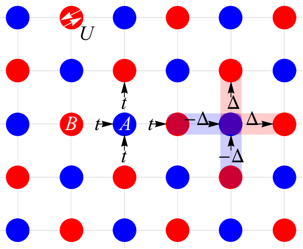
We next consider the BCS-Hubbard model on a square/cubic lattice given by $H=H_{0}+H_{int}$ stated in Ref. [Chen et al. 2018], with

where $\langle i,j\rangle$ describes nearest neighbor sites with $i\in A,j\in B$ being lattices sites belonging to different sublattices on a cubic or square lattice. $t_{ij}=t_{ji}=t$ and $\Delta_{ij}=-\Delta_{ji}=\Delta$ are hopping matrix and BCS-pairing term between sites $i$ and $j$, respectively. The last term describes on-site Hubbard interaction $U$ where $l\in A,B$, i.e. all lattices sites where $n_{l\sigma}=c^{\dagger}_{l\sigma}c_{l\sigma}$. The BCS-pairing term describes a p-wave superconductor with equal spin pairing (ESP). We shall consider a pairing term $\Delta_{ij}=\Delta$ which is positive when $i\in A,j\in B$ (see Fig. 3). Through the construction of Majorana fermions and a staggered $\mathrm{SO}(4)$ rotation corresponding to Case b of Sec. II.2, the Hamiltonian (24) can be transformed to a simple form

where $t=\tilde{t}(1+\delta)$ and $\Delta=\tilde{t}(1-\delta)$. In the limit $t=\Delta$ (or $\delta=0$), the kinetic ($H_{0}$) term is expressed in terms of Majorana fermions $\gamma$’s only. The Hamiltonian describes an extended MFKM.

The above model exhibits interesting properties. It has spin-$1/2$ chargeless quasi-particles and solitonic excitations which may be fermions or bosons, depending on the strength of interaction. The energy and spin carried by the solitonic excitation are shown in Fig. 4. The main difference between this model and the Haldane-Hubbard model described in Sec. III.1 is that here the charge excitation is always zero. This is because the quasi-particles are equal superposition of particle- and hole- excitations in the present model. Furthers details can be found in Ref. [Chen et al. 2018].

We note that an extension of this model that describes a topological superconductor has also been proposed recently by introducing a next nearest neighbor hopping and pairing in a honeycomb lattice [Ezawa 2018].

It is interesting to examine the effect of particle-hole transformation described in Sec. II.2 on this model. Consider

where $a=1,b=0$ on A-sublattice and $a=0,b=1$ on B-sublattice. In terms of $\tilde{c}$- fermions, the model becomes

Notice that the hopping term becomes an extend-$s$-wave BCS pairing term and the pairing term becomes a vector (spin triplet) hopping term under this transformation. This is not surprising since our model breaks rotation symmetry and $s-$ and $p-$ wave pairings are in general mixed in our model. Notice also that under the particle-hole transformation, the charge carried by the $c$- and $\tilde{c}$- fermions are the same on $A$-sublattice, but are opposite on $B$-sublattice. For more general particle-hole transformations, the charge carried by the $c$- fermions may be a fraction of the charge carried by the $\tilde{c}$- fermions and vice versa as we shall see in the next subsection.

In this subsection, we consider two related examples of BCS-Anderson lattice models. The models are extended MFKM’s as discussed in Sec. II.3 . The first model we consider has Hamiltonian

where $\sigma=\uparrow,\downarrow$ are spin variables . $c(c^{\dagger})$ is the annihilation (creation) operator for $c$-fermions while $f(f^{\dagger})$ is the annihilation (creation) operator for localized $f$-fermion. $\langle i,j\rangle$ denotes nearest neighbors on the lattice. $\epsilon_{\sigma}=\mu+\sigma B$ represents a spin-dependent on-site energy for $c$-fermions. The on-site energy term is set to be zero for the $f$-fermions. There is an on-site Hubbard interaction $U$ between $f$-fermions.

$H_{c}$ describes an onsite coupling between the $c$- and $f$-fermions with

in our first model. In the basis $\Psi_{c}=\{c_{\uparrow},c_{\downarrow},c_{\uparrow}^{\dagger},c_{\downarrow}^{\dagger}\}^{T}$ and $\Psi_{f}=\{f_{\uparrow},f_{\downarrow},f_{\uparrow}^{\dagger},f_{\downarrow}^{\dagger}\}^{T}$, this term is represented as $H_{c}=\sum_{i}\Psi_{ci}^{\dagger}h_{c}\Psi_{fi}$ where

In this case, the Majorana fermions $\xi_{i\sigma}=i(f_{i,\sigma}-f^{\dagger}_{i,\sigma})$ does not enter $H_{c}$ and $D_{i}=i\xi_{i\uparrow}\xi_{i\downarrow}$ is a constant of motion in the Hubbard interaction term. The model reduces to an extended MFKM. The ground state of the system is determined by the configuration of $D_{i}$’s that minimizes the total energy. We have performed the calculation numerically for a one-dimensional lattice with periodic boundary condition and find that the ground state configuration is fully determined by the relation between chemical potential $\mu$ and Zeeman field $B$. When $\mu>B$ the system favors uniform configuration $D_{i}=D\forall i$. When $B>\mu$ the system favors staggered configuration $D_{i}=(-1)^{i}D$. The uniform and staggered configurations are degenerate when $\mu=B$. The relation between $B>(<)\mu$ can be understood by making a transformation for the system

References

- Falicov and Kimball (1969) L. Falicov and J. Kimball, Phys. Rev. Lett. 22, 997 (1969).
- Ramirez et al. (1970) R. Ramirez, L. Falicov, and J. Kimball, Phys. Rev. B. 2, 3383 (1970).
- Kennedy (1994) T. Kennedy, in The State Of Matter: A Volume Dedicated to EH Lieb (World Scientific, 1994), pp. 42–80.
- Freericks and Zlatić (2003) J. Freericks and V. Zlatić, Rev. Mod. Phys. 75, 1333 (2003).
- Haller and Kennedy (2001) K. Haller and T. Kennedy, Journal of Statistical Physics 102, 15 (2001).
- Lemański et al. (2002) R. Lemański, J. K. Freericks, and G. Banach, Phys. Rev. Lett. 89, 196403 (2002).
- Lebowitz and Macris (1994) J. L. Lebowitz and N. Macris, Rev. Math. Phys. 6, 927 (1994).
- Zenker et al. (2010) B. Zenker, D. Ihle, F. X. Bronold, and H. Fehske, Phys. Rev. B 81, 115122 (2010).
- Žonda et al. (2009) M. Žonda, P. Farkašovskỳ, and H. Čenčariková, Phase Transitions 82, 19 (2009).
- Jaksch et al. (1999) D. Jaksch, H.-J. Briegel, J. I. Cirac, C. W. Gardiner, and P. Zoller, Phys. Rev. Lett. 82, 1975 (1999).
- Liu et al. (2004) W. V. Liu, F. Wilczek, and P. Zoller, Phys. Rev. A. 70, 033603 (2004).
- Mandel et al. (2003) O. Mandel, M. Greiner, A. Widera, T. Rom, T. W. Hänsch, and I. Bloch, Phys. Rev. Lett. 91, 010407 (2003).
- Yi et al. (2008) W. Yi, A. Daley, G. Pupillo, and P. Zoller, New Journal of Physics 10, 073015 (2008).
- Chen et al. (2018) Z. Chen, X. Li, and T. K. Ng, Phys. Rev. Lett. 120, 046401 (2018).
- Prosko et al. (2017) C. Prosko, S.-P. Lee, and J. Maciejko, Phys. Rev. B 96, 205104 (2017).
- Majorana (1937) E. Majorana, Il Nuovo Cimento (1924-1942) 14, 171 (1937).
- Xu and Sachdev (2010) C. Xu and S. Sachdev, Phys. Rev. Lett. 105, 057201 (2010).
- Anderson (1961) P. W. Anderson, Physical Review 124, 41 (1961).
- Chen and Nussinov (2008) H.-D. Chen and Z. Nussinov, Journal of Physics A: Mathematical and Theoretical 41, 075001 (2008).
- Feng et al. (2007) X.-Y. Feng, G.-M. Zhang, and T. Xiang, Phys. Rev. Lett 98, 087204 (2007).
- Kitaev (2006) A. Kitaev, Annals of Physics 321, 2 (2006).
- Miao et al. (2018) J.-J. Miao, H.-K. Jin, F.-C. Zhang, and Y. Zhou, arXiv preprint arXiv:1806.10960 (2018).
- Jotzu et al. (2014) G. Jotzu, M. Messer, R. Desbuquois, M. Lebrat, T. Uehlinger, D. Greif, and T. Esslinger, Nature 515, 237 (2014).
- Jotzu et al. (2015) G. Jotzu, M. Messer, F. Görg, D. Greif, R. Desbuquois, and T. Esslinger, Phys. Rev. Lett. 115, 073002 (2015).
- Watson and Lemanski (1995) G. Watson and R. Lemanski, Journal of Physics: Condensed Matter 7, 9521 (1995).
- Haldane (1988) F. D. M. Haldane, Phys. Rev. Lett. 61, 2015 (1988).
- Liu and Wang (2015) Y.-H. Liu and L. Wang, Phys. Rev. B 92, 235129 (2015).
- Houtappel (1950) R. M. F. Houtappel, Physica 16, 425 (1950).
- Ezawa (2018) M. Ezawa, Phys. Rev. B 97, 241113(R) (2018).
- Miao et al. (2019) J.-J. Miao, D.-H. Xu, L. Zhang, and F.-C. Zhang, arXiv preprint arXiv:1903.06101 (2019).