Self-triggered distributed -order coverage control
Abstract
A -order coverage control problem is studied where a network of agents must deploy over a desired area. The objective is to deploy all the agents in a decentralized manner such that a certain coverage performance metric of the network is maximized. Unlike many prior works that consider multi-agent deployment, we explicitly consider applications where more than one agent may be required to service an event that randomly occurs anywhere in the domain. The proposed method ensures the distributed agents autonomously cover the area while simultaneously relaxing the requirement of constant communication among the agents. In order to achieve the stated goals, a self-triggered coordination method is developed that both determines how agents should move without having to continuously acquire information from other agents, as well as exactly when to communicate and acquire new information. Through analysis, the proposed strategy is shown to provide asymptotic convergence similar to that of continuous or periodic methods. Simulation results demonstrate that the proposed method can reduce the number of messages exchanged as well as the amount of communication power necessary to accomplish the deployment task.
I Introduction
This paper studies a multi-agent coordination problem where a network of agents perform a deployment task to statically position themselves over a desired area. For example, a mobile sensor network where it is required to deploy sensors to positions that will maximize total coverage of the desired sensing environment. This is commonly referred to as coverage control. Specific applications include topics such as environmental monitoring [1, 2], survelliance [3], data collection [4, 5], and search and rescue [6]. More specifically, we consider a generalization of the coverage problem that extends to scenarios where more than one agent may be required to overlap a region in the coverage area. This is referred to as -order coverage control [7, 8, 9], where agents must overlap coverage of the same point . Our contributions focus on the development of coordination strategies that will reduce the amount of communication necessary between agents while performing the deployment task. This is accomplished by the design of a self-triggered algorithm where agents autonomously decide when they require information from other agents in the network.
With respect to coverage control, the majority of previous research has focused on scenerios where an individual agent is capable of servicing events that occur in the agent’s respective region of responsibility without the assistance of other agents. As an example, consider a monitoring application where a wirless sensor network must monitor the environment. If a random event occurs in the vicinity of a particular sensor then that sensor has the ability to measure and capture the event independent of other sensors in the network. However, various applications exists where agents do not possess the capability to capture or respond to events independently. These applications require multiple agents to work collectively in order to service events. One example of this type of application is that of Time Difference of Arrival (TDOA) localization [10, 11, 12] where the requirement is that three or more sensors that are located at different positions must measure the same event. Another example is emergency response vehicles where two or more vehicles may be required to respond to a particular event, such as a fire or burglary. In other scenarios, two or more agents may not be necessary for event handling, but the application may require redundant agents to overlap areas for fail-safe purposes.
Literature review
The topic of multi-agent coverage control has been studied by a number of authors in the past including the seminal work [13] where coverage control based on agents moving to the centroids of a Voronoi partition was introduced. In [14], the authors consider the coverage control problem where each node is constrained to have neighboring nodes. The authors use an approach based on vector potential fields where each node acts as a repelling force in order to maximize coverage and acts as an attracting force in order to satisfy the neighbor constraint. In [15], the authors consider heterogeneous and non-point source nodes as well as non-convex enviroments. In [16], the authors study the problem in the context of using sensor measurements to estimate regions of importance in the mission space thus driving nodes to concentrate in these areas. Common to all the above mentioned works is the fact that they study the coverage control problem in terms of a first-order coverage problem where each agent is solely responsible for covering a sub-region of the mission space. As previously mentioned, the interest of our work is the generalized -order coverage control problem where multiple agents overlap coverage of sub-regions in the mission space.
The -order coverage control problem was studied in [17, 18, 19] where a method using higher-order Voronoi partitions was proposed. The authors present a method for deploying agents over a bounded area when more than one agent must have overlapping coverage of the same point. However, to realize the proposed contol law in [19], it is assumed that continuous communication between agents is achievable. For many real-world systems, continuous communication is not feasible and periodic solutions can be resource inefficient and may not be neccessary. As alternatives to continuous and periodic solutions, self-triggered and event-triggered approaches have been proposed in the literature to handle similiar problems in networked systems [20, 21, 22, 23, 8]. For self- and event-triggered solutions, the exact time at which agents perform actions, e.g. wirelessly communicate or update a control signal, is autonomously decided by the agents rather than occurring at periodic time intervals.
In [24, 25], the concepts of self-triggered control was applied to the case of first-order optimal deployment. In our current work, we extend the self-triggered centroid algorithm presented in [24] by considering the higher-order coverage control problem studied in [17, 18, 19] and develop a self-triggered coordination strategy to relax the synchronous, periodic communication requirement while guaranteeing that each agent moves such that it does not contribute negatively to the task.
Statement of contributions
The main contribution of this work is the development of a distributed self-triggered control strategy that deploys a set of agents to static locations in a convex area in order to achieve -order optimal coverage. Our solution relaxes the need for continuous or periodic communication among agents as is done in prior works [19]. More specifically, our algorithm is comprised of two major sub-components. The first being an update decision policy where each agent decides when to acquire new information from neighboring agents through a wireless communication network. The decision to comunicate is based on the level of uncertainty each agent has accumulated over time. This uncertainty is due to not having up-to-date information that results from the lack of communication with other agents. We extend the notion of uncertain spatial partitioning [26, 27, 28] used for optimal deployment in [24] by the use of -order guaranteed and dual-guaranteed Voronoi partitions. The second major sub-component is a motion control law that determines how agents should move given possibly outdated information about the location of other agents in the network. Each agent determines a motion plan that is guaranteed to contribute positively to the higher-order deployment task.
Organization
Section II outlines some important notions from computational geometry. Section III formally presents the problem statement. Section IV formulates the concepts of -order guaranteed and -order dual-guaranteed Voronoi partitions. Section V presents the algorithm design. In section VI convergence analysis of the algorithm is discussed. Section VII presents simulation results and section VIII assimilates the conclusions.
II Preliminaries
Let and be the set of non-negative real, integer values respectively. With the Euclidean norm defined by
II-A Basic geometric notions
We denote by the closed segment with extreme points and . Let be a bounded measurable function that we term density. For , the mass and center of mass of with respect to are
Let be subsets of and be a partition of then mass and center of mass with respect to and the partitions,
The circumcenter of a bounded set is the center of a closed ball of minimum radius that contains . The circumradius of is the radius of this ball. The diameter of is .
Given , let be the unit vector in the direction of . Given a convex set and , let denote the orthogonal projection of onto , i.e., is the point in closest to . The to-ball-boundary map takes to
Figure 1 illustrates the action of .
We denote by the closed ball centered at with radius and by the closed halfspace determined by that contains .
II-B 1-order Voronoi partitions
The methods developed in this work rely heavily on the concept of Voronoi partitioning [29]. In the following sub-sections a brief discussion of 1-order Voronoi partitions is presented. Let be a convex polygon in and be the location of agents. A partition of is a collection of polygons with disjoint interiors whose union is . The Voronoi partition of generated by the points is
Intuitively, the Voronoi cell represents all the points that are closer to the agent at position than to any of the other agents in the network. When the Voronoi regions and are adjacent (i.e., they share an edge), is called a (Voronoi) neighbor of (and vice versa). is a centroidal Voronoi configuration if it satisfies that , for all .
III Problem statement
III-A k-order Voronoi partitions


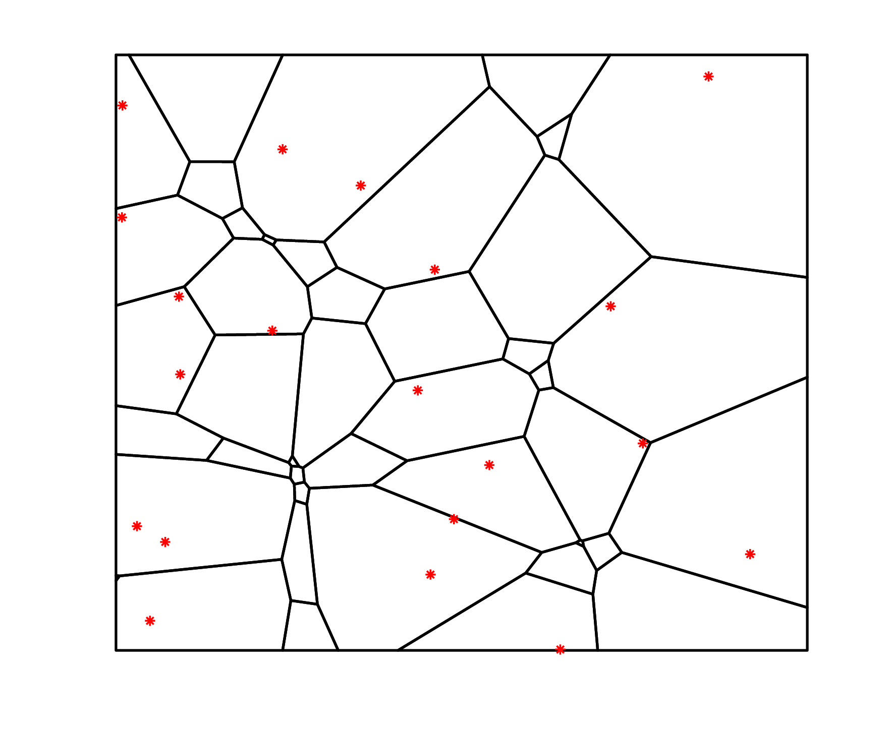
Intuitively, a -order Voronoi cell represents all the points that are closer to agents located at positions than to any of the other agents in the network. A -order Voronoi partition would then be a collection of all the -order Voronoi cells. In the first-order case, the space is partitioned into cells such that each agent is closest to every point in their cell than any of the other agents. However, in the case of a second-order partition the space is partitioned into cells and there are many cells that can be empty because certain agents may not share overlapping responsibility for any points in the space. The difference between the first-order and second-order case can be seen in figure 2. In figure 2a an example of a first-order partition is illustrated for five agents. Note that each agent is enclosed in their respective cells and there is exactly five cells, one per agent. Figure 2b illustrates the second-order partition for the same five agents. Note that in figure 2b the number of cells are greater than the number of agents. Also note that some cells contain multiple agents while other cells do not contain any agents at all. Furthermore, some agent combinations are not associated to a cell at all, e.g. and . This is due to the fact that these agents do not share points in the space that are mutually closer to them combined than to any of the other agents. A more formal definition of the -order Voronoi partition follows.
Let be a convex polygon in a -dimensional space. Let be a finite set of integers representing the agents in a -agent network. Let be the set of positions of the agents in the domain . Let be a -tuple element of the set where is the set of -tuples in that do not repeat, for example , but . Let be the subset of agent positions corresponding to the agents . The collection of all elements that include a particular agent is denoted by where A -order partition of is a collection of polygons with disjoint interiors whose union is and where an element in is associated with -agents.
The -order Voronoi partition of a convex polygon can be defined as follows. Given a set of agents with positions . For , let with . Then the -order Voronoi region associated with agents with generating sites is defined as
For example, if then and the second-order Voronoi cell for agents becomes,
For every point in , the distance from to any agent position in is less than or at most equal to the distance from to all other agent positions not in . For , the second-order Voronoi partition with and would mean that the two agents and are closer to or at most as close to all the points in than any of the other agents . An alternative interpretation would be that the agents and are considered responsible for the region defined by .
Combining all -order Voronoi regions in , the -order Voronoi partition of the environment becomes . The environment can be considered as the union of all -order Voronoi cells . Figure 2 presents an example of the difference between a first-order (2a) and second-order (2b) Voronoi partition for five agents. For any agent with position , there can be multiple sets that contain meaning that an agent located at position can be responsible for multiple -order Voronoi cells. The collection of -order Voronoi cells associated with agent is given by . All -order cells associated with agent can be combined to form a single region of that agent is responsible for and this cell is referred to as the dominant region of agent . The dominant region for agent is be defined by
The dominant cell represents the region of that agent is responsible for covering. Note that the first-order cell and the -order cell are not equivalent, but both are convex. However, the dominant cell may not be convex. The -order neighbors of agent is denoted by . For a -order Voronoi partition, is a centroidal - order Voronoi configuration if it satisfies , for all . Next, optimal deployment for -order Voronoi partitioning is discussed.
III-B Objective for higher-order coverage
The interest is in applications where agents are required to service an event occuring at a random point . This is in contrast to the 1-order problem where for any point only one agent is responsible. In order to optimally deploy agents throughout the mission space, an objective function for the higher order deployment problem must be defined. For the 1-order case, from [13], the objective function in terms of Voronoi partitions is defined as
| (1) |
The objective here is to minimize the distance from agent ’s position to all points . Taking advantage of the parallel axis theorem, may be expressed as,
| (2) |
where is the polar moment of inertia of the 1-order Voronoi cell centered at the centroid . Taking the partial derivative of (2) with respect to and evaluating at zero will produce the minimum at position for agent . The partial derivative of (2) with respect to is given by,
This demonstrates that the objective function in the 1-order case is minimal when is located at the centroid .
For Voronoi partitions of the -order, a similar approach to the order- partition can be followed. In [19] an objective function for higher-order coverage control with a general performance measure was introduced and a detailed derivation with performance measured defined by Euclidean distance for was presented. For completeness, the objective function is restated for arbitrary . The objective function in terms of a -order partition of is defined as,
| (3) |
Where is the performance measure given by,
The objective function in terms of -order Voronoi partitions is defined as,
| (4) | ||||
Unlike like the first-order Voronoi objective function where the integration occurred over each cell and there was a cell for each agent, the -order case does not have a one-to-one relationship between cells and agents. The performance measure is based on the distance -agents are from each point in . However, by manipulation, the objective function can be written in terms of the contribution of each agent separately. By distributing the integral,
and summing over all cells for each agent,
the higher-order objective function can be expressed in terms of the polar moment of inertia,
| (5) | ||||
From (5), it can be seen that the value of depends on the distance from an agent to the centroid of a given cell. Clearly an agent cannot be located at the centroid of all the cells it is responsible for. To solve for the optimal location for agents to be located, the function is described in matrix form as follows,
Where is a vector of ones, is a diagonal matrix, is a vector of cell centroids associated with agent , and is a diagonal matrix with elements on the diagonal represent the mass of the respective cell. Now the the optimal position for agent can be solved by,
is the centroid of the dominant cell . As mentioned in the previous section, the cell is the dominant cell of agent , which is the union of all the -order Voronoi cells associated with agent . The objective function is minimal when is located at the centroid of the dominant cell . This leads to the following lemma.
Lemma III.1
Given and a k-order partition of ,
i.e., the optimal partition is the -order Voronoi partition. For with , ,
i.e., the optimal positions of agents are the centroids.
As discussed in [19], for continuous control and communication the gradient descent control law is given by for gain . However, implementing this in continuous time assumes that agents have exact position information about their neighbors at all times. Instead, we next discuss how to relax this requirement without resorting to a synchronous, periodic implementation.
III-C Communication between agents
We assume agent has access to its own position at all times , but must communicate with neighbors to obtain their positions . Similar to [24], a request-response communication model is used where agent is able to request position from agent and agent immediately responds with this information. We assume that packet loss does not occur and that round-trip latency is negligible such that agent can request and receive information instantaneously i.e. the action of requesting and responding information occurs within the same timestamp.
More specifically, let be the sequence of times at which agent requests information from some neighbor . Then, agent only has access to the position of agent at these times, e.g., at timestep agent has access to .
III-D Agent state representation
If an agent does not request information on every timestep then that agent does not have access to the current position of other agents. Therefore, agent maintains state information pertaining to the most recent known position of agent in addition to information that is able to model the evolution of uncertainty over time that exists with respect to agent ’s current position. Given that agent has acquired position from agent at timestep , let be the amount of time that has elapsed since agent has communicated with agent . Then the position where will be unknown to agent at time . However, if the maximum speed for agent is known then agent can determine the set of all possible positions where agent could have traveled to in time duration . The set of possible positions for agent can be represented by a closed ball with center at and radius . To maintain state, each agent stores and in memory for every agent in the network. The data storage for agent is then defined by,
| (6) |
where for all time since it is assumed that agent always has access to it’s own position at every timestep. There exists two methods for which the contents of the data structure may be updated. The first is a time evolution update where all values increase in magnitude based on the the time duration . The second update method, referred to as the information/position update, corresponds to the acquisition of a new position value via means of communication with agent . When a position update occurs for , the value is reset i.e. . This is due to the fact that the exact position of agent is known at the instance in time that has been received and stored in memory by agent . In addition, two explicit methods for agent to extract information from . The first is the map that allows agent to extract position information from . The second extraction map , where , allows agent to extract a subset from data storage.
III-E Agent dynamics
Considering the set of agents moving in a convex polygon with positions . We consider discrete-time, single-integrator dynamics
| (7) |
where denotes the length of time of one timestep, and denotes the input at timestep with for each agent . The interest is in optimally deploying these agents in the domain such that agents overlap responsibility for every point . Equipped with a communication model, a state data model, and agent dynamics the formal problem may now be presented by the following,
Problem III.2
Given a set of agents moving in a convex polygon with dynamics (7), maximum speed , spatial density , and only depending on information local to agent , find a distributed communication and control strategy such that .
Based on the data that each agent stores in memory, the exact computation of the -order Voronoi cell cannot necessarily be achieved at each timestep. Next we address the issue of space partitioning with uncertainty for general cases of -order.
IV Space partition with uncertain information
If agent does not have access to the exact location of agent , then the uncertain position of agent with respect to agent can be represented to be within a set of points . This set represents all the possible points where agent is guaranteed to be located relative to agent . The consequence of this representation is that agent cannot compute it’s dominant region exactly. However, because the position of agent is guaranteed to be constrained to the set , it is possible for agent to compute regions in that pertain to a) the points that are certain to be part of its dominant cell, b) the points that are certain not to be part of agent ’s dominant cell, and c) the region where it is uncertain if the points belong to agent ’s dominant cell or not. The region of points that are certain to be part of agent ’s dominant cell is referred to as the -order guaranteed dominant cell of agent . The region of points that are certain to not be a part of agent ’s dominant cell is referred to as the -order dual-guaranteed dominant cell. Similar to the case of certain sites, we construct the guaranteed and dual-guaranteed dominant cell of an agent by means of the -order guaranteed and dual-guaranteed Voronoi cells. The the -order guaranteed Voronoi partition is described next.
IV-A k-order guaranteed Voronoi partitions


To assist in the exposition that follows, the first-order guaranteed Voronoi cell is briefly mentioned. The first-order guaranteed Voronoi cell for agent is given by,
The cell contains the points of that are guaranteed to be closer to than to any other , with . The uncertain regions and are considered to be closed balls ) and ) centered at and with radius and , respectively. The set is the collection of uncertain regions for agents. Similar to the discussion of -order Voronoi partitions of certain sites where and , a subset of is defined by Given and with , the -order guaranteed Voronoi cell associated with agents is defined by,
The -order guaranteed Voronoi cell represents the points that are guaranteed to be closer to the -agents in with positions in than to the agents with positions in . For example, with the -agents becomes and has positions such that the second-order guaranteed Voronoi cell associated with agents and is given by,
with . For agent , the guaranteed dominant region can be defined by,
The cell represents the region that agent is guaranteed to be responsible for covering.
IV-B k-order dual-guaranteed Voronoi partitions


In [24], the concept of dual-guaranteed Voronoi partitions was presented. Here we extend this concept to the case of -order dual-guaranteed Voronoi partitions. Again using and , the -order dual-guaranteed Voronoi cell for agents in is defined by,
The region outside of the cell represents the points that are guaranteed to be closer to agents in than to the agents in . The dual-guaranteed dominant region associated with agent is given by,
The region outside of cell represents the points that agent is guaranteed not to be responsible for covering.
Next, a solution that includes both the design of a motion control law and a communication strategy for the above stated problem is presented.
V Self-triggered higher order coverage optimization
Given the problem described in Section III, one possible approach would be for agent to periodically acquire position information from other agents. This would occur at each time step where agent would 1) acquire new information, 2) Compute it’s dominant cell , 3) compute the centroid , 4) move towards at , 5) repeat. However, similar to continuous communication, a periodic method requires frequent communication and a potentially unnecessary computational burden. The method proposed in the following section attempt to alleviate the communication and computational burden by a two part approach. The first component is a motion control law to determine how agents move when the information they possess is not up to date with respect to the most recent time step. The second component is an information update policy that allows each agent to decide when information from other agents should be acquired.
V-A Motion control
If agent has access to the exact positions of other agents then agent is capable of computing the exact dominant cell . Consequently, agent can compute the centroid . Once has been computed, agent may simply move towards it. When agent does not communicate with the other agents in the network, the exact location of the other agents will be unknown to agent . Since the exact locations of other agents is unknown, each agent must rely on the data that it does possess as a means for deciding how to move. The data that an agent does possess at any given time step includes the most recent position update that it has received from the other agents and the time that has elapsed since the last update.
Informally, the motion control law is described by the following. At each time step each agent uses the information that it has stored to compute it’s -order guaranteed and dual-guaranteed Voronoi cells. Next, each agent computes it’s guaranteed and dual-guaranteed dominant cells. Once the agent has computed these cells, the agent then computes the centroid for the guaranteed dominant cell and begins moving toward it.
The motion control law assumes that each agent has access to the value of the density over it’s -order guaranteed dominant cell. The motion control law as describe above does not necessarily guarantee that agents will move closer to the centroids of their dominant cells without applying additional constraints on agent movement. As in [24], the following lemma applies.
Lemma V.1
Given , let such that , then .
Following lemma V.1, if is the position of agent that is moving toward in the direction of the computed goal then the distance to decreases while
| (8) |
holds. Since is unknown to agent the right hand side of 8 cannot be computed. However the value can be bounded such that
| (9) |
where is given by
| (10) |
Therefore, agent moves towards as much as possible in one timestep while maintaining the condition in (9). The motion control law is formally defined in table (1).
For every consecutive time step that an agent goes without receiving updated information, (10) increases making the condition of (9) less likely to be achievable. Leading to the condition where the agent can no longer move in a manner that does not increase the distance to . Therefore, a decision mechanism that governs when an agents will acquire new information is required and is discussed next.
Agent performs:
V-B Update decision policy
The second major aspect of the self-triggered deployment strategy provides a decision mechanism that determines when an agent must perform an information update via communication with other agents. Updates to position information will be necessary for an agent to reduce the level of uncertainty that it has accumulated since the last time an update occurred. As previously mentioned, as time elapses without receiving position information from other agents, the true location of will be unknown and the set of possible locations for will continue to increase in size. Based on the motion control law presented in the previous section, agent will rely on moving towards so long as condition (9) holds. If it becomes infeasible for agent to move due to condition (9) not being satisfied, then agent must perform an information update at that moment in time in order to maintain condition (9). Therefore, the update decision policy can be describe as follows. For every timestep, each agent computes their -order guaranteed and dual guaranteed dominant cells, as well as computing the bound (10). Then each agent decides whether or not to perform a position data update. Agent will decide to perform the update when the bound (10) becomes greater than or equal to . It is possible that the points and may become close to one another i.e. for .In this case, the bound (10) may not be able to become small enough such that a position update is not required. To handle this condition, the value of is clamped at so that a minimum amount of time will pass before and update will occur. The update policy is described formally in table 2.
Agent performs:
V-C The -order self-triggered centroid algorithm
A self-triggered deployment strategy can be formulated by combining the motion control law defined in Table 1 and the update decision policy from Table 2. First, it is noted that combining the two algorithms from Table 1 and Table 2 without modification would provide an event-triggered deployment strategy. The event-triggered strategy would be performed on each timestep where agent runs the update decision policy followed by running the motion control law. This requires agent to compute , , , and from Table 2 on every timestep. However, agent is in possession of all the information necessary to predict its motion trajectory up to the time in the future where occurs. The self-triggered algorithm is presented in Table 4. In addition, note that a trivial update mechanism would provide each agent with up-to-date locations for all other agents in the network i.e. using all information stored in . However, this is costly from a communications point of view. Instead, a localized algorithm is proposed that limits the number of agents that agent must acquire information from. To compute and , agent must have knowledge of only a subset of agent positions. The subset of agents used by agent can be found by first defining
where . Based on this definition we can redefine the cell by
To locally compute at the specific time when step 4: is executed, the Dominant cell computation is used. This is borrowed from [30] and presented in Algorithm 3
The Dominant cell computation is based on agent gradually increasing its communication radius until all the information required to construct its exact -order Voronoi cell has been obtained. Combining Algorithms 1-3 leads to the complete -order self-triggered centroid algorithm described in Algorithm 5.
Agent performs:
Initialization
At time step , agent performs:


VI Convergence analysis
A detailed analysis is provided in this section to demonstrate that agents following the motion and information update strategies presented thus far will generate a network configuration such that all agents converge to their centroidal positions. The asynchronous timing of information exchange that occurs during the network evolution is dependent on the the number of agents in the network, the area of the task space, and the initial agent configuration. This presents challenges when attempting to analyze the convergent properties in a similar fashion to that of the continuous-time continuous-update policy. Instead, our analysis assumes that agents move according to the motion control law given in Table (1) while considering information updates that occur randomly in time. We show that regardless of how agents share information, trajectories governed by the motion control law, in particular the constraints laid out by , will at least converge to a positively invariant set and that if the update decision policy is followed, the network will converge to the centroidal configuration. To achieve this, a set-valued map is defined that describes the evolution of the network state represented by the data storage of all agents. Then by applying the LaSalle Invariance Principal for set-valued maps, it is shown that all trajectories generated under the state evolution map provide values of the performance function that are monotonically non-increasing. It is also shown that there exist under a weakly positively invariant set that is specifically contained in the trajectories that follow the update decision policy of Table (2). Finally, we deduced that this set coincides with the centroidal network configuration in task space. This is proposed formally by the following:
Proposition VI.1
For , the agent position evolving under the self-triggered deployment algorithm from any initial network configuration in converges to the -order Voronoi centroidal configuration.
To proceed, we formally define as the sate of an agent network where is the state of agent . We define as the map that updates both the motion and uncertainty evolution in . Recall that the magnitude of increases over time when information updates do not occur. We define as a mapping of the network state into itself and it describes the information update evolution when the update decision policy from Table (2) is followed. Note that the self-triggered algorithm can be described as the composition . Let be the set-valued map that represents any possible information-update evolution. For , the th component of is described by,
Note that is an element of the domain, but is a subset of the domain and further, is one outcome in .
Given the definition of and , the full state evolution is defined by the set-valued map where . Since is closed and is continuous, the evolution map is closed. For a trajectory generated by the self-triggered algorithm and given by then,
| (11) |
Let be a map that extracts the positions from such that .
Lemma VI.2
is monotonically non-increasing along the trajectories of .
Proof.
Let and . Let and . To demonstrate that , first the -order partition is fixed. Then for each , if the condition is true then . This is due to the fact that agent strictly follows the definition of . If instead then it is true that by lemma V.1 and (10). For both cases, and furthermore, from lemma III.1, ∎
Lemma VI.3
Proof.
Let be a trajectory of (11). First, note that being bounded implies and for there exists a converging sub-sequence of such that as . In addition, the sequence is also bounded and has a converging sub-sequence where for the sequence for . Since by definition and is closed, this implies is weakly positive invariant. Since is bounded and is non-increasing along for all of , the sequence is decreasing and bounded from below and therefore convergent. Since for any there is a converging subsequence in that converges to and since is continuous, as where is a constant. ∎


Proof of Proposition VI.1
Let be an evolution of the self-triggered centroid algorithm. Define by . Note that . Since is a trajectory of , lemma VI.3 guarantees that is weakly positively invariant and belongs to for some . Next, it is shown that
| (12) |
We reason by contradiction. Assume there exists for which there is such that . By lemma III.1, V.1 and the constraint given by (8), any possible evolution from under will strictly decrease . This is in contradiction with the fact that is weakly positively invariant for .
It is also noted that for each the inequality is satisfied at , for all an by continuity, this holds for as well. That is,
| (13) |
for all and all . Now it is shown that . Consider . Since is weakly positively invariant, there exists . Note that (12) implies that We consider two cases depending on whether agents have received information in . If agent gets updated information then and consequently from (12), and the result follows. If agent does not get updated information then and . Again using the fact that is a weakly positively invariant set, there exist Reasoning repeatedly in this manner, the only case that needs to be discarded is when agent never receives updated information. In this case while monotonically increases towards . For sufficiently large , . Then (13) implies , which contradicts the fact that tends towards .
VII Simulations


In this section, simulation results for the self-triggered deployment algorithm are presented. Simulations were performed with agents moving in a area. The timestep was set to and all agents were given the same maximum velocity of m/s. Multiple simulation iterations were performed by selecting different values of and generating random initial positions for agents on each iteration. Twenty iterations were carried out for each value of . The values selected for were . To quantify the performance of the self-triggered method, the objective function , the total transmission power, and the total number of messages transmitted were computed on every timestep. As in [24], the power output model for agent is given by
where and are parameters that are dependent on the wireless medium and is the power received from agent at agent in decibel-milliwatts. Simulation results were evaluated against a benchmark case that represents a centroidal continuous information update method where agents move toward their dominant cell centroid and positions are updated on every timestep .
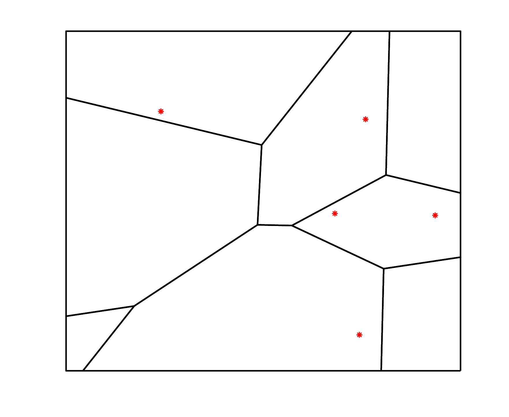
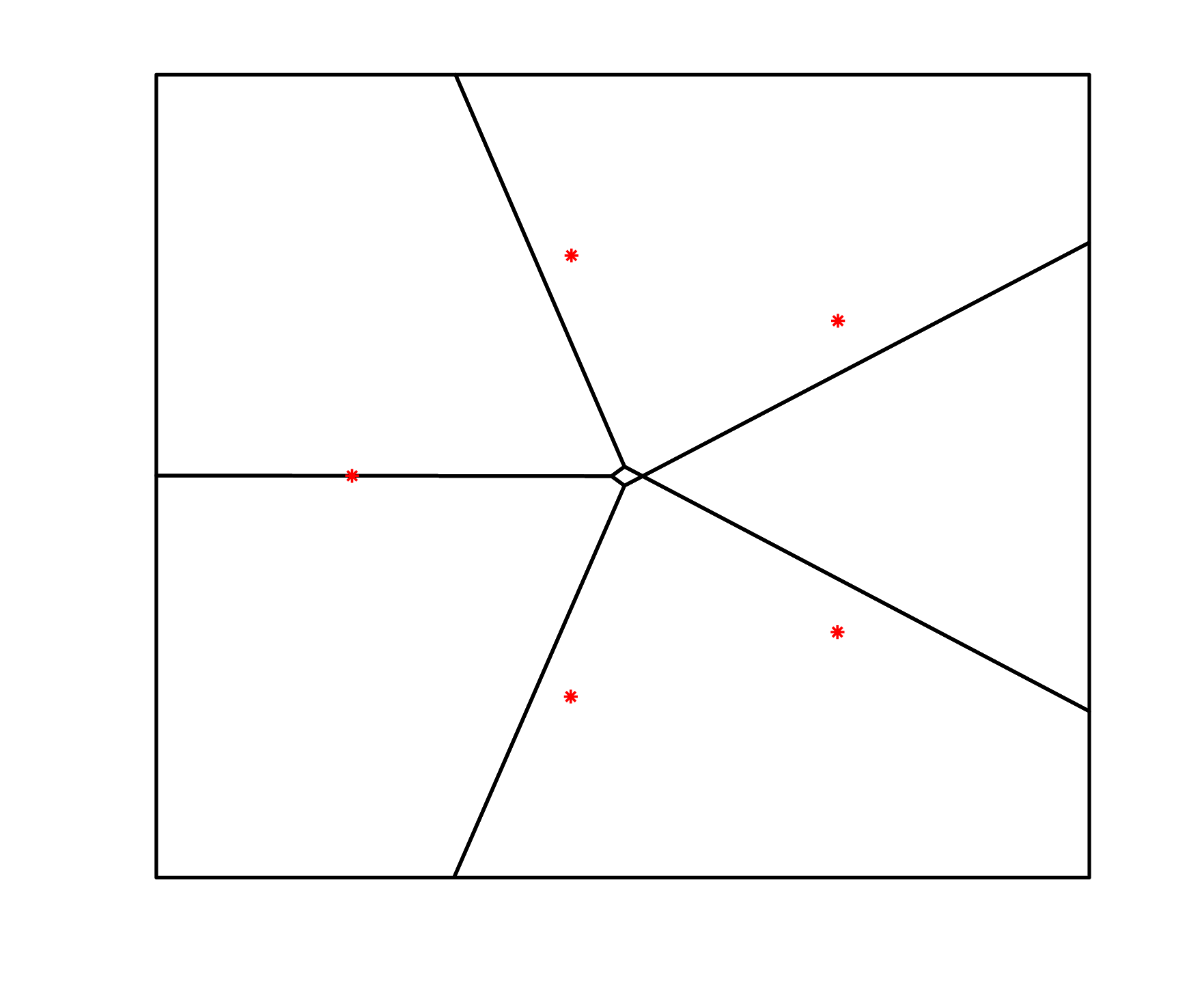
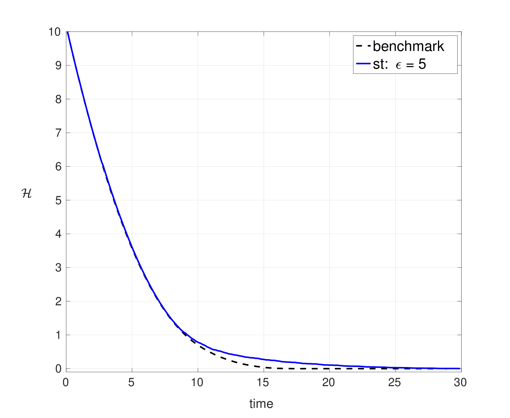
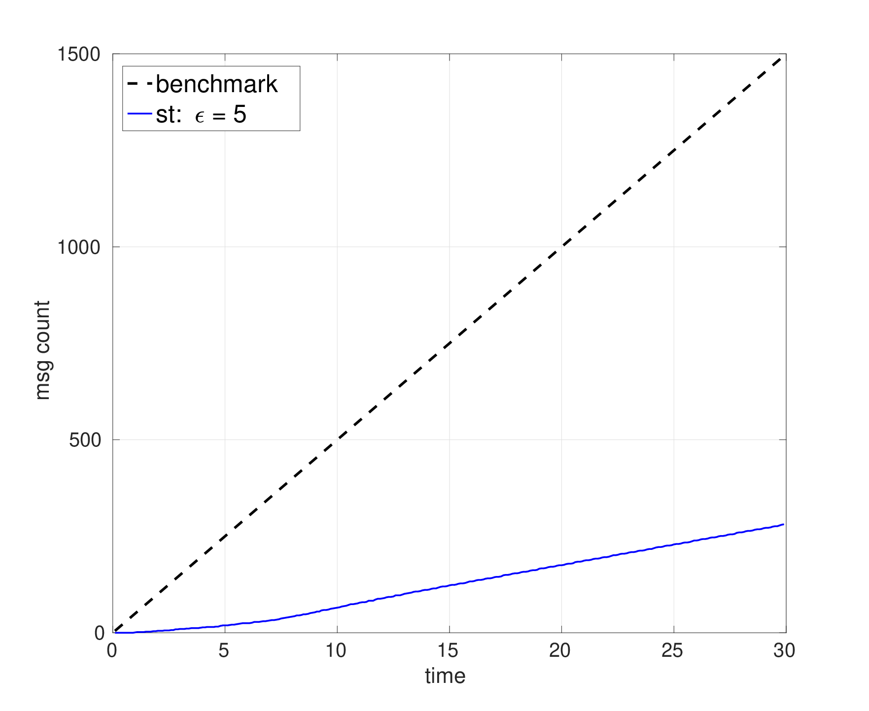
Figures 6 and 7 display the results for the execution of a single simulation instance. Figures 6 provides illustration of the initial configuration (6a), the trajectories traveled (6b), and the final configuration (6c) of all agents following the self-triggered deployment strategy. Figure (7) shows a comparison against the benchmark case of the convergence of (7a), the total message count (7b), and the communication power (7c) at each timestep. The results from figure 7 demonstrate how the self-triggered strategy can reduce both the total amount of communication and the power required to perform the deployment task. This is accomplished while still being capable of achieving convergence performance similar to that of a continuous or periodic communication strategy. Figures 8 and 9 further illustrate this point by presenting results for combined values of where twenty random initial configurations for each are averaged together. In figure 9, the value corresponds to the benchmark case. These figures illustrate how varying affects the overall performance. It can be seen that the total message count and communication power decreases when the value of increases, while the the convergence rate of degrades. However, the convergence degradation of can be considered minimal when compared to the reduction in both message count and power. For the largest value , the convergence of degrades by less than one-percent, while message count and communication power see a decrease of more than eighty-percent.
VIII Conclusions
This paper presented a -order self-triggered centroid algorithm for optimal deployment of -order coverage control scenarios. The presented strategy combined an information update policy with a motion control law. The information update policy provided a method to determine when each agent should communicate with other agents in the network. Agents communicate in order to update their data storage. The decision to communicate is based on whether an agent can continue to contribute positively to the deployment objective. The motion control law provided a method for agents to move when the locations of other agents is uncertain due to the lack of communication. Through analysis, the proposed strategy was shown to provide guaranteed asymptotic convergence. The results have shown convergence similar to that of continuous and periodic position update methods. Simulation results were able to demonstrate the potential benefits of the proposed method by illustrating the ability of the -order self-triggered centroid algorithm to not only reduce the amount of communication necessary to achieve the deployment goal, but also reducing the power consumed from communication.
References
- [1] T. B. Curtin, J. G. Bellingham, J. Catipovic, and D. Webb, “Autonomous oceanographic sampling networks,” Oceanography, vol. 6, no. 3, pp. 86–94, 1993.
- [2] Q. Lu, Q.-L. Han, B. Zhang, D. Liu, and S. Liu, “Cooperative control of mobile sensor networks for environmental monitoring: An event-triggered finite-time control scheme,” IEEE transactions on cybernetics, vol. 47, no. 12, pp. 4134–4147, 2017.
- [3] J. R. Peters, S. J. Wang, and F. Bullo, “Coverage control with anytime updates for persistent surveillance missions,” in American Control Conference (ACC), 2017. IEEE, 2017, pp. 265–270.
- [4] P. E. Rybski, N. P. Papanikolopoulos, S. A. Stoeter, D. G. Krantz, K. B. Yesin, M. Gini, R. Voyles, D. F. Hougen, B. Nelson, and M. D. Erickson, “Enlisting rangers and scouts for reconnaissance and surveillance,” IEEE Robotics & Automation Magazine, vol. 7, no. 4, pp. 14–24, 2000.
- [5] M. Zhong and C. G. Cassandras, “Distributed coverage control and data collection with mobile sensor networks,” IEEE Transactions on Automatic Control, vol. 56, no. 10, pp. 2445–2455, 2011.
- [6] A. Macwan, G. Nejat, and B. Benhabib, “Optimal deployment of robotic teams for autonomous wilderness search and rescue,” in Intelligent Robots and Systems (IROS), 2011 IEEE/RSJ International Conference on. IEEE, 2011, pp. 4544–4549.
- [7] A. Gallais and J. Carle, “An adaptive localized algorithm for multiple sensor area coverage,” in 21st International Conference on Advanced Information Networking and Applications (AINA ’07), May 2007, pp. 525–532.
- [8] J. Wang, S. Medidi, and M. Medidi, “Energy-efficient k-coverage for wireless sensor networks with variable sensing radii,” in Global Telecommunications Conference, 2009. GLOBECOM 2009. IEEE. IEEE, 2009, pp. 1–6.
- [9] J. Yu, S. Wan, X. Cheng, and D. Yu, “Coverage contribution area based -coverage for wireless sensor networks,” IEEE Transactions on Vehicular Technology, vol. 66, no. 9, pp. 8510–8523, Sep. 2017.
- [10] F. Gustafsson and F. Gunnarsson, “Positioning using time-difference of arrival measurements,” in Acoustics, Speech, and Signal Processing, 2003. Proceedings.(ICASSP’03). 2003 IEEE International Conference on, vol. 6. IEEE, 2003, pp. VI–553.
- [11] W. A. Gardner and C.-K. Chen, “Signal-selective time-difference-of-arrival estimation for passive location of man-made signal sources in highly corruptive environments. i. theory and method,” IEEE Transactions on signal processing, vol. 40, no. 5, pp. 1168–1184, 1992.
- [12] G. Mellen, M. Pachter, and J. Raquet, “Closed-form solution for determining emitter location using time difference of arrival measurements,” IEEE Transactions on Aerospace and Electronic Systems, vol. 39, no. 3, pp. 1056–1058, 2003.
- [13] J. Cortes, S. Martinez, T. Karatas, and F. Bullo, “Coverage control for mobile sensing networks,” IEEE Transactions on robotics and Automation, vol. 20, no. 2, pp. 243–255, 2004.
- [14] S. Poduri and G. S. Sukhatme, “Constrained coverage for mobile sensor networks,” in Robotics and Automation, 2004. Proceedings. ICRA’04. 2004 IEEE International Conference on, vol. 1. IEEE, 2004, pp. 165–171.
- [15] L. C. Pimenta, V. Kumar, R. C. Mesquita, and G. A. Pereira, “Sensing and coverage for a network of heterogeneous robots,” in Decision and Control, 2008. CDC 2008. 47th IEEE Conference on. IEEE, 2008, pp. 3947–3952.
- [16] M. Schwager, J.-J. Slotine, and D. Rus, “Decentralized, adaptive control for coverage with networked robots,” in Robotics and Automation, 2007 IEEE International Conference on. IEEE, 2007, pp. 3289–3294.
- [17] B. Jiang, Z. Sun, and B. D. Anderson, “Higher order voronoi based mobile coverage control,” in American Control Conference (ACC), 2015. IEEE, 2015, pp. 1457–1462.
- [18] B. Jiang, Z. Sun, B. D. O. Anderson, and C. Lageman, “Higher order mobile coverage control with application to localization,” CoRR, vol. abs/1703.02424, 2017. [Online]. Available: http://arxiv.org/abs/1703.02424
- [19] B. Jiang, Z. Sun, B. D. Anderson, and C. Lageman, “Higher order mobile coverage control with applications to clustering of discrete sets,” Automatica, vol. 102, pp. 27 – 33, 2019. [Online]. Available: http://www.sciencedirect.com/science/article/pii/S0005109818306356
- [20] W. Heemels, K. H. Johansson, and P. Tabuada, “An introduction to event-triggered and self-triggered control,” in Decision and Control (CDC), 2012 IEEE 51st Annual Conference on. IEEE, 2012, pp. 3270–3285.
- [21] D. V. Dimarogonas, E. Frazzoli, and K. H. Johansson, “Distributed self-triggered control for multi-agent systems,” in Decision and Control (CDC), 2010 49th IEEE Conference on. IEEE, 2010, pp. 6716–6721.
- [22] D. V. Dimarogonas and K. H. Johansson, “Event-triggered control for multi-agent systems,” in Decision and Control, 2009 held jointly with the 2009 28th Chinese Control Conference. CDC/CCC 2009. Proceedings of the 48th IEEE Conference on. IEEE, 2009, pp. 7131–7136.
- [23] M. Mazo and P. Tabuada, “On event-triggered and self-triggered control over sensor/actuator networks,” in Decision and Control, 2008. CDC 2008. 47th IEEE Conference on. IEEE, 2008, pp. 435–440.
- [24] C. Nowzari and J. Cortés, “Self-triggered coordination of robotic networks for optimal deployment,” Automatica, vol. 48, no. 6, pp. 1077–1087, 2012.
- [25] C. Nowzari, J. Cortés, and G. J. Pappas, “Team-triggered coordination of robotic networks for optimal deployment,” Chicago, IL, Jul. 2015, pp. 5744–5751.
- [26] W. Evans and J. Sember, “Guaranteed voronoi diagrams of uncertain sites,” in 20th Canadian Conference on Computational Geometry, 2008, pp. 207–210.
- [27] M. Jooyandeh, A. Mohades, and M. Mirzakhah, “Uncertain voronoi diagram,” Information processing letters, vol. 109, no. 13, pp. 709–712, 2009.
- [28] R. Cheng, X. Xie, M. L. Yiu, J. Chen, and L. Sun, “Uv-diagram: A voronoi diagram for uncertain data,” in Data Engineering (ICDE), 2010 IEEE 26th International Conference on. IEEE, 2010, pp. 796–807.
- [29] M. Senechal, “Spatial tessellations: Concepts and applications of voronoi diagrams,” Science, vol. 260, no. 5111, pp. 1170–1173, 1993.
- [30] F. Li, J. Luo, S. Xin, W. Wang, and Y. He, “Autonomous deployment for load balancing k-surface coverage in sensor networks,” vol. 14, no. 1, pp. 279–293, 2015.