Service Capacity Enhanced Task Offloading and Resource Allocation in Multi-Server Edge Computing Environment

Wei Du¹², Tao Lei¹, Qiang He³, Wei Liu¹², Qiwang Lei¹, Hailiang Zhao¹, Wei Wang⁴ Affiliation: ¹ Wuhan University of Technology, Wuhan, China
{whutduwei,leitao1995, wliu, leiqiwang} @whut.edu.cn, hliangzhao97@gmail.com Affiliation: ² Hubei Key Laboratory of Transportation Internet of Things, Wuhan, China Affiliation: ³ Swinburne University of Technology, Melbourne, Australia
qhe@swin.edu.au Affiliation: ⁴ East China Normal University, ShangHai, China
wwang@dase.ecnu.edu.cn

Abstract

An edge computing environment features multiple edge servers and multiple service clients. In this environment, mobile service providers can offload client-side computation tasks from service clients’ devices onto edge servers to reduce service latency and power consumption experienced by the clients. A critical issue that has yet to be properly addressed is how to allocate edge computing resources to achieve two optimization objectives: 1) minimize the service cost measured by the service latency and the power consumption experienced by service clients; and 2) maximize the service capacity measured by the number of service clients that can offload their computation tasks in the long term. This paper formulates this long-term problem as a stochastic optimization problem and solves it with an online algorithm based on Lyapunov optimization. This NP-hard problem is decomposed into three sub-problems, which are then solved with a suite of techniques. The experimental results show that our approach significantly outperforms two baseline approaches.

Index Terms:

edge computing; multi-server task offloading; service capacity enhancement; Lyapunov optimization

I Introduction

Edge computing has emerged as a new paradigm for powering applications by offering computing, storage and networking resources at the edge of the cloud [1, 2]. As illustrated on the 5G standardization roadmap, edge servers will be distributed at ultra-dense small-cell base stations (CBS) [3, 4]. In such an environment, the coverages of adjacent edge servers partially overlap to avoid blank areas not covered by any edge servers [5]. Service providers can offload client-side computation tasks from service clients’ devices onto edge servers to reduce the service cost measured by the service latency and power consumption experienced by service clients [6, 7]. This is referred to as task offloading.

The edge infrastructure provider looks at task offloading from two general perspectives. A large number of edge servers sharing service clients’ offloaded computation tasks can provide service clients with low service cost from service clients’ perspective. That is the benefit of computation loading. However, the deployment of excessive edge servers result in overly high operational cost from edge infrastructure provider’s perspective. After all, the edge infrastructure provider is interested in the overall revenue, i.e., the benefit minus the cost. The economy of scale maximizes the edge infrastructure provider’s revenue by maximizing the service capacity,i.e., the ability to serve the maximum number of service clients. To achieve a cost-effective solution, the service cost needs to be traded off to allow more service clients to be served by edge servers. Thus, how to trade off the service cost and service capacity is a critical problem in edge computing.

A lot of researchers have focused on solving the task offloading problem in a single-server edge computing environment. However, in a particular area, there are usually multiple edge servers available for offloading service clients’ computation tasks. The edge computing environment is in fact a multi-server environment. In such an environment, it is critical and challenging to optimize the utilization of edge computing resources, including computation and transmission resources, with the aim to maximize the service capacity while minimizing the service cost. Firstly, the characteristics of latency-tolerant applications, i.e., the coupling among randomly-arrived tasks, must be captured [8]. Stochastic computation partitioning strategies must be formulated to split the resources to be shared among service clients. Secondly, each service client needs to decide not only how to partition its computation tasks between its device and the edge server but also which edge server to offload its computation tasks to.

In this paper, we propose a holistic solution to computation offloading and resource allocation in multi-server edge computing environment with the aim to serve as many service clients as possible with minimum service cost. The main contributions of this paper are as follows:

•

Task offloading in such an environment is modelled as a stochastic optimization problem with multiple optimization objectives. It aims to maximize the number of service clients served with minimum service cost in the long term.
•

Based on Lyapunov optimization, the above long-term stochastic optimization problem is converted to a deterministic optimization problem within each time slot, which is then further decomposed into three sub-problems.
•

To solve the optimization problem, an online joint task offloading and resource allocation algorithm (OJTORA) powered by a suite of techniques is proposed to solve each sub-problem with low complexity.
•

Extensive experiments are conducted to evaluate OJTORA. The results show that OJTORA outperforms the baseline approaches significantly.

The remainder of this paper is organized as follows. Section II reviews related work. Section III presents the edge computing model. Section IV formulates the research problem. Section V introduces the proposed approach. Section VI experimentally evaluates the proposed approach. Section VII concludes this paper.

II Related Works

In recent years, joint task offloading and resource allocation in edge computing has attracted many researchers’ attention. Most existing work studied the problem in a single-server edge computing environment [8, 9, 10, 11]. Some researchers have considered multi-server scenarios [12, 13, 14, 15, 16, 17, 18]. The authors of [12] optimize task offloading, uplink transmission power of service clients, and computing resource allocation on edge servers to minimize task completion time and power consumption. In [13], the tradeoff between latency and power consumption was studied. The problem was formulated as computation and transmits power minimization subject to latency and reliability constraints. The authors of [14] studied how to minimize mobile power consumption through data offloading. Centralized and distributed algorithms for power allocation and transmission channel assignment were proposed. In [15], device-edge-cloud edge was investigated. A network-aware multi-user and multi-edge computation partitioning problem was formulated. Computation and radio transmission resources were allocated such that service clients’ average throughput was maximized. In [16], the shareable storage was considered, and a constant-factor approximation algorithm was proposed to decide the server placement and resource allocation. In [17], the edge task offloading control was investigated in cloud radio access network (C-RAN) environments, and a multi-stage heuristic was proposed to minimize the refusal rate for user’s task offloading requests. In [18], an online algorithm was proposed to allocate edge server’s resource over time.

In the studies of task offloading, service latency and power consumption have been commonly acknowledged as two very important optimization objectives. However, few researchers have considered service capacity, i.e., the total number of service clients served, which is a key issue from the edge infrastructure provider’s perspective in a multi-server edge computing environment[5]. In [19]. A quality-of-experience (QoE) driven LTE downlink scheduling scheme for VoIP applications was proposed to improve the service capacity with acceptable QoE for all service clients. However, they only consider single-server environments. In addition, the proposed LTE downlink scheduling scheme is specifically designed for VoIP applications and thus is not applicable to most other applications in the edge computing environment.

Our work differentiates from existing work in the following ways. First, we consider a multi-server edge computing environment. Second, our approach is applicable to most latency-tolerant applications in the edge computing environment. Third, we consider both resource allocation and task offloading. Finally, we attempt to achieve the optimization objectives in the long term.

III System Model

An example multi-server edge computing scenario is shown in Fig. 1. A service client can offload some or all of its computation tasks to one of its nearby edge servers. Let us denote the set of service clients with $\emph{U}$ , the set of edge servers with $\emph{S}$ , the connection between the ith service client and the jth edge server with $c_{i,j}=\{0,1\}$ , where $c_{i,j}=1$ indicates that the ith service client can access the jth edge server or $c_{i,j}=0$ otherwise. Let us define $G_{i}=\{j|c_{i,j}=1,j\in S\},i\in U$ , and $Z_{j}=\{i|c_{i,j}=1,i\in U\},j\in S$ . Task offloading in the edge computing environment is an ongoing process. Let us denote different time slots with $T=\{1,2,3,...\}$ and the time slot length is $\tau$ . The available bandwidth of each edge server is $\omega$ Hz and the noise power spectral density is $N_{0}$ .

Fig. 1: A multi-server edge environment

III-A Computation Task and Task Queue Model

The computation tasks running on service clients’ devices are bit-wise independent [1]. Let us denote the amount of tasks of the ith service client in the tth time slot as $A_{i}(t)$ , which are independent and identically distributed in different time slot within $[0,A_{i,max}],A_{i,max}\in\mathbb{R}^{+}$ , with the expectation $\mathbb{E}[A_{i}(t)]=\lambda_{i},\lambda_{i}\in[0,A_{i,max}],i\in U$ . As shown in Fig. 2, at the beginning of the tth time slot, the local queue length of the ith service client is $Q_{i}(t)$ . At $t$ th time slot, the amount of tasks which has arrived but not been executed locally or offloaded will be put in $Q_{i}(t)$ . Within the tth time slot, the ith service client will locally execute $D_{l,i}(t)$ tasks and will offload $D_{r,i}(t)$ tasks to an edge server, i.e., $D_{\sum,i}(t)=D_{l,i}(t)+D_{r,i}(t)$ .

\centering Q_{i}(t+1)=max\{Q_{i}(t)-D_{\sum,i}(t),0\}+A_{i}(t),i\in U.\@add@centering

(1)

As shown in Fig. 2, a service client chooses only one edge server to offload its tasks in each time slot. Thus, we maintain a virtual task queue $H_{i}(t)$ for each service client, which represents the amount of tasks offloaded but not been executed in all edge servers. In the tth time slot, let us denote the amount of tasks of the ith service client that has been offloaded but not executed by the jth edge server as $H_{i,j}(t)$ , where $H_{i}(t)=\sum_{j\in G_{i}}H_{i,j}(t)$ , the amount of tasks of the ith service client which has been executed by the edge server as $D_{s,i}(t)$ .

\centering H_{i}(t+1)=max\{H_{i}(t)-D_{s,i}(t),0\}+D_{r,i}(t),i\in U.\@add@centering

(2)

Fig. 2: The task queues of edge system

III-B Local Execution and Task Offloading Model

The ith service client’s device executes 1bit task using $L_{i}$ (cycles/bit) CPU cycles [20, 21]. The dynamic frequency and voltage scaling (DVFS) technique is used to adjust the CPU-cycle frequency of service clients’ devices [1, 8, 12]. In the tth time slot, $f_{l,i}(t)$ is the CPU-cycle frequency of the ith service client’s device.

\centering D_{l,i}(t)=\tau f_{l,i}(t)L_{i}^{-1},i\in U.\@add@centering

(3)

According to circuit theories [22, 23], the CPU power consumption of the ith service client’s device in the tth time slot is calculated as

\centering p_{l,i}(t)=k_{mod,i}f_{l,i}^{3}(t),i\in U,\@add@centering

(4)

where $k_{mod,i}$ is the effective switched capacitance of the CPU of the ith service client’s device. $f_{max,i}$ is the maximum CPU-cycle frequency of the ith service client’s device, i.e.,

\centering 0\leq f_{l,i}(t)\leq f_{max,i},i\in U.\@add@centering

(5)

In this paper, the operational frequency band of the jth edge server is divided equally into $|Z_{j}|$ which $B_{j}=\omega/|Z_{j}|$ . In the tth time slot, let us denote the fading of wireless channels between the ith service client’s device and the jth edge server as $\gamma_{i,j}(t)$ , the channel power gain from the ith service client’s device to the jth edge server as

\centering\Gamma_{i,j}(t)=\gamma_{i,j}(t)g_{0}(\frac{d_{0}}{d_{i,j}})^{\theta},i\in U,j\in S,\@add@centering

(6)

where $g_{0}$ is a constant, $\theta$ is an exponent, $d_{0}$ is the reference distance [8], and $d_{i,j}$ is the distance between the ith service client’s device and the jth edge server. The task offloading variables in the tth time slot are defined as $\textbf{X}(t)=\{x_{i,j}(t)|i\in U,j\in S\}$ , where $x_{i,j}(t)\in\{0,1\}$ , where $x_{i,j}(t)=1$ indicates that the ith service client’s device offloads its computation tasks to the jth edge server in the tth time slot.

\centering\sum_{j\in S}x_{i,j}(t)\leq 1,i\in U.\@add@centering

(7)

The transmit power of the ith service client’s device in the tth time slot is denoted by $p_{r,i}(t)$ . According to the Shannon-Hartley formula [24], the transmit rate between the ith service client’s device and the jth edge server in the tth time slot is

\centering r_{i,j}(t)=\left\{\begin{matrix}&B_{j}\log_{2}(1+\frac{\Gamma_{i,j}(t)p_{r,i}(t)}{B_{j}N_{0}}),x_{i,j}=1&\\ &0,x_{i,j}=0&\end{matrix}\right.\@add@centering

(8)

Without loss of generality, $p_{r,i}(t)$ must not exceed the maximum transmit power of the ith service client’s device.

\centering 0\leq p_{r,i}(t)\leq p_{max,i},i\in U.\@add@centering

(9)

Based on the above definitions, the number of offloading tasks of the ith service client’s device is calculated as

\centering D_{r,i}(t)=\sum_{j\in S}r_{i,j}(t)\tau,i\in U.\@add@centering

(10)

III-C Edge Server Scheduling

As shown in Fig. 2, the edge server can transfer input data to a neighboring edge server via an X2 link [25]. The amount of tasks of the ith service client’s device that have been executed by the jth edge server in the tth time slot is denoted as $D_{s,i,j}(t)$ . Then, $D_{s,i}(t)$ can be expressed as

\centering D_{s,i}(t)=\sum_{j\in S}D_{s,i,j}(t),i\in U.\@add@centering

(11)

For the jth edge server, $f_{max,j}$ is the maximum CPU-cycle frequency and $\varphi_{j}$ is the number of CPUs.

\centering\sum_{j\in S}D_{s,i,j}(t)L_{i}\leq\tau\varphi_{j}f_{max,j}.\@add@centering

(12)

IV Problem Formulation

This section first defines the service cost function and then formulates the average service capacity, i.e., the long-term average number of service clients that can offload their tasks. Finally, the optimization problem studied in this paper is formulated.

The service cost function is defined as follows:

\centering\xi_{i}(t)=\beta\xi_{i}^{latency}(t)+(1-\beta)\xi_{i}^{power}(t),i\in U,\@add@centering

(13)

where $\beta\in[0,1]$ . $\xi_{i}^{latency}(t)$ and $\xi_{i}^{power}(t)$ are the latency cost and power cost of the ith service client’s device in the tth time slot. According to Little’s Law, the average execution delay of a service client’s device is proportional to the average amount of its tasks in the edge environment.

\centering\xi_{i}^{latency}(t)=\alpha(Q_{i}(t)-D_{\sum,i})+(1-\alpha)(H_{i}(t)-D_{s,i}(t)).\@add@centering

(14)

where $\alpha\in[0,1]$ . Therefore, $\xi_{i}^{power}(t)$ is calculated as

\centering\xi_{i}^{power}(t)=p_{l,i}(t)+p_{r,i}(t),i\in U.\@add@centering

(15)

Let us denote the long-term average number of service clients that can offload their tasks as $\bar{O}$ .

\centering\bar{O}=\lim_{T\to+\infty}\frac{1}{T\cdot m}\sum_{t=0}^{T-1}\sum_{i\in U,j\in S}x_{i,j}(t).\@add@centering

(16)

Constraint (17) requires that the service clients’ task queues are stable [26].

\centering\lim_{T\to+\infty}\frac{\textbf{E}[|Q_{i}(T)|]}{T}=0,\lim_{T\to+\infty}\frac{\textbf{E}[|H_{i}(T)|]}{T}=0.\@add@centering

(17)

Let us denote the system operation at the tth time slot with $\textbf{R}(t)\triangleq\{\textbf{f}(t),\textbf{p}(t),\textbf{X}(t),\textbf{D}(t)\}$ , in which $\textbf{f}(t)\triangleq\{f_{l,i}(t)|i\in U\}$ , $\textbf{p}(t)\triangleq\{p_{r,i}(t)|i\in U\}$ , $\textbf{D}(t)\triangleq\{D_{s,j}(t)|j\in S\}$ . Accordingly, the objective functions that minimize the average service cost and maximize the average service capacity respectively are defined below as $\emph{\textbf{P}}_{1}$ together:

\begin{split}\emph{\textbf{P}}_{1}:&\min_{\{\emph{\textbf{R}}(t)\}}\lim_{T\to+\infty}\frac{1}{T}\sum_{T-1}^{0}\textbf{E}\left[\sum_{i\in U}\xi_{i}(t)\right]\\ &\max_{\{\emph{\textbf{R}}(t)\}}\bar{O}\\ &s.t.(\ref{equ5})(\ref{equ7})(\ref{equ9})(\ref{equ12})(\ref{equ17}),t\in T\end{split}

V Algorithm Design

This section introduces an online algorithm for solving the joint task offloading and resource allocation problem $\emph{\textbf{P}}_{1}$ . Based on Lyapunov optimization, the stochastic optimization problem is converted into a deterministic optimization problem.

V-A Lyapunov Optimization-based Online Algorithm

We employ the Lyapunov optimization to ensure the stability of the task queues through minimizing the average service cost. To model the problem as a Lyapunov optimization problem, we define the Lyapunov function as:

\centering L(\bm{\Theta}(t))=\frac{1}{2}\sum_{i\in U}[Q_{i}^{2}(t)+H_{i}^{2}(t)].\@add@centering

(18)

where $\bm{\Theta}(t)=[\textbf{Q}(t),\textbf{H}(t)]$ . Then, the conditional Lyapunov drift is defined as

\centering\Delta(\bm{\Theta}(t))=\textbf{E}[(L(\bm{\Theta}(t+1))-L(\bm{\Theta}(t)))|\bm{\Theta}(t)].\@add@centering

(19)

The Lyapunov drift-plus-penalty function is defined as:

\centering\Delta_{\nu}(\bm{\Theta}(t))=\Delta(\bm{\Theta}(t))+V\cdot\textbf{E}[\bm{\xi}(t)|\bm{\Theta}(t)],\@add@centering

(20)

where $\bm{\xi}(t)=\sum_{i\in U}\xi_{i}(t)$ and $V\in(0,+\infty)$ is a control parameter to keep the balance between task queues and service cost.

The upper bound of $\Delta(\bm{\Theta}(t))$ with constraints (5), (7),
(9) and (12) is defined as:

\centering\begin{split}\Delta_{\nu}(t)\leq&C-\textbf{E}[\sum_{i\in U}Q_{i}(t)(D_{\sum,i}(t)-A_{i}(t))|\bm{\Theta}(t)]\\ &-\textbf{E}[\sum_{i\in U}H_{i}(t)(D_{s,i}(t)-D_{r,i}(t))|\bm{\Theta}(t)]\\ &+V\cdot\textbf{E}[\bm{\xi}(t)|\bm{\Theta}(t)],\end{split}\@add@centering

(21)

where $\emph{C}$ is a constant [8].

According to Lyapunov optimization, in order to minimize $\bm{\xi}(t)$ and maintain the stability of service clients’ task queues, we need to minimize the upper bound of $\Delta_{\nu}(t)$ in each time slot as expressed in formula (21). This minimization is denoted as $\emph{\textbf{P}}_{\textbf{PTS}}$ . All the constraints of $\emph{\textbf{P}}_{1}$ except constraint (17) are included in $\emph{\textbf{P}}_{\textbf{PTS}}$ . Algorithm 1 presents the pseudo code of the Online Joint Task Offloading and Resource Allocation Algorithm (OJTORA). The pseudo-code for solving $\emph{\textbf{SP}}_{1}$ , $\emph{\textbf{SP}}_{2}$ and $\emph{\textbf{SP}}_{3}$ are presented below in Section V-B.

Algorithm 1 Online Joint Task Offloading and Resource Allocation (OJTORA)

1: At the beginning of the tth time slot, the

\{\Gamma_{i,j}(t)\}

and

\{A_{i}(t)\}

will be given.

2: Get optimal

\textbf{f}(t),\textbf{p}(t),\textbf{X}(t)and\textbf{D}(t)

by solving

\begin{split}\emph{\textbf{P}}_{PTS}:&\min_{\textbf{R}(t)}-\sum_{i\in U}Q_{i}(t)D_{\sum,i}(t)\\ &-\sum_{i\in U}H_{i}(t)(D_{s,i}(t)-D_{r,i}(t))+V\cdotp\bm{\xi}(t)\\ &s.t.(\ref{equ5})(\ref{equ7})(\ref{equ9})(\ref{equ12})\end{split}

in which the optimal

\textbf{f}(t),\textbf{p}(t),\textbf{X}(t)and\textbf{D}(t)

can be obtained by solving

\emph{\textbf{SP}}_{1}

\emph{\textbf{SP}}_{2}

and

\emph{\textbf{SP}}_{3}

, respectively.

3: According to the iteration formula in (1) and (2), update the

\{Q_{i}(t)\}

and

\{H_{i}(t)\}

4: Go to the next time slot, which

t=t+1

V-B Optimal Solution to $\textbf{P}_{PTS}$

V-B1 Optimal CPU-Cycle Frequencies of Mobile Devices

The $\textbf{SP}_{1}$ is defined as

\begin{split}\textbf{\emph{SP}}_{1}:&\min_{\{\textbf{\emph{f}}(t)\}}\sum_{i\in U}[-(Q_{i}(t)+V\cdot\alpha\beta)\tau L_{i}^{-1}f_{l,i}(t)\\ &+V\cdot(1-\beta)k_{mod,i}f_{l,i}^{3}(t)]\\ &s.t.(\ref{equ5}).\end{split}

The objective function of $\textbf{\emph{SP}}_{1}$ is convex and constraint (5) is linear. Therefore, $\textbf{\emph{SP}}_{1}$ is a convex problem. For each service client, we can find that $f_{l,i}(t)$ is independent. Let us denote the optimal CPU-cycle frequency of the ith service client’s device as $f_{l,i}^{*}(t)$ . We can obtain $f_{l,i}^{*}(t)$ by finding the minimum point of $-(Q_{i}(t)+V\cdot\alpha\beta)\tau L_{i}^{-1}f_{l,i}(t)+V\cdot(1-\beta)k_{mod,i}f_{l,i}^{3}(t)$ . At the same time, $f_{l,i}^{*}(t)$ must fulfil constraint (5).

\centering f_{l,i}^{*}(t)=\left\{\begin{matrix}&min\{\sqrt{\frac{(Q_{i}(t)+V\cdot\alpha\beta)\tau}{3k_{mod,i}V(1-\beta)L_{i})}},f_{max,i}\},others&\\ &f_{max,i},\beta=1&\end{matrix}\right.\@add@centering

(22)

V-B2 Optimal Transmit Power Consumption and Task Offloading Policy

$p_{r,i}^{*}(t)$ and $\textbf{X}^{*}(t)$ refer to the optimal $p_{r,i}(t)$ and the optimal $\textbf{X}(t)$ respectively. They are obtained by solving $\textbf{SP}_{2}$ :

\begin{split}\textbf{\emph{SP}}_{2}:&\min_{\{\textbf{p}(t),\textbf{X}(t)\}}\sum_{i\in U}[-\Psi_{i}(t)D_{r,i}(t)+V(1-\beta)p_{r,i}(t)]\\ &s.t.(\ref{equ7})(\ref{equ9}).\end{split}

When there is $\Psi_{i}(t)=Q_{i}(t)-H_{i}(t)+V\cdot\alpha\beta\leq 0$ , the object function of $\textbf{SP}_{2}$ is non-decreasing with $p_{r,i}(t)$ . Then, because of constraint (9), $p_{r,i}^{*}(t)=0$ means that the ith service client’s device will not offload its tasks to edge servers. Let us denote $U_{off}(t)=\{i|\Psi_{i}(t)\geq 0,i\in U\}$ . The optimal transmit power consumption and the optimal task offloading policy can be achieved by solving $\textbf{SP}_{2}^{{}^{\prime}}$ :

\begin{split}\textbf{\emph{SP}}_{2}^{{}^{\prime}}:&\min_{\{\textbf{p}(t),\textbf{X}(t)\}}\sum_{i\in U_{off}(t)}[-\Psi_{i}(t)D_{r,i}(t)+V(1-\beta)p_{r,i}(t)]\\ &s.t.(\ref{equ7})(\ref{equ9}).\end{split}

This objective function is determined by two variables, i.e., $\textbf{p}(t)$ and $\textbf{X}(t)$ . It is hard to obtain $p_{r,i}^{*}(t)$ and $\textbf{X}^{*}(t)$ simultaneously. Therefore, we divide $\textbf{SP}_{2}^{{}^{\prime}}$ into two sub-problems.

First, we assume a $\textbf{X}^{*}(t)$ . For a fixed computation offloading policy, we denote the first sub-problem of $\textbf{SP}_{2}^{{}^{\prime}}$ as $\textbf{SP}_{PWR}$ , which can be expressed as

\begin{split}\textbf{\emph{SP}}_{PWR}:&\min_{\{\textbf{p}(t)\}}\sum_{i\in U_{off}(t)}[-\Psi_{i}(t)D_{r,i}(t)+V(1-\beta)p_{r,i}(t)]\\ &s.t.(\ref{equ9})\end{split}

where $D_{r,i}(t)$ is non-decreasing with $p_{r,i}(t)$ . The objective function of $\textbf{SP}_{PWR}$ is convex and constraint (9) is linear. Therefore, $\textbf{SP}_{PWR}$ is a convex problem. Similar to $\textbf{SP}_{1}$ , $\textbf{SP}_{PWR}$ can be decomposed for individual mobile devices. Let us denote the edge server to which the ith service client offloads its computation tasks in the tth time slot as $j^{*}$ , there is $x_{i,j^{*}}=1$ . In addition, $r_{i,j^{*}}(t)$ can be obtained by

\centering r_{i,j^{*}}(t)=B_{j^{*}}\log_{2}(1+\frac{\Gamma_{i,j^{*}}(t)p_{r,i}(t)}{B_{j^{*}}N_{0}}),\@add@centering

(23)

where $r_{i,j}(t)=0$ if $j\neq j^{*}$ . Then, $D_{r,i}(t)=r_{i,j^{*}}(t)\tau$ . Therefore, we can obtain $p_{l,i}^{*}(t)$ by finding the minimum of $-\Psi_{i}(t)D_{r,i}(t)+V\cdot(1-\beta)p_{r,i}(t)$ . Let us denote $\Lambda_{i}(t)=\frac{\Psi_{i}(t)\tau B_{j^{*}}}{V\cdot(1-\beta)\ln 2}-\frac{N_{0}B_{j^{*}}}{\Gamma_{i,j^{*}}(t)}$ . Then, the $p_{l,i}^{*}(t)$ can be written as

\centering p_{l,i}^{*}(t)=\left\{\begin{matrix}&min\{\Lambda_{i}(t),p_{max,i}\},others&\\ &p_{max,i},\beta=1&\end{matrix}\right.\@add@centering

(24)

Secondly, we assume a fixed $p^{*}(t)$ and denote the second sub-problem of $\textbf{SP}_{2}^{{}^{\prime}}$ as $\textbf{SP}_{CO}$ , expressed as follows:

\begin{split}\textbf{\emph{SP}}_{CO}:&\min_{\{\textbf{X}(t)\}}\sum_{i\in U_{off}(t)}[-\Psi_{i}(t)D_{r,i}(t)]\\ &s.t.(\ref{equ7}).\end{split}

For a service client where $i\in U_{off}(t)$ , it independently selects an edge server to offload its computation tasks. Therefore, $\textbf{SP}_{CO}$ can be decomposed for individual service clients. In order to solve $\textbf{SP}_{CO}$ , we propose an algorithm to obtain $\textbf{X}^{*}(t)$ , as described in Algorithm 2.

Algorithm 2 Offloading Server Selection

\varepsilon_{i}(t)=\varnothing,min_{i}=MIN\_DOUBLE

2: for all

i\in U

3: for each

j\in G_{i}(t)\&j\notin\varepsilon_{i}(t)

min=\Psi_{i}(t)D_{r,i}(t)

;

5: if

min_{i}\leq min

then

j^{*}=j

;

7: end if

G_{i}(t)=G_{i}(t)|\{j\},\varepsilon_{i}(t)=\varepsilon_{i}(t)\cup\{j\}

;

9: end for

10:

x_{i,j^{*}}=1

;

11: end for

V-B3 Computing Resource Allocation of Edge Servers

All the parts remaining in $\textbf{P}_{PTS}$ are only related to the allocation of edge servers’ computing resources, defined as $\textbf{SP}_{3}$ :

\begin{split}\textbf{\emph{SP}}_{3}:&\min_{\{\textbf{D}(t)\}}\sum_{i\in U}[-[V(1-\alpha)\beta+H_{i}(t)]\cdot D_{s,i}(t)]\\ &s.t.(\ref{equ12}).\end{split}

The value achieved by the objective function of $\textbf{SP}_{3}$ decreases with $D_{s,i}(t)$ . Let us denote $value_{i}=V(1-\alpha)\beta+H_{i}(t)$ . It can be found that the greater the $value_{i}$ , the more benefit will be generated when an edge server executes an equivalent amount of tasks. Then, OJTORA employs Algorithm 3 to solve $\textbf{SP}_{3}$ .

Algorithm 3 Computing Resource Allocation

1: According to the value of

value_{i}

, sort mobile devices in a decreasing order.

i=1

rest_{j}=\tau\varphi_{i}f_{max,j}

2: while

i\leq n

3: if

\sum_{j\in G_{i}(t)}rest_{j}\geq H_{i}(t)

then

D_{s,i}(t)=H_{i}(t)

;

rest_{j}=rest_{j}-\frac{rest_{j}}{\sum_{j\in G_{i}(t)}rest_{j}}D_{s,i}(t)

;

6: else

D_{s,i}(t)=\sum_{j\in G_{i}(t)}rest_{j}

;

rest_{j}=0

;

9: end if

10:

i=i+1

;

11: end while

VI Experimental Evaluation

This section evaluates the performance of OJTORA against two baseline approaches. All the experiments were conducted on a machine equipped with Intel Core i5-7400T processor (4 CPUs, 2.4GHz) and 8GB RAM, running Windows 10 x64.

VI-A Baseline Approaches

To our best knowledge, OJTORA is the first attempt to consider both the resource allocation and task offloading in a multi-server edge computing environment for latency-tolerant applications. Due to the issue of edge server coverage overlapping, existing approaches designed for the single-server edge computing environment cannot be directly applied to the multi-server environment. Thus, in the experiments, OJTORA is evaluated against two intuitive baseline approaches, namely Random and Greedy:

•

Random: The Random approach select edge servers randomly to offload service clients’ tasks.
•

Greedy: In (6), a shorter distance between an edge server and a service client’s device results in a smaller communication interference. Based on this fact, the Greedy approach selects the closest edge servers to offload service clients’ tasks.

VI-B Experiment Settings

The experiments are set up in a way similar to [8]. In each experiment, a total of $\emph{n}$ service clients are distributed in an area covered by $\emph{m}$ base stations. The radius of each base station is 150 m, and there is $\gamma_{i,j}(t)\sim Exp(1),i\in U,j\in S$ . The simulation results are the average values over 10,000 time slots. In general, there is $\emph{n}$ =30, $\emph{m}$ =3. The $A_{i,max}=1000$ bits.Table I presents the parameter settings used in the experiments.

TABLE I: System Parameters

Parameter	Value	Parameter	Value
$\omega$	10 Hz	$N_{0}$	-174 dBm/Hz
$g_{0}$	-40 dB	$d_{0}$	1 m
$\theta$	4	$k_{mod,i}$	$1\times 10^{-27}$
$f_{max,i}$	1 GHz	$p_{max,i}$	500 mW
$L_{i}$	737.5 cycles/bit	$f_{max,j}$	2.5 GHz
$\varphi_{j}$	4	$\tau$	2 ms

In the experiments, we vary three parameters that may have an impact on OJTORA:

•

Control Parameter $V$ : We change the value of $V$ , where $V=1\times 10^{9},2\times 10^{9},...,9\times 10^{9}$ , under four circumstances: 1) $\alpha=0.3,\beta=1\times 10^{-5}$ ; 2) $\alpha=0.3,\beta=1\times 10^{-6}$ ; 3) $\alpha=0.7,\beta=1\times 10^{-5}$ ; and 4) $\alpha=0.7,\beta=1\times 10^{-6}$ .
•

Number of Users $n$ : We change the number of service clients, where $n=10,20,30,100,200$ , with $\alpha=0.3,\beta=1\times 10^{-5}$ , $V=1\times 10^{9}$ .
•

Number of Edge Servers $m$ : We change the number of edge servers, where $m=3,6,9$ , with $\alpha=0.3,\beta=1\times 10^{-5}$ , $V=1\times 10^{9}$ .

Two performance metrics are employed to evaluate OJTORA, corresponding to the two optimization objectives.

•

Service Capacity. Service capacity is measured by the long-term average number of service clients served, as formally defined in (16).
•

Service Cost. Service cost is defined as $\bar{\xi}_{\sum}=\frac{1}{T\cdot n}\sum_{t=0}^{T-1}\sum_{i\in U}\xi_{i}(t)$ . In order to compare the power consumption and service latency more clearly, two more specific metrics are defined and employed in the evaluation: 1) the average power consumption of service clients’ devices, defined as $\bar{p}_{\sum}=\frac{1}{T\cdot n}\sum_{t=0}^{T-1}\sum_{i\in U}(p_{l,i}(t)+p_{r,i}(t))$ ; and 2) the average queue length of service clients’ devices: $\bar{q}_{\sum}=\frac{1}{T\cdot n}\sum_{t=0}^{T-1}\sum_{i\in U}(Q_{i}(t)+H_{i}(t))$ .

VI-C Experimental Results

VI-C1 Optimality

As shown in Fig. 3, OJTORA outperforms the two baselines approaches significantly in achieving both optimization objectives. Specifically, it outperforms the Random approach by 27.8%-41.1% in power consumption, 23.2%-37.1% in queue length, 0.2%-10.9% in average service capacity and 23.1%-37.2% in average service cost. OJTORA also outperforms the Greedy approach, by 25.6%-39.1% in power consumption, 20.1%-35.7% in queue length, 0.2%-6.7% in average service capacity and 22.1%-35.8% in average service cost. Fig. 3 also shows that the Greedy approach outperforms the Random approach. The reason is that the Greedy approach selects the closest edge servers to offload service clients’ tasks. This reduces the power consumed by the data transmission between service clients’ devices and edge servers.

Refer to caption — (a) Average power consumption

VI-C2 Impact of Parameter $V$

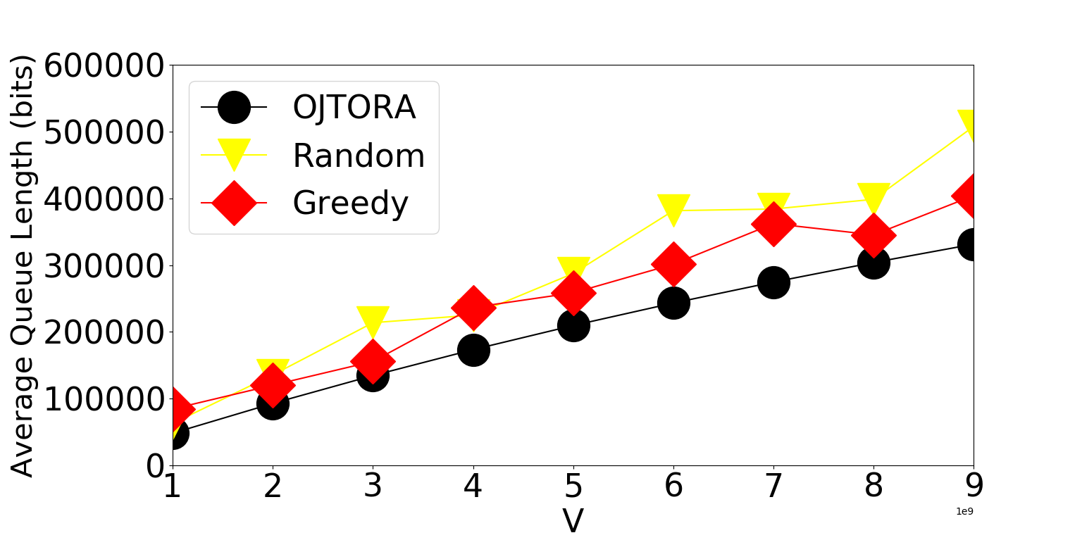
As shown in Fig. 4, as $V$ increases, the average service capacities achieved by all three approaches decrease. However, the average service costs increase. According to (22) and (24), as $V$ increases, the transmit power consumption of service clients’ devices decreases. This results in the decrease in the average service capacity. With the increase in V, the power consumption increases more rapidly than the latency. As a result, the average service cost increases.

VI-C3 Impact of the Number of Service Clients $n$

As shown in Fig.5, As $n$ increases, the average service cost increases. This is because the competition among service clients for the computing resources on the edge servers becomes fiercer with the increase in $n$ .

VI-C4 The Impact of the Number of Edge Servers $m$

As shown in Fig.6, with the increase in $m$ , the average power consumption, the average queue length and the average service cost increase. However, when $m$ continues to increase, the average service cost converges and remains steady. This is because the resources are more than sufficient to allow all service clients to be served.

VII Conclusion

In this paper, we investigated a joint task offloading and resource allocation problem in multi-server edge computing environments with the objectives to maximize service capacity, i.e., the number of mobile devices served, and to minimize the service cost, i.e., the service latency and power consumption experienced by service clients. To solve this problem, we proposed OJTORA, an online algorithm based on Lyapunov optimization, which converts the stochastic optimization problem to a per-time-slot deterministic optimization problem. The experimental results show that our approach significantly outperforms two baseline approaches. However, OJTORA does not consider the fairness in the resource sharing among service clients because it assumes static bandwidth allocation for now. In the future, dynamical allocation of bandwidth will be studied. We will also extend OJTORA to accommodate users service clients’ mobility.

References

[1] Y. Mao, C. You, J. Zhang, K. Huang, and K. B. Letaief, “A Survey on Mobile Edge Computing: The Communication Perspective,” IEEE Communications Surveys & Tutorials, vol. 19, no. 4, pp. 2322–2358, 2017.
[2] Y. Zhou and Z. Zhi, “Near-End Cloud Computing: Opportunities and Challenges in the Post-Cloud Computing,” Chinese Journal of Computers, vol. 41, no. 25, pp. 10–19, 2018.
[3] X. Ge, S. Tu, G. Mao, C.-X. Wang, and T. Han, “5G Ultra-Dense Cellular Networks,” IEEE Wireless Communications, vol. 23, no. 1, pp. 72–79, 2016.
[4] Y. Qi, Y. Zhou, L. Liu, L. Tian, and J. Shi, “MEC Coordinated Future 5G Mobile Wireless Networks,” Journal of Computer Research and Development, vol. 55, no. 3, pp. 478–485, 2018.
[5] P. Lai, Q. He, M. Abdelrazek, F. Chen, J. Hosking, J. Grundy, and Y. Yang, “Optimal Edge User Allocation in Edge Computing with Variable Sized Vector Bin Packing,” in International Conference on Service-Oriented Computing (ICSOC). Springer, 2018, pp. 230–245.
[6] L. Zhang, S. Wang, and R. N. Chang, “QCSS: A QoE-aware Control Plane for Adaptive Streaming Service over Mobile Edge Computing Infrastructures,” in IEEE International Conference on Web Services (ICWS). IEEE, 2018, pp. 139–146.
[7] H. Wu, S. Deng, W. Li, M. Fu, J. Yin, and A. Y. Zomaya, “Service Selection for Composition in Mobile Edge Computing Systems,” in IEEE International Conference on Web Services (ICWS). IEEE, 2018, pp. 355–358.
[8] Y. Mao, J. Zhang, S. Song, and K. B. Letaief, “Stochastic Joint Radio and Computational Resource Management for Multi-User Mobile-Edge Computing Systems,” IEEE Transactions on Wireless Communications, vol. 16, no. 9, pp. 5994–6009, 2017.
[9] S. Sardellitti, G. Scutari, and S. Barbarossa, “Joint Optimization of Radio and Computational Resources for Multicell Mobile-Edge Computing,” IEEE Transactions on Signal and Information Processing over Networks, vol. 1, no. 2, pp. 89–103, 2015.
[10] X. Lyu, H. Tian, C. Sengul, and P. Zhang, “Multi-User Joint Task Offloading and Resource Optimization in Proximate Clouds,” IEEE Transactions on Vehicular Technology, vol. 66, no. 4, pp. 3435–3447, 2017.
[11] B. Yu, L. Pu, Y. Xie, J. Xu, and J. Zhang, “Joint Task Offloading and Base Station Association in Mobile Edge Computing,” Journal of Computer Research and Development, vol. 55, no. 3, pp. 537–544, 2018.
[12] T. X. Tran and D. Pompili, “Joint Task Offloading and Resource Allocation for Multi-Server Mobile-Edge Computing Networks,” arXiv preprint arXiv:1705.00704, 2017.
[13] C.-F. Liu, M. Bennis, and H. V. Poor, “Latency and Reliability-Aware Task Offloading and Resource Allocation for Mobile Edge Computing,” in IEEE Global Communications Conference (Globecom Workshops). IEEE, 2017, pp. 1–7.
[14] M. Masoudi, B. Khamidehi, and C. Cavdar, “Green Cloud Computing for Multi Cell Networks,” in Wireless Communications and Networking Conference (WCNC). IEEE, 2017, pp. 1–6.
[15] L. Yang, J. Cao, Z. Wang, and W. Wu, “Network Aware Multi-User Computation Partitioning in Mobile Edge Clouds,” in International Conference on Parallel Processing (ICPP). IEEE, 2017, pp. 302–311.
[16] T. He, H. Khamfroush, S. Wang, T. La Porta, and S. Stein, “It’s Hard to Share: Joint Service Placement and Request Scheduling in Edge Clouds with Sharable and Non-Sharable Resources,” Technical Report, December 2017.[Online]. Available: https://1drv. ms/b/s, Tech. Rep., 2018.
[17] T. Li, C. S. Magurawalage, K. Wang, K. Xu, K. Yang, and H. Wang, “On Efficient Offloading Control in Cloud Radio Access Network with Mobile Edge Computing,” in International Conference on Distributed Computing Systems (ICDCS). IEEE, 2017, pp. 2258–2263.
[18] L. Wang, L. Jiao, J. Li, and M. Mühlhäuser, “Online Resource Allocation for Arbitrary User Mobility in Distributed Edge Clouds,” in Distributed Computing Systems (ICDCS). IEEE, 2017, pp. 1281–1290.
[19] A. Alfayly, I.-H. Mkwawa, L. Sun, and E. Ifeachor, “Qoe-Driven LTE Downlink Scheduling for Voip Application,” in Consumer Communications and Networking Conference (CCNC). IEEE, 2015, pp. 603–604.
[20] A. P. Miettinen and J. K. Nurminen, “Energy Efficiency of Mobile Clients in Cloud Computing,” HotCloud, vol. 10, pp. 4–4, 2010.
[21] S. Han, X. Wang, L. Xu, H. Sun, and N. Zheng, “Frontal Object Perception for Intelligent Vehicles Based on Radar and Camera Fusion,” in Control Conference (CCC). IEEE, 2016, pp. 4003–4008.
[22] X. Chen, “Decentralized Computation Offloading Game for Mobile Cloud Computing,” IEEE Transactions on Parallel and Distributed Systems, vol. 26, no. 4, pp. 974–983, 2015.
[23] Y. Wen, W. Zhang, and H. Luo, “Energy-Optimal Mobile Application Execution: Taming Resource-Poor Mobile Devices with Cloud Clones,” in IEEE International Conference on Computer Communications (INFOCOM). IEEE, 2012, pp. 2716–2720.
[24] T. M. Cover and J. A. Thomas, Elements of Information Theory. John Wiley & Sons, 2012.
[25] A. Ndikumana, N. H. Tran, T. M. Ho, Z. Han, W. Saad, D. Niyato, and C. S. Hong, “Joint Communication, Computation, Caching, and Control in Big Data Multi-Access Edge Computing,” arXiv preprint arXiv:1803.11512, 2018.
[26] M. J. Neely, “Stochastic Network Optimization with Application to Communication and Queueing Systems,” Synthesis Lectures on Communication Networks, vol. 3, no. 1, pp. 1–211, 2010.