跳到论文正文
W Papers独立论文阅读器 arXiv:1903.04392 论文正文 计算阅读时间 · 0%
引用这篇论文根据当前论文元数据生成,正式投稿前建议核对。


License: arXiv.org perpetual non-exclusive license
arXiv:1903.04392v1 [eess.SY] 11 Mar 2019

A Hybrid Controller for Obstacle Avoidance
in an n\displaystyle n-dimensional Euclidean Space

Soulaimane Berkane    Andrea Bisoffi    Dimos V. Dimarogonas Thanks: This research was supported in part by the Swedish Research Council (VR), the European Research Council (ERC) through ERC StG BUCOPHSYS, the Swedish Foundation for Strategic Research (SSF), the EU H2020 Co4Robots project, and the Knut and Alice Wallenberg Foundation (KAW). The authors are with the Department of Automatic Control, KTH Royal Institute of Technology, Sweden. berkane@kth.se (S. Berkane), bisoffi@kth.se (A. Bisoffi), dimos@kth.se (D. V. Dimarogonas).
September 2018
Abstract

For a vehicle moving in an n\displaystyle n-dimensional Euclidean space, we present a construction of a hybrid feedback that guarantees both global asymptotic stabilization of a reference position and avoidance of an obstacle corresponding to a bounded spherical region. The proposed hybrid control algorithm switches between two modes of operation: stabilization (motion-to-goal) and avoidance (boundary-following). The geometric construction of the flow and jump sets of the hybrid controller, exploiting a hysteresis region, guarantees robust switching (chattering-free) between the stabilization and avoidance modes. Simulation results illustrate the performance of the proposed hybrid control approach for a 3-dimensional scenario.

I Introduction

The obstacle avoidance problem is a long lasting problem that has attracted the attention of the robotics and control communities for decades. In a typical robot navigation scenario, the robot is required to reach a given goal (destination) while avoiding to collide with a set of obstacle regions in the workspace. Since the pioneering work by Khatib [1] and the seminal work by Koditscheck and Rimon [2], artificial potential fields or navigation functions have been widely used in the literature, see. e.g., [1, 2, 3, 4], to deal with the obstacle avoidance problem. The idea is to generate an artificial potential field that renders the goal attractive and the obstacles repulsive. Then, by considering trajectories that navigate along the negative gradient of the potential field, one can ensure that the system will reach the desired target from all initial conditions except from a set of measure zero. This is a well known topological obstruction to global asymptotic stabilization by continuous time-invariant feedback when the free state space is not diffeomorphic to a Euclidean space, see, e.g., [5, Thm. 2.2]. This topological obstruction occurs then also in the navigation transform [6] and (control)-barrier-function approaches [7, 8, 9, 10].

To deal with such a limitation, the authors in [11] have proposed a hybrid state feedback controller to achieve robust global asymptotic regulation, in ℝ2\displaystyle\mathbb{R}^{2}, to a target while avoiding an obstacle. This approach has been exploited in [12] to steer a planar vehicle to the source of an unknown but measurable signal while avoiding an obstacle. In [13], a hybrid control law has been proposed to globally asymptotically stabilize a class of linear systems while avoiding an unsafe single point in ℝn\displaystyle\mathbb{R}^{n}.

In this work, we propose a hybrid control algorithm for the global asymptotic stabilization of a single-integrator system that is guaranteed to avoid a non-point spherical obstacle. Our approach considers trajectories in an n−\displaystyle n-dimensional Euclidean space and we resort to tools from higher-dimensional geometry [14] to provide a construction of the flow and jump sets where the different modes of operation of the hybrid controller are activated.

Our proposed hybrid algorithm employs a hysteresis-based switching between the avoidance controller and the stabilizing controller in order to guarantee forward invariance of the obstacle-free region (related to safety) and global asymptotic stability of the reference position. The parameters of the hybrid controller can be tuned so that the hybrid control law matches the stabilizing controller in arbitrarily large subsets of the obstacle-free region.

Preliminaries are in Section II, the problem is formulated in Section III, and our solution is in Sections IV-V, with a numerical exemplification in Section VI. All the proofs of the intermediate lemmas are in the appendix.

II Preliminaries

Throughout the paper, ℝ\displaystyle\mathbb{R} denotes the set of real numbers, ℝn\displaystyle\mathbb{R}^{n} is the n\displaystyle n-dimensional Euclidean space and 𝕊n\displaystyle\mathbb{S}^{n} is the n\displaystyle n-dimensional unit sphere embedded in ℝn+1\displaystyle\mathbb{R}^{n+1}. The Euclidean norm of x∈ℝn\displaystyle x\in\mathbb{R}^{n} is defined as ‖x‖:=x⊤​x\displaystyle\|x\|:=\sqrt{x^{\top}x} and the geodesic distance between two points x\displaystyle x and y\displaystyle y on the sphere 𝕊n\displaystyle\mathbb{S}^{n} is defined by 𝐝𝕊n​(x,y):=arccos⁡(x⊤​y)\displaystyle\mathbf{d}_{\mathbb{S}^{n}}(x,y):=\arccos(x^{\top}y) for all x,y∈𝕊n\displaystyle x,y\in\mathbb{S}^{n}. The closure, interior and boundary of a set 𝒜⊂ℝn\displaystyle\mathcal{A}\subset\mathbb{R}^{n} are denoted as 𝒜¯,𝒜∘\displaystyle\overline{\mathcal{A}},\mathcal{A}^{\circ} and ∂𝒜\displaystyle\partial\mathcal{A}, respectively. The relative complement of a set ℬ⊂ℝn\displaystyle\mathcal{B}\subset\mathbb{R}^{n} with respect to a set 𝒜\displaystyle\mathcal{A} is denoted by 𝒜∖ℬ\displaystyle\mathcal{A}\setminus\mathcal{B} and contains the elements of 𝒜\displaystyle\mathcal{A} which are not in ℬ\displaystyle\mathcal{B}. Given a nonzero vector z∈ℝn∖{0}\displaystyle z\in\mathbb{R}^{n}\setminus\{0\}, we define the maps:

π∥​(z):=z​z⊤‖z‖2,π⟂​(z):=In−z​z⊤‖z‖2,ρ⟂​(z)=In−2​z​z⊤‖z‖2\pi^{\parallel}(z):=\tfrac{zz^{\top}}{\|z\|^{2}},\,\pi^{\perp}(z):=\!I_{n}\!-\tfrac{zz^{\top}}{\|z\|^{2}},\,\rho^{\perp}(z)=\!I_{n}\!-2\tfrac{zz^{\top}}{\|z\|^{2}} (1)

where In\displaystyle I_{n} is the n×n\displaystyle n\times n identity matrix. The map π∥​(⋅)\displaystyle\pi^{\parallel}(\cdot) is the parallel projection map, π⟂​(⋅)\displaystyle\pi^{\perp}(\cdot) is the orthogonal projection map [14], and ρ⟂​(⋅)\displaystyle\rho^{\perp}(\cdot) is the reflector map (also called Householder transformation). Consequently, for any x∈ℝn\displaystyle x\in\mathbb{R}^{n}, the vector π∥​(z)​x\displaystyle\pi^{\parallel}(z)x corresponds to the projection of x\displaystyle x onto the line generated by z\displaystyle z, π⟂​(z)​x\displaystyle\pi^{\perp}(z)x corresponds to the projection of x\displaystyle x onto the hyperplane orthogonal to z\displaystyle z and ρ⟂​(z)​x\displaystyle\rho^{\perp}(z)x corresponds to the reflection of x\displaystyle x about the hyperplane orthogonal to z\displaystyle z. For each z∈n∖{0}\displaystyle z\in\real^{n}\setminus\{0\}, some useful properties of these maps follow:

π∥​(z)​z\displaystyle\displaystyle\pi^{\parallel}(z)z =z,\displaystyle\displaystyle=z, π⟂​(z)​π⟂​(z)\displaystyle\displaystyle\pi^{\perp}(z)\pi^{\perp}(z) =π⟂​(z),\displaystyle\displaystyle=\pi^{\perp}(z), (2)
π⟂​(z)​z\displaystyle\displaystyle\pi^{\perp}(z)z =0,\displaystyle\displaystyle=0, π∥​(z)​π∥​(z)\displaystyle\displaystyle\pi^{\parallel}(z)\pi^{\parallel}(z) =π∥​(z),\displaystyle\displaystyle=\pi^{\parallel}(z), (3)
ρ⟂​(z)​z\displaystyle\displaystyle\rho^{\perp}(z)z =−z,\displaystyle\displaystyle=-z, ρ⟂​(z)​ρ⟂​(z)\displaystyle\displaystyle\rho^{\perp}(z)\rho^{\perp}(z) =In,\displaystyle\displaystyle=I_{n}, (4)
π⟂​(z)​π∥​(z)\displaystyle\displaystyle\pi^{\perp}(z)\pi^{\parallel}(z) =0,\displaystyle\displaystyle=0, π⟂​(z)+π∥​(z)\displaystyle\displaystyle\pi^{\perp}(z)+\pi^{\parallel}(z) =In,\displaystyle\displaystyle=I_{n}, (5)
π∥​(z)​ρ⟂​(z)\displaystyle\displaystyle\pi^{\parallel}(z)\rho^{\perp}(z) =−π∥​(z),\displaystyle\displaystyle=-\pi^{\parallel}(z), 2​π⟂​(z)−ρ⟂​(z)\displaystyle\displaystyle 2\pi^{\perp}(z)-\rho^{\perp}(z) =In,\displaystyle\displaystyle=I_{n}, (6)
π⟂​(z)​ρ⟂​(z)\displaystyle\displaystyle\pi^{\perp}(z)\rho^{\perp}(z) =π⟂​(z),\displaystyle\displaystyle=\pi^{\perp}(z), 2​π∥​(z)+ρ⟂​(z)\displaystyle\displaystyle 2\pi^{\parallel}(z)+\rho^{\perp}(z) =In.\displaystyle\displaystyle=I_{n}. (7)

We define for z∈n∖{0}\displaystyle z\in\real^{n}\setminus\{0\} and θ∈\displaystyle\theta\in\real the parametric map

πθ​(z):=cos2⁡(θ)​π⟂​(z)−sin2⁡(θ)​π∥​(z).\displaystyle\displaystyle\pi^{\theta}(z):=\cos^{2}(\theta)\pi^{\perp}(z)-\sin^{2}(\theta)\pi^{\parallel}(z). (8)
Fig. 1: The helmet region (dark grey) defined in (14).

In (9)–(14), we define for v∈n∖{0}\displaystyle v\in\real^{n}\setminus\{0\} some geometric subsets of ℝn\displaystyle\mathbb{R}^{n}, which are described after (14):

ℬϵ​(c)\displaystyle\displaystyle\mathcal{B}_{\epsilon}(c) :={x∈ℝn:‖x−c‖≤ϵ},\displaystyle\displaystyle:=\{x\in\mathbb{R}^{n}:\|x-c\|\leq\epsilon\}, (9)
ℒ⁡(c,v)\displaystyle\displaystyle\mathcal{L}(c,v) :={x∈ℝn:x=c+λv,λ∈ℝ},\displaystyle\displaystyle:=\{x\in\mathbb{R}^{n}:x=c+\lambda v,\lambda\in\mathbb{R}\}, (10)
𝒫△​(c,v)\displaystyle\displaystyle\mathcal{P}^{\bigtriangleup}(c,v) :={x∈ℝn:v⊤​(x−c)△0},\displaystyle\displaystyle:=\{x\in\mathbb{R}^{n}:v^{\top}(x-c)\bigtriangleup 0\}, (11)
𝒞△​(c,v,θ)\displaystyle\displaystyle\mathcal{C}^{\bigtriangleup}(c,v,\theta) :={x∈ℝn:(x−c)⊤​πθ​(v)​(x−c)△0}\displaystyle\displaystyle:=\{x\in\mathbb{R}^{n}:\!(x\!-c)^{\top}\!\pi^{\theta}\!(v)(x\!-c)\!\bigtriangleup\!0\} (12)
={x∈ℝn:cos2⁡(θ)​‖v‖2​‖x−c‖2△(v⊤​(x−c))2}\displaystyle\displaystyle\!\!\!\!\!\!\!\!\!\!\!\!\!\!\!\!\!\!\!\!=\{x\in\mathbb{R}^{n}:\cos^{2}(\theta)\|v\|^{2}\|x-c\|^{2}\!\bigtriangleup\!(v^{\top}(x-c))^{2}\}
𝒞▽△​(c,v,θ)\displaystyle\displaystyle\mathcal{C}_{\bigtriangledown}^{\bigtriangleup}(c,v,\theta) :=𝒞△​(c,v,θ)∩𝒫▽​(c,v),\displaystyle\displaystyle:=\mathcal{C}^{\bigtriangleup}(c,v,\theta)\cap\mathcal{P}^{\bigtriangledown}(c,v), (13)
ℋ⁡(c,ϵ,ϵ′,μ)\displaystyle\displaystyle\mathcal{H}(c,\epsilon,\epsilon^{\prime},\mu) :=ℬϵ′​(c)∖ℬϵ​(c)∖ℬ‖μ​c‖​(μ​c)¯,\displaystyle\displaystyle:=\overline{\mathcal{B}_{\epsilon^{\prime}}(c)\setminus\mathcal{B}_{\epsilon}(c)\setminus\mathcal{B}_{\|\mu c\|}(\mu c)}, (14)

where the symbols △\displaystyle\bigtriangleup and ▽\displaystyle\bigtriangledown can be selected as △∈{=,<,>,≤,≥}\displaystyle\bigtriangleup\in\{=,<,>,\leq,\geq\} and ▽∈{<,>,≤,≥}\displaystyle\bigtriangledown\in\{<,>,\leq,\geq\}. The set ℬϵ​(c)\displaystyle\mathcal{B}_{\epsilon}(c) in (9) is the ball centered at c∈ℝn\displaystyle c\in\mathbb{R}^{n} with radius ϵ\displaystyle\epsilon. The set ℒ⁡(c,v)\displaystyle\mathcal{L}(c,v) in (10) is the 1−\displaystyle 1-dimensional line passing by the point c∈ℝn\displaystyle c\in\mathbb{R}^{n} and with direction parallel to v\displaystyle v. The set 𝒫=​(c,v)\displaystyle\mathcal{P}^{=}(c,v) in (11) is the (n−1)−\displaystyle(n-1)-dimensional hyperplane that passes through a point c∈ℝn\displaystyle c\in\mathbb{R}^{n} and has normal vector v\displaystyle v. The hyperplane 𝒫=​(c,v)\displaystyle\mathcal{P}^{=}(c,v) divides the Euclidean space ℝn\displaystyle\mathbb{R}^{n} into two closed sets 𝒫≥​(c,v)\displaystyle\mathcal{P}^{\geq}(c,v) and 𝒫≤​(c,v)\displaystyle\mathcal{P}^{\leq}(c,v). The set 𝒞=​(c,v,θ)\displaystyle\mathcal{C}^{=}(c,v,\theta) in (12) is the right circular cone with vertex at c∈ℝn\displaystyle c\in\mathbb{R}^{n}, axis parallel to v\displaystyle v and aperture 2​θ\displaystyle 2\theta. The set 𝒞△​(c,v,θ)\displaystyle\mathcal{C}^{\bigtriangleup}(c,v,\theta) in (12) with ≤\displaystyle\leq as △\displaystyle\bigtriangleup (or ≥\displaystyle\geq as △\displaystyle\bigtriangleup, respectively) is the region inside (or outside, respectively) the cone 𝒞=​(c,v,θ)\displaystyle\mathcal{C}^{=}(c,v,\theta). The plane 𝒫=​(c,v)\displaystyle\mathcal{P}^{=}(c,v) divides the conic region 𝒞△​(c,v,θ)\displaystyle\mathcal{C}^{\bigtriangleup}(c,v,\theta) into two regions 𝒞≤△​(c,v,θ)\displaystyle\mathcal{C}^{\bigtriangleup}_{\leq}(c,v,\theta) and 𝒞≥△​(c,v,θ)\displaystyle\mathcal{C}^{\bigtriangleup}_{\geq}(c,v,\theta) in (13). The set ℋ⁡(c,ϵ,ϵ′,μ)\displaystyle\mathcal{H}(c,\epsilon,\epsilon^{\prime},\mu) in (14) is called a helmet and is obtained by removing from the spherical shell (annulus) ℬϵ′​(c)∖ℬϵ​(c)\displaystyle\mathcal{B}_{\epsilon^{\prime}}(c)\setminus\mathcal{B}_{\epsilon}(c) the portion contained in the ball ℬ‖μ​c‖​(μ​c)\displaystyle\mathcal{B}_{\|\mu c\|}(\mu c), see Fig. 1. The following geometric fact will be used.

Lemma 1

Let c∈ℝn\displaystyle c\in\mathbb{R}^{n} and v1,v2∈𝕊n−1\displaystyle v_{1},v_{2}\in\mathbb{S}^{n-1} be some arbitrary unit vectors such that 𝐝𝕊n−1​(v1,v2)=θ\displaystyle\mathbf{d}_{\mathbb{S}^{n-1}}(v_{1},v_{2})=\theta for some θ∈(0,π]\displaystyle\theta\in(0,\pi]. Let ψ1,ψ2∈[0,π]\displaystyle\psi_{1},\psi_{2}\in[0,\pi] such that ψ1+ψ2<θ<π−(ψ1+ψ2)\displaystyle\psi_{1}+\psi_{2}<\theta<\pi-(\psi_{1}+\psi_{2}). Then

𝒞≤​(c,v1,ψ1)∩𝒞≤​(c,v2,ψ2)={c}.\displaystyle\displaystyle\mathcal{C}^{\leq}(c,v_{1},\psi_{1})\cap\mathcal{C}^{\leq}(c,v_{2},\psi_{2})=\{c\}.

Finally, we consider in this paper hybrid dynamical systems [15], described through constrained differential and difference inclusions for state X∈n\displaystyle X\in\real^{n}:

{X˙∈𝐅⁡(X),X∈ℱ,X+∈𝐉⁡(X),X∈𝒥.\begin{cases}\dot{X}\in\mathbf{F}(X),&X\in\mathcal{F},\\ X^{+}\in\mathbf{J}(X),&X\in\mathcal{J}.\end{cases} (15)

The data of the hybrid system (15) (i.e., the flow set ℱ⊂ℝn\displaystyle\mathcal{F}\subset\mathbb{R}^{n}, the flow map 𝐅:ℝn⇉ℝn\displaystyle\mathbf{F}:\mathbb{R}^{n}\rightrightarrows\mathbb{R}^{n}, the jump set 𝒥⊂ℝn\displaystyle\mathcal{J}\subset\mathbb{R}^{n}, the jump map 𝐉:ℝn⇉ℝn\displaystyle\mathbf{J}:\mathbb{R}^{n}\rightrightarrows\mathbb{R}^{n}) is denoted as ℋ=(ℱ,𝐅,𝒥,𝐉)\displaystyle\mathscr{H}=(\mathbf{\mathcal{F}},\mathbf{F},\mathcal{J},\mathbf{J}).

III Problem Formulation

We consider a vehicle moving in the n\displaystyle n-dimensional Euclidean space according to the following single integrator dynamics:

x˙=u\displaystyle\displaystyle\dot{x}=u (16)

where x∈ℝn\displaystyle x\in\mathbb{R}^{n} is the state of the vehicle and u∈ℝn\displaystyle u\in\mathbb{R}^{n} is the control input. We assume that in the workspace there exists an obstacle considered as a spherical region ℬϵ​(c)\displaystyle\mathcal{B}_{\epsilon}(c) centered at c∈ℝn\displaystyle c\in\mathbb{R}^{n} and with radius ϵ>0\displaystyle\epsilon>0. The vehicle needs to avoid the obstacle while stabilizing its position to a given reference. Without loss of generality we consider n≥2\displaystyle n\geq 2 and take our reference position at x=0\displaystyle x=0 (the origin)11 1 For n=1\displaystyle n=1 (i.e., the state space is a line), global asymptotic stabilization with obstacle avoidance is physically impossible to solve via any feedback..

Assumption 1

‖c‖>ϵ>0\displaystyle\|c\|>\epsilon>0.

Assumption 1 requires that the reference position x=0\displaystyle x=0 is not inside the obstacle region, otherwise the following control objective would not be feasible. Our objective is indeed to design a control strategy for the input u\displaystyle u such that:

  • i)

    the obstacle-free region ℝn∖ℬϵ​(c)\displaystyle\mathbb{R}^{n}\setminus\mathcal{B}_{\epsilon}(c) is forward invariant;

  • ii)

    the origin x=0\displaystyle x=0 is globally asymptotically stable;

  • iii)

    for each ϵ′>ϵ\displaystyle\epsilon^{\prime}>\epsilon, there exist controller parameters such that the control law matches, in ℝn∖ℬϵ′​(c)\displaystyle\mathbb{R}^{n}\setminus\mathcal{B}_{\epsilon^{\prime}}(c), the law u=−k0​x\displaystyle u=-k_{0}x (k0>0\displaystyle k_{0}>0) used in the absence of the obstacle.

Objective i) guarantees that all trajectories of the closed-loop system are safely avoiding the obstacle by remaining outside the obstacle region. Objectives i) and ii), together, can not be achieved using a continuous feedback due to the topological obstruction discussed in the introduction. Objective iii) is the so-called semiglobal preservation property [13]. This property is desirable when the original controller parameters are optimally tuned and the controller modifications imposed by the presence of the obstacle should be as minimal as possible. Such a property is also accounted for in the quadratic programming formulation of [16, III.A.]. The obstacle avoidance problem described above is solved via a hybrid feedback strategy in Sections IV-V.

IV Proposed Hybrid Control Algorithm for Obstacle Avoidance

In this section, we propose a hybrid controller that switches suitably between an avoidance controller and a stabilizing controller. Let m∈{−1,0,1}\displaystyle m\in\{-1,0,1\} be a discrete variable dictating the control mode where m=0\displaystyle m=0 corresponds to the activation of the stabilizing controller and |m|=1\displaystyle|m|=1 corresponds to the activation of the avoidance controller, which has two configurations m∈{−1,1}\displaystyle m\in\{-1,1\}. The proposed control input, depending on both the state x∈ℝn\displaystyle x\in\mathbb{R}^{n} and the control mode m∈{−1,0,1}\displaystyle m\in\{-1,0,1\}, is given by the feedback law

u\displaystyle u =κ⁡(x,m):={−k0​x,m=0−km​π⟂​(x−c)​(x−pm),m∈{−1, 1}\displaystyle=\kappa(x,m):=\begin{cases}-k_{0}x,&m=0\\ -k_{m}\pi^{\perp}(x-c)(x-p_{m}),&m\in\{-1,\,1\}\end{cases}

where km>0\displaystyle k_{m}>0 (with m∈{−1,0,1}\displaystyle m\in\{-1,0,1\}) and pm∈ℝn\displaystyle p_{m}\in\mathbb{R}^{n} (with m∈{−1,1}\displaystyle m\in\{-1,1\}) are design parameters. During the stabilization mode (m=0\displaystyle m=0), the control input above steers x\displaystyle x towards x=0\displaystyle x=0. During the avoidance mode (|m|=1\displaystyle|m|=1), the control input above minimizes the distance to the auxiliary attractive point pm\displaystyle p_{m} while maintaining a constant distance to the center of the ball ℬϵ​(c)\displaystyle\mathcal{B}_{\epsilon}(c), thereby avoiding to hit the obstacle. This is done by projecting the feedback −km​(x−pm)\displaystyle-k_{m}(x-p_{m}) on the hyperplane orthogonal to (x−c)\displaystyle(x-c). This control strategy resembles the well-known path planning Bug algorithms (see, e.g., [17]) where the motion planner switches between motion-to-goal objective and boundary-following objective. We refer the reader to Fig. 2 from now onward for all of this section. For θ>0\displaystyle\theta>0 (further bounded in (21)), the points p1,p−1\displaystyle p_{1},p_{-1} are selected to lie on the cone22 2 Following the remark in Footnote 1, note that the set 𝒞≤=​(c,c,θ)∖{c}\displaystyle\mathcal{C}^{=}_{\leq}(c,c,\theta)\setminus\{c\} is nonempty for all n≥2\displaystyle n\geq 2. 𝒞≤=​(c,c,θ)∖{c}\displaystyle\mathcal{C}^{=}_{\leq}(c,c,\theta)\setminus\{c\}:

p1∈𝒞≤=​(c,c,θ)∖{c}​ and ​p−1:=−ρ⟂​(c)​p1.\displaystyle\displaystyle p_{1}\in\mathcal{C}^{=}_{\leq}(c,c,\theta)\setminus\{c\}\text{ and }p_{-1}:=-\rho^{\perp}(c)p_{1}. (17)

Note that, by (17), p−1\displaystyle p_{-1} opposes p1\displaystyle p_{1} diametrically with respect to the axis of the cone 𝒞≤=​(c,c,θ)\displaystyle\mathcal{C}^{=}_{\leq}(c,c,\theta) and also belongs to 𝒞≤=​(c,c,θ)∖{c}\displaystyle\mathcal{C}^{=}_{\leq}(c,c,\theta)\setminus\{c\} as shown in the following lemma.

Lemma 2

p−1∈𝒞≤=​(c,c,θ)∖{c}.\displaystyle p_{-1}\in\mathcal{C}^{=}_{\leq}(c,c,\theta)\setminus\{c\}.

The logic variable m\displaystyle m is selected according to a hybrid mechanism that exploits a suitable construction of the flow and jump sets. This hybrid selection is obtained through the hybrid dynamical system

{x˙=κ⁡(x,m)m˙=0\displaystyle\displaystyle\left\{\begin{aligned} \dot{x}&=\kappa(x,m)\\ \dot{m}&=0\end{aligned}\right. (x,m)∈⋃m∈{−1,0,1}ℱm×{m}\displaystyle\displaystyle(x,m)\in\bigcup_{m\in\{-1,0,1\}}\!\!\!\!\mathcal{F}_{m}\times\{m\} (18a)
{x+=xm+∈𝐌⁡(x,m)\displaystyle\displaystyle\left\{\begin{aligned} x^{+}&=x\\ m^{+}&\in\mathbf{M}(x,m)\end{aligned}\right. (x,m)∈⋃m∈{−1,0,1}𝒥m×{m}.\displaystyle\displaystyle(x,m)\in\bigcup_{m\in\{-1,0,1\}}\!\!\!\!\mathcal{J}_{m}\times\{m\}. (18b)
The flow and jump sets for each mode m∈{−1,0,1}\displaystyle m\in\{-1,0,1\} are defined as (see (14) for the definition of the helmet ℋ\displaystyle\mathcal{H}):
ℱ0:=ℝn∖(𝒥0∪ℬϵ​(c))¯,\displaystyle\displaystyle\mathcal{F}_{0}:=\overline{\mathbb{R}^{n}\setminus(\mathcal{J}_{0}\cup\mathcal{B}_{\epsilon}(c))}, (18c)
𝒥0:=ℋ⁡(c,ϵ,ϵs,1/2),\displaystyle\displaystyle\mathcal{J}_{0}:=\mathcal{H}(c,\epsilon,\epsilon_{s},1/2), (18d)
ℱm:=ℋ⁡(c,ϵ,ϵh,μ)∩𝒞≤≥​(c,pm−c,ψ),\displaystyle\displaystyle\mathcal{F}_{m}:=\mathcal{H}(c,\epsilon,\epsilon_{h},\mu)\cap\mathcal{C}_{\leq}^{\geq}(c,p_{m}-c,\psi), |m|=1,\displaystyle\displaystyle|m|=1, (18e)
𝒥m:=ℝn∖(ℱm∪ℬϵ​(c))¯,\displaystyle\displaystyle\mathcal{J}_{m}:=\overline{\mathbb{R}^{n}\setminus(\mathcal{F}_{m}\cup\mathcal{B}_{\epsilon}(c))}, |m|=1,\displaystyle\displaystyle|m|=1, (18f)
see their depiction in Fig. 2, and the (set-valued) jump map is defined as
𝐌⁡(x,0)\displaystyle\displaystyle\mathbf{M}(x,0) :={m′∈{−1,1}:x∈𝒞≥​(c,pm′−c,ψ¯)}\displaystyle\displaystyle\!:=\left\{m^{\prime}\!\in\!\{-1,1\}\colon x\in\mathcal{C}^{\geq}(c,p_{m^{\prime}}\!-c,\bar{\psi})\right\} (18g)
𝐌⁡(x,m)\displaystyle\displaystyle\mathbf{M}(x,m) :=0, for ​m∈{−1,1},\displaystyle\displaystyle\!:=0,\quad\text{ for }m\in\{-1,1\}, (18h)
Fig. 2: 2D illustration of flow and jump sets considered in Sections IV-V.

where ϵs\displaystyle\epsilon_{s}, ϵh\displaystyle\epsilon_{h}, θ\displaystyle\theta, ψ\displaystyle\psi, ψ¯\displaystyle\bar{\psi} are design parameters selected later as in Assumption 2. Before we state our main result, a discussion motivating the above construction of flow and jump sets is in order.

During the stabilization mode m=0\displaystyle m=0, the closed-loop system should not flow when x\displaystyle x is close enough to the surface of the obstacle region ℬϵ​(c)\displaystyle\mathcal{B}_{\epsilon}(c) and the vector field −k0​x\displaystyle-k_{0}x points inside ℬϵ​(c)\displaystyle\mathcal{B}_{\epsilon}(c). Indeed, by computing the time derivative of ‖x−c‖2\displaystyle\|x-c\|^{2}, we can obtain the set where the stabilizing vector field −k0​x\displaystyle-k_{0}x causes a decrease in the distance ‖x−c‖2\displaystyle\|x-c\|^{2} to the centre of the obstacle region ℬϵ​(c)\displaystyle\mathcal{B}_{\epsilon}(c). This set is characterized by the inequality

−k0​x⊤​(x−c)≤0⟺‖x−c/2‖2≥‖c/2‖2.\displaystyle\displaystyle-k_{0}x^{\top}(x-c)\leq 0\Longleftrightarrow\left\|x-{c}/{2}\right\|^{2}\geq\left\|{c}/{2}\right\|^{2}. (19)

The closed set in (19) corresponds to the region outside the ball ℬ‖c/2‖​(c/2)\displaystyle\mathcal{B}_{\|c/2\|}(c/2). Therefore, to keep the vehicle safe during the stabilization mode, we define around the obstacle a helmet region ℋ⁡(c,ϵ,ϵs,1/2)\displaystyle\mathcal{H}(c,\epsilon,\epsilon_{s},1/2), which is used as the jump set 𝒥0\displaystyle\mathcal{J}_{0} in (18d). In other words, if during the stabilization mode the vehicle hits this safety helmet, then the controller jumps to avoidance mode. The amount ϵs−ϵ\displaystyle\epsilon_{s}-\epsilon represents the thickness of the safety helmet that defines the jump set 𝒥0\displaystyle\mathcal{J}_{0}.

During the avoidance mode |m|=1\displaystyle|m|=1, we want our controller to slide on the helmet ℋ⁡(c,ϵ,ϵh,μ)\displaystyle\mathcal{H}(c,\epsilon,\epsilon_{h},\mu) while maintaining a constant distance to the center c\displaystyle c. Note that, with ϵh>ϵs\displaystyle\epsilon_{h}>\epsilon_{s} and μ<1/2\displaystyle\mu<1/2, the helmet ℋ⁡(c,ϵ,ϵh,μ)\displaystyle\mathcal{H}(c,\epsilon,\epsilon_{h},\mu) (see also Fig. 1) is an inflated version of the helmet ℋ⁡(c,ϵ,ϵs,1/2)\displaystyle\mathcal{H}(c,\epsilon,\epsilon_{s},1/2) and creates a hysteresis region useful to prevent infinitely many consecutive jumps (Zeno behavior). Let us then characterize in the following lemma the equilibria of the avoidance vector field κ⁡(x,m)=−km​π⟂​(x−c)​(x−pm)\displaystyle\kappa(x,m)=-k_{m}\pi^{\perp}(x-c)(x-p_{m}) (|m|=1\displaystyle|m|=1).

Lemma 3

For each x∈n∖{c}\displaystyle x\in\real^{n}\setminus\{c\} and m∈{−1,1}\displaystyle m\in\{-1,1\}, π⟂​(x−c)​(x−pm)=0\displaystyle\pi^{\perp}(x-c)(x-p_{m})=0 if and only if x∈ℒ⁡(c,pm−c)\displaystyle x\in\mathcal{L}(c,p_{m}-c).

Since we want the trajectories to leave the set ℱm\displaystyle\mathcal{F}_{m} during the avoidance mode, it is necessary to select the point pm\displaystyle p_{m} and the flow set ℱm\displaystyle\mathcal{F}_{m} such that ℒ⁡(c,pm−c)∩ℱm=∅\displaystyle\mathcal{L}(c,p_{m}-c)\cap\mathcal{F}_{m}=\emptyset for each m∈{−1,1}\displaystyle m\in\{-1,1\}, otherwise trajectories can stay in the avoidance mode indefinitely. This motivates the intersection with the conic region in (18e) and Lemma 4, in view of which we pose the following assumption.

Assumption 2

The parameters in (18) are selected as:

ϵh∈(ϵ,ϵ​‖c‖)\displaystyle\displaystyle\epsilon_{h}\in\big(\epsilon,\sqrt{\epsilon\|c\|}\big) ϵs∈(ϵ,ϵh)\displaystyle\displaystyle\epsilon_{s}\in(\epsilon,\epsilon_{h}) μ∈(μmin,1/2)\displaystyle\displaystyle\mu\in(\mu_{\min},1/2) (20)
θ∈(0,θmax)\displaystyle\displaystyle\theta\in(0,\theta_{\max}) ψ∈(0,ψmax)\displaystyle\displaystyle\psi\in(0,\psi_{\max}) ψ¯∈(ψ,ψmax)\displaystyle\displaystyle\bar{\psi}\in(\psi,\psi_{\max}) (21)

where μmin\displaystyle\mu_{\min}, θmax\displaystyle\theta_{\max} and ψmax\displaystyle\psi_{\max} are defined as

μmin:=12​ϵh2+‖c‖2−2​ϵ​‖c‖‖c‖2−ϵ​‖c‖∈(0,1/2),\displaystyle\displaystyle\mu_{\min}:=\frac{1}{2}\frac{\epsilon_{h}^{2}+\|c\|^{2}-2\epsilon\|c\|}{\|c\|^{2}-\epsilon\|c\|}\in(0,{1}/{2}), (22)
θmax:=arccos⁡(ϵh2+‖c‖2​(1−2​μ)2​ϵ​‖c‖​(1−μ))∈(0,π/2),\displaystyle\displaystyle\theta_{\max}:=\arccos\left(\frac{\epsilon_{h}^{2}+\|c\|^{2}(1-2\mu)}{2\epsilon\|c\|(1-\mu)}\right)\in(0,{\pi}/{2}), (23)
ψmax:=min⁡(θ,π/2−θ)∈(0,π/4).\displaystyle\displaystyle\psi_{\max}:=\min(\theta,\pi/2-\theta)\in(0,\pi/4). (24)

The intervals in (20)–(24) are well defined. They can be checked in this order. The intervals of ϵh\displaystyle\epsilon_{h} and ϵs\displaystyle\epsilon_{s} are well defined by Assumption 1. Then, those of μmin\displaystyle\mu_{\min}, μ\displaystyle\mu, θmax\displaystyle\theta_{\max} (θmax>0\displaystyle\theta_{\max}>0 directly from μ>μmin\displaystyle\mu>\mu_{\min}), θ\displaystyle\theta, ψmax\displaystyle\psi_{\max} and, finally, those of ψ\displaystyle\psi and ψ¯\displaystyle\bar{\psi} (corresponding to 0<ψ<ψ¯<ψmax\displaystyle 0<\psi<\bar{\psi}<\psi_{\max}) are also well defined.

Lemma 4

Under Assumption 2, ℱm∩ℒ⁡(c,pm−c)=∅\displaystyle\mathcal{F}_{m}\cap\mathcal{L}(c,p_{m}-c)=\emptyset, for m∈{−1,1}\displaystyle m\in\{-1,1\}.

V Main Result

In this section, we state and prove our main result, which corresponds to the objectives discussed in Section III. Let us first write more compactly flow/jump sets and maps:

ℱ:=⋃m∈{−1,0,1}\displaystyle\displaystyle\mathcal{F}:=\!\!\!\!\bigcup_{m\in\{-1,0,1\}}\!\!\!\! ℱm×{m},𝒥:=⋃m∈{−1,0,1}𝒥m×{m}\displaystyle\displaystyle\mathcal{F}_{m}\times\{m\},\,\mathcal{J}:=\!\!\!\!\bigcup_{m\in\{-1,0,1\}}\!\!\!\!\mathcal{J}_{m}\times\{m\} (25)
(x,m)\displaystyle\displaystyle(x,m) ↦𝐅⁡(x,m):=(κ⁡(x,m),0),\displaystyle\displaystyle\mapsto\mathbf{F}(x,m):=(\kappa(x,m),0), (26)
(x,m)\displaystyle\displaystyle(x,m) ↦𝐉⁡(x,m):=(x,𝐌⁡(x,m)).\displaystyle\displaystyle\mapsto\mathbf{J}(x,m):=(x,\mathbf{M}(x,m)). (27)

The mild regularity conditions satisfied by the hybrid system (18), as in the next lemma, guarantee the applicability of many results in the proof of our main result.

Lemma 5

The hybrid system with data (ℱ,𝐅,𝒥,𝐉)\displaystyle(\mathcal{F},\mathbf{F},\mathcal{J},\mathbf{J}) satisfies the hybrid basic conditions in [15, Ass. 6.5].

Let us define the obstacle-free set 𝒦\displaystyle\mathcal{K} and the attractor 𝒜\displaystyle\mathcal{A} as:

𝒦:=ℝn∖ℬϵ​(c)¯×{−1,0,1},𝒜:={0}×{0}.\mathcal{K}:=\overline{\mathbb{R}^{n}\setminus\mathcal{B}_{\epsilon}(c)}\times\{-1,0,1\},\quad\mathcal{A}:=\{0\}\times\{0\}. (28)

Our main result is given in the following theorem.

Theorem 1

Consider the hybrid system (18) under Assumptions 1-2. Then,

  • i)

    all maximal solutions do not have finite escape times, are complete in the ordinary time direction, and the obstacle-free set 𝒦\displaystyle\mathcal{K} in (28) is forward invariant;

  • ii)

    the set 𝒜\displaystyle\mathcal{A} in (28) is globally asymptotically stable;

  • iii)

    for each ϵ′>ϵ\displaystyle\epsilon^{\prime}>\epsilon, it is possible to tune the hybrid controller parameters so that the resulting hybrid feedback law matches, in ℝn∖ℬϵ′​(c)\displaystyle\mathbb{R}^{n}\setminus\mathcal{B}_{\epsilon^{\prime}}(c), the law u=−k0​x\displaystyle u=-k_{0}x.

Theorem 1 shows that the three objectives discussed in Section III are fulfilled.

V-A Proof of Theorem 1

Set to which x belongs𝐓ℱ0​(x)∂ℬϵ​(c)∩ℬ‖c/2‖∘​(c/2)𝒫≥​(0,x−c)∂ℬϵs​(c)∖ℬ‖c/2‖​(c/2)𝒫≥​(0,x−c)(∂ℬ‖c/2‖​(c/2)∩ℬϵs∘​(c))∖ℬϵ​(c)𝒫≤​(0,x−c/2)∂ℬϵ​(c)∩∂ℬ‖c/2‖​(c/2)𝒫≥​(0,x−c)∩𝒫≤​(0,x−c/2)∂ℬ‖c/2‖​(c/2)∩∂ℬϵs​(c)𝒫≥​(0,x−c)∪𝒫≤​(0,x−c/2)\begin{array}[]{ll}\hline\cr\hline\cr\text{Set to which $\displaystyle x$ belongs}&\mathbf{T}_{\mathcal{F}_{0}}(x)\\ \hline\cr\partial\mathcal{B}_{\epsilon}(c)\cap\mathcal{B}^{\circ}_{\|c/2\|}(c/2)&\mathcal{P}^{\geq}(0,x-c)\\ \partial\mathcal{B}_{\epsilon_{s}}(c)\setminus\mathcal{B}_{\|c/2\|}(c/2)&\mathcal{P}^{\geq}(0,x-c)\\ (\partial\mathcal{B}_{\|c/2\|}(c/2)\cap\mathcal{B}^{\circ}_{\epsilon_{s}}(c))\setminus\mathcal{B}_{\epsilon}(c)&\mathcal{P}^{\leq}(0,x-c/2)\\ \partial\mathcal{B}_{\epsilon}(c)\cap\partial\mathcal{B}_{\|c/2\|}(c/2)&\mathcal{P}^{\geq}(0,x-c)\cap\mathcal{P}^{\leq}(0,x-c/2)\\ \partial\mathcal{B}_{\|c/2\|}(c/2)\cap\partial\mathcal{B}_{\epsilon_{s}}(c)&\mathcal{P}^{\geq}(0,x-c)\cup\mathcal{P}^{\leq}(0,x-c/2)\\ \hline\cr\hline\cr\end{array}
Set to which x belongs𝐓ℱm¯​(x)∂ℬϵ​(c)∖ℬ‖μ​c‖​(μ​c)∖𝒞≤​(c,pm¯−c,ψ)𝒫≥​(0,x−c)∂ℬϵh​(c)∖ℬ‖μ​c‖​(μ​c)∖𝒞≤​(c,pm¯−c,ψ)𝒫≤​(0,x−c)∂ℬ‖μ​c‖​(μ​c)∩ℬϵh∘​(c)∖ℬϵ​(c)𝒫≥​(0,x−μ​c)𝒞≤=​(c,pm¯−c,ψ)∩ℬϵh∘​(c)∖ℬϵ​(c)𝒫≥​(0,nm¯​(x))∂ℬϵ​(c)∩∂ℬ‖μ​c‖​(μ​c)𝒫≥​(0,x−c)∩𝒫≥​(0,x−μ​c)∂ℬϵh​(c)∩∂ℬ‖μ​c‖​(μ​c)𝒫≤​(0,x−c)∩𝒫≥​(0,x−μ​c)∂ℬϵ​(c)∩𝒞=​(c,pm¯−c,ψ)𝒫≥​(0,x−c)∩𝒫≥​(0,nm¯​(x))∂ℬϵh​(c)∩𝒞=​(c,pm¯−c,ψ)𝒫≤​(0,x−c)∩𝒫≥​(0,nm¯​(x))\begin{array}[]{ll}\hline\cr\hline\cr\text{Set to which $\displaystyle x$ belongs}&\mathbf{T}_{\mathcal{F}_{\bar{m}}}(x)\\ \hline\cr\partial\mathcal{B}_{\epsilon}(c)\!\setminus\!\mathcal{B}_{\|\mu c\|}(\mu c)\!\setminus\!\mathcal{C}^{\leq}(c,p_{\bar{m}}\!-\!c,\psi)&\mathcal{P}^{\geq}(0,x-c)\\ \partial\mathcal{B}_{\epsilon_{h}}\!(c)\!\setminus\!\mathcal{B}_{\|\mu c\|}\!(\mu c)\!\setminus\!\mathcal{C}^{\leq}(c,p_{\bar{m}}\!-\!c,\psi)&\mathcal{P}^{\leq}(0,x-c)\\ \partial\mathcal{B}_{\|\mu c\|}(\mu c)\cap\mathcal{B}^{\circ}_{\epsilon_{h}}(c)\setminus\mathcal{B}_{\epsilon}(c)&\mathcal{P}^{\geq}(0,x-\mu c)\\ \mathcal{C}^{=}_{\leq}(c,p_{\bar{m}}-c,\psi)\cap\mathcal{B}^{\circ}_{\epsilon_{h}}(c)\setminus\mathcal{B}_{\epsilon}(c)&\mathcal{P}^{\geq}(0,n_{\bar{m}}(x))\\ \partial\mathcal{B}_{\epsilon}(c)\cap\partial\mathcal{B}_{\|\mu c\|}(\mu c)&\mathcal{P}^{\geq}(0,x\!-\!c)\!\cap\!\mathcal{P}^{\geq}(0,x-\mu c)\\ \partial\mathcal{B}_{\epsilon_{h}}(c)\cap\partial\mathcal{B}_{\|\mu c\|}(\mu c)&\mathcal{P}^{\leq}(0,x\!-\!c)\!\cap\!\mathcal{P}^{\geq}(0,x-\mu c)\\ \partial\mathcal{B}_{\epsilon}(c)\cap\mathcal{C}^{=}(c,p_{\bar{m}}-c,\psi)&\mathcal{P}^{\geq}(0,x\!-\!c)\!\cap\!\mathcal{P}^{\geq}(0,n_{\bar{m}}(x))\\ \partial\mathcal{B}_{\epsilon_{h}}(c)\cap\mathcal{C}^{=}(c,p_{\bar{m}}-c,\psi)&\mathcal{P}^{\leq}(0,x\!-\!c)\!\cap\!\mathcal{P}^{\geq}(0,n_{\bar{m}}(x))\\ \hline\cr\hline\cr\end{array}
TABLE I: Points (x,m)\displaystyle(x,m) and their tangent cones (m¯\displaystyle\bar{m} is either −1\displaystyle-1 or 1\displaystyle 1 and nm¯​(x):=πψ​(pm¯−c)​(x−c)\displaystyle n_{\bar{m}}(x):=\pi^{\psi}(p_{\bar{m}}-c)(x-c)).

To prove item i), we resort to [18, Thm. 4.3]. We first establish for ℋ\displaystyle\mathscr{H} in (18) the relationships invoked in [18, Thm. 4.3], and we refer the reader to Fig. 2 for a two-dimensional visualization. In particular, the boundary of the flow set ℱ\displaystyle\mathcal{F} is given by ∂ℱ={(x,m):x∈∂ℱm}\displaystyle\partial\mathcal{F}=\{(x,m):x\in\partial\mathcal{F}_{m}\}, where the sets ∂ℱ0\displaystyle\partial\mathcal{F}_{0} and ∂ℱm,m∈{−1,1}\displaystyle\partial\mathcal{F}_{m},m\in\{-1,1\}, are

∂ℱ0\displaystyle\displaystyle\partial\mathcal{F}_{0} =(∂ℬϵ​(c)∩ℬ‖c/2‖​(c/2))∪(∂ℬϵs​(c)∖ℬ‖c/2‖​(c/2))\displaystyle\displaystyle=\big(\partial\mathcal{B}_{\epsilon}(c)\cap\mathcal{B}_{\|c/2\|}(c/2)\big)\cup\big(\partial\mathcal{B}_{\epsilon_{s}}(c)\setminus\mathcal{B}_{\|c/2\|}(c/2)\big)
∪((∂ℬ‖c/2‖​(c/2)∩ℬϵs​(c))∖ℬϵ​(c)),\displaystyle\displaystyle\quad\cup\big((\partial\mathcal{B}_{\|c/2\|}(c/2)\cap\mathcal{B}_{\epsilon_{s}}(c))\setminus\mathcal{B}_{\epsilon}(c)\big),
∂ℱm\displaystyle\displaystyle\partial\mathcal{F}_{m} =((∂ℬϵ​(c)∪∂ℬϵh​(c))∖ℬ‖μ​c‖​(μ​c)∖𝒞≤≤​(c,pm−c,ψ))\displaystyle\displaystyle=\big((\partial\mathcal{B}_{\epsilon}(c)\cup\partial\mathcal{B}_{\epsilon_{h}}(c))\setminus\mathcal{B}_{\|\mu c\|}(\mu c)\setminus\mathcal{C}^{\leq}_{\leq}(c,p_{m}-c,\psi)\big)
∪((∂ℬ‖μ​c‖​(μ​c)∪𝒞≤=​(c,pm−c,ψ))∩ℬϵh​(c)∖ℬϵ∘​(c)).\displaystyle\displaystyle\cup\big((\partial\mathcal{B}_{\|\mu c\|}(\mu c)\cup\mathcal{C}^{=}_{\leq}(c,p_{m}-c,\psi))\cap\mathcal{B}_{\epsilon_{h}}(c)\setminus\mathcal{B}^{\circ}_{\epsilon}(c)\big).

The tangent cone33 3 For the definition of tangent cone, see [15, Def. 5.12 and Fig. 5.4]., evaluated at the boundary of ℱ\displaystyle\mathcal{F}, is given in Table I. Consider m=0\displaystyle m=0 and let z:=κ⁡(x,0)=−k0​x\displaystyle z:=\kappa(x,0)=-k_{0}x. If x∈∂ℬϵ​(c)∩ℬ‖c/2‖∘​(c/2)\displaystyle x\in\partial\mathcal{B}_{\epsilon}(c)\cap\mathcal{B}^{\circ}_{\|c/2\|}(c/2) then one has (x−c)⊤​z=−k0​x⊤​(x−c)>0\displaystyle(x-c)^{\top}z=-k_{0}x^{\top}(x-c)>0 (since x∈ℬ‖c/2‖∘​(c/2)\displaystyle x\in\mathcal{B}^{\circ}_{\|c/2\|}(c/2), see (19)), i.e., z∈𝒫>​(0,x−c)\displaystyle z\in\mathcal{P}^{>}(0,x-c). If x∈(∂ℬ‖c/2‖​(c/2)∩ℬϵs∘​(c))∖ℬϵ​(c)\displaystyle x\in(\partial\mathcal{B}_{\|c/2\|}(c/2)\cap\mathcal{B}^{\circ}_{\epsilon_{s}}(c))\setminus\mathcal{B}_{\epsilon}(c) then one has (x−c/2)⊤z=−k0x⊤(x−c/2)=−k0x⊤c/2=−k0∥x∥2/2≤0\displaystyle(x-c/2)^{\top}z=-k_{0}x^{\top}(x-c/2)=-k_{0}x^{\top}c/2=-k_{0}\|x\|^{2}/2\leq 0 since x⊤​(x−c)=0\displaystyle x^{\top}(x-c)=0 from ‖x−c/2‖=‖c/2‖\displaystyle\|x-c/2\|=\|c/2\|. Then, z∈𝒫≤​(0,x−c/2)\displaystyle z\in\mathcal{P}^{\leq}(0,x-c/2). If x∈∂ℬϵ​(c)∩∂ℬ‖c/2‖​(c/2)\displaystyle x\in\partial\mathcal{B}_{\epsilon}(c)\cap\partial\mathcal{B}_{\|c/2\|}(c/2) or x∈∂ℬ‖c/2‖​(c/2)∩∂ℬϵs​(c)\displaystyle x\in\partial\mathcal{B}_{\|c/2\|}(c/2)\cap\partial\mathcal{B}_{\epsilon_{s}}(c) then z⊤​(x−c)=0\displaystyle z^{\top}(x-c)=0 and z⊤(x−c/2)=−k0∥x∥2/2≤0\displaystyle z^{\top}(x-c/2)=-k_{0}\|x\|^{2}/2\leq 0 showing, respectively, that z∈𝒫≥​(0,x−c)∩𝒫≤​(0,x−c/2)\displaystyle z\in\mathcal{P}^{\geq}(0,x-c)\cap\mathcal{P}^{\leq}(0,x-c/2). Finally, if x∈∂ℬϵs​(c)∖ℬ‖c/2‖​(c/2)\displaystyle x\in\partial\mathcal{B}_{\epsilon_{s}}(c)\setminus\mathcal{B}_{\|c/2\|}(c/2), then one has (x−c)⊤​z=−k0​x⊤​(x−c)<0\displaystyle(x-c)^{\top}z=-k_{0}x^{\top}(x-c)<0 (since x∉ℬ‖c/2‖​(c/2)\displaystyle x\notin\mathcal{B}_{\|c/2\|}(c/2)), i.e., z∈𝒫<​(0,x−c)\displaystyle z\in\mathcal{P}^{<}(0,x-c). Let ℒ0:=∂ℬϵs​(c)∖ℬ‖c/2‖​(c/2)\displaystyle\mathcal{L}_{0}:=\partial\mathcal{B}_{\epsilon_{s}}(c)\setminus\mathcal{B}_{\|c/2\|}(c/2). Therefore, by all the previous arguments,

x∈ℒ0\displaystyle x\in\mathcal{L}_{0} ⟹κ⁡(x,0)∩𝐓ℱ0​(x)=∅\displaystyle\implies\kappa(x,0)\cap\mathbf{T}_{\mathcal{F}_{0}}(x)=\emptyset (29)
x∈∂ℱ0∖ℒ0\displaystyle x\in\partial\mathcal{F}_{0}\setminus\mathcal{L}_{0} ⟹κ⁡(x,0)⊂𝐓ℱ0​(x).\displaystyle\implies\kappa(x,0)\subset\mathbf{T}_{\mathcal{F}_{0}}(x).

Consider then m∈{−1,1}\displaystyle m\in\{-1,1\} and let now z:=κ⁡(x,m)=−km​π⟂​(x−c)​(x−pm)\displaystyle z:=\kappa(x,m)=-k_{m}\pi^{\perp}(x-c)(x-p_{m}). If x∈∂ℬϵ​(c)\displaystyle x\in\partial\mathcal{B}_{\epsilon}(c) or x∈∂ℬϵh​(c)\displaystyle x\in\partial\mathcal{B}_{\epsilon_{h}}(c) then one has (x−c)⊤​z=−km​(x−c)⊤​π⟂​(x−c)​(x−pm)=0\displaystyle(x-c)^{\top}z=-k_{m}(x-c)^{\top}\pi^{\perp}(x-c)(x-p_{m})=0, which implies that both z∈𝒫≥​(0,x−c)\displaystyle z\in\mathcal{P}^{\geq}(0,x-c) and z∈𝒫≤​(0,x−c)\displaystyle z\in\mathcal{P}^{\leq}(0,x-c). Define nm​(x):=πψ​(pm−c)​(x−c)\displaystyle n_{m}(x):=\pi^{\psi}(p_{m}-c)(x-c), which is a normal vector to the cone 𝒞=​(c,pm−c,ψ)\displaystyle\mathcal{C}^{=}(c,p_{m}-c,\psi) at x\displaystyle x. If x∈𝒞≤=​(c,pm−c,ψ)\displaystyle x\in\mathcal{C}^{=}_{\leq}(c,p_{m}-c,\psi), then44 4 Each (in)equality is obtained thanks to the relationship reported over it.

nm​(x)⊤​z=−km​nm​(x)⊤​π⟂​(x−c)​(x−pm)\displaystyle\displaystyle n_{m}(x)^{\top}z=-k_{m}n_{m}(x)^{\top}\pi^{\perp}(x-c)(x-p_{m})
=(3)​km​(x−c)⊤​πψ​(pm−c)​π⟂​(x−c)​(pm−c)\displaystyle\displaystyle\overset{\eqref{eq:propLine2}}{=}k_{m}(x-c)^{\top}\pi^{\psi}(p_{m}-c)\pi^{\perp}(x-c)(p_{m}-c)
=(8),(5)​km​(x−c)⊤​(π⟂​(pm−c)−sin2⁡(ψ)​In)​π⟂​(x−c)​(pm−c)\displaystyle\displaystyle\overset{\eqref{eq:def:piTheta},\eqref{eq:propLine4}}{=}\!k_{m}(x-c)^{\top}\!(\pi^{\perp}\!(p_{m}-c)\!-\!\sin^{2}(\psi)I_{n})\pi^{\perp}\!(x-c)(p_{m}-c)
=(3)​km​(x−c)⊤​π⟂​(pm−c)​π⟂​(x−c)​(pm−c)\displaystyle\displaystyle\overset{\eqref{eq:propLine2}}{=}k_{m}(x-c)^{\top}\pi^{\perp}(p_{m}-c)\pi^{\perp}(x-c)(p_{m}-c)
=(5)​km​(x−c)⊤​π⟂​(pm−c)​(In−π∥​(x−c))​(pm−c)\displaystyle\displaystyle\overset{\eqref{eq:propLine4}}{=}k_{m}(x-c)^{\top}\pi^{\perp}(p_{m}-c)\big(I_{n}-\pi^{\parallel}(x-c)\big)(p_{m}-c)
=(3)−km​(x−c)⊤​π⟂​(pm−c)​π∥​(x−c)​(pm−c)\displaystyle\displaystyle\overset{\eqref{eq:propLine2}}{=}-k_{m}(x-c)^{\top}\pi^{\perp}(p_{m}-c)\pi^{\parallel}(x-c)(p_{m}-c)
=(1)−km​(x−c)⊤​π⟂​(pm−c)​(x−c)‖x−c‖2​(x−c)⊤​(pm−c)≥0\displaystyle\displaystyle\overset{\eqref{eq:proj-refl-maps}}{=}-k_{m}\frac{(x-c)^{\top}\pi^{\perp}(p_{m}-c)(x-c)}{\|x-c\|^{2}}(x-c)^{\top}(p_{m}-c)\geq 0

where the last bound follows from π⟂​(pm−c)\displaystyle\pi^{\perp}(p_{m}-c) positive semidefinite and (x−c)⊤​(pm−c)≤0\displaystyle(x-c)^{\top}(p_{m}-c)\leq 0 (since x∈𝒞≤=​(c,pm−c,ψ)⊂𝒫≤​(c,pm−c)\displaystyle x\in\mathcal{C}^{=}_{\leq}(c,p_{m}-c,\psi)\subset\mathcal{P}^{\leq}(c,p_{m}-c)). Hence, z∈𝒫≥​(0,nm​(x))\displaystyle z\in\mathcal{P}^{\geq}(0,n_{m}(x)). Finally, let x∈∂ℬ‖μ​c‖​(μ​c)∩ℬϵh​(c)∖ℬϵ∘​(c)\displaystyle x\in\partial\mathcal{B}_{\|\mu c\|}(\mu c)\cap\mathcal{B}_{\epsilon_{h}}(c)\setminus\mathcal{B}^{\circ}_{\epsilon}(c). With θmax\displaystyle\theta_{\max} in (23), we have

0≤c⊤​(c−x)≤cos⁡(θmax)​‖c‖​‖x−c‖\displaystyle\displaystyle 0\leq c^{\top}(c-x)\leq\cos(\theta_{\max})\|c\|\|x-c\| (30a)
|(x−c)⊤​(pm−c)|≤‖x−c‖​‖pm−c‖\displaystyle\displaystyle|(x-c)^{\top}(p_{m}-c)|\leq\|x-c\|\|p_{m}-c\| (30b)
c⊤​(pm−c)=−cos⁡(θ)​‖c‖​‖pm−c‖\displaystyle\displaystyle c^{\top}(p_{m}-c)=-\cos(\theta)\|c\|\|p_{m}-c\| (30c)

where the bounds in (30a) follow from (33) in the proof of the previous Lemma 4, μ<1/2\displaystyle\mu<1/2, and x∈∂ℬ‖μ​c‖​(μ​c)∩ℬϵh​(c)∖ℬϵ∘​(c)⊂ℋ⁡(c,ϵ,ϵh,μ)\displaystyle x\in\partial\mathcal{B}_{\|\mu c\|}(\mu c)\cap\mathcal{B}_{\epsilon_{h}}(c)\setminus\mathcal{B}^{\circ}_{\epsilon}(c)\subset\mathcal{H}(c,\epsilon,\epsilon_{h},\mu); (30c) follows from pm∈𝒞≤=​(c,c,θ)\displaystyle p_{m}\in\mathcal{C}^{=}_{\leq}(c,c,\theta) (by (17) and Lemma 2). So

(x−μ​c)⊤​z=−km​(x−μ​c)⊤​π⟂​(x−c)​(x−pm)\displaystyle(x-\mu c)^{\top}z=-k_{m}(x-\mu c)^{\top}\pi^{\perp}(x-c)(x-p_{m})
=(3)​km​(c−μ​c)⊤​π⟂​(x−c)​(pm−c)\displaystyle\overset{\eqref{eq:propLine2}}{=}k_{m}(c-\mu c)^{\top}\pi^{\perp}(x-c)(p_{m}-c)
=(1)​km​(1−μ)​(c⊤​(pm−c)+CLOSE\displaystyle\overset{\eqref{eq:proj-refl-maps}}{=}k_{m}(1-\mu)(c^{\top}(p_{m}-c)+
OPENc⊤​(c−x)​(x−c)⊤​(pm−c)/‖x−c‖2)\displaystyle c^{\top}(c-x)(x-c)^{\top}(p_{m}-c)/\|x-c\|^{2})
≤(30)​km​(1−μ)​(−cos⁡(θ)+cos⁡(θmax))​‖c‖​‖pm−c‖<0\displaystyle\overset{\eqref{eq:proofRel}}{\leq}k_{m}(1-\mu)(-\cos(\theta)+\cos(\theta_{\max}))\|c\|\|p_{m}-c\|<0

since km>0\displaystyle k_{m}>0, 1−μ>0\displaystyle 1-\mu>0 (from (20)) and θ<θmax\displaystyle\theta<\theta_{\max} (from (21)). (x−μ​c)⊤​z<0\displaystyle(x-\mu c)^{\top}z<0 implies then z∈𝒫<​(0,x−μ​c)\displaystyle z\in\mathcal{P}^{<}(0,x-\mu c). Let ℒm:=∂ℬ‖μ​c‖​(μ​c)∩ℬϵh​(c)∖ℬϵ∘​(c)\displaystyle\mathcal{L}_{m}:=\partial\mathcal{B}_{\|\mu c\|}(\mu c)\cap\mathcal{B}_{\epsilon_{h}}(c)\setminus\mathcal{B}^{\circ}_{\epsilon}(c). Therefore, by all the previous arguments,

x∈ℒm\displaystyle x\in\mathcal{L}_{m} ⟹κ⁡(x,m)∩𝐓ℱm​(x)=∅\displaystyle\implies\kappa(x,m)\cap\mathbf{T}_{\mathcal{F}_{m}}(x)=\emptyset (31)
x∈∂ℱm∖ℒm\displaystyle x\in\partial\mathcal{F}_{m}\setminus\mathcal{L}_{m} ⟹κ⁡(x,m)⊂𝐓ℱm​(x).\displaystyle\implies\kappa(x,m)\subset\mathbf{T}_{\mathcal{F}_{m}}(x).

We can now apply [18, Thm. 4.3]. With 𝒦\displaystyle\mathcal{K} in (28), let ℱ^:=∂(𝒦∩ℱ)∖ℒ\displaystyle\hat{\mathcal{F}}:=\partial(\mathcal{K}\cap\mathcal{F})\setminus\mathcal{L} with ℒ:={(x,m)∈∂ℱ:𝐅⁡(x,m)∩𝐓ℱ​(x,m)=∅}\displaystyle\mathcal{L}:=\{(x,m)\in\partial\mathcal{F}:\mathbf{F}(x,m)\cap\mathbf{T}_{\mathcal{F}}(x,m)=\emptyset\}. By (29) and (31) and 𝒦∩ℱ=ℱ\displaystyle\mathcal{K}\cap\mathcal{F}=\mathcal{F}, we have ℱ^=∪m=−1,0,1(∂ℱm∖ℒm)×{m}\displaystyle\hat{\mathcal{F}}=\cup_{m=-1,0,1}(\partial\mathcal{F}_{m}\setminus\mathcal{L}_{m})\times\{m\} and ℒ=∪m=−1,0,1ℒm×{m}\displaystyle\mathcal{L}=\cup_{m=-1,0,1}\mathcal{L}_{m}\times\{m\}. It follows from (29) and (31) that for every (x,m)∈ℱ^\displaystyle(x,m)\in\hat{\mathcal{F}}, 𝐅⁡(x,m)⊂𝐓ℱ​(x,m)\displaystyle\mathbf{F}(x,m)\subset\mathbf{T}_{\mathcal{F}}(x,m). Also, 𝐉⁡(𝒦∩𝒥)⊂𝒦\displaystyle\mathbf{J}(\mathcal{K}\cap\mathcal{J})\subset\mathcal{K}, ℱ\displaystyle\mathcal{F} is closed, the map 𝐅\displaystyle\mathbf{F} satisfies the hybrid basic conditions as proven in Lemma 5 and it is, moreover, locally Lipschitz since it is continuously differentiable. We conclude then that the set 𝒦\displaystyle\mathcal{K} is forward pre-invariant [18, Def. 3.3]. In addition, since ℒ0⊂𝒥0\displaystyle\mathcal{L}_{0}\subset\mathcal{J}_{0} and ℒm⊂𝒥m\displaystyle\mathcal{L}_{m}\subset\mathcal{J}_{m} with m∈{−1,1}\displaystyle m\in\{-1,1\}, one has ℒ⊂𝒥\displaystyle\mathcal{L}\subset\mathcal{J}. Besides, finite escape times can only occur through flow, and since the sets ℱ−1\displaystyle\mathcal{F}_{-1} and ℱ1\displaystyle\mathcal{F}_{1} are bounded by their definitions in (18e), finite escape times cannot occur for x∈ℱ−1∪ℱ1\displaystyle x\in\mathcal{F}_{-1}\cup\mathcal{F}_{1}. They can neither occur for x∈ℱ0\displaystyle x\in\mathcal{F}_{0} because they would make x⊤​x\displaystyle x^{\top}x grow unbounded, and this would contradict that dd​t​(x⊤​x)≤0\displaystyle\tfrac{d}{dt}(x^{\top}x)\leq 0 by the definition of κ⁡(x,0)\displaystyle\kappa(x,0) and by (18a). Therefore, all maximal solutions do not have finite escape times. By [18, Thm. 4.3] again, the set 𝒦\displaystyle\mathcal{K} is actually forward invariant [18, Def. 3.3], and solutions are complete. Finally, we anticipate here a straightforward corollary of completeness and Lemma 7 below: since the number of jumps is finite by Lemma 7, all maximal solutions to (18) are actually complete in the ordinary time direction.

Now, we will prove item ii) in two steps. First, we prove in the following Lemma 6 that the set 𝒜\displaystyle\mathcal{A} is globally asymptotically stable for the system without jumps. To this end, the jumpless system has data ℋ0=(𝐅,ℱ,∅,∅)\displaystyle\mathscr{H}^{0}=(\mathbf{F},\mathcal{F},\emptyset,\emptyset) with flow map 𝐅\displaystyle\mathbf{F} and flow set ℱ\displaystyle\mathcal{F} defined in (18). We emphasize that ℋ0\displaystyle\mathscr{H}^{0} is obtained in accordance to [19, Eqq. (38)-(39)] by identifying all jumps with events.

Lemma 6

𝒜\displaystyle\mathcal{A} in (28) is globally asymptotically stable for the jumpless hybrid system ℋ0\displaystyle\mathscr{H}^{0}.

Second, we prove in the following Lemma 7 that the number of jumps is finite for the given hybrid dynamics in (18).

Lemma 7

For ℋ\displaystyle\mathscr{H} in (18), each solution starting in 𝒦\displaystyle\mathcal{K} experiences no more than 3\displaystyle 3 jumps.

Based on Lemmas 6-7, global asymptotic stability of 𝒜\displaystyle\mathcal{A} follows straightforwardly from [19, Thm. 31] since the hybrid system in (18) satisfies the Basic Assumptions [19, p. 43], as proven in Lemma 5, the set 𝒜\displaystyle\mathcal{A} is compact and has empty intersection with the jump set.

Lastly, to prove item iii), let ϵ′>ϵ\displaystyle\epsilon^{\prime}>\epsilon. Select the parameter ϵh∈(ϵ,min⁡(ϵ′,ϵ​‖c‖))\displaystyle\epsilon_{h}\in(\epsilon,\min(\epsilon^{\prime},\sqrt{\epsilon\|c\|})) while all other hybrid controller parameters are selected as in Assumption 2. Then this implies that the flow sets ℱm,m∈{−1,1},\displaystyle\mathcal{F}_{m},m\in\{-1,1\}, of the avoidance mode are entirely contained in ℬϵ′​(c)\displaystyle\mathcal{B}_{\epsilon^{\prime}}(c). Therefore, as long as the state x\displaystyle x remains in ℝn∖ℬϵ′​(c)\displaystyle\mathbb{R}^{n}\setminus\mathcal{B}_{\epsilon^{\prime}}(c), solutions are enforced to flow only with the stabilizing mode m=0\displaystyle m=0, which corresponds to the feedback law u=−k0​x\displaystyle u=-k_{0}x.

VI Numerical example

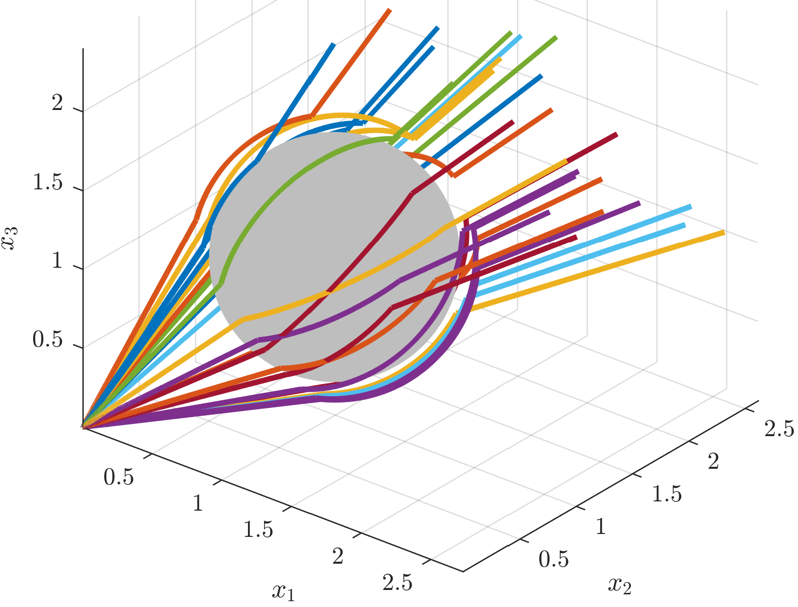
We illustrate our results through a three-dimensional example. The hybrid system in (18) is fully specified by the following parameters. The obstacle has center c=(1,1,1)\displaystyle c=(1,1,1) and radius ϵ=0.700\displaystyle\epsilon=0.700. The controller gains are km=1\displaystyle k_{m}=1 for m∈{−1,0,1}\displaystyle m\in\{-1,0,1\}. The parameters used in the construction of the flow and jump sets are ϵh=0.901\displaystyle\epsilon_{h}=0.901, ϵs=0.800\displaystyle\epsilon_{s}=0.800, μ=0.444\displaystyle\mu=0.444, θ=0.276\displaystyle\theta=0.276, which satisfy Assumption 2. To select a point p1∈𝒞≤=​(c,c,θ)∖{c}\displaystyle p_{1}\in\mathcal{C}^{=}_{\leq}(c,c,\theta)\setminus\{c\}, we proceed as follows. Select v∈𝕊n\displaystyle v\in\mathbb{S}^{n} such that v⊤​c=0\displaystyle v^{\top}c=0 and consider 𝐑⁡(v,θ)∈𝕊​𝕆​(3)\displaystyle\mathbf{R}(v,\theta)\in\mathbb{SO}(3), i.e., an orthogonal rotation matrix specified by axis v\displaystyle v and angle θ\displaystyle\theta. Then, we can verify that the point p1=(I3−𝐑⁡(v,θ))​c\displaystyle p_{1}=(I_{3}-\mathbf{R}(v,\theta))c is a point on the cone 𝒞≤=​(c,c,θ)\displaystyle\mathcal{C}^{=}_{\leq}(c,c,\theta). By letting v=(0,1,−1)\displaystyle v=(0,1,-1), we determine p1=(0.424,−0.155,−0.155)\displaystyle p_{1}=(0.424,-0.155,-0.155) and p−1=(−0.348,0.231,0.231)\displaystyle p_{-1}=(-0.348,0.231,0.231) as in (17). We also select ψ=0.249\displaystyle\psi=0.249 and ψ¯=0.266\displaystyle\bar{\psi}=0.266, which satisfy Assumption 2. Fig. 3 shows that the objectives posed in Section III and proven in Theorem 1 are fulfilled. The top part of the figure illustrates the relevant sets. The middle part shows that the origin is globally asymptotically stable, and the control law matches the stabilizing one sufficiently away from the obstacle. The bottom part shows that the solutions are safe since they all stay away from the obstacle set ℬϵ​(c)\displaystyle\mathcal{B}_{\epsilon}(c).

Refer to caption
Refer to caption
Refer to caption
Refer to caption
Refer to caption
Fig. 3: Top left: sets ℱ−1\displaystyle\mathcal{F}_{-1} (green) and 𝒥0\displaystyle\mathcal{J}_{0} (red) surrounding ℬϵ​(c)\displaystyle\mathcal{B}_{\epsilon}(c) (grey). Top center: sets 𝒥0\displaystyle\mathcal{J}_{0} (red), 𝒥−1∩ℋ⁡(c,ϵ,ϵh,μ)\displaystyle\mathcal{J}_{-1}\cap\mathcal{H}(c,\epsilon,\epsilon_{h},\mu) (green), and 𝒥1∩ℋ⁡(c,ϵ,ϵh,μ)\displaystyle\mathcal{J}_{1}\cap\mathcal{H}(c,\epsilon,\epsilon_{h},\mu) (blue) surrounding ℬϵ​(c)\displaystyle\mathcal{B}_{\epsilon}(c) (grey). Top right: sets ℱ1\displaystyle\mathcal{F}_{1} (blue) and 𝒥0\displaystyle\mathcal{J}_{0} (red) surrounding ℬϵ​(c)\displaystyle\mathcal{B}_{\epsilon}(c) (grey). Middle: phase portrait of solutions with different initial conditions and ℬϵ​(c)\displaystyle\mathcal{B}_{\epsilon}(c) (grey). Bottom: distance to the obstacle for the solutions and radii ϵs\displaystyle\epsilon_{s}, ϵ\displaystyle\epsilon of ℋ⁡(c,ϵ,ϵs,1/2)\displaystyle\mathcal{H}(c,\epsilon,\epsilon_{s},1/2), ℬϵ​(c)\displaystyle\mathcal{B}_{\epsilon}(c).

All the lemmas are proven in this appendix.

-1 Proof of Lemma 1

Let xi∈𝒞≤(c,vi,ψi)∖{c},i=1,2,\displaystyle x_{i}\in\mathcal{C}^{\leq}(c,v_{i},\psi_{i})\setminus\{c\},i=1,2, and be otherwise arbitrary. Define then zi:=(xi−c)/‖xi−c‖∈𝕊n−1\displaystyle z_{i}:=(x_{i}-c)/\|x_{i}-c\|\in\mathbb{S}^{n-1} for i=1,2\displaystyle i=1,2. Hence, zi∈𝒮i\displaystyle z_{i}\in\mathcal{S}_{i} with 𝒮i:=𝒞≤​(0,vi,ψi)∩𝕊n−1\displaystyle\mathcal{S}_{i}:=\mathcal{C}^{\leq}(0,v_{i},\psi_{i})\cap\mathbb{S}^{n-1}, i=1,2\displaystyle i=1,2. Since zi∈𝒞≤​(0,vi,ψi)\displaystyle z_{i}\in\mathcal{C}^{\leq}(0,v_{i},\psi_{i}), either 𝐝𝕊n−1​(vi,zi)≤ψi\displaystyle\mathbf{d}_{\mathbb{S}^{n-1}}(v_{i},z_{i})\leq\psi_{i} (upper half cone) or 𝐝𝕊n−1​(−vi,zi)≤ψi\displaystyle\mathbf{d}_{\mathbb{S}^{n-1}}(-v_{i},z_{i})\leq\psi_{i} (lower half cone), for i=1,2\displaystyle i=1,2. Consider all possible cases.

If 𝐝𝕊n−1​(vi,zi)≤ψi\displaystyle\mathbf{d}_{\mathbb{S}^{n-1}}(v_{i},z_{i})\leq\psi_{i} for both i=1,2\displaystyle i=1,2, then it follows from the triangle inequality that θ=𝐝𝕊n−1​(v1,v2)≤𝐝𝕊n−1​(v1,z1)+𝐝𝕊n−1​(z1,z2)+𝐝𝕊n−1​(v2,z2)≤𝐝𝕊n−1​(z1,z2)+ψ1+ψ2.\displaystyle\theta=\mathbf{d}_{\mathbb{S}^{n-1}}(v_{1},v_{2})\leq\mathbf{d}_{\mathbb{S}^{n-1}}(v_{1},z_{1})+\mathbf{d}_{\mathbb{S}^{n-1}}(z_{1},z_{2})+\mathbf{d}_{\mathbb{S}^{n-1}}(v_{2},z_{2})\leq\mathbf{d}_{\mathbb{S}^{n-1}}(z_{1},z_{2})+\psi_{1}+\psi_{2}. Hence, in view of the condition ψ1+ψ2<θ\displaystyle\psi_{1}+\psi_{2}<\theta, 𝐝𝕊n−1​(z1,z2)>0\displaystyle\mathbf{d}_{\mathbb{S}^{n-1}}(z_{1},z_{2})>0.

If, on the other hand, 𝐝𝕊n−1​(−v1,z1)≤ψ1\displaystyle\mathbf{d}_{\mathbb{S}^{n-1}}(-v_{1},z_{1})\leq\psi_{1} and 𝐝𝕊n−1​(v2,z2)≤ψ2\displaystyle\mathbf{d}_{\mathbb{S}^{n-1}}(v_{2},z_{2})\leq\psi_{2}, we have π−θ=𝐝𝕊n−1​(−v1,v2)≤𝐝𝕊n−1​(−v1,z1)+𝐝𝕊n−1​(z1,z2)+𝐝𝕊n−1​(v2,z2)≤𝐝𝕊n−1​(z1,z2)+ψ1+ψ2.\displaystyle\pi-\theta=\mathbf{d}_{\mathbb{S}^{n-1}}(-v_{1},v_{2})\leq\mathbf{d}_{\mathbb{S}^{n-1}}(-v_{1},z_{1})+\mathbf{d}_{\mathbb{S}^{n-1}}(z_{1},z_{2})+\mathbf{d}_{\mathbb{S}^{n-1}}(v_{2},z_{2})\leq\mathbf{d}_{\mathbb{S}^{n-1}}(z_{1},z_{2})+\psi_{1}+\psi_{2}. Hence, in view of the condition θ<π−(ψ1+ψ2)\displaystyle\theta<\pi-(\psi_{1}+\psi_{2}), 𝐝𝕊n−1​(z1,z2)>0\displaystyle\mathbf{d}_{\mathbb{S}^{n-1}}(z_{1},z_{2})>0.

The two cases of 𝐝𝕊n−1​(−v1,z1)≤ψ1\displaystyle\mathbf{d}_{\mathbb{S}^{n-1}}(-v_{1},z_{1})\leq\psi_{1} and 𝐝𝕊n−1​(−v2,z2)≤ψ2\displaystyle\mathbf{d}_{\mathbb{S}^{n-1}}(-v_{2},z_{2})\leq\psi_{2}, and of 𝐝𝕊n−1​(v1,z1)≤ψ1\displaystyle\mathbf{d}_{\mathbb{S}^{n-1}}(v_{1},z_{1})\leq\psi_{1} and 𝐝𝕊n−1​(−v2,z2)≤ψ2\displaystyle\mathbf{d}_{\mathbb{S}^{n-1}}(-v_{2},z_{2})\leq\psi_{2} lead analogously to the same conclusion. 𝐝𝕊n−1​(z1,z2)>0\displaystyle\mathbf{d}_{\mathbb{S}^{n-1}}(z_{1},z_{2})>0 implies that the sets 𝒮1\displaystyle\mathcal{S}_{1} and 𝒮2\displaystyle\mathcal{S}_{2} (and in turn 𝒞≤​(c,vi,ψi)∖{c},i=1,2\displaystyle\mathcal{C}^{\leq}(c,v_{i},\psi_{i})\setminus\{c\},i=1,2) are disjoint.

-2 Proof of Lemma 2

By (17) and (4), p−1−c=−ρ⟂​(c)​(p1−c)\displaystyle p_{-1}-c=-\rho^{\perp}(c)(p_{1}-c). We can then show the claim. First, since ρ⟂​(c)​πθ​(c)​ρ⟂​(c)=πθ​(c)\displaystyle\rho^{\perp}(c)\pi^{\theta}(c)\rho^{\perp}(c)=\pi^{\theta}(c) (by (8), (7), (6)) and p1∈𝒞=​(c,c,θ)∖{c}\displaystyle p_{1}\in\mathcal{C}^{=}(c,c,\theta)\setminus\{c\},

(p−1−c)⊤​πθ​(c)​(p−1−c)=(p1−c)⊤​ρ⟂​(c)​πθ​(c)​ρ⟂​(c)​(p1−c)\displaystyle\displaystyle(p_{-1}\!-\!c)^{\top}\!\pi^{\theta}(c)(p_{-1}\!-\!c)=(p_{1}\!-\!c)^{\top}\!\rho^{\perp}(c)\pi^{\theta}(c)\rho^{\perp}(c)(p_{1}\!-\!c)
=(p1−c)⊤​πθ​(c)​(p1−c)=0,\displaystyle\displaystyle=(p_{1}-c)^{\top}\pi^{\theta}(c)(p_{1}-c)=0,

i.e., p−1∈𝒞=​(c,c,θ)∖{c}\displaystyle p_{-1}\in\mathcal{C}^{=}(c,c,\theta)\setminus\{c\}. Second, by p1∈𝒫≤​(c,c)\displaystyle p_{1}\in\mathcal{P}^{\leq}(c,c),

c⊤​(p−1−c)=−c⊤​ρ⟂​(c)​(p1−c)=c⊤​(p1−c)≤0,\displaystyle\displaystyle c^{\top}(p_{-1}-c)=-c^{\top}\rho^{\perp}(c)(p_{1}-c)=c^{\top}(p_{1}-c)\leq 0,

i.e., p−1∈𝒫≤​(c,c)\displaystyle p_{-1}\in\mathcal{P}^{\leq}(c,c). Therefore, p−1∈(𝒞=​(c,c,θ)∖{c})∩𝒫≤​(c,c):=𝒞≤=​(c,c,θ)∖{c}\displaystyle p_{-1}\in(\mathcal{C}^{=}(c,c,\theta)\setminus\{c\})\cap\mathcal{P}^{\leq}(c,c):=\mathcal{C}^{=}_{\leq}(c,c,\theta)\setminus\{c\}.

-3 Proof of Lemma 3

Let m\displaystyle m be either −1\displaystyle-1 or 1\displaystyle 1. The ⟸\displaystyle\Longleftarrow implication is straightforward. As for the ⟹\displaystyle\Longrightarrow implication, let x∈ℝn∖{c}\displaystyle x\in\mathbb{R}^{n}\setminus\{c\} be such that π⟂​(x−c)​(x−pm)=0\displaystyle\pi^{\perp}(x-c)(x-p_{m})=0, which is equivalent to π⟂​(x−c)​(pm−c)=0\displaystyle\pi^{\perp}(x-c)(p_{m}-c)=0. By the definition of the map π⟂​(⋅)\displaystyle\pi^{\perp}(\cdot), one obtains ‖x−c‖2​(pm−c)=(pm−c)⊤​(x−c)​(x−c)\displaystyle\|x-c\|^{2}(p_{m}-c)=(p_{m}-c)^{\top}(x-c)(x-c). However, (pm−c)⊤​(x−c)≠0\displaystyle(p_{m}-c)^{\top}(x-c)\neq 0, otherwise we would have pm=c\displaystyle p_{m}=c (not true by (17) and Lemma 2). Therefore, by letting λ=‖x−c‖2/((pm−c)⊤​(x−c))\displaystyle\lambda=\|x-c\|^{2}/\big((p_{m}-c)^{\top}(x-c)\big) in (10), one deduces that x∈ℒ⁡(c,pm−c)\displaystyle x\in\mathcal{L}(c,p_{m}-c).

-4 Proof of Lemma 4

Let m\displaystyle m be either −1\displaystyle-1 or 1\displaystyle 1. To deduce the claim, we prove first the relations:

ℒ⁡(c,pm−c)⊂𝒞=​(c,c,θ),\displaystyle\displaystyle\mathcal{L}(c,p_{m}-c)\subset\mathcal{C}^{=}(c,c,\theta), (32a)
ℒ⁡(c,pm−c)∖{c}⊂𝒞<​(c,pm−c,ψ),\displaystyle\displaystyle\mathcal{L}(c,p_{m}-c)\setminus\{c\}\subset\mathcal{C}^{<}(c,p_{m}-c,\psi), (32b)
(ℒ⁡(c,pm−c)∩𝒫≥​(c,pm−c))⊂(ℒ⁡(c,pm−c)∩𝒫≤​(c,c)),\displaystyle\displaystyle\big(\mathcal{L}(c,p_{m}\!-\!c)\!\cap\!\mathcal{P}^{\geq}(c,p_{m}\!-\!c)\big)\subset\big(\mathcal{L}(c,p_{m}\!-\!c)\!\cap\!\mathcal{P}^{\leq}(c,c)\big), (32c)
ℋ⁡(c,ϵ,ϵh,μ)∩𝒞≤=​(c,c,θ)=∅.\displaystyle\displaystyle\mathcal{H}(c,\epsilon,\epsilon_{h},\mu)\cap\mathcal{C}^{=}_{\leq}(c,c,\theta)=\emptyset. (32d)

As for (32a), let x∈ℒ⁡(c,pm−c)\displaystyle x\in\mathcal{L}(c,p_{m}-c). Then there exists λ\displaystyle\lambda such that x−c=λ⁡(pm−c)\displaystyle x-c=\lambda(p_{m}-c) and, hence,

(x−c)⊤​πθ​(c)​(x−c)=λ2​(pm−c)⊤​πθ​(c)​(pm−c)=0\displaystyle\displaystyle(x-c)^{\top}\pi^{\theta}(c)(x-c)=\lambda^{2}(p_{m}-c)^{\top}\pi^{\theta}(c)(p_{m}-c)=0

since pm∈𝒞=​(c,c,θ)\displaystyle p_{m}\in\mathcal{C}^{=}(c,c,\theta) by (17) and Lemma 2, so (32a) is proven. As for (32b), let x∈ℒ⁡(c,pm−c)∖{c}\displaystyle x\in\mathcal{L}(c,p_{m}-c)\setminus\{c\}. Then there exists λ≠0\displaystyle\lambda\neq 0 such that x−c=λ⁡(pm−c)\displaystyle x-c=\lambda(p_{m}-c) and, hence,

(x−c)⊤​πψ​(pm−c)​(x−c)=λ2​(pm−c)⊤​πψ​(pm−c)​(pm−c)\displaystyle\displaystyle(x-c)\!^{\top}\!\pi^{\psi}(p_{m}\!-c)(x-c)\!=\!\lambda^{2}(p_{m}\!-c)\!^{\top}\!\pi^{\psi}\!(p_{m}\!-c)(p_{m}-c)
=−λ2​sin2⁡(ψ)​‖pm−c‖2<0\displaystyle\displaystyle=-\lambda^{2}\sin^{2}(\psi)\|p_{m}-c\|^{2}<0

by (8), (3), (2), so (32b) is proven. As for (32c), let x∈ℒ⁡(c,pm−c)∩𝒫≥​(c,pm−c)\displaystyle x\in\mathcal{L}(c,p_{m}-c)\cap\mathcal{P}^{\geq}(c,p_{m}-c). Then there exists λ≥0\displaystyle\lambda\geq 0 such that x−c=λ⁡(pm−c)\displaystyle x-c=\lambda(p_{m}-c) and, hence,

c⊤​(x−c)=λ​c⊤​(pm−c)=−λ​cos⁡(θ)​‖c‖​‖pm−c‖≤0\displaystyle\displaystyle c^{\top}(x-c)=\lambda c^{\top}(p_{m}-c)=-\lambda\cos(\theta)\|c\|\|p_{m}-c\|\leq 0

where we used pm∈𝒞≤=​(c,c,θ)\displaystyle p_{m}\in\mathcal{C}^{=}_{\leq}(c,c,\theta) and 0<θ<θmax<π/2\displaystyle 0<\theta<\theta_{\max}<\pi/2 by Assumption 2. Hence, one has x∈𝒫≤​(c,c)\displaystyle x\in\mathcal{P}^{\leq}(c,c), so (32c) is proven. As for (32d), let x∈ℋ⁡(c,ϵ,ϵh,μ)\displaystyle x\in\mathcal{H}(c,\epsilon,\epsilon_{h},\mu), then x∈ℬϵh​(c)\displaystyle x\in\mathcal{B}_{\epsilon_{h}}(c), x∈ℝn∖ℬ‖μ​c‖​(μ​c)¯\displaystyle x\in\overline{\mathbb{R}^{n}\setminus\mathcal{B}_{\|\mu c\|}(\mu c)}, and x∈ℝn∖ℬϵ​(c)¯\displaystyle x\in\overline{\mathbb{R}^{n}\setminus\mathcal{B}_{\epsilon}(c)} by (14). So,

c⊤​(c−x)=‖x−c‖2+(1−μ)2​‖c‖2−‖x−μ​c‖22​(1−μ)\displaystyle c^{\top}(c-x)=\frac{\|x-c\|^{2}+(1-\mu)^{2}\|c\|^{2}-\|x-\mu c\|^{2}}{2(1-\mu)} (33)
≤ϵh2+(1−μ)2​‖c‖2−μ2​‖c‖22​(1−μ)=ϵh2+‖c‖2​(1−2​μ)2​(1−μ)\displaystyle\leq\frac{\epsilon_{h}^{2}+(1-\mu)^{2}\|c\|^{2}-\mu^{2}\|c\|^{2}}{2(1-\mu)}\!\!=\!\!\frac{\epsilon_{h}^{2}+\|c\|^{2}(1-2\mu)}{2(1-\mu)}
=cos⁡(θmax)​ϵ|c|≤cos⁡(θmax)​‖x−c‖​‖c‖.\displaystyle=\cos(\theta_{\max})\epsilon\|c\|\leq\cos(\theta_{\max})\|x-c\|\|c\|.

However, for all z\displaystyle z, z∈𝒞≤=​(c,c,θ)\displaystyle z\in\mathcal{C}^{=}_{\leq}(c,c,\theta) is equivalent to (z−c)⊤​πθ​(c)​(z−c)=0\displaystyle(z-c)^{\top}\pi^{\theta}(c)(z-c)=0 and c⊤​(z−c)≤0\displaystyle c^{\top}(z-c)\leq 0, i.e., c⊤​(z−c)=−cos⁡(θ)​‖z−c‖​‖c‖<−cos⁡(θmax)​‖z−c‖​‖c‖\displaystyle c^{\top}(z-c)=-\cos(\theta)\|z-c\|\|c\|<-\cos(\theta_{\max})\|z-c\|\|c\| by θ∈(0,θmax)\displaystyle\theta\in(0,\theta_{\max}) in Assumption 2. Then, by comparing with (33), x∉𝒞≤=​(c,c,θ)\displaystyle x\notin\mathcal{C}^{=}_{\leq}(c,c,\theta), so (32d) is proven. Thanks to (32), the claim of the lemma is deduced as follows:

ℱm∩ℒ⁡(c,pm−c)\displaystyle\mathcal{F}_{m}\cap\mathcal{L}(c,p_{m}-c)
=(ℱm∩ℒ⁡(c,pm−c)∩𝒫≥​(c,pm−c))\displaystyle=(\mathcal{F}_{m}\cap\mathcal{L}(c,p_{m}-c)\cap\mathcal{P}^{\geq}(c,p_{m}-c))
∪(ℱm∩ℒ⁡(c,pm−c)∩𝒫<​(c,pm−c))\displaystyle\cup(\mathcal{F}_{m}\cap\mathcal{L}(c,p_{m}-c)\cap\mathcal{P}^{<}(c,p_{m}-c))
⊂(32),(13)​(ℱm∩𝒞≤=​(c,c,θ))∪(ℱm∩𝒞<<​(c,pm−c,ψ))\displaystyle\overset{\eqref{eq:facts},\eqref{eq:def:half_cone}}{\subset}(\mathcal{F}_{m}\cap\mathcal{C}^{=}_{\leq}(c,c,\theta))\cup(\mathcal{F}_{m}\cap\mathcal{C}^{<}_{<}(c,p_{m}-c,\psi))
=(18e)​ℱm∩𝒞≤=​(c,c,θ)\displaystyle\overset{\eqref{eq:Fm}}{=}\mathcal{F}_{m}\cap\mathcal{C}^{=}_{\leq}(c,c,\theta)
=(18e)​ℋ​(c,ϵ,ϵh,μ)∩𝒞≤≥​(c,pm−c,ψ)∩𝒞≤=​(c,c,θ)=∅.\displaystyle\overset{\eqref{eq:Fm}}{=}\mathcal{H}(c,\epsilon,\epsilon_{h},\mu)\cap\mathcal{C}_{\leq}^{\geq}(c,p_{m}-c,\psi)\cap\mathcal{C}^{=}_{\leq}(c,c,\theta)=\emptyset.

-5 Proof of Lemma 5

ℱ\displaystyle\mathcal{F} and 𝒥\displaystyle\mathcal{J} are closed subsets of ×n{−1,0,1}\real{}^{n}\times\{-1,0,1\}. 𝐅\displaystyle\mathbf{F} is a continuous function in ℱ\displaystyle\mathcal{F} (hence, it is outer semicontinuous and locally bounded relative to ℱ\displaystyle\mathcal{F}, ℱ⊂dom⁡𝐅\displaystyle\mathcal{F}\subset\dom\mathbf{F}, and 𝐅⁡(x,m)\displaystyle\mathbf{F}(x,m) is convex for every (x,m)∈ℱ\displaystyle(x,m)\in\mathcal{F}). 𝐉\displaystyle\mathbf{J} has a closed graph in 𝒥\displaystyle\mathcal{J}, is locally bounded relative to 𝒥\displaystyle\mathcal{J} and is nonempty on 𝒥\displaystyle\mathcal{J}. In particular, let us show that 𝐌⁡(x,0)≠∅\displaystyle\mathbf{M}(x,0)\neq\emptyset for all x∈𝒥0\displaystyle x\in\mathcal{J}_{0}.

We preliminarily show that ∩m=−1,1𝒞≤(c,pm−c,ψ¯)={c}\displaystyle\cap_{m=-1,1}\mathcal{C}^{\leq}(c,p_{m}-c,\bar{\psi})=\{c\}. Let vm=(pm−c)/‖pm−c‖\displaystyle v_{m}=(p_{m}-c)/\|p_{m}-c\|, and substitute in

v1⊤​v−1\displaystyle\displaystyle v_{1}^{\top}v_{-1} =(p1−c)⊤​(p−1−c)‖p1−c‖​‖p−1−c‖=−(p1−c)⊤​ρ⟂​(c)​(p1−c)‖p1−c‖​‖ρ⟂​(c)​(p1−c)‖\displaystyle\displaystyle=\frac{(p_{1}-c)^{\top}(p_{-1}-c)}{\|p_{1}-c\|\|p_{-1}-c\|}=\frac{-(p_{1}-c)^{\top}\rho^{\perp}(c)(p_{1}-c)}{\|p_{1}-c\|\|\rho^{\perp}(c)(p_{1}-c)\|}
=−(p1−c)⊤​(2​πθ​(c)−cos⁡(2​θ)​In)​(p1−c)‖p1−c‖​‖p1−c‖\displaystyle\displaystyle=-\frac{(p_{1}-c)^{\top}(2\pi^{\theta}(c)-\cos(2\theta)I_{n})(p_{1}-c)}{\|p_{1}-c\|\|p_{1}-c\|}
=cos⁡(2​θ)​(p1−c)⊤​(p1−c)‖p1−c‖​‖p1−c‖=cos⁡(2​θ)\displaystyle\displaystyle=\cos(2\theta)\frac{(p_{1}-c)^{\top}(p_{1}-c)}{\|p_{1}-c\|\|p_{1}-c\|}=\cos(2\theta)

where we have used, in this order, the facts that ρ⟂​(c)=2​πθ​(c)−cos⁡(2​θ)​In\displaystyle\rho^{\perp}(c)=2\pi^{\theta}(c)-\cos(2\theta)I_{n}, ρ⟂​(c)​ρ⟂​(c)=In\displaystyle\rho^{\perp}(c)\rho^{\perp}(c)=I_{n} and (p1−c)⊤​πθ​(c)​(p1−c)=0\displaystyle(p_{1}-c)^{\top}\pi^{\theta}(c)(p_{1}-c)=0 (since p1∈𝒞=​(c,c,θ)\displaystyle p_{1}\in\mathcal{C}^{=}(c,c,\theta) is implied by (17)). Then, by Lemma 1 and 2​ψ¯<2​θ<π−2​ψ¯\displaystyle 2\bar{\psi}<2\theta<\pi-2\bar{\psi} (from (21) and (24), ψ¯<min⁡(θ,π/2−θ)\displaystyle\bar{\psi}<\min(\theta,\pi/2-\theta)), ∩m=−1,1𝒞≤(c,pm−c,ψ¯)={c}\displaystyle\cap_{m=-1,1}\mathcal{C}^{\leq}(c,p_{m}-c,\bar{\psi})=\{c\}. Hence, it can be shown by a contradiction argument that ∪m=−1,1𝒞≥(c,pm−c,ψ¯)=ℝn\displaystyle\cup_{m=-1,1}\mathcal{C}^{\geq}(c,p_{m}-c,\bar{\psi})=\mathbb{R}^{n}. Therefore, in view of (18g), the set 𝐌⁡(x,0)\displaystyle\mathbf{M}(x,0) is nonempty.

Finally, 𝐌⁡(x,0)\displaystyle\mathbf{M}(x,0) has a closed graph since the construction in (18g) allows 𝐌\displaystyle\mathbf{M} to be set-valued whenever x∈∩m=−1,1𝒞≥(c,pm−c,ψ¯)∩𝒥0\displaystyle x\in\cap_{m=-1,1}\mathcal{C}^{\geq}(c,p_{m}-c,\bar{\psi})\cap\mathcal{J}_{0}.

-6 Proof of Lemma 6

Consider the Lyapunov function

𝐕⁡(x,m):=m2/2+‖x−pm‖2/2,\mathbf{V}(x,m):=m^{2}/2+\|x-p_{m}\|^{2}/2, (34)

with p0:=0\displaystyle p_{0}:=0 and pm\displaystyle p_{m} (m∈{−1,1}\displaystyle m\in\{-1,1\}) defined in (17). One has 𝐕⁡(x,m)=0\displaystyle\mathbf{V}(x,m)=0 for all (x,m)∈𝒜\displaystyle(x,m)\in\mathcal{A} in (28), 𝐕⁡(x,m)>0\displaystyle\mathbf{V}(x,m)>0 for all (x,m)∉𝒜\displaystyle(x,m)\notin\mathcal{A}, and is radially unbounded relative to ℱ∪𝒥\displaystyle\mathcal{F}\cup\mathcal{J}. Straightforward computations show that

⟨∇𝐕​(x,0),𝐅⁡(x,0)⟩=−k0​x⊤​x<0∀x∈ℱ0∖{0}\displaystyle\displaystyle\langle\nabla\mathbf{V}(x,0),\mathbf{F}(x,0)\rangle=-k_{0}x^{\top}x<0\quad\forall x\in\mathcal{F}_{0}\setminus\{0\}
⟨∇𝐕​(x,m),𝐅⁡(x,m)⟩=−km​(x−pm)⊤​π⟂​(x−c)​(x−pm)=−km∥π⟂(x−c)(x−pm)∥2<0∀m∈{−1,1},x∈ℱm.\displaystyle\displaystyle\begin{aligned} &\langle\nabla\mathbf{V}(x,m),\mathbf{F}(x,m)\rangle=-k_{m}(x-p_{m})^{\top}\pi^{\perp}(x-c)(x-p_{m})\\ &=\!-k_{m}\|\pi^{\perp}\!(x-c)(x-p_{m})\|^{2}\!<\!0\quad\forall m\in\{-1,1\},x\in\mathcal{F}_{m}.\end{aligned}

The last inequality follows from projection matrices being positive semidefinite and Lemma 3, which implies that it cannot be ⟨∇𝐕​(x,m),𝐅⁡(x,m)⟩=0\displaystyle\langle\nabla\mathbf{V}(x,m),\mathbf{F}(x,m)\rangle=0 for m∈{−1,1}\displaystyle m\in\{-1,1\} and all x∈ℱm\displaystyle x\in\mathcal{F}_{m} since ℒ⁡(c,pm−c)\displaystyle\mathcal{L}(c,p_{m}-c) is excluded from ℱm\displaystyle\mathcal{F}_{m} by Lemma 4. All the above conditions satisfied by 𝐕\displaystyle\mathbf{V} suffice to conclude global asymptotic stability of 𝒜\displaystyle\mathcal{A} for ℋ0\displaystyle\mathscr{H}^{0} since 𝒜\displaystyle\mathcal{A} is compact and ℋ0\displaystyle\mathscr{H}^{0} satisfies [15, Ass. 6.5].

-7 Proof of Lemma 7

We prove, case by case, that the number of jumps, denoted N\displaystyle N, does not exceed 3\displaystyle 3.

(i) Case m⁡(0,0)=0\displaystyle m(0,0)=0. Let us define the disjoint sets

ℛa:=𝒞≥≤​(0,c,γ)∖ℬ‖c/2‖​(c/2)∖ℬϵs​(c),\displaystyle\displaystyle\mathcal{R}_{a}:=\mathcal{C}_{\geq}^{\leq}(0,c,\gamma)\setminus\mathcal{B}_{\|c/2\|}(c/2)\setminus\mathcal{B}_{\epsilon_{s}}(c), (35)
ℛb:=ℱ0∖(ℛa∪𝒥0)\displaystyle\displaystyle\mathcal{R}_{b}:=\mathcal{F}_{0}\setminus(\mathcal{R}_{a}\cup\mathcal{J}_{0}) (36)

with cos⁡(γ):=1−ϵs2/‖c‖2\displaystyle\cos(\gamma):=\sqrt{1-{\epsilon_{s}^{2}}/{\|c\|^{2}}} (well-defined by Assumption 1 and (20)). Note that ℛa∪ℛb∪𝒥0=ℝn∖ℬϵ​(c)¯\displaystyle\mathcal{R}_{a}\cup\mathcal{R}_{b}\cup\mathcal{J}_{0}=\overline{\mathbb{R}^{n}\setminus\mathcal{B}_{\epsilon}(c)}.

(i.1) x⁡(0,0)∈ℛb\displaystyle x(0,0)\in\mathcal{R}_{b}: Solutions can only flow. Consider then the jumpless hybrid system in n with data (−k0​x,ℛb,∅,∅)\displaystyle(-k_{0}x,\mathcal{R}_{b},\emptyset,\emptyset) and let us show that maximal solutions are complete. Since finite escape times are excluded, it is sufficient (by, e.g., [15, Prop. 2.10]) to show that the viability condition {−k0​x}⊂𝐓ℛb¯​(x)\displaystyle\{-k_{0}x\}\subset\mathbf{T}_{\overline{\mathcal{R}_{b}}}(x) holds for all x∈∂ℛb\displaystyle x\in\partial\mathcal{R}_{b}, with

∂ℛb\displaystyle\displaystyle\partial\mathcal{R}_{b} =(∂ℬϵ​(c)∩ℬ‖c/2‖​(c/2))∪(∂ℬ‖c/2‖​(c/2)∩ℬϵs​(c)CLOSE\displaystyle\displaystyle=\big(\partial\mathcal{B}_{\epsilon}(c)\cap\mathcal{B}_{\|c/2\|}(c/2)\big)\cup\big(\partial\mathcal{B}_{\|c/2\|}(c/2)\cap\mathcal{B}_{\epsilon_{s}}(c)
OPEN∖ℬϵ​(c))∪(𝒞≥=​(0,c,γ)∖ℬ‖c/2‖​(c/2))\displaystyle\displaystyle\setminus\mathcal{B}_{\epsilon}(c)\big)\cup\big(\mathcal{C}^{=}_{\geq}(0,c,\gamma)\setminus\mathcal{B}_{\|c/2\|}(c/2)\big)

and 𝐓ℛb¯​(x)\displaystyle\mathbf{T}_{\overline{\mathcal{R}_{b}}}(x) in the following table.

Set to which x\displaystyle x belongs 𝐓ℛb¯​(x)\displaystyle\mathbf{T}_{\overline{\mathcal{R}_{b}}}(x)
∂ℬϵ​(c)∩ℬ‖c/2‖∘​(c/2)\displaystyle\partial\mathcal{B}_{\epsilon}(c)\cap\mathcal{B}^{\circ}_{\|c/2\|}(c/2) 𝒫≥​(0,x−c)\displaystyle\mathcal{P}^{\geq}(0,x-c)
(∂ℬ‖c/2‖​(c/2)∩ℬϵs∘​(c))∖ℬϵ​(c)\displaystyle(\partial\mathcal{B}_{\|c/2\|}\!(c/2)\cap\mathcal{B}^{\circ}_{\epsilon_{s}}\!(c))\!\setminus\!\mathcal{B}_{\epsilon}(c) 𝒫≤​(0,x−c/2)\displaystyle\mathcal{P}^{\leq}(0,x-c/2)
𝒞≥=​(0,c,γ)∖ℬ‖c/2‖​(c/2)\displaystyle\mathcal{C}^{=}_{\geq}(0,c,\gamma)\setminus\mathcal{B}_{\|c/2\|}(c/2) 𝒫≥​(0,πγ​(c)​x)\displaystyle\mathcal{P}^{\geq}(0,\pi^{\gamma}(c)x)
∂ℬϵ​(c)∩∂ℬ‖c/2‖​(c/2)\displaystyle\partial\mathcal{B}_{\epsilon}(c)\cap\partial\mathcal{B}_{\|c/2\|}(c/2) 𝒫≥​(0,x−c)∩𝒫≤​(0,x−c/2)\displaystyle\mathcal{P}^{\geq}(0,x-c)\cap\mathcal{P}^{\leq}(0,x-c/2)
∂ℬ‖c/2‖​(c/2)∩𝒞≥=​(0,c,γ)\displaystyle\partial\mathcal{B}_{\|c/2\|}(c/2)\cap\mathcal{C}^{=}_{\geq}(0,c,\gamma) 𝒫≥​(0,πγ​(c)​x)∪𝒫≤​(0,x−c/2)\displaystyle\mathcal{P}^{\geq}(0,\pi^{\gamma}(c)x)\cup\mathcal{P}^{\leq}(0,x-c/2)

Let z:=−k0​x\displaystyle z:=-k_{0}x and let us show that z∈𝐓ℛb¯​(x)\displaystyle z\in\mathbf{T}_{\overline{\mathcal{R}_{b}}}(x) for all x∈∂ℛb\displaystyle x\in\partial\mathcal{R}_{b}. If x∈ℬ‖c/2‖​(c/2)\displaystyle x\in\mathcal{B}_{\|c/2\|}(c/2), then z⊤​(x−c)=−k0​x⊤​(x−c)≥0\displaystyle z^{\top}(x-c)=-k_{0}x^{\top}(x-c)\geq 0, hence z∈𝒫≥​(0,x−c)\displaystyle z\in\mathcal{P}^{\geq}(0,x-c). If x∈∂ℬ‖c/2‖​(c/2)\displaystyle x\in\partial\mathcal{B}_{\|c/2\|}(c/2), then z⊤(x−c/2)=−k0x⊤(x−c/2)=−k0x⊤c/2=−k0∥x∥2/2≤0\displaystyle z^{\top}(x-c/2)=-k_{0}x^{\top}(x-c/2)=-k_{0}x^{\top}c/2=-k_{0}\|x\|^{2}/2\leq 0, hence z∈𝒫≤​(0,x−c/2)\displaystyle z\in\mathcal{P}^{\leq}(0,x-c/2). Finally, if x∈𝒞≥=​(0,c,γ)\displaystyle x\in\mathcal{C}^{=}_{\geq}(0,c,\gamma), then z⊤​πγ​(c)​x=−k0​x⊤​πγ​(c)​x=0\displaystyle z^{\top}\pi^{\gamma}(c)x=-k_{0}x^{\top}\pi^{\gamma}(c)x=0 implying that z∈𝒫≥​(0,πγ​(c)​x)\displaystyle z\in\mathcal{P}^{\geq}(0,\pi^{\gamma}(c)x), where πγ​(c)​x\displaystyle\pi^{\gamma}(c)x is a normal vector to 𝒞≥=​(0,c,γ)\displaystyle\mathcal{C}^{=}_{\geq}(0,c,\gamma) at x\displaystyle x. By combining these cases and inspecting the previous table, the above viability condition holds for all x∈∂ℛb\displaystyle x\in\partial\mathcal{R}_{b}, hence solutions are complete. Therefore, N=0\displaystyle N=0 for each solution with this initial condition.

(i.2) x⁡(0,0)∈ℛa\displaystyle x(0,0)\in\mathcal{R}_{a}: We argue that 𝒥0\displaystyle\mathcal{J}_{0} is reached in finite time. Let us preliminarily show that

∂ℬ‖c/2‖​(c/2)∩𝒞≥<​(0,c,γ)⊂ℬϵs∘​(c).\partial\mathcal{B}_{\|c/2\|}(c/2)\cap\mathcal{C}_{\geq}^{<}(0,c,\gamma)\subset\mathcal{B}^{\circ}_{\epsilon_{s}}(c). (37)

Let x∈∂ℬ‖c/2‖​(c/2)∩𝒞≥<​(0,c,γ)\displaystyle x\in\partial\mathcal{B}_{\|c/2\|}(c/2)\cap\mathcal{C}_{\geq}^{<}(0,c,\gamma). Since x∈∂ℬ‖c/2‖​(c/2)\displaystyle x\in\partial\mathcal{B}_{\|c/2\|}(c/2), one has ‖x−c/2‖2=‖c/2‖2\displaystyle\|x-c/2\|^{2}=\|c/2\|^{2}, i.e., ‖x‖2=c⊤​x\displaystyle\|x\|^{2}=c^{\top}x. Besides, since x∈𝒞≥<​(0,c,γ)\displaystyle x\in\mathcal{C}_{\geq}^{<}(0,c,\gamma), one has c⊤​x=‖x‖2>cos⁡(γ)​‖x‖​‖c‖\displaystyle c^{\top}x=\|x\|^{2}>\cos(\gamma)\|x\|\|c\|, i.e., −‖x‖2<ϵs2−‖c‖2\displaystyle-\|x\|^{2}<\epsilon_{s}^{2}-\|c\|^{2} by the definition of cos⁡(γ)\displaystyle\cos(\gamma) in (i). By ‖x‖2=c⊤​x\displaystyle\|x\|^{2}=c^{\top}x and the last bound, we have ‖x−c‖2=‖c‖2−‖x‖2<ϵs2\displaystyle\|x-c\|^{2}=\|c\|^{2}-\|x\|^{2}<\epsilon_{s}^{2}, i.e., x∈ℬϵs∘​(c)\displaystyle x\in\mathcal{B}^{\circ}_{\epsilon_{s}}(c). Therefore, by (37) and (35), it can only be ∂ℛa=(𝒞≥=​(0,c,γ)∖ℬ‖c/2‖​(c/2))∪(∂ℬϵs​(c)∖ℬ‖c/2‖∘​(c/2))\displaystyle\partial\mathcal{R}_{a}=\big(\mathcal{C}^{=}_{\geq}(0,c,\gamma)\setminus\mathcal{B}_{\|c/2\|}(c/2)\big)\cup\big(\partial\mathcal{B}_{\epsilon_{s}}(c)\setminus\mathcal{B}^{\circ}_{\|c/2\|}(c/2)\big).

Then, note that maximal solutions to (18) with the current initial condition are complete by item i), previously proven. Since 𝐕⁡(x,0):=‖x‖2/2\displaystyle\mathbf{V}(x,0):=\|x\|^{2}/2 in (34) is strictly decreasing along the flow in ℛa¯\displaystyle\overline{\mathcal{R}_{a}} and is bounded from below, such complete solutions cannot flow indefinitely in ℛa×{0}\displaystyle\mathcal{R}_{a}\times\{0\} and must leave this set in finite time. On the other hand, they cannot leave through 𝒞≥=​(0,c,γ)∖ℬ‖c/2‖​(c/2)\displaystyle\mathcal{C}^{=}_{\geq}(0,c,\gamma)\setminus\mathcal{B}_{\|c/2\|}(c/2). Indeed, for all x∈𝒞≥=​(0,c,γ)\displaystyle x\in\mathcal{C}^{=}_{\geq}(0,c,\gamma), (−k0​x)⊤​πγ​(c)​x=0\displaystyle(-k_{0}x)^{\top}\pi^{\gamma}(c)x=0 and thus {−k0​x}∈𝒫=​(0,πγ​(c)​x)⊂𝒫≤​(0,πγ​(c)​x)\displaystyle\{-k_{0}x\}\in\mathcal{P}^{=}(0,\pi^{\gamma}(c)x)\subset\mathcal{P}^{\leq}(0,\pi^{\gamma}(c)x) which is the tangent cone of ℛa\displaystyle\mathcal{R}_{a} at x\displaystyle x (πγ​(c)​x\displaystyle\pi^{\gamma}(c)x is defined in item (i.1)). It follows that solutions must leave ℛa\displaystyle\mathcal{R}_{a} through ∂ℬϵs​(c)∖ℬ‖c/2‖∘​(c/2)⊂𝒥0\displaystyle\partial\mathcal{B}_{\epsilon_{s}}(c)\setminus\mathcal{B}^{\circ}_{\|c/2\|}(c/2)\subset\mathcal{J}_{0}, that is, they reach 𝒥0\displaystyle\mathcal{J}_{0} in finite time. From there, the analysis boils down to that in item (i.3). Therefore, N=2\displaystyle N=2 for each solution with this initial condition.

(i.3) x⁡(0,0)∈𝒥0\displaystyle x(0,0)\in\mathcal{J}_{0}: According to the jump map, m⁡(0,1)=m′\displaystyle m(0,1)=m^{\prime} for some m′∈{−1,1}\displaystyle m^{\prime}\in\{-1,1\} and the jump map in (18g) ensures x⁡(0,0)=x⁡(0,1)∈𝒞≥​(c,pm′−c,ψ¯)\displaystyle x(0,0)=x(0,1)\in\mathcal{C}^{\geq}(c,p_{m^{\prime}}-c,\bar{\psi}). Therefore, since we selected ψ¯>ψ\displaystyle\bar{\psi}>\psi in (21), one has x⁡(0,1)∈𝒞≥​(c,pm′−c,ψ¯)∩𝒥0⊂𝒞>​(c,pm′−c,ψ)∩𝒥0⊂ℱm′∖𝒥m′\displaystyle x(0,1)\in\mathcal{C}^{\geq}(c,p_{m^{\prime}}-c,\bar{\psi})\cap\mathcal{J}_{0}\subset\mathcal{C}^{>}(c,p_{m^{\prime}}-c,\psi)\cap\mathcal{J}_{0}\subset\mathcal{F}_{m^{\prime}}\setminus\mathcal{J}_{m^{\prime}}. Hence, x⁡(0,1)∈ℱm′∖𝒥m′\displaystyle x(0,1)\in\mathcal{F}_{m^{\prime}}\setminus\mathcal{J}_{m^{\prime}}, thereby excluding a further consecutive jump. We show in item (ii.2) that after a flow, one jump is experienced. Therefore, N=2\displaystyle N=2 for each solution with this initial condition.

(ii) Case m⁡(0,0)=m¯∈{−1,1}\displaystyle m(0,0)=\bar{m}\in\{-1,1\}.

(ii.1) x⁡(0,0)∈𝒥m¯\displaystyle x(0,0)\in\mathcal{J}_{\bar{m}}: According to the jump map, one has m⁡(0,1)=0\displaystyle m(0,1)=0 and the cases (i.1), (i.2), or (i.3) can occur. Therefore N≤3\displaystyle N\leq 3 for each solution with this initial condition.

(ii.2) x⁡(0,0)∈ℱm¯∖𝒥m¯\displaystyle x(0,0)\in\mathcal{F}_{\bar{m}}\setminus\mathcal{J}_{\bar{m}}. An argument similar to that in (i.2) concludes that solutions to (18) with this initial condition must leave ℱm¯∖𝒥m¯\displaystyle\mathcal{F}_{\bar{m}}\setminus\mathcal{J}_{\bar{m}} in finite time. Indeed, solutions are complete by Theorem 1 and 𝐕⁡(x,m¯)\displaystyle\mathbf{V}(x,\bar{m}) in (34) is strictly decreasing along the flow in ℱm¯\displaystyle\mathcal{F}_{\bar{m}} by the proof in Lemma 6 and bounded from below, so solutions cannot flow indefinitely in ℱm¯\displaystyle\mathcal{F}_{\bar{m}}. Then, by similar arguments as in the previously proven item i) of Theorem 1, solutions can reach in finite time only the set ℒm¯\displaystyle\mathcal{L}_{\bar{m}} (defined there, above (31)). However, ℒm¯⊂ℛb\displaystyle\mathcal{L}_{\bar{m}}\subset\mathcal{R}_{b}, and we have shown in item (i.1) that no jumps are experienced in ℛb\displaystyle\mathcal{R}_{b}. Therefore, N=1\displaystyle N=1 for each solution with this initial condition.

Because all the possible cases for x\displaystyle x and m\displaystyle m are covered without circularity, we conclude then that each solution starting in 𝒦\displaystyle\mathcal{K} experiences no more than 3 jumps.

References

  • [1] O. Khatib, “Real-time obstacle avoidance for manipulators and mobile robots,” in Autonomous robot vehicles. Springer, 1986, pp. 396–404.
  • [2] D. E. Koditschek and E. Rimon, “Robot navigation functions on manifolds with boundary,” Advances in applied mathematics, vol. 11, no. 4, pp. 412–442, 1990.
  • [3] D. V. Dimarogonas, S. G. Loizou, K. J. Kyriakopoulos, and M. M. Zavlanos, “A feedback stabilization and collision avoidance scheme for multiple independent non-point agents,” Automatica, vol. 42, no. 2, pp. 229–243, 2006.
  • [4] I. Filippidis and K. J. Kyriakopoulos, “Navigation functions for focally admissible surfaces,” in American Control Conference, 2013, pp. 994–999.
  • [5] F. Wilson Jr, “The structure of the level surfaces of a Lyapunov function,” Journal of Differential Equations, 1967.
  • [6] S. G. Loizou, “The navigation transformation,” IEEE Trans. Robot., vol. 33, no. 6, pp. 1516–1523, 2017.
  • [7] S. Prajna, A. Jadbabaie, and G. J. Pappas, “A framework for worst-case and stochastic safety verification using barrier certificates,” IEEE Trans. Automat. Contr., vol. 52, no. 8, pp. 1415–1428, 2007.
  • [8] P. Wieland and F. Allgöwer, “Constructive safety using control barrier functions,” IFAC Proceedings Volumes, vol. 40, no. 12, pp. 462–467, 2007.
  • [9] M. Z. Romdlony and B. Jayawardhana, “Stabilization with guaranteed safety using control Lyapunov–barrier function,” Automatica, vol. 66, pp. 39–47, 2016.
  • [10] A. D. Ames, X. Xu, J. W. Grizzle, and P. Tabuada, “Control barrier function based quadratic programs for safety critical systems,” IEEE Trans. Automat. Contr., vol. 62, no. 8, pp. 3861–3876, 2017.
  • [11] R. G. Sanfelice, M. J. Messina, S. E. Tuna, and A. R. Teel, “Robust hybrid controllers for continuous-time systems with applications to obstacle avoidance and regulation to disconnected set of points,” in American Control Conference, 2006, pp. 3352–3357.
  • [12] J. I. Poveda, M. Benosman, A. R. Teel, and R. G. Sanfelice, “A hybrid adaptive feedback law for robust obstacle avoidance and coordination in multiple vehicle systems,” in American Control Conference, 2018, pp. 616–621.
  • [13] P. Braun, C. M. Kellett, and L. Zaccarian, “Unsafe point avoidance in linear state feedback,” IEEE Conference on Decision and Control, 2018.
  • [14] C. D. Meyer, Matrix analysis and applied linear algebra. SIAM, 2000, vol. 71.
  • [15] R. Goebel, R. G. Sanfelice, and A. R. Teel, Hybrid Dynamical Systems: modeling, stability, and robustness. Princeton University Press, 2012.
  • [16] L. Wang, A. D. Ames, and M. Egerstedt, “Safety barrier certificates for collisions-free multirobot systems,” IEEE Trans. Robot., vol. 33, no. 3, pp. 661–674, 2017.
  • [17] V. J. Lumelsky and T. Skewis, “Incorporating range sensing in the robot navigation function,” IEEE Trans. Syst., Man, Cybern., vol. 20, no. 5, pp. 1058–1069, 1990.
  • [18] J. Chai and R. G. Sanfelice, “Forward invariance of sets for hybrid dynamical systems (Part I),” IEEE Trans. Autom. Control (to appear), 2018, https://arxiv.org/pdf/1808.05129.
  • [19] R. Goebel, R. G. Sanfelice, and A. R. Teel, “Hybrid dynamical systems,” IEEE Control Syst. Mag., vol. 29, no. 2, pp. 28–93, 2009.