Singularity avoidance in Bianchi I quantum cosmology
Abstract
We extend recent discussions of singularity avoidance in quantum gravity from isotropic to anisotropic cosmological models. The investigation is done in the framework of quantum geometrodynamics (Wheeler-DeWitt equation). We formulate criteria of singularity avoidance for general Bianchi class A models and give explicit and detailed results for Bianchi I models with and without matter. The singularities in these cases are big bang and big rip. We find that the classical singularities can generally be avoided in these models.
I Introduction
A major issue in any quantum theory of gravity is the fate of the classical singularities. So far, such a theory is not available in final form, although various approaches exist in which this question can be sensibly addressed OUP; Calcagni. It is clear that such an investigation cannot yet be done at the level of mathematical rigor comparable to the singularity theorems in the classical theory (see e.g. handbook). Nevertheless, focusing on concrete approaches and concrete models, one can state criteria of singularity avoidance and discuss their implementation. This is what we shall do here.
We restrict our analysis of singularity avoidance to quantum geometrodynamics, with the Wheeler-DeWitt equation as its central equation OUP. Although this may not be the most fundamental level of quantum gravity, it is sufficient for addressing the issue of singularity avoidance. Quantum geometrodynamics follows directly from general relativity by rewriting the Einstein equations in Hamilton-Jacobi form and formulating quantum equations that yield the Hamilton-Jacobi equations in the semiclassical (WKB) limit. It thus makes as much sense to addressing singularity avoidance here than it does to addressing it in quantum mechanics at the level of the Schrödinger equation. Singularity avoidance has also been discussed in loop quantum gravity Calcagni; Bojowald; Wilson-Ewing, with various results, but we will not consider this here.
Singularity avoidance was already addressed by DeWitt in his pioneering paper on canonical quantum gravity DeWitt. He suggested to impose the condition for the quantum-gravitational wave functional when approaching the region of a classical singularity. The wave functional is effectively defined on the configuration space of all three-dimensional geometries, also called superspace OUP; Wheeler68. The “DeWitt criterion” of vanishing wave function then means that must approach zero when approaching a singular three-geometry (which itself is not part of superspace, but can be envisaged as its boundary). It is important to emphasize that this criterion is a sufficient but not a necessary one: singularities can be avoided for non-vanishing or even diverging (recall the ground state solution of the Dirac equation for the hydrogen atom, which diverges).
DeWitt had in mind cosmological singularities such as big bang or big crunch. The DeWitt criterion applies, of course, also to the singularities that classically arise from gravitational collapse. In simple models of quantum geometrodynamics, their avoidance can be rigorously addressed. One example is the collapse of a null dust shell, which classically develops into a black hole, but quantum gravitationally evolves into a re-expanding shell, with in the region of the classical singularity HK01. In general, however, such cases are too difficult to allow for an exact mathematical treatment, so most investigations so far were restricted to Friedmann-Lemaître-Robertson-Walker (FLRW) cosmology. The first detailed discussion of singularity avoidance in Wheeler-DeWitt quantum cosmology was performed for the big-rip singularity that occurs in the presence of phantom matter DKS.11 1 See BKM19 for a recent review of the fate of singularities in models with phantom matter. Other applications followed, which generally focused on singularities occurring in dark-energy models but also on the big bang; see, for example, Kam-CQG; nick; Bouhmadi15; Bouhmadi16 and the references therein. The question was also investigated for quantum cosmology ABM18. In most cases, the DeWitt criterion was applied. In our paper, too, the main focus will be on this criterion, although we shall employ a second criterion that makes use of a current density.
In the present paper, we make a step forward and discuss the issue of singularity avoidance for anisotropic cosmologies. The simplest case is the Bianchi I model (see e.g. Ryan_Shepley), to which we restrict our investigation here. The more interesting Bianchi IX model is reserved for a future investigation. Anisotropic models are characterized by the fact that the dimension of their configuration space (minisuperspace) is bigger than two already for the pure gravitational case. This will be important for the formulation of the DeWitt criterion. We address the anisotropic case here mainly for structural reasons, in order to see how criteria of singularity avoidance apply there. We do not expect anisotropies to play a crucial role in the late universe, although such anisotropies may be relevant in the early universe.
Our article is organized as follows. In Sec. II, we formulate our criteria for singularity avoidance. In this, a generalization is made that takes into account the conformal structure of minisuperspace. Section III then addresses the vacuum Bianchi I (Kasner) model. There, we encounter only the big bang singularity. Sections IV and V are devoted to Bianchi I models with matter: an effective matter potential is used in Sec. IV, and a dynamical (phantom) scalar field is used in Sec. V. While in Sec. IV both the big bang and big rip singularities are addressed, Sec. V focuses on the big rip singularity. We shall find that singularities can be avoided in all relevant cases. Section VI presents a short conclusion and an outlook.
II Criteria for singularity avoidance
In this section, we formulate the criteria of singularity avoidance at the level of a general (diagonal) Bianchi class A model. These will be applied in detail to the Bianchi I model in the following sections.
The action for such Bianchi models can be brought into the form Ryan_Shepley; Jantzen; magic
| (1) |
We parametrize the minisuperspace of these models by the coordinates , where , , and are the Misner variables,22 2 But note that Misner in magic uses . and denotes matter field degrees of freedom; is the three-dimensional Ricci scalar. Units are chosen such that , where is the volume of three-dimensional space (assumed to be compact here).
Variation with respect to the lapse yields the Hamiltonian constraint,
| (2) |
where the are the momenta canonically conjugate to the configuration variables , the denote the components of the DeWitt metric, the components of its inverse, and is the minisuperspace potential which contains contributions from the three-curvature and from the matter part. We remark that the equations of motion can be formulated in configuration space as a geodesic equation plus a forcing term (magic, p. 452).
Because of the constraint nature (2) of the Hamiltonian, minisuperspace possesses a natural conformal structure. This can be seen as follows. Let us consider a rescaling of the lapse, , with a differentiable function . The transformation of the Hamiltonian constraint then follows from the invariance of the total Hamiltonian according to
| (3) | ||||
This rescaling induces a local Weyl transformation of the DeWitt metric,
| (4) |
We can thus interpret minisuperspace as a conformal manifold , that is, as a manifold equipped with an equivalence class of metrics,
Objects of interest on such a manifold are conformally covariant objects, for example tensors that transform like
| (5) |
under Weyl transformations. We call the conformal weight of and denote it by . Because of the conformal nature of configuration space, a spacetime which satisfies Einstein’s equations can, in fact, be regarded as a sheaf of geodesics on this space Witt70.
In geometrodynamics, quantization is performed formally by replacing the canonical momenta according to the rule and substituting these expressions into the Hamiltonian constraint (2) OUP. This procedure leads to the minisuperspace Wheeler-DeWitt equation
| (6) |
where the quotation marks indicate the need for choosing an appropriate factor ordering.
The underlying conformal structure of minisuperspace motivates us to choose a factor ordering that makes the Wheeler-DeWitt equation conformally covariant. Following the discussion by Misner (magic, p. 462),33 3 See also Halliwell. this is achieved by
| (7) |
where denotes the Ricci scalar constructed from and , with . If we, in addition, impose the weights and , the Wheeler-DeWitt equation (7) is indeed conformally covariant. The operator is called the conformal Laplacian or Yamabe operator. It was shown that, given a compact Riemannian manifold of dimension , one can find a metric conformal to with constant scalar curvature LP87.
Let us now turn to the discussion of the criteria for singularity avoidance. As mentioned in the Introduction, the first one goes back to DeWitt DeWitt, who suggested to take near the region of the classical singularity as a sufficient criterion for quantum avoidance. In a heuristic sense, this corresponds to “probability zero” for the singularity. Application of this criterion is based on the idea that the (square of) the wave function is related to probability, as is the case in quantum mechanics. In quantum gravity, this is far from clear OUP. The main reason is the absence of an external time parameter in the Wheeler-DeWitt equation. Only in the semiclassical (Born-Oppenheimer) approximation, where an approximate time parameter emerges, can one impose the usual probability interpretation in a straightforward manner. Nevertheless, we shall stick heuristically to this idea also in the full theory. Peaks of the wave function have often been interpreted as giving predictions in cosmology; see, for example, BKKS10 and the references therein.
In the semiclassical limit with only one WKB component, an interpretation using probabilties in minisuperspace was suggested in HP86; see also Halliwell90, pp. 186–190. Because the DeWitt criterion rests on the heuristic notion of a probability, we find it appropriate to include in this section some remarks on the formulation of this proposal in the language of conformal minisuperspace.
Let us consider solutions of the Wheeler-DeWitt equation in the WKB approximation given by , where is a solution to the Hamilton-Jacobi equation
| (8) |
and is the van Vleck factor which satisfies the linear transport equation
| (9) |
Let now be a region in minisuperspace and a thin ‘pencil’ drawn out by the classical solutions, that is, integral curves of the vector field . It was shown in HP86 that
| (10) |
where
is the conformally invariant and conserved flux through a hypersurface crossing the pencil .44 4 It is assumed that the hypersurface is chosen such as to cross each classical trajectory in the pencil only once Vilenkin89; HP86; Halliwell90. The contribution of to is therefore proportional to the coordinate-time that the classical solutions filling out the pencil spend in the region . Note that . This reflects the fact that the integral on the right-hand side of (10) depends on the representation of the lapse which we choose before the quantization of the Hamiltonian constraint in order to obtain the Wheeler-DeWitt equation (7). In this sense, a conformal rescaling , corresponds to a time reparametrization at the quantum level. Equation (10) can also help us to interpret the behavior of wave packets in regions of minisuperspace where the WKB approximation is valid.
The DeWitt criterion was successfully applied to cosmological models in a series of recent papers; see, for example, Bouhmadi16 and references therein. These examples deal mostly with two-dimensional minisuperspaces where and the usual Laplace-Beltrami operator coincides with the conformal Laplacian. In dimensions , however, the DeWitt criterion is not conformally invariant. Moreover, there does not seem to be a privileged representative of the wave function for the imposition of the criterion. For the reasons mentioned above, we seek here a generalization of the DeWitt criterion to guarantee its conformal invariance.
This leads us to consider conformally invariant objects constructed from . We first note that we can define a density of conformal weight 0 by
| (11) |
where dvol contains the square root of the (absolute value of the) determinant of the DeWitt metric, and denotes the Hodge star. Moreover, we address the Klein-Gordon current defined by
| (12) |
which is a ()form with conformal weight 0. These definitions allow us to propose the following two criteria.
Criterion 1.
A singularity is said to be avoided if in the vicinity of the singularity.
This is the conformally invariant version of the DeWitt criterion DeWitt.
Criterion 2.
A singularity is said to be avoided if in the vicinity of the singularity.
Another criterion, which was introduced in the discussion of the quantum fate of the big-rip singularity in DKS, is the following:
Criterion 3.
A wave packet is said to avoid the singularity if it spreads in the vicinity of the singularity.
The spreading of wave packets indicates the breakdown of the semiclassical approximation. Classical cosmology and in particular the classical singularity theorems then cease to hold. The notion of a classical spacetime can no longer be applied, which leads to the end of classical predictability before reaching the singularity. This criterion is fulfilled, for example, in the big-rip case studied in DKS.
We note that the second criterion suffers from the problem that it is not applicable in the case of real wave functions, which often arise as solutions to the (real) Wheeler-DeWitt equation. An example of a real wave function is the no-boundary (Hartle-Hawking) state. In contrast to this, the ‘‘tunneling wave function’’ is complex, and criterion 2 can be applied.55 5 See, for example, OUP; Calcagni for a detailed discussion of boundary conditions.
The Klein-Gordon flux is not positive definite and can thus in general not be interpreted as a probability flux. Exceptions are situations where only one WKB branch is present; this has led to the proposal that the Klein-Gordon current only be applied to such cases Vilenkin89. The case of one WKB wave function can also be interpreted as a decohered branch of a real wave function. In the following, we shall thus mainly concentrate on the first criterion, which is the natural generalization of the DeWitt criterion to higher-dimensional minisuperspaces.
III Kasner solution
The vacuum Bianchi I (Kasner) solution can be written in the form
| (13) | ||||
| (14) |
The constraints on , and define the so-called Kasner sphere and Kasner plane, respectively. The physical solutions lie on their intersection, which represents a circle in the space. The nature of the singularity depends on the value of the coefficients . If one of them is equal to 1, the Kasner solution will become the Milne universe, which is diffeomorphic to slices of Minkowski spacetime. The singularity is then only a coordinate singularity. For all other values, the singularity is physical, which is indicated by the divergence of the Kretschmann invariant,
| (15) |
Here, the singularity is a big bang (or big crunch) singularity. Since , the curvature singularity is a pure Weyl singularity. If we use the common parametrization of the Kasner circle,
| (16) |
with , we find that
| (17) |
In order to obtain a Hamiltonian for the model, we employ the general symmetry reduced ansatz
with the scale factor , whose third power describes the volume (which expands as ), and with the anisotropy factors , which describe the shape of the universe. Note that the scale factor is chosen here to be dimensionless; the physical length dimension is in the coordinates , , and .
The symmetry reduced Einstein-Hilbert action takes the form
| (18) |
The Hamiltonian obtained after the usual Legendre transform reads
| (19) |
Choosing for the lapse function the value , it becomes clear that the Hamiltonian is equivalent to the Hamiltonian of a free relativistic particle in dimensions. We conclude that the solutions represent straight lines in minisuperspace, which can be parametrized as follows:
| (20) |
with arbitrary constants. The approach to the singularity is called velocity term dominated (VTD); see, for example, Berger. This terminology refers to the dominance of the kinetic over the potential terms, which is trivially fulfilled here (absence of potential).
The DeWitt metric on is given by
| (21) |
from which we obtain for the Ricci scalar on the value . The Wheeler-DeWitt equation now reads
where the numbers and parametrize a family of operator orderings. After the transformation we obtain
| (22) |
The conformal factor ordering is obtained by setting and . We then get
| (23) |
In the conformal factor ordering the Wheeler-DeWitt equation is thus identical to the classical wave equation in dimensions. Note that the DeWitt metric is flat in this representation, such that criterion 1 above is equivalent to the DeWitt criterion as applied in earlier papers; see, for example, Bouhmadi16.
Let us now turn to the formulation of the criteria for singularity avoidance. There, the minisuperspace dimension will be crucial. Solutions to the free wave equation in dimension can propagate only into two directions. Wave packets are not subject to spreading and their amplitudes do not decay. In higher dimensions, however, the wave can propagate into infinitely many directions. This leads to a spreading and a resulting decay of the amplitude of the wave. The above statement can be made more precise in the form of decay rate estimates.
In dimensions, we can apply the following decay rate estimate (see e.g. Klainerman85): Let be a solution to the initial value problem
where and are smooth functions with compact support. Then there exist such that
For the situation in question it follows that such wave packets satisfy the above criteria 1, 2, and 3 for singularity avoidance, that is we have,
| (24) |
This is caused by the spreading of the wave packet when approaching the region of the classical singularity. The singularity is thus avoided by all criteria. Since the Wheeler-DeWitt equation (23) is symmetric with respect to , the same conclusion holds for . What does this mean? In quantum mechanics, such a spreading can also occur, for example in the case of a free particle. But there one has unitarity with respect to external time and the standard scalar product. In quantum cosmology, there is no consensus about the choice of inner product. If one used a norm motivated by the conformally invariant DeWitt criterion, that is, an integral over and of , this is not conserved in ; one can even estimate that the integral goes to zero for , so the situation is very different from the quantum mechanical free particle: there is no unitarity with respect to the timelike variable . In the spirit of the DeWitt criterion, one could call this a quantum avoidance of the late-time evolution. Figure 1 displays the behavior of the wave packet for and .

This is an example where quantum effects are not restricted to small scales of Planck size. Because the superposition principle is universally valid in quantum cosmology, quantum effects can arise in principle at any scale. One example is the turning point of a classically recollapsing universe KZ95, where destructive interference has to occur in order to guarantee a recollapsing wave packet.
One could argue that a natural inner product for the Wheeler-DeWitt equation is the Klein-Gordon inner product, which provides unitarity with respect to . The vanishing of the Klein-Gordon current corresponds to our criterion 2 of singularity avoidance and is fulfilled in the present case, both for and , see (24).
A somewhat different approach to the quantization of Bianchi I vacuum models with and without cosmological constant was developed in CGP02. There, the dynamics was reduced such that the wave function depends only on one degree of freedom, the determinant of the scale factor . How a singularity avoidance in this approach relates to the singularity avoidance discussed here, is an interesting question that is beyond the scope of our investigation.
In the next section, we will investigate if and how the situation changes if matter is added to the model.
IV Bianchi I model with an effective matter potential
In this section, we treat matter in a phenomenological way. The representation of matter by a dynamical scalar field is relegated to the next section. In anisotropic models, anisotropic pressures can be used, but we address for simplicity the case of a barotropic fluid.
A hypersurface orthogonal (non-tilted) barotropic fluid with an equation of state and can be modelled by adding an effective matter potential of the form to the Einstein-Hilbert action (18), with being constant. The full action then reads
One recognizes that the introduction of matter introduces an asymmetry with respect to . We restrict our discussion to , which excludes the case of a stiff matter fluid. The important cases of a cosmological constant (), dust (), and radiation () are included. The null and weak energy conditions are satisfied for , while the strong energy condition and the dominant energy condition require and , respectively.
The variables are cyclic and we call their conserved conjugate momenta ; cf. (19). Variation of the Lagrangian with respect to leads to
| (25) |
where . We assume that and choose the comoving gauge . Equation (25) is then solved by
| (26) |
where is the hypergeometric function. The scale factor is shown for different in Fig. 2(a).
For small , the hypergeometric function asymptotically equals 1, and we get for :
| (27) |
Thus the universe starts with a big bang at , independent of the value for the barotropic index . For large and , the hypergeometric function can be simplified, too, and one gets from (26) in the limit :
| (28) |
For (), the universe expands infinitely, whereas in the phantom case, that is for (), the universe becomes infinitely large already at and ends with a big rip. We note that (28) is the full solution for the flat FLRW case: for (non-phantom case), there is a big bang, but for (phantom case) there is no past singularity. Therefore one can say that the anisotropy introduces the past singularity, leading to a model with big bang and big rip.
For the anisotropy factors one has
| (29) |
they become constant for large , see also Fig. 2(b). Thus in contrast to the vacuum solution, this universe isotropizes for late times. For small , the asymptotic behavior corresponds to (20), which is again independent of the matter content. This property is sometimes called “matter doesn’t matter”. Since the Kasner behavior is recovered in the limit , this approach to the singularity is referred to as asymptotically velocity term dominated (AVTD) Berger.
We now turn to the quantum version of these models. The Wheeler-DeWitt equation reads
| (30) |
where we have set and skipped the tilde over the wave function. The solutions can be written in the form
with the mode functions given by
| (31) | ||||
where and denote the Bessel function of the first kind and the gamma function, respectively. Let us now investigate the asymptotic forms of the wave packet. In the limit we can approximate the mode functions by
which is independent of . We conclude that the quantum Kasner behavior is recovered in this limit (which follows as a solution of (23)).
The discussion of the limit is slightly more complicated, but it turns out that a discussion of the mode functions in the WKB approximation
| (32) |
will be sufficient. A solution to the Hamilton-Jacobi equation is given by
The corresponding van Vleck factor reads
| (33) |
If we introduce the functions
then the approximate wave packet with these coefficients,
| (34) |
matches the exact wave packet for large at the leading order. This follows from the asymptotic expansion of the exact mode functions and an approximation of the WKB modes of the form
Then one has
| (35) | ||||
We can now draw a clear picture of the behavior of wave packets. In the limit , we recover the quantum Kasner behavior. Consequently, we expect a spreading with a resulting decay of amplitudes. The behavior in the limit can be inferred from (35): the term in the second line of this equation is just the Fourier transform of and is independent of . If, for example, we choose to be Gaussian, its Fourier transform will be a Gaussian which is peaked around some particular values of and . This strongly reflects the classical behavior of isotropization. Most importantly, wave packets do not spread in the region where is large. The wave packet is modulated by a strongly oscillating factor and an exponentially decaying factor. The exponentially decaying factor comes from the van Vleck factor (33) and can be interpreted as arising from the particular representation of the wave function.
The decay of the mode functions in this representation can be intuitively understood by inspecting the Hawking-Page formula (10): The representation of the wave function we are working with is related to the gauge by the corresponding representation of the DeWitt metric. In this gauge, classical solutions reach in a finite time . Hence they spend less and less time in the region of minisuperspace where is large. In this sense the decay of the density is implied by (10).
Figure 3 displays the behavior of the wave packet in the model with dust. The asymmetry compared to Fig. 1 is clearly visible.

For simplicity, we now set . Then the large- limit of the Klein-Gordon current is given by
Up to leading order, the current only has an component given by the Fourier transform of . If we assume that is peaked at some particular values and , we will expect the Fourier transform of to be peaked at some particular value of and . The current thus reflects the classical behavior in the region where is large (in contrast to the vacuum Kasner case). We have, however, as . Note that the behavior is qualitatively independent of , that is, there is no difference between the cases and , although the latter case leads to a big rip. The big rip is thus only avoided by criterion 1.
V Bianchi I model with a phantom field
In the previous section, we have added matter degrees of freedom through an effective potential . Here, we will instead implement the equation of state by a scalar field with a potential , a procedure described in Gorini04. Matter degrees of freedom are now dynamical. The connection between the kinetic and potential terms and the parameters and are as follows:
| (36) |
Note that depending on whether we consider normal or phantom matter, respectively. Using these relations one finds the same functions for and as in the previous section. We use here instead of , because these constants will be used in the construction of . Combining (36), (25), , and we get for the classical solution in configuration space,
| (37) |
see Fig. 4(a). The scalar field vanishes like a polynomial for small and diverges logarithmically for large .
Using the same equations as before we get for the potential
| (38) |
(Recall .) After substituting by and using (37) we find
compare Fig. 4(b). Potentials with sinh-functions also occur frequently in FLRW models Paulo; Mariam.
As the Wheeler-DeWitt equation will not be analytically solvable for a general potential, we choose here (, ) as a particular example. This is, on the one hand, simply solvable and reflects, on the other hand, the general case. We approximate and for large and therefore large ; that is, we investigate the limit when approaching the big rip. This gives
| (39) | |||
Let us now turn to quantum cosmology. Note that the DeWitt metric has here signature , since the kinetic term of the (phantom) scalar field has the same sign as the one of the scale factor (cf. Eq. (30) in DKS). The conformally covariant Wheeler-DeWitt equation with the scalar potential in the limit approaching the big rip reads
| (40) |
where . After intermediate steps in which one makes use of the variables and , we solve the equation using a separation ansatz. Then the full solution is
| (41) | ||||
with mode functions
| (42) | ||||
where are the Hankel functions. Note that the latter assume the WKB form for large arguments, where for the van Vleck determinant holds. From (39) we see that for large . Thus the amplitude of the wave function decreases and the wave function vanishes as we approach the big rip singularity. As in the previous section, the DeWitt criterion is fulfilled, and the singularity is avoided if this criterion is adopted.
Using the asymptotic WKB form of the Hankel functions, we get a WKB solution for the complete mode wave function. The phase is
| (43) | ||||
Using the principle of constructive interference Wheeler68; Kiefer88, we get
| (44) | ||||
As expected, we find that and that become constant. Note that we have not recovered here (29), because we have used an approximated form of the potential and an asymptotic expression of the wave function.
From now on we set and choose a Gaussian weighting function for , that is,
| (45) |
where are non-zero mean values, and denotes the width. To perform the integrals analytically, we assume that the momenta are sharply peaked around their mean values such that we can linearize the dispersion relation
| (46) | ||||
and use the WKB limit of the mode functions. Using the formula for Gaussian integrals we end up with
| (47) | ||||
As before, the wave packet decreases due to the presence of the van Vleck determinant. It is peaked around the classical trajectory without dispersion, with a slight modification coming from the van Vleck determinant. A similar behavior was found in Kiefer88 for a massless scalar field in a FLRW universe.
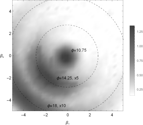
The linearization (46) breaks down when the absolute value of becomes large. We then perform a numerical integration of the full wave packet66 6 The wave packet is rescaled by the inverse of the van Vleck factor. . Fig. 5(a) shows the results for and different values of . For , the wave packet has a global maximum which corresponds to the analytical result (47). For increasing , the wave packet assumes an annular shape and propagates outwards with decreasing amplitude. The wave is peaked in the direction of negative . For decreasing , one has a similar behavior with the maximum moving into the opposite direction. Note that this annular waves also appear for the corresponding wave packet of the Kasner solution. The dispersion takes place due to the additional degrees of freedom introduced by the anisotropy.
In Fig. 5(b) we display the maxima of the wave packet for different together with a Gaussian fit to the peak region. One can see that close to the peak the wave packet decreases like a Gaussian, but decays much weaker (not even exponentially) further away. The amplitude of the full wave packet including the van Vleck determinant will increase for decreasing such that the peak along the classical trajectory will be at best a local maximum. This might be interpretable as a transition from a semiclassical into a full quantum regime.
The Klein-Gordon flux does not vanish. Similar to the case considered in the previous section, the exponential function from the van Vleck determinant cancels, yielding
| (48) | ||||
where , and means that both and are proportional to the expression on the right-hand side. Numerically we find for it a similar structure as for , that is, the Klein-Gordon flux is peaked over the classical trajectory. According to criterion 2, the big rip is not avoided. Similar to the case of the last section, the singularity is thus only avoided by the DeWitt criterion. This explicit calculation shows, moreover, that the wave packet is not peaked all along the classical trajectory if one considers , whereas it is peaked with respect to the Klein-Gordon flux.
VI Conclusion
In this paper, we have extended previous investigations of singularity avoidance from isotropic to anisotropic models. We have, in particular, adapted the avoidance criterion to the covariant structure of minisuperspace, which becomes relevant for dimensions higher than two. We have found that the DeWitt criterion can, in general, be fulfilled, but not so the vanishing of the Klein-Gordon current. For the reasons mentioned, however, we attribute more relevance to the DeWitt criterion.
The flux criterion was recently applied in DS19 to investigating the fate of (big bang and big crunch) singularities in FLRW models with Brown-Kuchař dust. Singularity avoidance was then found for a certain class of factor orderings.
In our paper, singularity avoidance was found by studying properties of the quantum cosmological Wheeler-DeWitt equation. The structure of this differential equation was used to disclose the fate of both the big bang and the big rip singularities. The tacit assumption in this is that information about the fates of different types of singularities can be obtained from one and the same differential equation (in the same way as information about different types of classical singularities can be obtained from the same Friedmann-Lemaître equations). A full mathematical treatment should address the properties of the Wheeler-DeWitt equation and its boundary conditions in much more detail, pointing out structural differences between the singularities, but this is beyond the scope of this paper.
While the general criteria were formulated for general Bianchi class A models, detailed investigations were made for the Bianchi I model with and without matter. Bianchi I models admit the prototype of an asymptotically velocity term dominated (AVTD) model. Our results of singularity avoidance should thus be representative for such a kind of singularity with a sufficiently large number of degrees of freedom. Other Bianchi models such as Bianchi VIII and Bianchi IX exhibit an oscillatory behavior when approaching the singularity. The singularity can, however, become AVTD if, for example, a scalar field is added Berger.
Because Bianchi IX models are generally considered as reflecting the generic behavior towards a spacelike singularity, future investigations of singularity avoidance should attempt to address these models in as much detail as possible. For this, it would be desirable to have mathematical theorems available such as those discussed here for the Kasner solution. In Ringstroem_Book one finds an existence and uniqueness theorem (Theorem 8.6 there), but for the Bianchi IX potential no decay rate estimates seem to exist. The Wheeler-DeWitt equation for the vacuum Bianchi IX (mixmaster) model was solved numerically in Koehn by using the ‘hard wall approximation’. The results found in this analysis strongly indicate the decay of wave packet amplitudes.
It is generally believed that the approach to a spacelike singularity at the level of the full Einstein equations can be described by the Belinsky-Khalatnikov-Lifshits (BKL) scenario; see, for example, Berger; KKP18 and references therein. This corresponds to a decoupling of spatial points, in which every spatial point exhibits the dynamics of a separate Bianchi IX model. The eventual goal will be to present a quantum-gravitational analysis of this situation, from which one should be able to draw general conclusions about singularity avoidance. An investigation in the framework of affine quantization was made recently in GPP19. Attempts in this direction using the Wheeler-DeWitt equation will be the subject of future investigations.
Acknowledgments
We are grateful to Anne Franzen and Tim Schmitz for helpful discussions.
References
- (1) C. Kiefer, Quantum Gravity. Third edition (Oxford University Press, Oxford, 2012).
- (2) G. Calcagni, Classical and Quantum Cosmology, Graduate Texts in Physics (Springer International Publishing Switzerland, 2017).
- (3) Springer Handbook of Spacetime, edited by A. Ashtekar and V. Petkov (Springer, Berlin, 2014).
- (4) M. Bojowald, Quantum Cosmology, Lecture Notes in Physics 835 (Springer, New York, 2011).
- (5) E. Wilson-Ewing, Class. Quantum Grav. 35, 065005 (2018).
- (6) B. S. DeWitt, Phys. Rev. 160, 1113 (1967).
- (7) J. A. Wheeler, in: Battelle rencontres, edited by C. M. DeWitt and J. A. Wheeler (Benjamin, New York, 1968), pp. 242–307.
- (8) P. Hájíček and C. Kiefer, Int. J. Mod. Phys. D 10, 775 (2001); C. Kiefer, arXiv:1512.08346 [gr-qc]; C. Kiefer and T. Schmitz, Phys. Rev. D 99,126010 (2019).
- (9) M. P. Da̧browski, C. Kiefer, and B. Sandhöfer, Phys. Rev. D 74, 044022 (2006).
- (10) M. Bouhmadi-López, C. Kiefer, and P. Martín-Moruno, arXiv:1904.01836 [gr-qc].
- (11) A. Y. Kamenshchik, Class. Quantum Grav. 30, 173001 (2013).
- (12) A. Kamenshchik, C. Kiefer, and N. Kwidzinski, Phys. Rev. D 93, 083519 (2016).
- (13) I. Albarran, M. Bouhmadi-López, F. Cabral, and P. Martín-Moruno, J. Cosmol. Astropart. Phys. 11 (2015) 044.
- (14) I. Albarran, M. Bouhmadi-López, C. Kiefer, J. Marto, and P. Vargas Moniz, Phys. Rev. D 94, 063536 (2016).
- (15) A. K. Sanyal and B. Modak, Phys. Rev. D 63, 064021 (2001); ibid., Class. Quantum Grav. 19, 515 (2002); A. Alonso-Serrano, M. Bouhmadi-López, and P. Martín-Moruno, Phys. Rev. D 98, 104004 (2018).
- (16) M. P. Ryan and L. C. Shepley, Homogeneous Relativistic Cosmologies (Princeton University Press, Princeton, 1975).
- (17) R. T. Jantzen, “Spatially homogeneous dynamics: a unified picture”, arXiv:gr-qc/0102035. Originally published in the Proceedings of the International School Enrico Fermi, Course LXXXVI (1982) on Gamov Cosmology, edited by R. Ruffini and F. Melchiorri (North Holland, Amsterdam, 1987), pp. 61–147.
- (18) C. Misner, in Magic without Magic: John Archibald Wheeler, edited by J. Klauder (Freeman, San Francisco, 1972), pp. 441–473.
- (19) B. S. DeWitt, in Relativity, edited by M. Carmeli, S. I. Fickler, and L. Witten (Plenum Press, New York, 1970), pp. 359–374.
- (20) J. J. Halliwell, Phys. Rev. D 38, 2468 (1988).
- (21) J. M. Lee and T. H. Parker, Bull. Am. Math. Soc. 17, 37 (1987).
- (22) A. Vilenkin, Phys. Rev. D 39, 1116 (1989).
- (23) A. O. Barvinsky, A. Yu. Kamenshchik, C. Kiefer, and C. F. Steinwachs, Phys. Rev. D 81, 043530 (2010).
- (24) S. W. Hawking and D. N. Page, Nucl. Phys. B 264, 185 (1986).
- (25) J. J. Halliwell, in: Quantum Cosmology and Baby Universes, edited by S. Coleman et al. (World Scientific, Singapore, 1991), pp. 159–243.
- (26) B. K. Berger, in: handbook, pp. 437–460.
- (27) C. Kiefer and H. D. Zeh, Phys. Rev. D 51, 4145 (1995).
- (28) T. Christodoulakis, T. Gakis, and G. O. Papadopoulos, Class. Quantum Grav. 19, 1013 (2002).
- (29) M. Bouhmadi-López, C. Kiefer, B. Sandhöfer, and P. V. Moniz, Phys. Rev. D 79, 124035 (2009).
- (30) M. Bouhmadi-López, C. Kiefer, and M. Krämer, Phys. Rev. D 89, 064016 (2014).
- (31) C. Kiefer, Phys. Rev. D 38, 1761 (1988).
- (32) V. Gorini, A. Y. Kamenshchik, U. Moschella, and V. Pasquier, Phys. Rev. D 69, 123512 (2004).
- (33) S. Klainerman, Comm. Pure Appl. Math. 38, 321 (1985).
- (34) T. Demaerel and W. Struyve, arXiv:1904.09244 [gr-qc].
- (35) H. Ringström, The Cauchy Problem in General Relativity, ESI Lectures in Mathematics and Physics, Volume 6 (ESI, 2009).
- (36) M. Köhn, Phys. Rev. D 85, 063501 (2012).
- (37) C. Kiefer, N. Kwidzinski, and W. Piechocki, Eur. Phys. J. C 78, 691 (2018).
- (38) A. Góźdź, W. Piechocki, and G. Plewa, Eur. Phys. J. C 79, 45 (2019).